A Novel Analytical Formulation of the Magnetic Field Generated by Halbach Permanent Magnet Arrays

Abstract

This paper presents an analytical study of the air-gap magnetic field of a surface permanent magnet (SPM) linear, slot-less machine with a Halbach PM configuration, under the no-load condition. While other analytical formulations of the magnetic field generated by PMs are available, they exhibit some drawbacks, such as only providing a Fourier series, or being suitable to determine magnetic field average values, but not local magnetic field distributions. On the contrary, the proposed approach allows the determination of a unique, closed-form formulation for the slot-less machine air-gap field. This is obtained starting from the complex expression of the magnetic field of a conductor, inside the air gap, between two parallel smooth iron surfaces, obtained by means of the method of images. The magnetic field due to an infinitesimal conductor belonging to a current sheet is then integrated along a segment, providing the expression of the magnetic field due to the corresponding linear current density distribution, for current sheets perpendicular or parallel to the iron surfaces. Any Halbach PM segment disposition can, hence, be obtained via a suitable combination of field distributions generated by couples of current sheets with perpendicular and parallel orientation. Lastly, the no-load magnetic field expression with a Halbach array of PMs is retrieved. The proposed analytical model provides an accurate representation of the magnetic field distribution produced by any Halbach array, with an arbitrary number of segments and orientations. Additionally, the results obtained from the proposed analytical expressions are compared with FEM simulations realized by commercial software, and show an excellent agreement.

1. Introduction

The Halbach configuration of surface permanent magnet (SPM) machines has been extensively studied in the last years, and widely used in several electrical machines, thanks to its relevant operating features, such as the good quality of the air-gap flux density distribution, and the limited impact of the armature reaction on the air-gap field. Compared to classical configurations, where the permanent magnets are magnetized in a normal direction with respect to the iron surfaces, the Halbach configuration exhibits several benefits, the most remarkable and important of which are: the presence of a higher flux density in the air gap, together with a mass reduction in the mover core [1], and the presence of a nearly sinusoidal air-gap flux density distribution, which generates an almost-sinusoidal back electromotive force (BEMF) with a low harmonic content. The reduction in the air-gap flux density harmonics drastically reduces the cogging torque, with no need to apply rotor or stator skewing [2].

However, the magnetization procedure of an ideal Halbach array is complex and expensive, which is clearly in contrast with the need to cut costs in electric motor serial production. Consequently, the use of this technology is limited to special applications, where performance cannot be degraded in favour of costs. In order to overcome these issues, the most common and cheap solution applied in industry is segmented magnetization, which consists of dividing the magnet into several segments, which are magnetized to reproduce a normal flux density component as close as possible to a sine wave [3,4,5]. However, a closed-form analytical model of the air-gap field resulting from this configuration is not available in the literature.

Indeed, several analytical methods have been developed to study the air-gap magnetic field distribution produced by permanent magnets, and some of them can also be applied to Halbach arrays.

The most popular analytical method is the subdomain method, which derives an overall model via solving several two-dimensional problems, each referring to different regions (slots, slot opening, air gap, rotor magnets, etc.). Subsequently, through a variable separation, the magnetic vector potential distribution is obtained as a Fourier series [6,7,8,9]. The method also works well with slot openings, and with machines with iron cores, although the obtained solution is not provided in closed form, but in a Fourier series.

The lumped parameter magnetic circuit method is sometimes used alternatively, and consists of dividing the magnetic flux paths inside the air gap into several branches [10,11,12,13]. Unfortunately, this method, although practical and simple to implement, is only suitable for calculating magnetic field average quantities, and not local magnetic field distributions.

More suitable models for the study of local magnetic field distributions are presented in [14,15], where an analytical closed-form solution is found, making use of the Ampère and Biot–Savart laws. However, these methods are valid only for non-magnetic core machines (no iron is present).

In order to overcome these limitations, in this paper, a novel closed-form analytical solution for the magnetic field generated by a permanent magnet with any magnetizing angle is retrieved. This is obtained through the use of the method of images, and through taking advantage of the duality principle between the electric and magnetic field. Then, the model of the air-gap field is obtained for any Halbach array of electrical machines equipped with iron cores. The proposed method is very easy to implement, and provides a quick field solution compared with FEM simulation, while maintaining a very high accuracy level.

The paper is organized as follows. In Section 2, the disposition of the Halbach array is described, together with the main properties of this configuration.

The analytical expression of the magnetic field distribution produced by a single PM segment is retrieved in Section 3. In particular, in Section 3.1, the initial assumptions of the method are introduced, together with its starting formulas. In Section 3.2 and Section 3.3, current sheets with normal and tangential disposition with respect to the iron surfaces are considered, and the corresponding field formulations are retrieved. Then, in Section 3.4 and Section 3.5, making use of two couples of parallel normal and tangential current sheets, the elementary blocks of surface permanent magnets, normally and tangentially magnetized, are obtained, and the generated field distributions are compared with FEM simulations. In Section 3.6, by combining the two permanent magnet elementary blocks, the formulation of a Halbach PM segment, magnetized according to an angle θ_pm, is retrieved, and is compared with FEM simulations.

In Section 4, the analytical expressions of the magnetic field distribution generated by two different Halbach arrays, composed of 6 and 10 identical-width segments, are built. The field distributions obtained by those two arrays were compared with FEM simulations, and an outstanding agreement was shown, validating the model. In conclusion, the total harmonic distortion (THD) and harmonic spectra of the normal flux density distribution are shown for a different number of PM segments.

Finally, in Section 5, the computational times of the analytical formulation and of the FEM simulations are compared, for the different configurations, in order to support the effectiveness of the proposed method in providing a fast, accurate evaluation of the magnetic field generated by Halbach arrays.

2. Halbach PM Disposition and Properties

The Halbach disposition of PMs, introduced in 1980 by Klaus Halbach [16], is very popular in several electromagnetic devices, such as motors [6], MagLev systems [17], eddy current brakes [18], actuators [19], magnetic bearings [20], and energy harvesting [21].

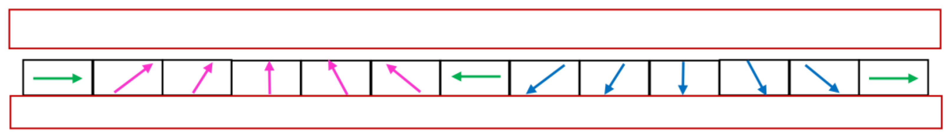
A Halbach array consists of a peripheral sequence of PM segments, with the progressive rotation of the magnetization orientation, as shown in the example of Figure 1.

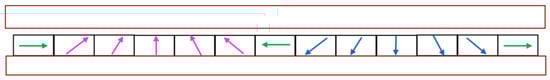
Figure 1. Example of Halbach PM disposition: each segment magnetization is orientated as rotated by a constant angle with respect to the previous one; the group of segments identified by magenta arrows forms a north pole, while the group of segments identified by blue arrows forms a south pole.

A degree of freedom in this array is the number of PM segments per pole (six in the example depicted in Figure 1, including, in each pole, the left segment with a horizontal magnetization orientation).

The main features of this disposition are:

-

the flux density distribution amplitude is reinforced in the upper surface of the array, in the air gap, while it is weakened in the lower surface;

-

this different distribution leads to the strengthening of the magnetic field where the tangential force is produced, while it reduces the need for a thick yoke width, lightening the mass and the inertia of the moving part;

-

through the increase in the number of segments per pole, the shape of the normal flux density distribution in the air gap becomes almost sinusoidal, which leads to the obtention of more sinusoidal EMF waveforms in the windings, and a smoother force with reduced ripple;

-

of course, the increase in the number of segments per pole implies increasing tolerance issues in the Halbach array assembly, and higher costs for the device: this requires to find a trade-off between the performance quality and system complexity.

3. Magnetic Field between Smooth Ferromagnetic Surfaces

In this section, the analytical model developed for the study of the no-load air-gap magnetic field between parallel, smooth, ideal ferromagnetic surfaces is introduced, and its initial assumptions and limitations are discussed.

3.1. Introduction to the Model and Elementary Blocks

In [22], the magnetic field distribution generated by a surface permanent magnet inside the air gap of a linear slotted machine has been investigated, and in [23], the air-gap field distribution has been obtained for the armature reaction, due to stator windings. Both the models were created via an analytical approach based on the method of images [24].

In the following, the aforementioned method, which has been proven to work very well for surface permanent magnets magnetized normally with respect to the iron surfaces, will be adapted in order to model the field produced by more complexly magnetized permanent magnet dispositions, such as the Halbach example.

The entire model lies on a complex analytical formulation of the magnetic field, and it makes use of the following assumptions and limitations:

• The stator and moving surfaces are supposed to be smooth, and separated by an air gap of uniform width;
• The magnetic field is solved in 2D, lying in the paper plane, and assumed invariant in the direction perpendicular to the paper plane;
• The machine is supposed to extend indefinitely in the direction perpendicular to the paper plane, so that the end effects are negligible;
• The relative recoil permeability (typically in the range 1.05–1.10 for rare earth PM materials) is assumed to be equal to the vacuum permeability (µ_r = 1); thus, at each point inside the air-gap width, it is assumed that B(z) = μ_o∙H(z) occurs, both in air and in the PMs;
• The iron permeability is assumed to be infinite, so the method of superimposition can be used;
• The iron parts are perfectly laminated; thus, no eddy current can be induced in the iron by the varying magnetic field;
• The conductors placed inside the air gap extend indefinitely perpendicular to the paper plane;
• The skin effect due to alternating currents flowing in the conductors is neglected.

It is well known in the literature that permanent magnets can be modeled using current sheets (the principle of equivalence, introduced by Ampère); the current densities of these current sheets are set equal to the magnet linearly extrapolated coercivity H_c0 [25,26]. The use of current sheets, suitably positioned in the space, allows us to model permanent magnets with different directions of magnetization. The problem is then usually solved according to the subdomain method, and the solution is retrieved in a Fourier series.

On the contrary, in the following, the magnetic field formulation of the current sheets that model the permanent magnet is retrieved analytically, giving a novel solution in closed form. The developed method starts from the complex formula [22]:

$${\mathit{H}}_c(z)=\frac{jI}{4g}\left[\coth \left(\frac{\pi }{2}\cdot \frac{\overline{z}-{\overline{z}}_p}{g}\right)+\coth \left(\frac{\pi }{2}\cdot \frac{\overline{z}-z_p}{g}\right)\right],$$

(1)

which describes the magnetic field produced via an indefinite wire powered by a current I, flowing outside the paper plane, and positioned between two smooth ideal iron surfaces, where z = x + jy is the complex coordinate of the point in which the field is calculated; z_p = x_p + jy_p is the complex coordinate where the current-carrying conductor is positioned; and z and z_p are the respective complex conjugates. With the use of this formula, the elementary blocks consisting of current sheets are built, in order to model different magnetization directions.

3.2. Air-Gap Magnetization Due to a Current Sheet Disposed Normally to the Iron Surfaces

The first disposition of the current sheet to be analyzed is shown in Figure 2.

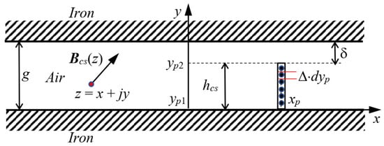
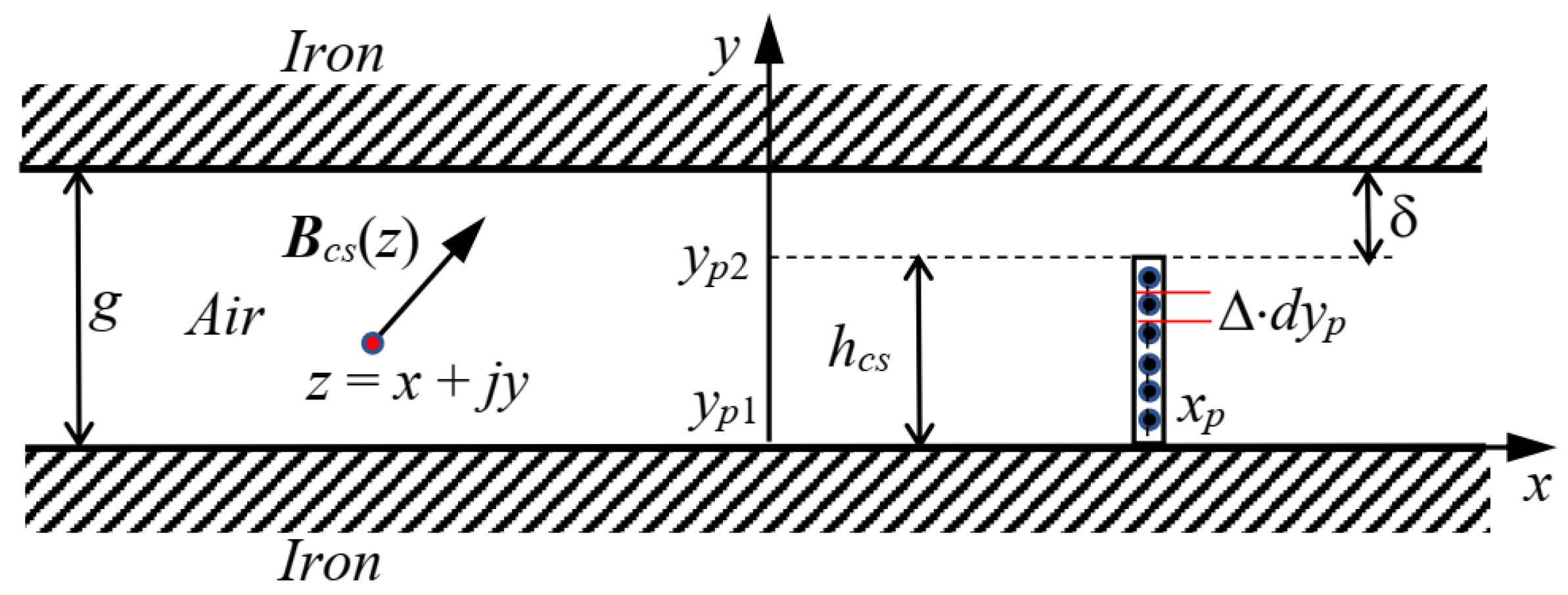
Figure 2. Graphical representation of the magnetic field H_ncs(z) evaluated at a point of coordinates z = x + jy in an air gap between two smooth, parallel iron surfaces, generated by a current sheet, normally orientated with respect to the iron surfaces, distributed along the points p, with coordinates z_p = x_p + jy_p.

Figure 2 shows a single vertical current sheet, normal to the iron surfaces, distributed along the points p, with coordinates z_p = x_p + jy_p, inside an air gap between two smooth ferromagnetic surfaces. The current sheet is powered by a current density ∆, equal to the magnet linearly extrapolated coercive force H_c0, flowing outside the paper plane.

If we consider an infinitesimal current sheet element ∆ × dy_p, according to (1), the infinitesimal magnetic strength air-gap complex vector at the point z can be written as:

$$d{\mathit{H}}_{cs}(z)=j\frac{\Delta \cdot d{y}_p}{4g}\left[\coth \left(\frac{\pi }{2}\cdot \frac{\overline{z}-x_p+j{y}_p}{g}\right)+\coth \left(\frac{\pi }{2}\cdot \frac{\overline{z}-x_p-j{y}_p}{g}\right)\right].$$

(2)

Integrating (2) between y_p1 = 0 and y_p2 = h_cs, the expression of the magnetic strength H_ncs(z) distribution, due to a current sheet orientated normally to the iron surfaces, is retrieved:

$${\mathit{H}}_{ncs}(z)=\frac{\Delta }{2\pi }\ln \left[\sinh \left(\frac{\pi }{2}\cdot \frac{\overline{z}-x_p+j{h}_{cs}}{g}\right)/\sinh \left(\frac{\pi }{2}\cdot \frac{\overline{z}-x_p-j{h}_{cs}}{g}\right)\right].$$

(3)

3.3. Air-Gap Magnetization Due to a Current Sheet Disposed Tangentially to the Iron Surfaces

The second current sheet disposition to be analyzed is depicted in Figure 3: it shows a single horizontal current sheet, tangential to the iron surfaces, distributed along the points p, with coordinates z_p = x_p + jy_p, inside an air gap between two smooth ferromagnetic surfaces. The current sheet is powered by a current density ∆ = H_c0 flowing outside the paper plane. If we consider an infinitesimal current sheet element ∆ × dx_p, according to (1), the infinitesimal-magnetic-strength air-gap complex vector in the point z can be written as:

$$d{\mathit{H}}_{cs}(z)=j\frac{\Delta \cdot d{x}_p}{4g}\left[\coth \left(\frac{\pi }{2}\cdot \frac{\overline{z}-x_p+j{y}_p}{g}\right)+\coth \left(\frac{\pi }{2}\cdot \frac{\overline{z}-x_p-j{y}_p}{g}\right)\right].$$

(4)

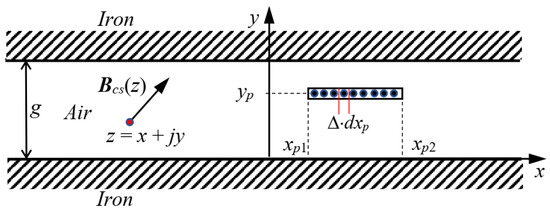
Figure 3. Graphical representation of the magnetic field H_tcs(z) evaluated at a point of coordinates z = x + jy in an air gap between two smooth, parallel iron surfaces, generated by a current sheet, tangentially orientated with respect to the iron surfaces, distributed along the points p, with coordinates z_p = x_p + jy.

Through integrating (4) between x_p1 and x_p2, the expression of the magnetic strength distribution H_tcs(z), due to a current sheet orientated tangentially to the iron surfaces, is retrieved:

$${\mathit{H}}_{tcs}(z)=j\frac{\Delta }{2\pi }\left\{\ln \left[\frac{\sinh \left(\frac{\pi }{2}\cdot \frac{\overline{z}-x_{p1}+j{y}_p}{g}\right)}{\sinh \left(\frac{\pi }{2}\cdot \frac{\overline{z}-x_{p2}+j{y}_p}{g}\right)}\right]+\ln \left[\frac{\sinh \left(\frac{\pi }{2}\cdot \frac{\overline{z}-x_{p1}-j{y}_p}{g}\right)}{\sinh \left(\frac{\pi }{2}\cdot \frac{\overline{z}-x_{p2}-j{y}_p}{g}\right)}\right]\right\}.$$

(5)

Through using (3) and (5), both normally and tangentially magnetized PMs can be modelled.

3.4. PM Magnetized along an Axis Orientated Normally to the Iron Surfaces

The first PM we want to model is a magnet magnetized normally with respect to the iron surfaces, orientated along the y axis, as shown in Figure 4.

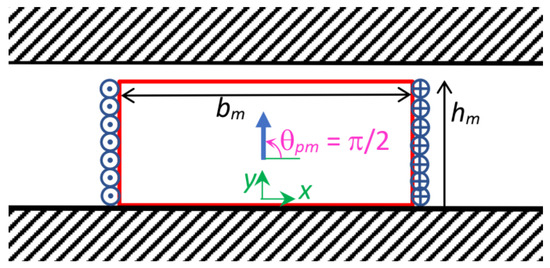
Figure 4. Permanent magnet with h_m height and b_m width, centred with respect to the origin, with magnetization orientated normally to the iron surfaces along the y axis (north PM, magnetization angle θ_pm = π/2 with respect to the x axis), modelled with two current sheets positioned, respectively, in x_p = +b_m/2 and x_p = −b_m/2, with a linear current density, respectively, equal to (−Δ) and (+Δ).

A PM with h_m height and b_m width, centered with respect to the origin, and magnetized normally with respect to the iron surfaces, along the y axis (north PM), is modelled with two current sheets: one positioned in x_p = +b_m/2, and with a negative linear current density (−Δ); the other one positioned in x_p = −b_m/2, and with a positive linear current density (+Δ). For both the current sheets, it holds that y_p2 = h_cs = h_m; thus, via (3), the magnetic strength distribution H_PM.n(z), due to a centered PM, magnetized normally to the iron surfaces, can be expressed as follows:

$${\mathit{H}}_{PM.n}(z)=\frac{\Delta }{2\pi }\left\{\ln \left[\frac{\sinh \left(\frac{\pi }{2}\cdot \frac{\overline{z}-b_m/2-j{h}_m}{g}\right)}{\sinh \left(\frac{\pi }{2}\cdot \frac{\overline{z}-b_m/2+j{h}_m}{g}\right)}\right]+\ln \left[\frac{\sinh \left(\frac{\pi }{2}\cdot \frac{\overline{z}+b_m/2+j{h}_m}{g}\right)}{\sinh \left(\frac{\pi }{2}\cdot \frac{\overline{z}+b_m/2-j{h}_m}{g}\right)}\right]\right\}.$$

(6)

In the case that the PM is south magnetized, it is enough to put a minus sign before the second member of (6).

Moreover, if the PM magnetized normally to the iron surfaces is displaced by Δx to the right of the origin, the corresponding magnetic strength follows from (6), via the following translation:

H_{PM.n_Δx}(z) = H_PM.n(z − Δx).

(7)

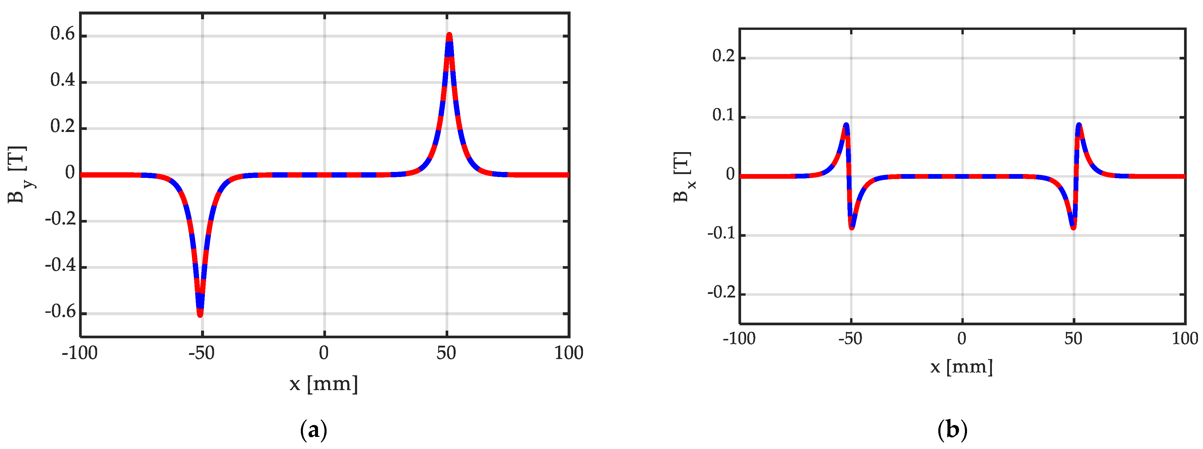
Figure 5 shows the distribution of the y and x components of B_PM.n = μ_o∙H_PM.n, corresponding to B_y = Im(B_PM.n) and to B_x = Re(B_PM.n), respectively, due to a single normally magnetized PM, obtained via the proposed closed-form, analytical expression (6), compared with a FEM 2D simulation realized with a commercial software [27], used as a benchmark, for b_m = 102 mm, h_m = 10 mm, g = h_m + δ = 11.5 mm. As can be observed, the agreement is excellent, with the curves obtained by means of the proposed closed-form analytical expressions being perfectly superimposed with the benchmark obtained from the commercial FEM solver.

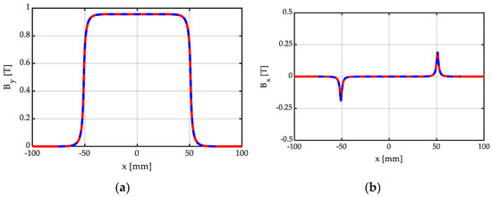
Figure 5. Distribution of the (a) y and (b) x components of B_PM.n = μ_o∙H_PM.n, due to a single normally magnetized PM, obtained analytically (continuous red line) via (6), and via a FEM 2D simulation (dashed blue line), for b_m = 102 mm, h_m = 10 mm, g = h_m + δ = 11.5 mm.

3.5. PM Magnetized along an Axis Tangentially Orientated to the Iron Surfaces

In this subsection, we consider a PM tangentially magnetized, as shown in Figure 6. A PM with h_m height and b_m width, centered with respect to the origin, and tangentially magnetized, in a horizontal direction along the x axis (north PM toward the right), is modelled with two current sheets: one positioned in y_p = 0, and with a negative linear current density (−Δ); the other one positioned in y_p = h_m, and with a positive linear current density (+Δ). Both the current sheets are centered at the origin, with x_p1 = −b_m/2; x_p2 = +b_m/2.

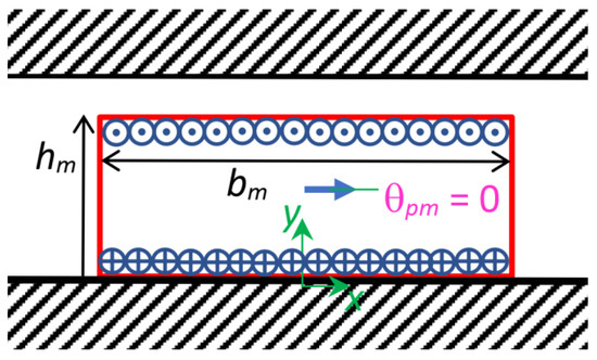
Figure 6. Permanent magnet with h_m height and b_m width, centered at the origin, with magnetization orientated tangentially with respect to the iron surfaces along the x axis (north PM, magnetization angle θ_pm = 0 with respect to the x axis), modelled with two current sheets positioned, respectively, in y_p = 0 and y_p = h_m, with a linear current density, respectively, equal to (−Δ) and (+Δ).

Thus, via (5), the magnetic strength distribution between the two smooth ferromagnetic surfaces, due to a centered, tangentially right-magnetized PM, H_PM.t(z), is expressed as:

$$\begin{array}{l}{\mathit{H}}_{PM.t}(z)=j\frac{\Delta }{2\pi }\cdot \left\{\ln \left[\frac{\sinh \left(\frac{\pi }{2}\cdot \frac{\overline{z}+b_m/2+j{h}_m}{g}\right)}{\sinh \left(\frac{\pi }{2}\cdot \frac{\overline{z}-b_m/2+j{h}_m}{g}\right)}\right]+\ln \left[\frac{\sinh \left(\frac{\pi }{2}\cdot \frac{\overline{z}+b_m/2-j{h}_m}{g}\right)}{\sinh \left(\frac{\pi }{2}\cdot \frac{\overline{z}-b_m/2-j{h}_m}{g}\right)}\right]+\right.\\ \left.-2\cdot \ln \left[\frac{\sinh \left(\frac{\pi }{2}\cdot \frac{\overline{z}+b_m/2}{g}\right)}{\sinh \left(\frac{\pi }{2}\cdot \frac{\overline{z}-b_m/2}{g}\right)}\right]\right\}\end{array}.$$

(8)

Additionally, for this kind of magnetization, if the PM is displaced by Δx to the right of the origin, the corresponding magnetic strength follows from (8) via the following translation:

H_{PM.t_Δx}(z) = H_PM.t(z − Δx).

(9)

Figure 7 shows the distribution of the y and x components of B_PM.t = μ_o∙H_PM.t, corresponding to B_y = Im(B_PM.t) and to B_x = Re(B_PM.t), respectively, due to a single tangentially magnetized PM, obtained via the proposed closed-form, analytical expression (8), compared with a FEM 2D simulation realized with commercial software [27], used as a benchmark, for b_m = 102 mm, h_m = 10 mm, g = h_m + δ = 11.5 mm. In this case, also, the agreement is excellent, with the curves obtained by means of the proposed closed-form analytical expressions being perfectly superimposed with the benchmark obtained from the commercial FEM solver.

Figure 7. Distribution of the (a) y and (b) x components of B_PM.t = μ_o∙H_PM.y, due to a single tangentially magnetized PM, obtained analytically (continuous red line) via (8), and via an FEM 2D simulation (dashed blue line), for b_m = 102 mm, h_m = 10 mm, g = h_m + δ = 11.5 mm.

3.6. Halbach PM Segment with Magnetization Orientated according to an Angle θ_pm

As known, if the magnetization vector $\overrightarrow{M}$ of a PM is that of a generic Halbach segment, orientated according to an angle θ_pm with respect to the x axis, it can be decomposed in the form:

$$\overrightarrow{\mathit{M}}=M_x\cdot \widehat{x}+M_y\cdot \widehat{y},$$

(10)

where $\widehat{x}$ and $\widehat{y}$ are versors of the x and y axis, respectively.

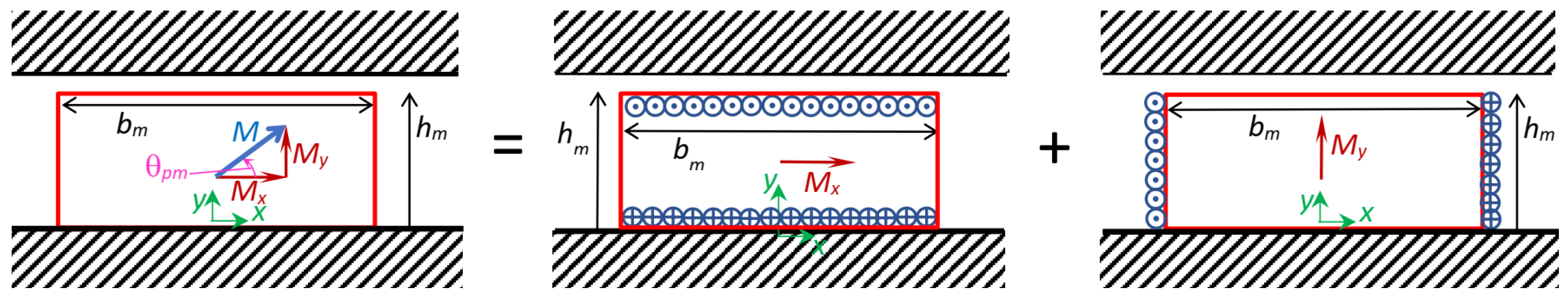
This situation can be represented as shown in Figure 8, where the superposition of the x and y magnetization vectors is applied, and the corresponding current sheet couples are shown. The amplitudes of the two magnetization vector components are expressed as:

$$M_x=M\cdot \cos \left({\theta }_{pm}\right),M_y=M\cdot \sin \left({\theta }_{pm}\right).$$

(11)

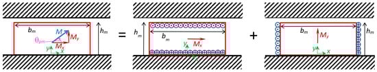
Figure 8. A Halbach permanent magnet segment with h_m height and b_m width and magnetization vector $\overrightarrow{M}$, orientated according to the angle θ_pm with respect to the x axis, decomposed in the two PM with magnetization orientated according to the x and y vector components, respectively. The PM magnet orientated according to the x axis is modelled by means of two current sheets positioned, respectively, in y_p = 0 and y_p = h_m, with a linear current density, respectively, equal to (−Δ) and (+Δ), while the PM magnet, orientated according to the y axis, is modelled by means of two current sheets positioned, respectively, in x_p = +b_m/2 and x_p = −b_m/2, with a linear current density, respectively, equal to (−Δ) and (+Δ).

Based on (11), considering (6) and (8), the following resultant magnetic strength expression can be written at any point z between the two iron smooth surfaces, for a Halbach PM segment centered at the origin, with the orientation θ_pm:

$${\mathit{H}}_{H1}(z,{\theta }_{pm})={\mathit{H}}_{PM.t}(z)\cdot \cos \left({\theta }_{pm}\right)+{\mathit{H}}_{PM.n}(z)\cdot \sin \left({\theta }_{pm}\right).$$

(12)

Of course, via (7) and (9), the following translation equation can be applied to (12):

H_{H1_Δx}(z,θ_pm) = H_H1(z − Δx, θ_pm).

(13)

Figure 9 shows the distribution of the y and x components of B_H.1 = μ_o∙H_H.1, corresponding to B_y = Im(B_H.1) and to B_x = Re(B_H.1), respectively, due to a single magnetized PM with orientation θ_pm = 30°, obtained via the proposed closed-form, analytical expression (12), compared with a FEM 2D simulation realized with commercial software [27], used as a benchmark, for b_m = 102 mm, h_m = 10 mm, g = h_m + δ = 11.5 mm. In this case, also, the agreement is excellent, with the curves obtained by means of the proposed closed-form analytical expressions being perfectly superimposed with the benchmark obtained from the commercial FEM solver.

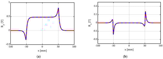
Figure 9. Distribution of the (a) y and (b) x components of B_H.1 = μ_o∙H_H.1, due to a single PM magnetized with orientation θ_pm = 30°, obtained analytically (continuous red line) via (12) and via a FEM 2D simulation (dashed blue line), for b_m = 102 mm, h_m = 10 mm, g = h_m + δ = 11.5 mm.

4. The Halbach PM Arrays

Halbach Array Using the PM Segment Model

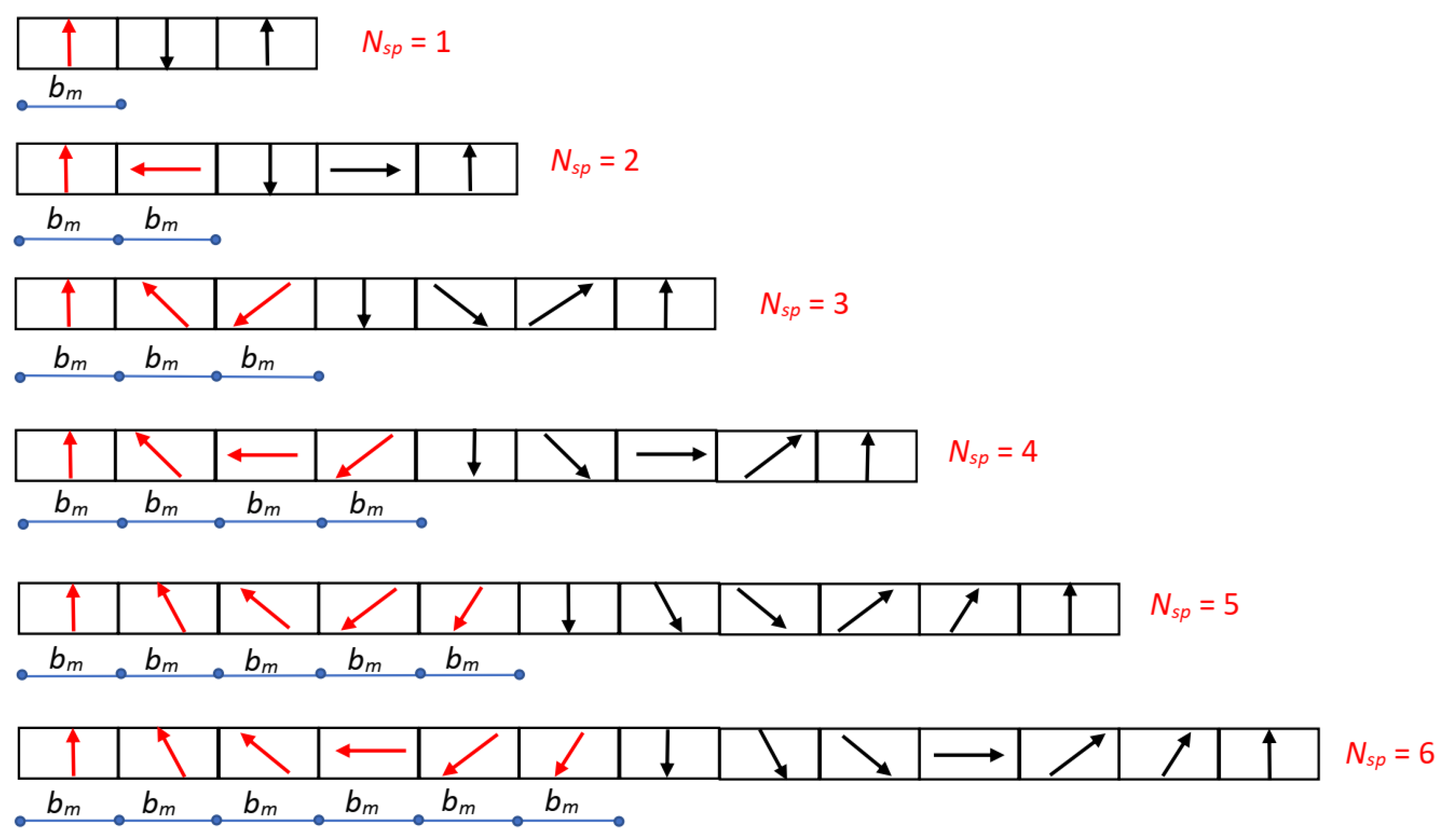
In this paper, we limit our analysis to Halbach PM arrays consisting of PM segments, all with the same peripheral width b_m. Figure 10 shows some examples of this type of Halbach array. The PM segments belonging to the same pole are shown with magnetization vectors drawn in red, and the change in the orientation angle between adjacent segments is the same. The number of PM segments per pole is indicated with N_sp: Figure 10 shows some Halbach array dispositions, from N_sp = 1 (which is a degenerate case) to N_sp = 6.

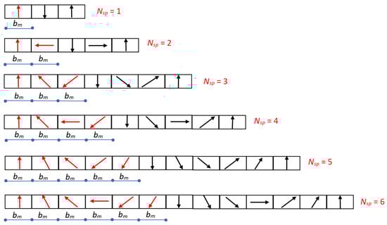
Figure 10. Halbach permanent magnet arrays with N_sp segments/pole ranging from 1 to 6, and magnetization vectors highlighted in red; all segments have the same peripheral width b_m = τ/N_sp and the same angular displacement between adjacent magnetization vectors, equal to β_m = π/N_sp [rad].

Let us define the pole pitch τ as the peripheral extension of one pole, measured along the air gap. Based on the hypothesis of uniform segment peripheral extension, the following equation holds:

$$b_m=\tau /N_{sp}.$$

(14)

Moreover, considering that the angular extension of one pole equals π electrical radians, the angular displacement β_m between adjacent magnetization vectors, equal all along the periphery, is given by:

$${\beta }_m=\pi /N_{sp}.$$

(15)

The angle of the magnetization vector of the j_m-th PM segment (j_m = 1, 2,…, N_sp) equals:

$${\theta }_{p{m}_{jm}}=\pi /2+(j_m-1)\times {\beta }_m$$

(16)

From (12), for a PM segment centered at the origin, acting alone, the flux density distribution in the air gap is expressed as:

$${\mathit{B}}_{H1}(z,{\theta }_{pm})={\mathit{B}}_{PM.t}(z)\cdot \cos \left({\theta }_{pm}\right)+{\mathit{B}}_{PM.n}(z)\cdot \sin \left({\theta }_{pm}\right).$$

(17)

and via (13), the j_m-th segment, acting alone, produces the following flux density:

$${\mathit{B}}_H\left(z,j_m\right){=\mathit{B}}_{H1}\left[z-\left(j_m-1\right)\cdot b_m,{\theta }_{pm}{}_{j_m}\right].$$

(18)

Thus, the group of N_sp PM Halbach segments of one pole produces the following flux density distribution in the air gap:

$${\mathit{B}}_{H.1pole}\left(z\right)={\displaystyle \sum _{j_m=1}^{N_{sp}}{\mathit{B}}_H\left(z,j_m\right)}={\displaystyle \sum _{j_m=1}^{N_{sp}}{\mathit{B}}_{H1}\left[z-\left(j_m-1\right)\cdot b_m,{\theta }_{pm}{}_{j_m}\right]}.$$

(19)

However, in order to obtain a correct periodic distribution of flux density in the air gap, (19) must be extended on the left and on the right of the initial pole, by adding further distributions similar to (19) and displaced by integer multiples of the pole pitch τ.

If the extension is operated p times, both on the left and on the right, the multi-pole flux density distribution results in:

$${\mathit{B}}_{H.multi-pole}\left(z\right){=\mathit{B}}_{H.1pole}\left(z\right)+{\displaystyle \sum _{k=1}^p{\left(-1\right)}^k\cdot }{\mathit{B}}_{H.1pole}\left(z-k\cdot \tau \right)+{\displaystyle \sum _{k=1}^p{\left(-1\right)}^k\cdot }{\mathit{B}}_{H.1pole}\left(z+k\cdot \tau \right).$$

(20)

In (20), the factor (−1)^k equals 1 for even k values and −1 for odd k values, corresponding to the north and south pole groups of Halbach segments, respectively.

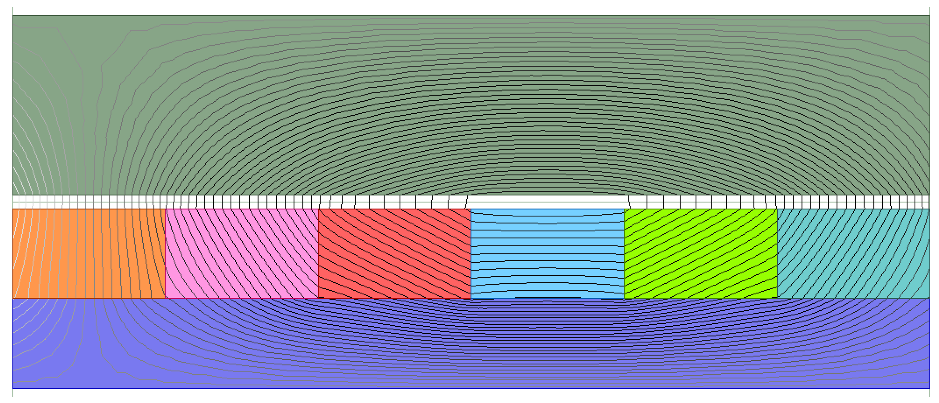
Figure 11 shows the field map of a Halbach array with N_sp = 6, calculated via a FEM 2D magnetostatic simulation realized with commercial software [27], used as a benchmark. In order to ensure the condition of periodicity, the adopted boundary conditions at the left and right ends are master–slave.

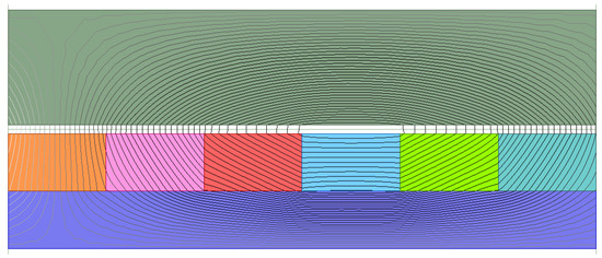
Figure 11. Field map of a Halbach array with N_sp = 6 segments/pole, each with the same width b_m, calculated via FEM 2D magnetostatic simulation realized with commercial software (numerical periodic solution based on master–slave boundary conditions): b_m = 17 mm; h_m = 10 mm; g = h_m + δ = 11.5 mm.

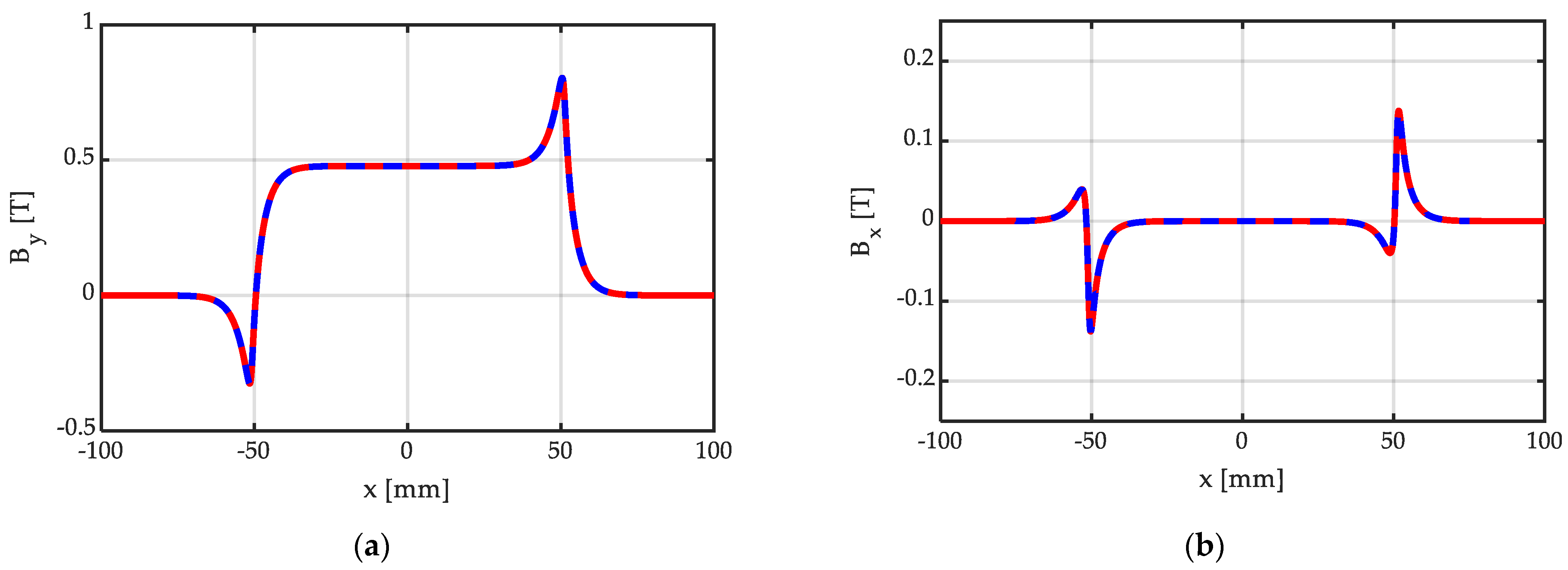
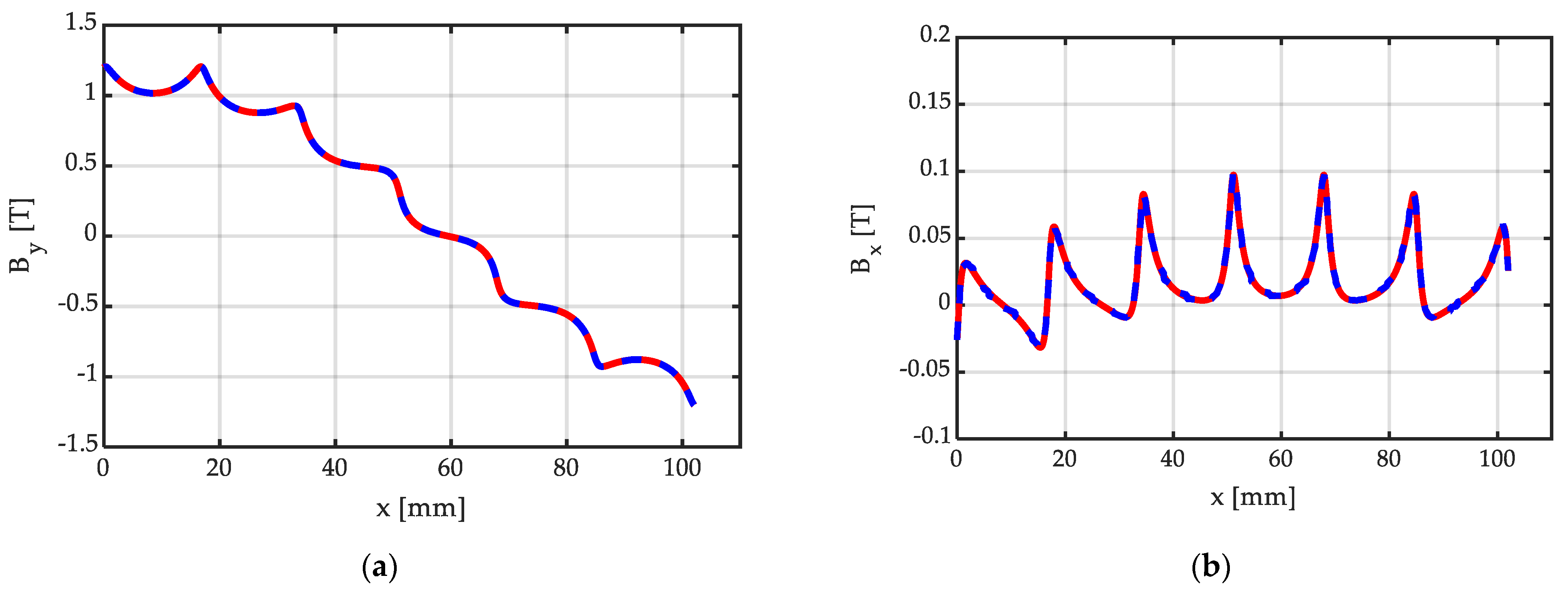
Figure 12 shows the corresponding y and x components of the flux density distribution along a line in the middle of the air gap, calculated via the proposed closed-form, analytical expression (20), and by FEM 2D simulation realized with commercial software [27], used as a benchmark. It can be observed that the agreement is excellent, with the curves obtained by means of the proposed closed-form analytical expressions being perfectly superimposed with the benchmark obtained from the commercial FEM solver. Additionally, as expected, B_y exhibits a roughly sinusoidal shape, while B_x is limited in amplitude, with a peak value in the order of 10% of the B_y peak value.

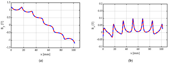
Figure 12. Distribution of the (a) y and (b) x components of B_H = μ_o∙H_H, due to the Halbach array of Figure 11, with N_sp = 6 PM segments/pole, all with width b_m = τ/N_sp: analytically calculated distribution (continuous red line) obtained via (20); numerically calculated distribution (dashed blue line), based on FEM 2D simulation with master–slave boundary conditions at the left and right ends, b_m = 17 mm, h_m = 10 mm, g = h_m + δ = 11.5 mm. The distributions have been calculated along the line at one-half the air-gap width, as drawn in Figure 11.

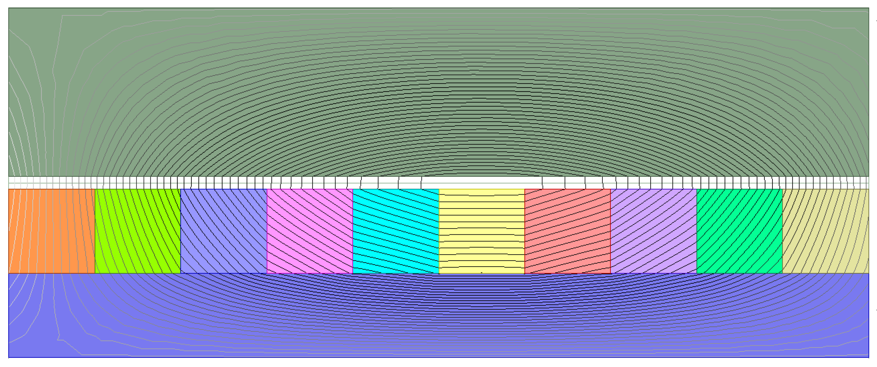
Figure 13 shows the field map of a Halbach array with N_sp = 10 segments/pole, each with the same width, calculated via FEM 2D magnetostatic simulation realized with commercial software [27], used as a benchmark. In this case, also, in order to ensure the condition of periodicity, the boundary conditions at the left and right ends are master–slave.

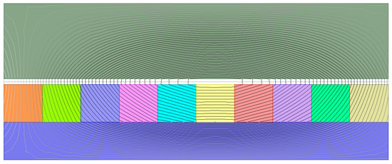
Figure 13. Field map of a Halbach array with N_sp = 10 segments/pole, each with the same width b_m, calculated via FEM 2D magnetostatic simulation realized with commercial software (numerical periodic solution based on master–slave boundary conditions): b_m = 10.2 mm; h_m = 10 mm; g = h_m + δ = 11.5 mm.

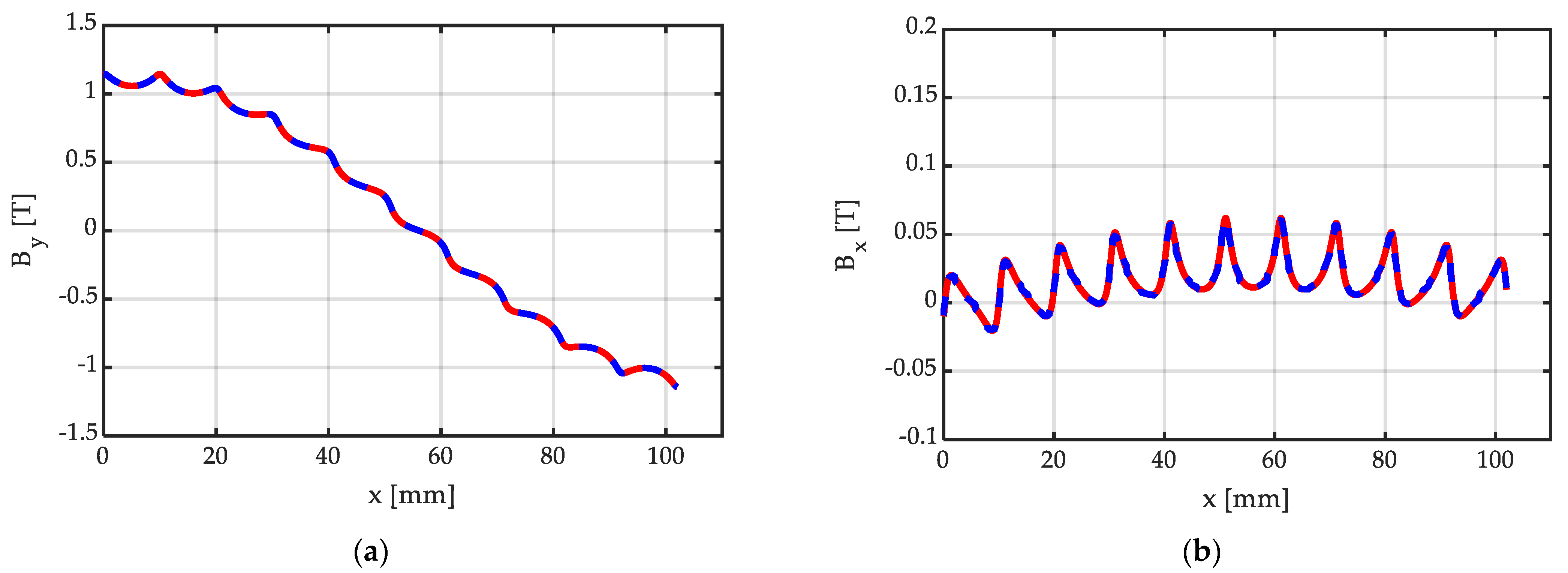
Figure 14 shows the corresponding y and x components of the flux density distribution along a line in the middle of the air gap, calculated via the proposed closed-form, analytical expression (20), and via FEM 2D simulation realized with commercial software [27], used as a benchmark. As can be observed, the agreement is excellent, with the curves obtained by means of the proposed closed-form analytical expressions being perfectly superimposed with the benchmark obtained from the commercial FEM solver. Additionally, as expected, the increase in N_sp implies a flux density distribution improvement, with an almost-sinusoidal shape of B_y, and a greatly reduced amplitude of the component B_x, with a peak value in the order of 5% of the B_y peak value.

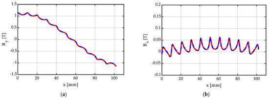
Figure 14. Distribution of the (a) y and (b) x components of B_H = μ_o∙H_H, due to the Halbach array of Figure 13, with N_sp = 10 PM segments/pole, all with width b_m = τ/N_sp: analytically calculated distribution (continuous red line) obtained via (20); numerically calculated distribution (dashed blue line), based on FEM 2D simulation with master–slave boundary conditions, b_m = 17 mm, h_m = 10 mm, g = h_m + δ = 11.5 mm. The distributions have been calculated along the line at one-half the air-gap width, as drawn in Figure 13.

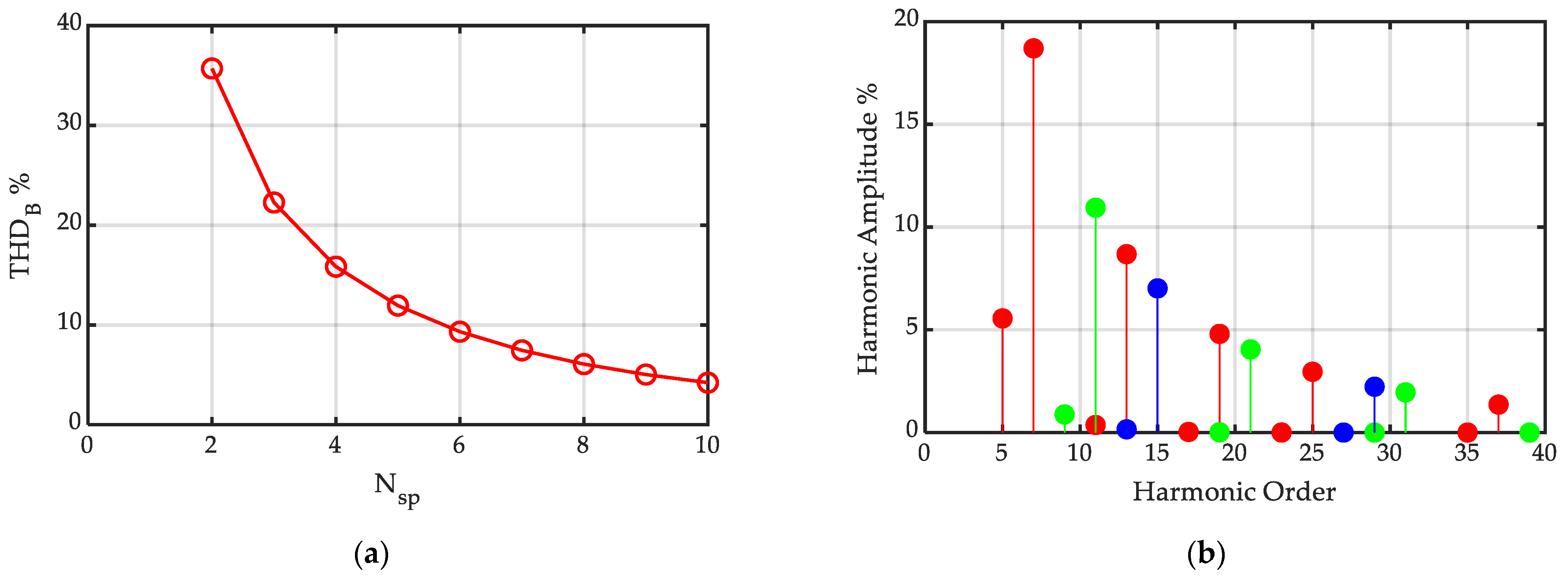
Finally, Figure 15 shows the harmonic content of the B_y flux density distribution, evaluated on the basis of the proposed closed-form, analytical expression (20) for Halbach arrays with different numbers of segments/pole.

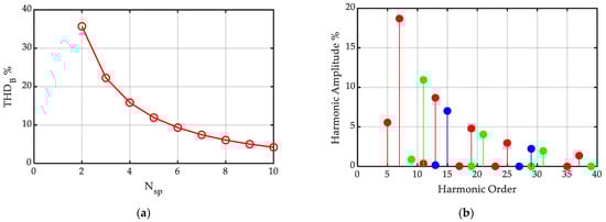
Figure 15. Harmonic content of the y component of the flux density distribution in the air gap of a Halbach PM array: (a) THD as a function of the number N_sp of segments/pole; (b) harmonic spectra of the y component of the flux density distribution in the air gap of a Halbach PM array for a number of segments/pole N_sp = 3 (red), N_sp = 5 (green), N_sp = 7 (blue), with τ = N_sp∙ b_m = 102 mm, h_m = 10 mm, g = h_m + δ = 11.5 mm.

In particular, Figure 15a reports the total harmonic distortion of the B_y flux density distribution as a function of the number of segments/pole N_sp in the Halbach array. As expected, the THD decreases with the increase in N_sp. Figure 14b reports the harmonic spectra of the B_y flux density distribution, evaluated on the basis of the proposed closed-form, analytical expression (20), expressed in a percentage with respect to the fundamental, and limited to a harmonic order equal to 40, for the cases of N_sp = 3 (red), N_sp = 5 (green), and N_sp = 7 (blue).

It is worth noting that, for any number of segments per pole N_sp, harmonics are present only in correspondence of harmonic orders satisfying the condition:

$$h=2k{N}_{sp}\pm 1,$$

(21)

where h is the harmonic order, and k ∈ ℕ.

5. Calculation Time Comparison between Analytical and FEM Approaches

In order to support the effectiveness of the proposed method in providing a fast, accurate evaluation of the magnetic field generated by Halbach arrays, the computational times of a number of PM arrangements, previously analyzed, are evaluated, for analytical and FEM field solutions. The same PC was used for both the analytical and FEM calculations, the features of which are detailed in Table 1, along with the software used. For the sake of conciseness, five example configurations have been considered, which are summarized in Table 2.

Table 1. Features of the PC and software used.

Intel Pentium Processor, CPU N4200, 1.10 GHz, 4 GB RAM
PC Operating System: Windows 10, 64 Bit
FEM software commercial tool:	Ansys Electronics Desktop 2021 R2
Software for the analytical calculation:	PTC MathCad 15.0

Table 2. Cases for the comparative analysis of the calculation times of the analytical and FEM approaches.

Case N°	Description
1	Single permanent magnet, centred with respect to the origin, with magnetization orientated normally to the iron surfaces (as depicted in Figure 4 and Figure 5)
2	Single permanent magnet centered in the origin, with tangential magnetization with respect to the iron surfaces (as depicted in Figure 6 and Figure 7)
3	Single Halbach permanent magnet segment with magnetization vector $\overrightarrow{M}$ orientated according to an angle θpm = 30° with respect to the x axis (as depicted in Figure 8 and Figure 9)
4	Halbach array with Nsp = 6 segments/pole, with the same peripheral width bm (as depicted in Figure 11 and Figure 12); two Halbach arrays at the left and at the right of the central array, for a total of five Halbach arrays
5	Halbach array with Nsp = 10 segments/pole, with the same peripheral width bm (as depicted in Figure 13 and Figure 14); two Halbach arrays at the left and at the right of the central array, for a total of five Halbach arrays

The comparison between the FEM and analytical simulations is reported in Table 3.

Table 3. Analytical and FEM approach calculation data. Number of calculation sampling points within one pole pitch: 500.

Case N°	Analytical Calculation	FEM Calculation				Δt Ratio
	Data	Data
	Calculation Time ΔtA [s]	Iterations N°	Energy Error [%]	Mesh Triangles N°	Computational Time ΔtF [s]	Comp. Times Ratio ΔtA/ΔtF [%]
1	0.12	8	3.21 × 10−4	4.99 × 104	20	0.58
2	0.07	14	1.34 × 10−4	2.40 × 105	67	0.10
3	0.08	13	1.36 × 10−4	1.86 × 105	66	0.13
4	0.20	12	3.08 × 10−4	4.95 × 104	18	1.11
5	0.27	12	3.77 × 10−4	4.80 × 104	16	1.68

For a correct interpretation of the presented results, it is worth considering that:

-

the number of calculated points adopted in the analytical method (500), uniformly distributed within the pole pitch τ, is chosen in a such a way to correctly reproduce the flux density distribution everywhere within τ, for all the considered cases of Table 2;

-

the calculation time in the analytical method corresponds to the total time needed to evaluate the x and y flux density components in the chosen number of points;

-

the calculation time in the FEM numerical approach corresponds to just the time to solve the field; it does not include the time needed to calculate the x and y flux density components in the chosen number of points.

Additionally, with respect to the accuracy of the results:

-

the accuracy of FEM analysis depends on the mesh refinement level, while the analytical field calculation in each point is direct, without any discretization refinement;

-

the calculation times of the cases 1, 2, and 3 are low (of the order of 0.1 s), while the calculation times of the cases 4 and 5 are higher (of the order of 0.2–0.3 s): in fact, the cases 1 and 2 include 2 current sheets, the case 3 includes 4 current sheets, while the case 4 includes 6 × (1 + 2 × 2) = 30 current sheets; finally, the case 5 includes 10 × (1 + 2 × 2) = 50 current sheets. In fact, generally, the field superposition of an higher number of current sheets requires an higher calculation time.

Overall, it is worth highlighting that, in all the considered configurations, the analytical calculation time is significantly lower than the time required in the numerical FEM approach, lower or around 1% of the corresponding FEM computational time. This is particularly significant in electrical machine design optimization, which requires repetitive simulations of possible design variations.

6. Conclusions

In this paper, an analytical method to study the flux density distribution generated into the air gap of a Halbach SPM slot-less machine under no-load conditions is proposed. Starting from the model of a single conductor between two smooth iron surfaces, the analytical formulations of current sheets, orientated both normally and tangentially to the faced ferromagnetic surfaces, is developed. Thus, by considering two parallel current sheets, both PMs magnetized normally and PMs magnetized tangentially to the ferro-magnetic surfaces are modelled. Through adding the field solutions for normal and tangential PMs, multiplied by the sinus and cosinus of the magnetization angle with respect to the x axis, the Halbach PM segment with any magnetization orientation can be modelled, and the model of a Halbach array with any number of segments per pole is obtained. The presented analytical model exhibits an excellent agreement with magneto-static FEM simulations, both in terms of air-gap field distribution waveforms, and in terms of harmonic spectra. However, the required calculation time is significantly lower. The ease and rapidity exhibited by the model makes it perfectly suitable for carrying out machine optimization, especially during the pre-design phase.

By using appropriately suited slotting functions [1,2], the present method can be extended to evaluate the field in the air gap of a slotted machine, with a fair accuracy level.

Future works will address the use of conformal mapping, to extend the present method to different geometries, such as cylindrical machines. Moreover, an extension of the proposed method to saturated conditions (saturable ferromagnetic material) is under development.

References

- Koo, M.-M.; Choi, J.-Y.; Shin, H.-J.; Kim, J.-M. No-Load Analysis of PMLSM With Halbach Array and PM Overhang Based on Three-Dimensional Analytical Method. IEEE Trans. Appl. Supercond. 2016, 26, 0604905. [Google Scholar] [CrossRef]
- Zhu, Z.Q.; Howe, D. Halbach permanent magnet machines and applications—A review. Proc. Inst. Elect. Eng. Electr. Power Appl. 2001, 148, 299–308. [Google Scholar] [CrossRef]
- Okita, T.; Harada, H. 3-D Analytical Model of Axial-Flux Permanent Magnet Machine with Segmented Multipole-Halbach Array. IEEE Access 2023, 11, 2078–2091. [Google Scholar] [CrossRef]
- Zhao, Y.; Ren, X.; Fan, X.; Li, D.; Qu, R. A High Power Factor Permanent Magnet Vernier Machine with Modular Stator and Yokeless Rotor. IEEE Trans. Ind. Electron. 2023, 70, 7141–7152. [Google Scholar] [CrossRef]
- Pérez, R.; Pelletier, A.; Grenier, J.-M.; Cros, J.; Rancourt, D.; Freer, R. Comparison between Space Mapping and Direct FEA Optimizations for the Design of Halbach Array PM Motor. Energies 2022, 15, 3969. [Google Scholar] [CrossRef]
- Mallek, M.; Tang, Y.; Lee, J.; Wassar, T.; Franchek, M.A.; Pickett, J. An Analytical Subdomain Model of Torque Dense Halbach Array Motors. Energies 2018, 11, 3254. [Google Scholar] [CrossRef]
- Zhang, X.; Zhang, C.; Yu, J.; Du, P.; Li, L. Analytical Model of Magnetic Field of a Permanent Magnet Synchronous Motor with a Trapezoidal Halbach Permanent Magnet Array. IEEE Trans. Magn. 2019, 55, 7. [Google Scholar] [CrossRef]
- Guo, R.; Yu, H.; Xia, T.; Shi, Z.; Zhong, W.; Liu, X. A Simplified Subdomain Analytical Model for the Design and Analysis of a Tubular Linear Permanent Magnet Oscillation Generator. IEEE Access 2018, 6, 42355–42367. [Google Scholar] [CrossRef]
- Song, Z.; Liu, C.; Feng, K.; Zhao, H.; Yu, J. Field Prediction and Validation of a Slotless Segmented-Halbach Permanent Magnet Synchronous Machine for More Electric Aircraft. IEEE Trans. Transp. Electrif. 2020, 6, 1577–1591. [Google Scholar] [CrossRef]
- Koo, B.; Kim, J.; Nam, K. Halbach Array PM Machine Design for High Speed Dynamo Motor. IEEE Trans. Magn. 2021, 57, 8202105. [Google Scholar] [CrossRef]
- Geng, W.; Wang, J.; Li, L.; Guo, J. Design and Multiobjective Optimization of a New Flux-Concentrating Rotor Combining Halbach PM Array and Spoke-Type IPM Machine. IEEE/ASME Trans. Mechatron. 2023, 28, 257–266. [Google Scholar] [CrossRef]
- Lee, M.; Koo, B.; Nam, K. Analytic Optimization of the Halbach Array Slotless Motor Considering Stator Yoke Saturation. IEEE Trans. Magn. 2020, 57, 8200806. [Google Scholar] [CrossRef]
- Gardner, M.C.; Janak, D.A.; Toliyat, H.A. A Parameterized Linear Magnetic Equivalent Circuit for Air Core Radial Flux Coaxial Magnetic Gears with Halbach Arrays. In Proceedings of the 2018 IEEE Energy Conversion Congress and Exposition (ECCE), Portland, OR, USA, 23–27 September 2018; pp. 2351–2358. [Google Scholar] [CrossRef]
- Sim, M.-S.; Ro, J.-S. Semi-Analytical Modeling and Analysis of Halbach Array. Energies 2020, 13, 1252. [Google Scholar] [CrossRef]
- Li, B.; Zhang, J.; Zhao, X.; Liu, B.; Dong, H. Research on Air Gap Magnetic Field Characteristics of Trapezoidal Halbach Permanent Magnet Linear Synchronous Motor Based on Improved Equivalent Surface Current Method. Energies 2023, 16, 793. [Google Scholar] [CrossRef]
- Halbach, K. Design of permanent multipole magnets with oriented rare earth cobalt material. Nucl. Instrum. Methods 1980, 169, 1–10. [Google Scholar] [CrossRef]
- Ham, C.; Ko, W.; Han, Q. Analysis and optimization of a Maglev system based on the Halbach magnet arrays. J. Appl. Phys. 2006, 99, 3–5. [Google Scholar] [CrossRef]
- Jin, Y.; Kou, B.; Zhang, L.; Zhang, H.; Zhang, H. Magnetic and thermal analysis of a Halbach Permanent Magnet eddy current brake. Int. Conf. Electr. Mach. Syst. 2016, 2017, 5–8. [Google Scholar]
- Meessen, K.; Gysen, B.; Paulides, J.; Lomonova, E. Halbach Permanent Magnet Shape Selection for Slotless Tubular Actuators. IEEE Trans. Magn. 2008, 44, 4305–4308. [Google Scholar] [CrossRef]
- Choi, Y.-M.; Lee, M.G.; Gweon, D.-G.; Jeong, J. A new magnetic bearing using Halbach magnet arrays for a magnetic levitation stage. Rev. Sci. Instrum. 2009, 80, 45106. [Google Scholar] [CrossRef]
- He, W.; Li, P.; Wen, Y.; Zhang, J.; Lu, C.; Yang, A. Energy harvesting from electric power lines employing the Halbach arrays. Rev. Sci. Instrum. 2013, 84, 105004. [Google Scholar] [CrossRef]
- Di Gerlando, A.; Ricca, C. Analytical Modeling of Magnetic Field Distribution at No Load for Surface Mounted Permanent Magnet Machines. Energies 2023, 16, 3197. [Google Scholar] [CrossRef]
- Di Gerlando, A.; Ricca, C. Analytical Modeling of Magnetic Air-Gap Field Distribution Due to Armature Reaction. Energies 2023, 16, 3301. [Google Scholar] [CrossRef]
- Hague, B. The Principles of Electromagnetism Applied to Electrical Machines; Dover: New York, NY, USA, 1962. [Google Scholar]
- Boules, N. Prediction of No-Load Flux Density Distribution in Permanent Magnet Machines. IEEE Trans. Ind. Appl. 1985, IA-21, 633–643. [Google Scholar] [CrossRef]
- Ishak, D.; Zhu, Z.Q.; Howe, D. Eddy-current loss in the rotor magnets of permanent-magnet brushless machines having a fractional number of slots per pole. IEEE Trans. Magn. 2018, 41, 2462–2469. [Google Scholar] [CrossRef]
- Ansys Electronics Desktop 2021R2. Available online: https://www.ansys.com/company-information/ansys-simulation-software (accessed on 30 May 2023).
Disclaimer/Publisher’s Note: The statements, opinions and data contained in all publications are solely those of the individual author(s) and contributor(s) and not of MDPI and/or the editor(s). MDPI and/or the editor(s) disclaim responsibility for any injury to people or property resulting from any ideas, methods, instructions or products referred to in the content. |
© 2023 by the authors. Licensee MDPI, Basel, Switzerland. This article is an open access article distributed under the terms and conditions of the Creative Commons Attribution (CC BY) license (https://creativecommons.org/licenses/by/4.0/).