Multimodal Pain Recognition Based on Contrastive Adversarial Autoencoder Pretraining

Abstract

Background: Automated pain assessment aims to enable objective measurement of patients’ individual pain experiences for improving health care and conserving medical staff. This is particularly important for patients with a disability to communicate caused by mental impairments, unconsciousness, or infantile restrictions. When operating in the critical domain of health care, where wrong decisions harbor the risk of reducing patients’ quality of life—or even result in life-threatening conditions—multimodal pain assessment systems are the preferred choice to facilitate robust decision-making and to maximize resilience against partial sensor outages. Methods: Hence, we propose the MultiModal Supervised Contrastive Adversarial AutoEncoder (MM-SCAAE) pretraining framework for multi-sensor information fusion. Specifically, we implement an application-specific model to accomplish the task of pain recognition using biopotentials from the publicly available heat pain database BioVid. Results: Our model reaches new state-of-the-art performance for multimodal classification regarding all pain recognition tasks of ‘no pain’ versus ‘pain intensity’. For the most relevant task of ‘no pain’ versus ‘highest pain’, we achieve $84.22\%$ accuracy ($F_1$-score: $83.72\%$), which can be boosted in practice to an accuracy of ≈$95\%$ through grouped-prediction estimates. Conclusions: The generic MM-SCAAE framework offers promising perspectives for multimodal representation learning.

1. Introduction

Nowadays, automated pain assessment is attracting increasing interest in the domain of medical and health care. This trend is driven by the desire to transform the inherent subjectivity of individual pain perception into objective quantification for optimizing patients’ treatment and to preserve human resources in clinical environments. A patient’s self-reporting about pain episodes and intensities that they experience currently serves as the de facto standard for pain measurement [1,2,3] and engenders direct consequences on the quality of medical treatment (cf. [1,3]), due to the role of pain as a strong indicator of harmful physical conditions, as well as an alarm signal for certain diseases. In cases of missing communicative abilities originating from mental impairments, loss of consciousness, or infantile restrictions, respective patients may be exposed to inappropriate drug dosing or even suffer from false diagnoses (cf. [2,3]).

These reasons motivate an ongoing search for meaningful physical signals to implicitly detect and quantify pain based on patients’ immediate pain reaction. Previous research attempts investigated facial expressions via video recordings [3,4], minimally or noninvasive measurements of biopotentials (i.e., heart rate, muscle activity and skin transpiration) [3,5,6,7,8], or combined all distinct modalities together in order to create automated pain assessment systems [3,9,10]. At first, such systems mostly relied on the engineering of handcrafted features [3,5,9,10,11], but with the rise of artificial neural networks as general-purpose technology, recent approaches [4,6,7,12,13,14] prefer end-to-end deep learning models concerning both feature extraction and pain classification.

Apart from the technological evolution of pain classification models, the focus has shifted from multimodal approaches [3,5,6,7,9,10,11,12] to highly specialized unimodal methods [13,14]. This development can be explained by the strong differences in the contribution per modality for solving the task of pain classification. For instance, there exists empirical evidence that Electrodermal Activity (EDA) is by far the most significant signal for pain classification [5,6,9,10,11] when compared to the other modalities of Electrocardiogram (ECG), Electromyography (EMG) and the recorded facial expressions provided by the prominent heat pain database BioVid (Part A) [1,2,3]. In particular, the modality of capturing facial expressions via video recordings probably lost attention because of its dependence on being awake, its costly clinical setup (cf. [11]) and the risk of intentional affectation.

Although the EDA signal quantifying the change in skin transpiration currently offers the highest potential for automated pain assessment, relying on a single sensor to implicitly measure pain is not reliable for decision-making in a sensitive domain such as health care. This argument is supported by the laboratory settings in which recent pain classification datasets were collected, where environmental factors are standardized and probands are in normal condition. But in a more realistic case, when patients suffer from diseases, receive medication and are exposed to external factors, pain-related body reactions may drastically change.

To address this problem, we propose the novel MultiModal Supervised Contrastive Adversarial AutoEncoder (MM-SCAAE) pretraining framework for multi-sensor information fusion and provide an application-specific implementation for the task of pain classification. We prove the performance of our concept using the publicly available BioVid dataset, which particularly ensures a reasonable comparison to existing methods. Due to the sustained difficulty of fine-grained pain classification, we continue working on the task of pain recognition between the no-pain baseline and individual pain intensities, as is common in the literature. Our model accesses the three biopotentials EDA, ECG and EMG (at the trapezius muscle) to accomplish the task of multimodal pain recognition.

The major contributions of our work are summarized below:

• We derive a novel autoencoder variant for multimodal information fusion by combining denoising variational autoencoders with adversarial regularization and a supervised contrastive loss for global representation learning. This methodology constitutes the abstract definition of a new supervised adversarial autoencoder model that is application-independent and can easily be adopted for other multi-sensor classification tasks of time-series data.
• The implementation of our designed MM-SCAAE framework achieves new state-of-the-art performance for multimodal pain recognition on the BioVid dataset regarding all four binary classification tasks (i.e., ‘no pain’ vs. ‘pain intensity’). Specifically, our model reaches an accuracy of $84.22\%$ and an $F_1$-score of $83.72\%$ for the most relevant task of ‘no pain’ versus ‘highest pain’ using the three biophysiological measurements EDA, ECG and EMG.
• Our empirical results indicate that a grouped-prediction estimate stemming from multiple short-term observations (here: $5.5$ s) may serve as key ingredient for the practical applicability of current pain assessment methods. In particular, the performance of our model can be boosted to the maximal accuracy of ≈95% for the task of ‘no pain’ versus ‘highest pain’ by approaching the full group size of twenty samples (i.e., in total a period of 110 s) per patient.

The organization of this paper is as follows: Section 2 provides an overview of the proposed MM-SCAAE framework and explains the theoretical foundations for each model component in detail. Section 3 relates our concept to previous works from a technological and an application-specific perspective. Section 4 introduces the BioVid dataset used for pain classification, presents the preliminaries for the intended analyses and elucidates the results of the conducted experiments. Section 5 discusses the implications of our work and offers prospects of promising future research directions. Finally, Section 6 concludes with the major findings of the present paper.

2. Methods

2.1. Model Overview

Figure 1 provides an overview of the proposed MultiModal Supervised Contrastive Adversarial AutoEncoder (MM-SCAAE) pretraining model for the task of pain classification based on diverse biophysiological measurements. Essentially, the model can be divided into the three logical units of Denoising Variational AutoEncoders (DVAE)s, a late fusion network and adversarial regularization.Through the design as an end-to-end learning framework, the three units dynamically shape interdependencies for hierarchical representation learning during the course of pretraining. The first level of representation learning is embodied by an individual DVAE per input modality, which is trained on a conventional reconstruction loss. Each application-specific encoder network is composed of a Multi-Scale Convolutional Neural Network (MSCNN) [15,16] for feature extraction with varying granularity, and a consolidating Multi-Layer Perceptron (MLP) for creating a Gaussian distribution around the latent representation. The respective decoder network recovers the original sample using an MLP and transposed convolutional layers (cf. [17]). Despite the denoising and variational criteria of the autoencoder components, the auxiliary augmentation of the input data artificially increases the training corpus to effectively prevent overfitting. The encoding spaces are regularized by the alignment with a prior distribution type to support the learning of continuous latent representations. However, distribution parameters are directly estimated from the empirical latent distributions. The adversarial networks for regularization follow an identical structure of a small MLP (e.g., with two stacked layers) which incurs marginal computational costs. In the second level of the representation learning, a late fusion network aggregates the unimodal encodings into a global object representation. The aggregation mechanism recognizes task-specific relationships between the modalities with the aid of a self-attention transformer [18] and condenses all relevant information into a global object vector normalized by a squash [19] function. The latent space of global objects also aligns with a prior distribution type through adversarial regularization, and, in particular, forms class partitions according to the supervised contrastive loss. After pretraining, a simple classifier can be trained on the global object space for performing downstream tasks.

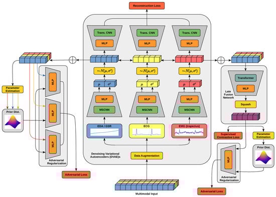
Figure 1. The general architecture of the MM-SCAAE pretraining model for fusing the information from multi-sensor input data into a global object representation. A Denoising Variational AutoEncoder (DVAE) per input modality acts as a core component (center), which fosters the learning of an expressive latent space. The latent representation spaces are regularized by separated adversarial networks and a common fusion network. The adversarial regularization (left) aligns the output space of each encoder with a shared prior distribution type but individually adapts the distribution parameters. The late fusion network (right) aggregates the unimodal encodings into a global representation space with class partitions induced by the supervised contrastive objective. The global latent space is also regularized by an adaptive prior distribution. The processing course of the three displayed input modalities is highlighted through the individual colors of blue, yellow and (light) red.

Our proposed pretraining framework is best understood as a reformulation of the well-known variational lower bound [20,21] with a modified regularization ${\mathcal{R}}_{\mathrm{Latent}}$ of the latent representation space:

$${\mathbb{E}}_X\left[-log{p}_{\theta }\left(X\right)\right]\le {\mathbb{E}}_X\left[{\mathcal{L}}_{\mathrm{Recon}.}^{\prime }+\underset{{\mathcal{R}}_{\mathrm{Latent}}}{\underbrace{({\mathcal{R}}_{\mathrm{Adv}.}+{\mathcal{R}}_{\mathrm{Con}.}}})\right]$$

(1)

where ${\mathcal{L}}_{\mathrm{Recon}.}^{\prime }$, ${\mathcal{R}}_{\mathrm{Adv}.}$ and ${\mathcal{R}}_{\mathrm{Con}.}$ refer to the denoising reconstruction loss, the adversarial regularizations and the supervised contrastive loss, respectively. Here, $p_{\theta }\left(X\right)$ describes the maximum likelihood estimate over the true data-generating distribution $p_{\mathrm{data}}$, and the expectation over the training data is expressed as ${\mathbb{E}}_X={\mathbb{E}}_{X\sim p_{\mathrm{data}}}$. In the following, we stepwise construct the mathematical framework of Equation (1) by elaborating each model component and elucidating its integration into the overall concept.

2.2. Variational Autoencoder

A Variational AutoEncoder (VAE) [20,21] introduces a stochastic encoder component $q_{\varphi }\left(Z\right|X)$ into the classic autoencoder [22] framework for maximizing the Variational Lower Bound (VLB) in order to approach the true data distribution $p_{\mathrm{data}}\left(X\right)$ via the maximum likelihood estimate over $p_{\theta }\left(X\right)$:

$${\mathbb{E}}_X\left[log{p}_{\theta }\left(X\right)\right]\ge {\mathbb{E}}_X{\mathbb{E}}_{q_{\varphi }\left(Z\right|X)}\left[log{\displaystyle \frac{p_{\theta }(X,Z)}{q_{\varphi }\left(Z\right|X)}}\right]=\mathrm{VLB}.$$

(2)

Here, the model parameters comprise $\theta =\{\varphi ,\psi \}$, and are manifested within the nonlinear encoder $q_{\varphi }\left(Z\right|X)$ and decoder $p_{\psi }\left(X\right|Z)$ components, which are usually realized as neural networks. As a unique characteristic of the VAE, its encoder emits learned parameters for a locally centered distribution around the evidence—supplied by the input sample—from which latent representations are stochastically drawn using the reparameterization trick [20,21]. The multivariate Gaussian is typically chosen with predicted mean and log-variance vectors by the encoder. At the time of inference, expectation of the emitted distribution acts as deterministic encoder output. The VLB can be rewritten as a composite objective of the model’s reconstruction ability ($-{\mathcal{L}}_{\mathrm{Recon}.}$) and the prior distribution alignment ${\mathcal{R}}_{\mathrm{Prior}}$ with the latent encoding space, i.e.,

$$\mathrm{VLB}={\mathbb{E}}_X[\underset{-{\mathcal{L}}_{\mathrm{Recon}.}}{\underbrace{{\mathbb{E}}_{q_{\varphi }\left(Z\right|X)}\left[log{p}_{\psi }\left(X\right|Z)\right]}}-\underset{{\mathcal{R}}_{\mathrm{Prior}}}{\underbrace{D_{\mathrm{KL}}\left(q_{\varphi }\left(Z\right|X)\left|\right|q\left(Z\right)\right)}}]$$

(3)

where $D_{\mathrm{KL}}(·||·)$ stands for the Kullback-Leibler (KL) divergence between two regarded distributions. Proofs for Equations (2) and (3) are provided in Appendix A. Often, a concrete prior distribution $q\left(Z\right)$ is chosen. However, we vote for a relaxed formulation that solely specifies the distribution type and adaptively determines the distribution parameters during model training. This proceeding is inspired by previous VAE deliberations that either refrain from a prior distribution [23] or approximate a data-dependent prior using moving averages with momentum [12,24]. An isolated consideration of the $D_{\mathrm{KL}}$-regularizer ($={\mathcal{R}}_{\mathrm{Prior}}$) implies a penalty on the mutual information $I(X,Z)$ between the evidence X and the latent variables Z, which can be interpreted as information processing costs that can be optionally weighted with an inverse temperature [12,24,25,26]. In this context, the optimal prior is determined via marginalization $q^{\ast }\left(Z\right)={\mathbb{E}}_X\left[q_{\varphi }\left(Z\right|X)\right]={\sum }_X{q}_{\varphi }\left(Z\right|X)p_{\mathrm{data}}\left(X\right)$ over the complete evidence [24,25,26,27]. Interestingly, the equally weighted composition of the reconstruction ability and the $D_{\mathrm{KL}}$-regularizer instead maximizes the mutual information, i.e., $\mathrm{VLB}=I(X,Z)+\mathrm{const}.$ (see last proof in Appendix A), leading to seemingly contradictory interpretations. However, $\beta$-VAE [28] makes clear that the application-specific balancing between reconstruction ability and prior distribution alignment forms a key ingredient in establishing a trade-off between competing optimization goals. A natural choice for an adaptive latent distribution represents the multivariate Gaussian $\mathcal{N}\left(X\right|0,{\sigma }^2\mathbb{I})$ with zero-mean and estimated variance ${\sigma }^2$ according to (cf. [12]):

$${\sigma }_{t+1}^2=(1-{\displaystyle \frac{1}{\tau }}){\sigma }_t^2+{\displaystyle \frac{1}{\tau }}\mathrm{Var}\left[q_{\varphi }\left(Z\right|X_t)\right],$$

(4)

where ${\sigma }_t^2=\mathrm{Var}\left[q_t\left(Z\right)\right]$ at time step t and the hyperparameter $\tau$ defines the sensitivity to value changes. Each modality owns an exclusive variance estimate. Since the scaling of features immensely influences the severity of their discrimination [29], we average variance updates over all feature dimensions to prevent overfitting.

2.2.1. Bernoulli Denoising Criterion

Denoising AutoEncoders (DAE)s [30,31] extend traditional autoencoders by recovering the original state of stochastically corrupted inputs for encouraging model robustness against input noise. In the context of Denoising Variational AutoEncoders (DVAE)s, the conventional VLB needs an update in terms of noisy input consumption. According to [32], we define the noise-injected encoder component as follows:

$${\tilde{q}}_{\varphi }\left(Z\right|X)=\int q_{\varphi }\left(Z\right|\tilde{X})p_{\pi }\left(\tilde{X}\right|X)d\tilde{X}$$

(5)

by means of a predefined corruption distribution $p_{\pi }\left(\tilde{X}\right|X)$, which entails the Denoising Variational Lower Bound (DVLB):

$${\mathbb{E}}_X\left[log{p}_{\theta }\left(X\right)\right]\ge {\mathbb{E}}_X{\mathbb{E}}_{{\tilde{q}}_{\varphi }\left(Z\right|X)}\left[log{\displaystyle \frac{p_{\theta }(X,Z)}{q_{\varphi }\left(Z\right|\tilde{X})}}\right]=\mathrm{DVLB}.$$

(6)

The denoising criterion integrates to an equivalent optimization objective formulation as in Equation (3), but shapes stochastic latent neighborhoods around original samples:

$$\mathrm{DVLB}={\mathbb{E}}_X[\underset{-{\mathcal{L}}_{\mathrm{Recon}.}^{\prime }}{\underbrace{{\mathbb{E}}_{{\tilde{q}}_{\varphi }\left(Z\right|X)}\left[log{p}_{\psi }\left(X\right|Z)\right]}}-\underset{{\mathcal{R}}_{\mathrm{Prior}}^{\prime }}{\underbrace{D_{\mathrm{KL}}\left(q_{\varphi }\left(Z\right|\tilde{X})\left|\right|q\left(Z\right)\right)}}].$$

(7)

As mentioned in [31], optimizing against the DVLB is equivalent to maximizing the mutual information $I(X,Z)$ between the uncorrupt data X and the latent factors Z from an information-theoretic perspective. Proofs for the statements in Equations (6) and (7) and for the maximization of mutual information are given in Appendix A. It is important to note that the positive effects on model robustness resulting from denoising regularization directly depend on the application-specific sensitivity to certain noise levels [32]. Although additive Gaussian noise is usually favored as default input corruption, we declare Bernoulli-based feature selection as a universal variant of noise injection. Due to the manipulation of concrete feature values using additive Gaussian noise, we argue that an appropriate trade-off between beneficial denoising and potential signal degeneration is less intuitive to find and frequently requires specific domain knowledge. On the contrary, a Bernoulli corruption distribution $p_{\pi }\left(\tilde{X}\right|X;\mathcal{B}\left(\pi \right))$ solely influences feature existence and can be easily implemented via Dropout [33]. In particular, theoretical analysis in [32] at least indicates that introducing further stochastic layers into the encoder network can tighten the VLB.

2.2.2. Adversarial Regularizer

An Adversarial AutoEncoder (AAE) [34] replaces the $D_{\mathrm{KL}}$-regularizer of the VAE with a competitive network to discriminate between the learned posterior and the desired prior by means of random samples drawn from both distributions. According to the conventional Generative Adversarial Network (GAN) [35] training procedure, this can be realized as alternate optimization leading to the latent regularization

$${\mathcal{R}}_{\mathrm{Adv}.}=-log\left(4\right)+2·D_{\mathrm{JS}}\left(q_{\varphi }\left(Z\right|X)\left|\right|q\left(Z\right)\right)$$

(8)

for the encoder network (also known as the generator), given that the discriminator is optimal. Here, $D_{\mathrm{JS}}(·||·)$ corresponds to the Jensen-Shannon (JS) divergence $D_{\mathrm{JS}}\left(p\left(X\right)\right|\left|q\left(X\right)\right)={\displaystyle \frac{1}{2}}\left[D_{\mathrm{KL}}\left(p\left(X\right)\left|\right|{\displaystyle \frac{p\left(X\right)+q\left(X\right)}{2}}\right)+D_{\mathrm{KL}}\left(q\left(X\right)\left|\right|{\displaystyle \frac{p\left(X\right)+q\left(X\right)}{2}}\right)\right]$, which symmetrizes the KL divergence of the distributions $p\left(X\right)$ and $q\left(X\right)$ with their normalized and equally weighted mixture as the reference distribution. In particular, the mixture reference distribution smooths the regularization loss for the case of heavy deviations in $q_{\varphi }\left(Z\right|X)$ from small values in $q\left(Z\right)$. Both of these adjustments secure a more sophisticated distribution discrimination criterion compared to the classic $D_{\mathrm{KL}}$-regularizer. As unique property, the adversarial regularizer potentially has access to universal function approximation capabilities for distribution discrimination. This property promotes full space exploitation of the target/prior distribution. In contrast to this, the non-parametric $D_{\mathrm{KL}}$-regularizer could easily be fooled with the use of sample repetition or punctual space exploitation. A descriptive demonstration of this phenomenon can be found in the primary AAE paper [34]. Due to the inclusion of the previously described Bernoulli denoising criterion, our framework builds upon Denoising Adversarial AutoEncoders (DAAE)s [36] with probabilistic encoders (borrowed from VAEs) as central components. There exists empirical evidence that DAAEs can improve classification performance on downstream tasks and coherence in sample synthesis after one additional iteration [36].

2.3. Supervised Contrastive Objective

Supervised Adversarial AutoEncoders (SAAE)s [34] make use of available label information to partition latent representations in accordance with a priori class memberships. We propose a novel implementation of the SAAE framework by incorporating a Supervised Contrastive (SupCon) training objective for indirectly backpropagating class association from a common fusion network through all unimodal encoders. For this purpose, we design an adjusted similarity measure for latent representations, present the used SupCon loss and develop a loss variant for class-ordinality injection. The effectiveness of our general SAAE implementation is empirically verified with descriptive results for the MNIST [37,38] dataset, which are provided in Appendix D.

2.3.1. Similarity Measure

The $\mathrm{squash}\left(\mathbf{x}\right)$ function [19] is regularly used in the context of Capsule Networks (CapsNet)s [19,39] as a special activation function to scale the second norm $\left|\right|·\left|\right|$ of a vector output $\mathbf{x}$ to be in the range of $[0,1]$, while preserving original vector orientation. A typical use case for squash normalization is the interpretation of vector magnitude as the existence probability of an observed entity and vector elements as the entity instantiation parameters [19]. The entanglement of distributed representations (i.e., capsules [40]) with their entity existence probabilities improved model performance in previous work concerning text classification [41] and image recognition [39]. Consistently, we enhance traditional contrastive learning by involving model prediction confidence in latent representations into the similarity consideration between input samples using the squash function [19]:

$$\widehat{\mathbf{x}}={\mathrm{squash}}_{\alpha }\left(\mathbf{x}\right)={\displaystyle \frac{\alpha +{\left|\right|\mathbf{x}\left|\right|}^2}{1+{\left|\right|\mathbf{x}\left|\right|}^2}}{\displaystyle \frac{\mathbf{x}}{\left|\right|\mathbf{x}\left|\right|}},\left|\right|\widehat{\mathbf{x}}\left|\right|\in [\alpha ,1],$$

(9)

where we include the constant $\alpha \in [0,1]$ as a smoothing term. In all of our experiments, we limit the lower bound of vector magnitudes to $\alpha =0.1$ for ensuring numerical stability and fostering faster optimization convergence. This proceeding constitutes a relaxation of the classic contrastive learning constraint based on unit vectors, due to the integration of sample relevance, which attenuates the overestimation of outliers. Incorporating the squash function into the inner product $⟨·,·⟩$ leads to a confidence-aware version of the cosine-similarity

$$s(\mathbf{x},\mathbf{y})={\displaystyle \frac{⟨\widehat{\mathbf{x}},\widehat{\mathbf{y}}⟩+1}{2}}\in [0,1]$$

(10)

between the two vectors $\mathbf{x}$ and $\mathbf{y}$, which we additionally normalize to positive values, with one as the upper bound. A more detailed discussion about the impact of prediction confidence on the defined similarity measure is provided in Appendix B.

2.3.2. $ϵ$–SupInfoNCE Loss

Ref. [42] presented the first SupCon loss that deviated from the self-supervised scheme of attracting augmented versions of an anchor sample and repelling all other samples, by instead accessing predefined labels for class discrimination. The $ϵ$–SupInfoNCE loss [43] can be seen as an advancement of the classical SupCon loss by eliminating the implicit constraint of collapsing same-class instances to a single point and by introducing an $ϵ$-margin hyperparameter for fine-tuning metric-based learning. The $ϵ$–SupInfoNCE loss is defined as follows [43]:

$${\mathcal{R}}_{\mathrm{Con}.}^{\mathrm{Nom}.}=-{\displaystyle \frac{1}{\left|P\right|}}\sum _{i}log\left({\displaystyle \frac{exp\left(s_i^{+}\right)}{exp(s_i^{+}-ϵ)+{\sum }_{j}exp\left(s_j^{-}\right)}}\right)$$

(11)

where $s_i^{+}$ and $s_j^{-}$ indicate the similarity between two latent representations from samples of the same class and from samples of distinct classes, respectively. We adopt the scaling factor $1/\left|P\right|$ from [42] to relate the SupCon loss to the number of positive samples $\left|P\right|$ for each temporary anchor within a batch. Specifically, Equation (11) represents a nominal loss function with regard to multi-class problems by equally weighting distances between differing classes.

2.3.3. Ordinal $ϵ$–SupInfoNCE Loss

An ordinal version of the $ϵ$–SupInfoNCE loss requires an application-specific alignment of the $ϵ$-margin with intrinsic class relationships. In general, this requirement can be formalized in three steps. At first, we state the similarity of a latent representation ${\mathbf{x}}_i^{\left(n\right)}$ relative to the latent representation of a selected anchor sample ${\mathbf{x}}_a^{\left(p\right)}$ as follows:

$$s_i^{\left(n\right)}=s({\mathbf{x}}_i^{\left(n\right)},{\mathbf{x}}_a^{\left(p\right)})$$

(12)

where the superscripts $n,p\in \mathbb{N}$ signify belonging to a certain class through its ordinal label. Here, the case $n=p$ is explicitly included and would indicate a positive sample in terms of the nominal $ϵ$–SupInfoNCE loss. In the next step, we create a training objective specification between two samples from different classes with

$$\{s_j^{\left(n\right)}-s_i^{\left(p\right)}+f_{ϵ}\left(r_{np}\right)\le 0|n\ne p\}\forall i,j$$

(13)

where the function $f_{ϵ}\left(r_{np}\right)$ defines the minimal $ϵ$-margin between both regarded samples based on their absolute class label difference $r_{np}$. The class label difference $r_{np}$ can especially be seen as relative rank distance because of its integer nature. To fulfill the ordinality constraint, $f_{ϵ}(·)$ must be a strictly monotonically increasing function by means of the rank-based distance between classes. Both of these properties are summarized in the following statements:

$$r_{np}=|n-p|,f_{ϵ}\left(x\right)<f_{ϵ}\left(y\right)\forall x<y.$$

(14)

Using the optimization objective in Equation (13), we can devise an ordinality-aligned version of the original $ϵ$–SupInfoNCE loss in the form of

$${\mathcal{R}}_{\mathrm{Con}.}^{\mathrm{Ord}.}=-{\displaystyle \frac{1}{\left|P\right|}}\sum _{i}log\left({\displaystyle \frac{exp\left(s_i^p\right)}{exp\left(s_i^p\right)+{\sum }_{j}exp(s_j^n+f_{ϵ}\left(r_{np}\right))}}\right)$$

(15)

where we omit the parenthesis of the class labels in the superscript for the benefit of a compact notation. The loss derivation of Equation (15) follows the proceeding in [43] and can be seen in Appendix C.

2.4. Mutual Information Constraints

Mutual information regularizations were previously included within hierarchical models to facilitate efficient information processing with limited resources [12,23,24,25,26]. This idea is grounded in the principle of information-theoretic bounded rationality [27], which regards information processing costs as additional factor for decision-making. In view of the disentanglement of latent variables, $\beta$-VAE [28] also suggests the integration of a task-specific weighting on the KL divergence regularization into the classical VAE framework, but still remains with a static prior distribution. Since we prefer adaptive prior distributions in our approach, we can analogously formulate mutual information constraints for the pretraining of our multi-stage pain classification model with the aid of Lagrange multipliers ${\beta }_i\in {\mathbb{R}}^{+}$ as in [12,24,25,26]:

$$\begin{array}{cc}\hfill {\mathcal{R}}_{\mathrm{MI}}^{\mathrm{pre}}& ={\displaystyle \frac{1}{{\beta }_1}}\sum _{i=1}^{C}I(X_i,Z_i)+{\displaystyle \frac{1}{{\beta }_2}}I(V,\{Z_1,..,Z_C\})\hfill \end{array}$$

(16)

$$\begin{array}{cc}\hfill \hspace{1em}\hspace{1em}\hspace{1em}\hspace{1em}\hspace{1em}& ={\displaystyle \frac{1}{{\beta }_1}}\sum _{i=1}^{C}log{\displaystyle \frac{q_{\varphi }\left({\mathbf{z}}_i\right|{\mathbf{x}}_i)}{q_i\left(\mathbf{z}\right)}}+{\displaystyle \frac{1}{{\beta }_2}}log{\displaystyle \frac{p\left(\mathbf{v}\right|{\mathbf{z}}_1,..,{\mathbf{z}}_C)}{p\left(\mathbf{v}\right)}}\hfill \end{array}$$

(17)

where $X_i$ means the random variable of the i-th input channel, $Z_i$ states the corresponding latent representation, and V encapsulates the global entity encoding received from the late fusion network. Although we formulate the partial goal to reduce mutual information based on the adversarial prior regularizations, the $ϵ$–SupInfoNCE loss particularly shapes a lower ($ϵ=0$) or upper ($ϵ\to \infty$) bound on the mutual information [43,44]. These bounds can be further tightened with a proper choice of the $ϵ$-margin [43]. Our motivation behind this composite learning objective is to shift the focus from high-dimensional instance appearance (i.e., reconstruction ability) as a crucial attribute for mutual information toward latent features for class discrimination.

3. Related Work

Autoencoders: Previous work [23] on VAEs advocated for maximizing the log-likelihood of the data distribution without latent regularization against a prior, with the precondition that the approximation ability of the encoder network is sufficient. More recently, a Probabilistic Autoencoder (PAE) [45] has been used to decouple the VAE objectives but formulate a two-stage training of first optimizing solely the reconstruction ability and then learning a bijective mapping to construct a useful latent space using Normalizing Flows (NF)s [46,47]. However, PAEs mainly focus on exact likelihood computation with regard to realistic modeling and generation of data samples, whereas our approach aims to conserve class-discriminative characteristics merely directed by reconstruction ability, allowing for less costly model architectures and training. Sacrificing reconstruction quality in favor of other purposes is not a novelty, for instance, $\beta$-VAE systematically oversizes prior regularization to encourage the disentanglement of latent variables, which potentially eases subsequent classification tasks [28]. Moreover, the clustering technique Class-Variational Learning (CVL) [48] constructs a class-discriminative equivariant latent space by combining the aim of reconstruction ability with the decomposition of sample mixtures using a CapsNet encoder. In an opposite direction, Thiam et al.’s pain assessment model [12] introduced an adaptive prior distribution for latent space regularization based on an exponential running mean of the empirical posterior. We think that this harbors the risk of forward latent space collapse by approaching the mass center of the posterior. Instead, we encourage a latent space alignment with a zero-mean Gaussian but allow the model to iteratively adjust the prior’s mean variance over the latent factors. In general, there is still controversy around weighting autoencoder objectives favoring likelihood/mutual information maximization [23,45,49] or privileging task-specific goal adjustments [24,25,26,28,48], with an ongoing lack of clear guidance.

A common pattern we observe with autoencoder models constitutes the stochastic construction of the latent space with many similar inputs mapped to a few locally stochastic neighborhoods inducing enhanced generalizability and generative abstraction, which can be categorized as Vicinal Risk Minimization [50] strategy. The most straightforward realization of this pattern represents VAE [20,21] with its stochastic encoding and latent space regularization, but also DAE [30,31,32,36] implicitly creates local neighborhoods around its encodings through random input distortions. In fact, even the general concept of bounded rationality shares a similar spirit by penalizing exact bijective relations between original and latent representations [25], which was previously integrated into Thiam et al.’s autoencoder model [12]. In addition to the prominent variational and denoising criteria of autoencoders, our approach establishes a higher-level arrangement of local neighborhoods within class-associated partitions based on the supervised contrastive learning objective.

Information Fusion: The general task of information fusion concerns a superior system which consumes multiple feature streams of possibly variable granularity and learns to extract, combine and route latent information in order to fulfill a single or several objectives. This problem formulation is strongly related to the task of meta-learning [24,26], where sample-wise information from a multimodal dataset, consisting of several single-task datasets, must be extracted, optionally combined and routed to the proper expert agent system(s). In particular, we will propose dedicated data augmentation methods (see Section 4.3) to artificially constitute a meta-learning dataset during training with the aid of modality dropout and replacement operations. As a consequence, we enrich the major task of pain classification with the implicit sub-tasks of robust and resilient information fusion. Also note that the multi-task latent space with subsequent selection network in [24,26] for the probabilistic assignment to expert agents can be directly interpreted as a late fusion network.

Contrastive learning was previously adopted for the task of unsupervised information fusion by, among others, aligning multi-channels of visual entities [51,52], exploiting temporal dependencies between concurrent videos of varying viewpoints [53], understanding scenes of 3D point clouds [54] and performing multimodal sentiment analysis [52]. Concerning the processing of time-series data, other works addressed representation learning for robust classification [55] and multivariate anomaly detection [56]. Another approach conducted SupCon learning for multimodal information fusion with regard to the combination of audio-visual channels with textual input to shape a global representation [57]. Note that the terminology of multiview samples in the context of contrastive learning has the ambiguous meaning of $\left(1\right)$ multi-channel inputs of the same data instance [51,53,54] or $\left(2\right)$ data augmentations to enlarge the batch size for contrastive loss computation [42,43]. In our pain classification approach, we characterize distinct biophysiological signals for measuring pain reaction as multimodal data to emphasize their sensory variety, which is a consistent interpretation with recent work [57]. Hence, we link multiview to its $\left(2\right)$ meaning. Related to our focus on class-discriminative feature extraction and combination, Tian et al.’s contrastive framework [51] aims to filter solely channel-invariant entity information from the output of channel-specific encoders. Liu et al.’s TupleInfoNCE [52] training procedure pursues the goal of intensifying the combined usage of modality information based on data augmentation for the creation of positive samples and a modality replacement operation for hard negative mining. Both positive and negative sample generation are parameterized and follow an auxiliary update cycle [52]. Since the task of pain recognition traditionally provides scarce training data and therefore requires time-consuming Leave-One-Subject-Out cross validation, involving comprehensive hyperparameter search circles is usually unfeasible. From a technological perspective, Mai et al.’s work [57] represents the approach most akin to our general multimodal fusion framework by applying SupCon training on lately fused entity encodings and by performing diverse data augmentation techniques to cope with a limited amount of labeled data. The key difference between both approaches lies in the role of the modalities. In the work of Mai et al. [57] (and also in [52]), each modality means an essential part of a specific object, while our model instead maps multiple modalities to the identical object class, allowing for intended sensory redundancy. The assumed supplementary relationship of sensory measurements in pain reaction can be characterized as crossmodal embedding [52], where modalities contribute to a majority voting for pain class prediction. In particular, the sensory redundancy improves failure resistance at runtime, conditions representation learning on all sensory inputs during training and allows for the extension of measurement equipment. Unlike to Mai et al. [57], we prefer a single but more complex fusion network as trade-off between modeling capacity and computational efforts. Yu et al. [56] jointly trained an autoencoder architecture with an adversarial feature discrimination objective instead of a traditional contrastive loss in order to detect anomalies within multivariate time series. Despite the novelty of adversarial contrastive learning, their approach lacks mathematical foundations and dedicated experiments that explain its relationship to theoretically grounded contrastive loss functions such as $ϵ$–SupInfoNCE.

Pain Recognition: In the pain recognition literature there are already various works on classifying the pain intensities of the BioVid dataset. These works propose methods that build upon facial expressions obtained from video recordings [3,4], use measured biopotentials [3,5,6,7,8] or combine all of those modalities together [3,9,10]. Regarding the used methodology, early works [3,5,9,10,11] rely on comprehensive preprocessing schemes for producing handcrafted features and employ rather simple machine learning methods, i.e., random forests, logistic regression and linear Support Vector Machines (SVM)s, for executing classification tasks.

Thiam et al. [6] presented the first approach which substituted the engineering of handcrafted features with Convolutional Neural Networks (CNN)s and restricted signal preprocessing solely to dimensionality reduction. More precisely, they constructed modality-specific CNN-based feature extractors for biophysiological input signals and tested them in unimodal and multimodal classification settings. In the multimodal setting, they used a linear network layer for late fusion. The experimental results revealed that modalities significantly differ in their contribution to solving the task; in addition, multimodal fusion models may suffer from inconsistencies between distinct modalities. Preceding their work, Thiam et al. [7] designed a denoising convolutional autoencoder with a gating network for late fusion, which were jointly trained with the pain classification objective. More recently, Thiam et al. [12] enhanced their previous multimodal fusion model by enlarging the gating network with the aid of an attention module and by involving VAEs with adaptive prior distributions. The key difference between these models and our approach lies in the transformer architecture of MM-SCAAE’s late fusion network, and in the metric-learning SupCon regularization, which merely aligns with the downstream task. Utilizing the well-known high capacity of a transformer architecture for late fusion in order to detect interdependencies between feature vectors allows for avoiding the engineering of sophisticated gating mechanisms. The combination of the late-fusion transformer network with the SupCon loss should facilitate the robust representation learning known from the general SAAE framework.

In the most recent works, the focus has shifted from generic multimodal methods to complex unimodal models. Lu et al. [13] proposed a highly specialized encoder architecture dedicated to one specific biophysiological modality consisting of a MSCNN, a squeeze-and-excitation residual network and a transformer network. Li et al. [14] refined this model through the addition of a multi-scale cross-attention mechanism to the transformer encoder. The major weakness of both approaches originates from their highly complex feature extraction networks and the fixation on a single pain-reaction channel. This means that their models are barely scalable to multi-sensor systems, and do not provide a potential fusion functionality for multiple input signals. The second aspect is especially controversial in a sensitive environment such as medical care.

To enhance the robustness of automated pain assessment in terms of sensor failure tolerance and to increase their trustworthiness in pain-level predictions, we prefer a multimodal pain recognition system based on several biopotentials. For this reason, our generic MM-SCAAE framework supports the straightforward expansion to auxiliary biophysiological measurements, with the inherent option to tailor unimodal autoencoders to specific input types.

4. Results

4.1. BioVid Dataset

The Biopotential and Video (BioVid) Heat Pain Database (Part A) [1,2,3] is a publicly available pain classification dataset. It comprises time series of biophysiological signals combined with frontal video recordings (including depth data) of facial expressions gathered from a controlled experiment of external pain stimulation with 90 study participants. Since the data collection of 3 subjects suffers from missing values due to technical problems, we only concentrate on the remaining 87 individuals, as is common in the literature. The distribution of individuals per age group and sex is approximately balanced. Pain stimuli were induced as heat application on the skin of the right arm using four discrete heat intensities representing distinct pain levels. The lowest and the highest pain levels were determined during an initial calibration phase per patient. In this calibration phase, the temperature induced by the heat-application device was constantly increased and patients were asked to report their lower-bound pain threshold (i.e., if pain perception starts) and upper-bound pain tolerance (i.e., if perceived pain is unacceptable). The pain levels consist of the participant’s self-reported lower-bound pain threshold ($T_1$) and upper-bound pain tolerance ($T_4$) with two equally distant intermediate levels ($T_2$ and $T_3$), which are proportionally mapped to the respective heat intensities. During the experiment, each subject experienced a randomized sequence of 80 heat intensities composed of 20 stimuli per pain level. After reaching the required temperature of a pain level, each heat stimulus was held for 4 s. Between successive stimuli, heat emission randomly paused for $t_{\mathrm{pause}}\in [8,12]$ s plus the needed time for cooling down the heat module to the baseline temperature of 32 °C. In addition, baseline data without pain ($T_0$) were extracted from the pauses to obtain a time span with same magnitude to the 20 stimuli per pain level. Each sample captures a period of 5.5 s. The biophysiological signals encompass biopotentials measured via Electrocardiogram (ECG), Electrodermal Activity (EDA)/Galvanic Skin Response (GSR) and Electromyography (EMG) at the trapezius muscle. The temporal synchronization between the measurements was ensured with the aid of a specialized medical device for multimodal data acquisition. In this paper, we restrict our experiments to the multimodal recognition of the four ordinal pain levels in relation to the no-pain baseline based on these biophysiological signals.

4.2. Pain Recognition Task

We formalize the task of pain recognition as a supervised learning scenario of binary classification where emerging pain intensities ($T_1$, $T_2$, $T_3$, $T_4$) need to be separated from the patient’s normal state ($T_0$). For this purpose, a certain number C of the patient’s biopotentials are periodically monitored over a predefined time span S, resulting in a multimodal sample $X\in {\mathbb{R}}^{C\times S}$. The training data of each pain recognition task comprises the normal state samples ${\left\{(X_i,T_0)\right\}}_{i=1}^N$ and the pain episode samples ${\left\{(X_j,T_k)\right|k\ne 0\}}_{j=1}^N$ of pain intensity $T_k$. As a performance evaluation regime for each pain recognition task, the Leave-One-Subject-Out (LOSO) [4,6,7,8,11,12] cross validation is adopted. This means that for each run, the model performance is tested on a specific patient that was excluded from the training procedure. Finally, the overall model performance is determined as average over all LOSO runs. The practical relevance of the individual pain recognition tasks increases with the relevant pain intensity. Since the discrimination between neighbored pain intensities to date constitutes a notably challenging problem, it is common in the present literature to focus on the above binary classification tasks for evaluating a model’s performance.

4.3. Data Preprocessing and Augmentation

This section chronologically presents the implemented data preprocessing and augmentation pipeline for the task of pain recognition based on the multimodal biophysiological measurements from the BioVid heat pain database.

4.3.1. Instance-Based Normalization

We conduct min-max normalization channel-wise for each multimodal sample $X\in {\mathbb{R}}^{T\times C}$, with C feature channels and a sequence length of T, over its temporal dimension by

$${\tilde{x}}_{i,c}\left(t\right)={\displaystyle \frac{x_{i,c}\left(t\right)-min\left({\mathbf{x}}_{i,c}\right)}{max\left({\mathbf{x}}_{i,c}\right)-min\left({\mathbf{x}}_{i,c}\right)}}\in [0,1],$$

(18)

where ${\mathbf{x}}_{i,c}\in {\mathbb{R}}^T$ refers to the complete time series of the c-th channel from the i-th sample, and $x_{i,c}\left(t\right)$ denotes the single feature at time step t. Hence, we obtain a reasonable feature range per sample without harming the time-dependent structure. This sample-wise normalization strategy is inspired by Layer Normalization (LN) [58], which is regularly applied on layer-wise neural activities in conjunction with sequential data. Contrary to LN, we refrain from zero-mean and unit-variance normalization and omit the final reparameterization step of explicit signal re-scaling and re-shifting. Apart from this single instance-based normalization step applied to all modalities, no additional preprocessing is conducted. In the following, the data augmentation pipeline for the training process is presented.

4.3.2. Random Crop

As a straightforward data augmentation technique, we apply random cropping to each input sequence. When the i-th sample $X_i\in {\mathbb{R}}^{T\times C}$ with length T and C channels is drawn from the training set, a random window with fixed length t is selected to constitute a multi-channel augmented sequence

$${\tilde{X}}_i={\left(X_i\right)}_{s\le j\le s+t},s\sim \mathcal{U}(0,T-t),$$

(19)

where j states the selected time frame, and s describes the shift from the start of the input sequence. The window shift s is sampled from the uniform distribution bounded by the minimal value of zero and the maximal value of $T-t$. Specifically, we clip windows of length $t=2688$ from input sequences of original length $T=2816$. Taking into account the sample rate of 512 per second within the recorded signals from BioVid, we allow for maximal shifts of 250 ms. At the time of model inference, the window selection is deterministic, setting s to the rightmost position, i.e., $s=T-t$. The rationale behind this proceeding derives from the expectation of occurring latency in biophysiological reactions on pain events. Temporal multi-channel alignment has been proven to form strong self-supervisory signals for robust learning of dynamic processes [53]. Previous approaches performed similar temporal cropping operations [6,7,12].

4.3.3. Modality Replacement

To facilitate the training of a patient-invariant pain classification model, we randomly replace each modality from a regarded sample with the respective modality of other samples from the identical pain class. Therefore, the process of augmenting the i-th sample $X^{(i,k)}\in {\mathbb{R}}^{T\times C}$ (with C channels and T features) belonging to class k can be mathematically described as

$${\tilde{X}}^{(i,k)}={\{(1-\delta ){\mathbf{x}}_c^{\left(i\right)}+\delta {\mathbf{x}}_c^{\left(y\right)}|{\mathbf{x}}_c^{\left(y\right)}\sim {\mathbf{X}}_B^{\left(k\right)};\delta \sim \mathcal{B}\left(\pi \right)\}}_{c=1}^C$$

(20)

where $\delta \in \{0;1\}$ induces a modality replacement received from a Bernoulli distribution $\mathcal{B}\left(\pi \right)$, and ${\mathbf{x}}_c^{(·)}$ means the c-th channel of a sample from class k within the batch ${\mathbf{X}}_B^{\left(k\right)}$. Throughout our experiments, we have chosen a fair coin flip probability (i.e., $\pi =0.5$) for substituting feature channels. As a beneficial side-effect, modality replacement artificially expands the small training corpus of BioVid with regard to individual patients. Note that the modality replacement operation was already used in prior work [52,57] to produce hard negative samples for multimodal contrastive learning. This is opposed to our modality replacement variant, which identifies the interchangeability of sensory measurements within the same pain class as a substantial training target to engender unbiased representation learning.

4.3.4. Modality Dropout

Finally, we establish the task-specific data augmentation of modality dropout [52], which randomly disables single modalities according to

$$\tilde{X}=X(\mathbb{I}\odot \mathbf{d}),\mathbf{d}={\{d_c\sim \mathcal{B}\left(\pi \right)\}}_{c=1}^C,$$

(21)

where a sample $X\in {\mathbb{R}}^{T\times C}$ with C channels and T temporal features is transformed using the column-wise product of the identity matrix ${\mathbb{I}}_{C\times C}$ and the dropout vector $\mathbf{d}$. The elements of $\mathbf{d}$ are drawn from a Bernoulli distribution $\mathcal{B}\left(\pi \right)$. Again, we use an equal probability (i.e., $\pi =0.5$) for switching off individual feature channels. In the extreme case of eliminating all modalities by chance, we simply turn on all channels instead. The motivation behind modality dropout is three-fold: Firstly, the model is enforced to focus on each modality for preventing the known problem of overestimating single feature channels [52] and promoting a more contextualized information fusion. Especially in the case of BioVid’s biophysiological recordings, empirical evidence suggests that the EDA measurement appears to be significantly more informative than the ECG and EMG modalities [5,6,9,10,11], which could narrow a model’s perspective. Secondly, in the practical application of pain assessment, an invariant, or at least a resilient, model prediction is highly desirable to compensate for partial outages of sensors. Thirdly, this data augmentation strategy promotes efficient model extensibility by means of connecting auxiliary sensors with reduced training cost, due to the reuse of frozen autoencoders which have already learned to align their encoded representations with the associated pain class. Expanding the scope of modalities for an object class can particularly strengthen representation learning [51,53].

4.4. Network Components

The generic MM-SCAAE pretraining model in Figure 1 requires the specification of all network components for the task of pain classification. Hence, we provide in Figure 2 the implementation details on the variational encoder, the decoder and the late fusion network. Since previous works [13,14] on pain classification using the EDA signal from BioVid empirically validated the effectiveness of MSCNN [15,16] for temporal feature extraction, we incorporate an analogous MSCNN into our variational encoder. In particular, we follow the basic MSCNN structure defined in [15] of parallel convolutional layers with a subsequent fully connected projection head for harmonized feature concatenation. Consistent with [13,14], we establish three scales by applying different-sized convolutional kernels on the raw sensory time series. However, we expand the smallest time window from 0.1 s to 0.5 s in order to better account for the latency in biophysiological reactions and to significantly reduce computational efforts. In Figure 2, we state temporal convolutional layers (Conv1D)s with the used activation function, the number of filters and the strides (as downsampling (/x) or upsampling (*x) factor). The first downsampling factor c of the MSCNN is $10\%$ of the window size. Apart from the first Conv1D, all convolutional layers within the encoder have a kernel size of 10. A fully connected layer (Dense) is characterized by its activation function and its neuron count. The application of the Gaussian Error Linear Unit (GELU) [59] activation function within the encoder can induce positive effects on the model’s generalizability [13]. The encoder emits per feature dimension a Gaussian distribution centered around the latent representation by predicting the distributions’ mean $\mu$ and variance ${\sigma }^2$.

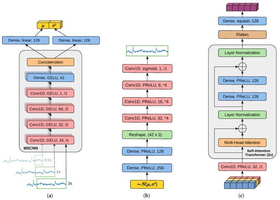
Figure 2. Implementation of MM-SCAAE’s model components for the task of multi-sensor pain classification. (a) Variational encoder component of each unimodal autoencoder. The encoder extracts features of varying granularity with window size $w\in \{0.5,1,2\}$ in seconds using a Multi-Scale Convolutional Neural Network (MSCNN) and produces parameter estimates for a local Gaussian distribution. (b) Denoising decoder component of each unimodal autoencoder. The decoder receives a stochastically sampled latent representation drawn from the local Gaussian distribution predicted by the encoder, and reconstructs the uncorrupt input. (c) The late fusion network aggregates the multimodal information into a global object representation via two sequential self-attention transformer layers. Within each subfigure, identically colored network layers share the same layer type.

The decoder network draws a sample from the Gaussian and reconstructs the original input. The decoder is composed of an MLP and a subsequent transposed convolutional network (cf. [17]) with kernel sizes $\{10,10,10,1\}$. The late fusion network at first creates distinct views of the modality encodings (with kernel size of 5), and then applies two sequentially appended self-attention transformer layers [18] (with three multi-head attention heads) to determine a global object representation. Finally, the global object vector is normalized to a magnitude in range of $[0.1,1]$ via the squash function from Equation (9). Except for the output layers, both the decoder and the fusion network conduct the Parametric Rectified Linear Unit (PReLU) [60] activation function with linear initialization. Rectified linear units foster sparsity in neural activity, which may mitigate overfitting problems [16]. Moreover, the adaptivity of PReLU, in combination with its linear initialization, generally accelerates solution space exploration and resulting training progress [29]. The simple architecture of each adversarial network consists of three Dense layers with $\{256,128,1\}$ neurons per layer. Both hidden layers apply PReLU, while the output layer uses the logistic sigmoid. After pretraining the MM-SCAAE model, the DVAEs and the late fusion network are extracted and frozen in order to train a classifier network on top of the global object representations. The classifier has a 128-unit Dense layer with PReLU activation and a two-unit Dense output layer with softmax activation for pain class prediction.

4.5. Global Setup

We implemented our experiments in the programming language Python [61] (version: 3.12.8) using the machine learning library Keras [62] (version: 3.4.1), with Tensorflow [63] (version: 2.17.0) as backend. If parameters are not explicitly defined below, Tensorflow’s default parameter setting is used. Apart from output layers, each network layer integrates Batch Normalization [64] before applying the activation function. In addition, each layer conducts Dropout [33] with a probability of $0.2$ on incoming signals. As a gradient descent optimizer for all training procedures, we utilize AdamW [65], which equips the classic Adam [66] algorithm with proper weight decay. In addition, AdamW is initialized with a learning rate of $0.001$, and the AMSGrad [67] option is activated for enhancing training convergence [29].

The further training configuration comprises a batch size of 128 and training epochs of $\{50,10\}$ for pretraining and classifier optimization, respectively. As a prior distribution type for adversarial regularization, a zero-mean Gaussian with adaptive variance is used (see Section 2.2). Each Gaussian is initialized as standard normal distribution (i.e., with variance ${\sigma }^2=1.0$). The adaptive variance per adversarial regularizer is repeatedly estimated by calculating the empirical variance over the respective batch of latent representations during the forward propagation in each training step. We empirically choose a momentum factor of ${\displaystyle \frac{1}{\tau }}=0.01$ in Equation (4) to ensure a relatively stable variance estimation for proper optimization. This cumulative variance estimation allows for the full description of the Gaussian prior distribution for adversarial loss computation. For balancing adversarial training, especially at the beginning, we add noise $\sim \mathcal{N}(0,0.05)$ to the target logits of the adversarial networks. Following [42,43], we use a temperature value of $\tau =0.1$ in each exponential expression, i.e., $exp(·/\tau )$, of the SupCon losses. The reconstruction loss of the autoencoder model is implemented as Mean Squared Error (MSE). Although we equally weight all pretraining objectives, we observed in preliminary tests that MSE rapidly diminishes after a few epochs, leading to a prevalence of latent regularization, similarly to $\beta$-VAE. To control for the uncertainty in pain classes caused by the measurement of only a small fraction of biophysiological reactions, we include label smoothing [68] with a factor of $0.3$ for non-target classes during classifier training with the cross entropy loss. In Appendix E, we additionally provide a structured list to the global hyperparameters for quick reference.

4.6. Experiments

Within the results of our experiments, model performances are mainly evaluated by means of classification accuracy to ensure a valid comparability to existing pain-recognition methods in the literature. This is necessary since the preferable classification metrics of sensitivity and specificity for evaluating a classifier’s quality in a sensitive domain such as medicine are to date rarely reported in terms of the BioVid dataset. However, we state in our first experiment the relevant classification metrics for appropriately categorizing the resulting performance of our proposed model in the application context of medicine.

4.6.1. Classification Performance

In our first experiment, we aim to evaluate the basic classification performance of our MM-SCAAE pretraining framework for the task of pain recognition. More precisely, we formulate four two-class problems where the no-pain baseline ($T_0$) needs to be separated from the different pain intensities ($T_1$, $T_2$, $T_3$, $T_4$). For this purpose, we consider for pretraining and subsequent classifier training solely the two selected classes per task (i.e., $T_0$ vs. $T_i$). In these two-class scenarios, the MM-SCAAE model employs the nominal $ϵ$–SupInfoNCE loss in Equation (11), with $ϵ=1.0$ as the margin hyperparameter. Table 1 summarizes the performance statistics for the LOSO cross validation per downstream task. Additionally, Figure 3 displays the corresponding Receiver-Operating Characteristic (ROC) curve with the Area Under the Curve (AUC), and the LOSO accuracy distribution per task. In Table 1, we list the classification metrics typically reported in the pain recognition literature in conjunction with BioVid. In particular, the sensitivity and specificity metrics take a special role in assessing a model’s quality for predicting the occurrence of a medical condition. As one would expect, the class separability improves with increasing pain intensity. Note that the final task ($T_0$ vs. $T_4$) has the highest practical relevance for pain recognition, since the linear categorization of the intermediate pain intensities ($T_1$, $T_2$, $T_3$) lack a clear interpretation and medical justification. Our proposed model achieves competitive accuracies and macro-averaged $F_1$-scores for all tasks compared to the existing multimodal pain classification approaches [3,5,6,7,9,10,11,12]. Moreover, our ROC curve plot including AUC values is coherent with prior work [13] on unimodal classification based on the EDA signal. A detailed performance comparison will be provided in the following Section 4.6.4, which relates the capability of MM-SCAAE to previous models.

Table 1. Classification metrics with standard deviations for the LOSO cross validation using two-class pretraining. Except for Cohen’s $\kappa$, all metrics are stated in %. The best value per classification metric is stated in bold.

Task	Sensitivity/Recall	Precision	Specificity	Cohen’s $\mathit{\kappa }$	${\mathit{F}}_1$-Score	Accuracy
$T_0$ vs. $T_1$	$60.64\left(13.20\right)$	$44.83\left(23.71\right)$	$58.09\left(11.44\right)$	$0.15\left(0.19\right)$	$54.99\left(10.85\right)$	$57.61\phantom{0}\left(9.27\right)$
$T_0$ vs. $T_2$	$67.24\left(19.44\right)$	$51.21\left(29.60\right)$	$65.07\left(15.75\right)$	$0.29\left(0.29\right)$	$62.06\left(16.93\right)$	$64.74\left(14.36\right)$
$T_0$ vs. $T_3$	$75.75\left(14.44\right)$	$71.26\left(24.56\right)$	$75.98\left(16.47\right)$	$0.49\left(0.28\right)$	$73.50\left(15.17\right)$	$74.40\left(14.10\right)$
$T_0$ vs. $T_4$	$\mathbf{85}.\mathbf{74}(\mathbf{11}.\mathbf{13})$	$\mathbf{81}.\mathbf{15}(\mathbf{22}.\mathbf{47})$	$\mathbf{84}.\mathbf{96}(\mathbf{15}.\mathbf{52})$	$\mathbf{0}.\mathbf{68}(\mathbf{0}.\mathbf{26})$	$\mathbf{83}.\mathbf{72}(\mathbf{14}.\mathbf{07})$	$\mathbf{84}.\mathbf{22}(\mathbf{13}.\mathbf{12})$

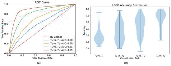
Figure 3. Classification performance evaluation per pain intensity ($T_1$, $T_2$, $T_3$, $T_4$) versus the no-pain baseline ($T_0$). (a) ROC curve and AUC values document the change in performance for various classification thresholds. (b) Violin plot for each LOSO accuracy distribution.

4.6.2. Modality Significance

This post-processing analysis investigates the contribution of each modality to final class prediction. Due to the modality dropout data augmentation technique, we obtain a prediction model resilient against partial sensor failure. Furthermore, modality dropout engenders the tracking of classification performance for all possible sensor combinations during inference. Thus, we evaluate the classification accuracy of the models from our previous experiment in terms of varying sensor availability, as illustrated in Table 2. A sensor can have a value of 0 or 1 meaning off or on, respectively. The results support the suggestion in [13,14] to focus on the EDA modality, since it delivers the strongest overall contribution to effective class separation in the unimodal cases. Nevertheless, our model emphasizes that unimodal evaluation is inferior for each classification task. It is interesting that the EMG modality entails positive or negative effects depending on the downstream task. For the most important task of no-pain baseline $T_0$ versus highest pain $T_4$, each modality accomplishes a significant contribution to class prediction. In particular, we observe that involving only one auxiliary modality to EDA seems to rather degrade accuracy, whereas all three sensors together achieve the highest accuracy for the ($T_0$ vs. $T_4$) task. These observations indicate that the global object representation space formed by the SupCon loss captures nonlinear relationships between the unimodal latent spaces. Finally, the successful composition of a global object space, despite the modality replacement operation, empirically proves effectual patient-invariant learning.

Table 2. Classification accuracy (in %) with standard deviation within the LOSO cross validation for varying sensor availability. Sensor values of 0 or 1 signify sensor state of deactivation or activation, respectively. The best accuracy value per classification task is stated in bold.

Sensors			Tasks
EDA	ECG	EMG	${\mathit{T}}_{\mathbf{0}}\mathrm{vs}.{\mathit{T}}_{\mathbf{1}}$	${\mathit{T}}_{\mathbf{0}}\mathrm{vs}.{\mathit{T}}_{\mathbf{2}}$	${\mathit{T}}_{\mathbf{0}}\mathrm{vs}.{\mathit{T}}_{\mathbf{3}}$	${\mathit{T}}_{\mathbf{0}}\mathrm{vs}.{\mathit{T}}_{\mathbf{4}}$
0	0	1	$49.74\phantom{0}\left(2.65\right)$	$49.94\phantom{0}\left(3.47\right)$	$50.06\phantom{0}\left(6.65\right)$	$53.99\phantom{0}\left(8.34\right)$
0	1	0	$50.40\phantom{0}\left(1.81\right)$	$50.26\phantom{0}\left(2.40\right)$	$51.81\phantom{0}\left(5.78\right)$	$56.70\left(10.89\right)$
0	1	1	$49.37\phantom{0}\left(4.57\right)$	$49.97\phantom{0}\left(3.42\right)$	$52.53\phantom{0}\left(7.19\right)$	$59.86\left(11.85\right)$
1	0	0	$57.07\phantom{0}\left(9.66\right)$	$63.65\left(14.52\right)$	$74.45\left(13.53\right)$	$83.56\left(13.55\right)$
1	0	1	$57.53\phantom{0}\left(9.97\right)$	$64.40\left(14.56\right)$	$74.17\left(13.79\right)$	$83.30\left(13.89\right)$
1	1	0	$\mathbf{57}.\mathbf{70}\phantom{\mathbf{0}}(\mathbf{9}.\mathbf{94})$	$64.08\left(14.25\right)$	$\mathbf{74}.\mathbf{94}(\mathbf{13}.\mathbf{57})$	$83.42\left(14.14\right)$
1	1	1	$57.61\phantom{0}\left(9.27\right)$	$\mathbf{64}.\mathbf{74}(\mathbf{14}.\mathbf{36})$	$74.40\left(14.10\right)$	$\mathbf{84}.\mathbf{22}(\mathbf{13}.\mathbf{12})$

4.6.3. Ordinal-Aware Multi-Class Pretraining

The autoencoder architecture of our model allows for multi-class pretraining. Furthermore, the ordinal SupCon loss formulation enables the injection of domain-specific knowledge via predefined $ϵ$-margin function into the MM-SCAAE pretraining model. Thus, we analyze in our next experiment if the exploitation of further training data from other classes can improve the two-class prediction accuracy. The central motivation behind this proceeding results from the chronic deficit of labeled training data in health care. Specifically, if a pretraining model is able to access information from instances associated with intermediate or surrounding classes, learned representation spaces may profit from smoother transitions for downstream tasks. To test this hypothesis, we conduct multi-class pretraining with the MM-SCAAE model using the classes ${\mathcal{C}}_1=\{T_0,T_2,T_4\}$ and ${\mathcal{C}}_2=\{T_0,T_1,T_2,T_3,T_4\}$. For both class sets we additionally vary the use of nominal and ordinal SupCon loss. The margin hyperparameter for the nominal SupCon loss is chosen as $ϵ=\left(\right|{\mathcal{C}}_i{|-1)}^{-1}$, whereas the ordinal SupCon loss utilizes the margin function $f_{ϵ}\left(r_{ij}\right)=r_{ij}·\left(\right|{\mathcal{C}}_i{|-1)}^{-2}$ with $r_{ij}$ as label difference between the classes $T_i$ and $T_j$. The square exponent within the $ϵ$-margin function helps to balance the magnitudes between the ordinal and nominal SupCon losses. Table 3 illustrates the experimental results for the distinct multi-class pretraining scenarios. Based on the presented results, we can make two observations. Firstly, involving other classes than the selected classes for the downstream task generally lowers model accuracy (except for the task $T_0$ vs. $T_2$). This circumstance can be seen by comparing the accuracies in Table 3 with the former experimental results in Table 1. In addition, accuracy values further reduce from multi-class configuration ${\mathcal{C}}_1$ to ${\mathcal{C}}_2$. Secondly, the ordinal SupCon loss at least slightly degrades model performance compared to the nominal loss version in the most cases. We conclude that each class from BioVid contains a significant noise ratio which accumulates with the inclusion of further classes into the pretraining procedure. Since the multi-class pretraining models gain no benefit from using the ordinal SupCon loss, it implies that there may not exist a gradually linear change in the original representation space of biophysiological pain reactions.

Table 3. Classification accuracy (in %) with standard deviation within the LOSO cross validation using distinct multi-class pretraining scenarios. The best accuracy value per classification task is stated in bold.

Multi-Class Pretraining	SupCon Loss	Tasks
		${\mathit{T}}_{\mathbf{0}}$ vs. ${\mathit{T}}_{\mathbf{1}}$	${\mathit{T}}_{\mathbf{0}}$ vs. ${\mathit{T}}_{\mathbf{2}}$	${\mathit{T}}_{\mathbf{0}}$ vs. ${\mathit{T}}_{\mathbf{3}}$	${\mathit{T}}_{\mathbf{0}}$ vs. ${\mathit{T}}_{\mathbf{4}}$
{$T_0$, $T_2$, $T_4$}	nominal	-	$\mathbf{65}.\mathbf{34}(\mathbf{14}.\mathbf{37})$	-	$\mathbf{83}.\mathbf{39}(\mathbf{13}.\mathbf{44})$
	ordinal	-	$64.66\left(14.79\right)$	-	$83.22\left(13.43\right)$
{$T_0$, $T_1$, $T_2$, $T_3$, $T_4$}	nominal	$57.24\left(10.57\right)$	$63.59\left(13.83\right)$	$\mathbf{72}.\mathbf{13}(\mathbf{13}.\mathbf{88})$	$80.72\left(13.40\right)$
	ordinal	$\mathbf{57}.\mathbf{39}(\mathbf{10}.\mathbf{13})$	$62.39\left(13.34\right)$	$70.26\left(12.28\right)$	$79.89\left(13.49\right)$

4.6.4. Performance Comparison

Table 4 relates the performance of MM-SCAAE on the BioVid dataset to the existing methods. The two separated sections display unimodal approaches and multimodal methods, respectively. Each section is chronologically sorted, starting with the earliest approach. For ensuring valid comparability to the performance of previous pain recognition methods, we only list models which were evaluated by means of the LOSO cross validation. Furthermore, in our experiments we used the standard segmentation scheme of 5.5 s per sample from BioVid [3]. It is important to note that methods marked with (*) cannot be directly compared with the other performance results because of a diverging sample segment size of 4.5 s (example shown in [8]). However, we included these methods for the sake of completeness. The best LOSO cross validation performance is individually emphasized in bold for unimodal and multimodal models. In addition, the best results per section for the model group with diverging segmentation scheme (*) are underlined. In the method descriptions, HCFs stands for HandCrafted Features and CA means Cross-Attention.

Table 4. LOSO cross validation performance comparison of pain recognition models on the BioVid heat pain database using classification accuracy and $F_1$-Score (in %). Values are stated in the format {Accuracy/$F_1$-Score}. The best values are individually emphasized in bold for unimodal and multimodal models per classification task. Additionally, the best values per section for the model group with diverging segmentation scheme (*) are underlined. The (✓) symbol signifies the use of a certain modality for the task of pain recognition.

Method		Modalities				Tasks
		EDA	ECG	EMG	Video	${\mathit{T}}_{\mathbf{0}}\mathrm{vs}.{\mathit{T}}_{\mathbf{1}}$	${\mathit{T}}_{\mathbf{0}}\mathrm{vs}.{\mathit{T}}_{\mathbf{2}}$	${\mathit{T}}_{\mathbf{0}}\mathrm{vs}.{\mathit{T}}_{\mathbf{3}}$	${\mathit{T}}_{\mathbf{0}}\mathrm{vs}.{\mathit{T}}_{\mathbf{4}}$
Unimodal	HCFs + Random Forest [3]				✓	$51.20/$-$\phantom{0.00}$	$54.40/$-$\phantom{0.00}$	$62.90/$-$\phantom{0.00}$	$71.60/$-$\phantom{0.00}$
	HCFs + Logistic Regression * [5]	✓				$54.57/$-$\phantom{0.00}$	$59.40/$-$\phantom{0.00}$	$66.00/$-$\phantom{0.00}$	$74.21/$-$\phantom{0.00}$
	CNN *  [6]	✓				$\underline{61.67}/$-$\phantom{0.00}$	$\underline{66.93}/$-$\phantom{0.00}$	$\underline{76.38}/$-$\phantom{0.00}$	$\underline{84.57}/$-$\phantom{0.00}$
	CNN * [6]		✓			$49.71/$-$\phantom{0.00}$	$50.72/$-$\phantom{0.00}$	$52.87/$-$\phantom{0.00}$	$57.04/$-$\phantom{0.00}$
	CNN * [6]			✓		$49.71/$-$\phantom{0.00}$	$50.29/$-$\phantom{0.00}$	$53.25/$-$\phantom{0.00}$	$58.65/$-$\phantom{0.00}$
	Attention Networks [4]				✓	$\phantom{0.00}$-/-$\phantom{0.00}$	$\phantom{0.00}$-/-$\phantom{0.00}$	$\phantom{0.00}$-/-$\phantom{0.00}$	$69.25/$-$\phantom{0.00}$
	MLP + Random Forest [8]	✓				$59.08/$-$\phantom{0.00}$	$65.09/$-$\phantom{0.00}$	$75.14/$-$\phantom{0.00}$	$84.22/$-$\phantom{0.00}$
	Transformer Encoder [13]	✓				$56.70/55.97$	$68.78/68.79$	$77.41/\mathbf{77}.\mathbf{37}$	$85.56/85.49$
	CA Transformer Encoder [14]	✓				$\mathbf{63}.\mathbf{99}/\mathbf{63}.\mathbf{89}$	$\mathbf{70}.\mathbf{05}/\mathbf{70}.\mathbf{03}$	$\mathbf{78}.\mathbf{24}/77.23$	$\mathbf{86}.\mathbf{21}/\mathbf{85}.\mathbf{85}$
Multimodal	HCFs + Random Forest [3]	✓	✓	✓		$54.90/$-$\phantom{0.00}$	$59.30/$-$\phantom{0.00}$	$65.00/$-$\phantom{0.00}$	$74.10/$-$\phantom{0.00}$
		✓	✓	✓	✓	$54.60/$-$\phantom{0.00}$	$60.00/$-$\phantom{0.00}$	$67.70/$-$\phantom{0.00}$	$77.80/$-$\phantom{0.00}$
	HCFs + Random Forest [9,10]	✓	✓	✓	✓	$\phantom{0.00}$-/-$\phantom{0.00}$	$\phantom{0.00}$-/-$\phantom{0.00}$	$\phantom{0.00}$-/-$\phantom{0.00}$	$83.10/$-$\phantom{0.00}$
	HCFs + Random Forest [11]	✓	✓	✓		$\phantom{0.00}$-/-$\phantom{0.00}$	$\phantom{0.00}$-/-$\phantom{0.00}$	$\phantom{0.00}$-/-$\phantom{0.00}$	$82.73/$-$\phantom{0.00}$
	HCFs + Linear SVM * [5]	✓	✓			$\phantom{0.00}$-/-$\phantom{0.00}$	$\phantom{0.00}$-/-$\phantom{0.00}$	$\phantom{0.00}$-/-$\phantom{0.00}$	$72.20/$-$\phantom{0.00}$
	CNN * [6]	✓	✓	✓		$\underline{61.15}/$-$\phantom{0.00}$	$\underline{66.81}/$-$\phantom{0.00}$	$\underline{76.29}/$-$\phantom{0.00}$	$\underline{84.40}/$-$\phantom{0.00}$
	DAE * [7]	✓	✓	✓		$\phantom{0.00}$-/-$\phantom{0.00}$	$\phantom{0.00}$-/-$\phantom{0.00}$	$\phantom{0.00}$-/-$\phantom{0.00}$	$83.99/$-$\phantom{0.00}$
	Adaptive DVAE * [12]	✓	✓	✓		$\phantom{0.00}$-/-$\phantom{0.00}$	$\phantom{0.00}$-/-$\phantom{0.00}$	$\phantom{0.00}$-/-$\phantom{0.00}$	$84.25/\underline{81.48}$
	MM-SCAAE (ours)	✓	✓	✓		$\mathbf{57}.\mathbf{61}/\mathbf{54}.\mathbf{99}$	$\mathbf{64}.\mathbf{74}/\mathbf{62}.\mathbf{06}$	$\mathbf{74}.\mathbf{40}/\mathbf{73}.\mathbf{50}$	$\mathbf{84}.\mathbf{22}/\mathbf{83}.\mathbf{72}$

In accordance with our former experimental results about modality significance (see Table 2), we observe that the biopotential EDA mainly contributes to the high-quality predictions in previous pain recognition models. Therefore, both Transformer Encoder models which are highly specialized on the EDA modality greatly outperform the other unimodal approaches. Regarding the multimodal methods with standard segmentation, our designed MM-SCAAE model constitutes the new state-of-the-art performance for all binary classification tasks. Moreover, MM-SCAAE’s accuracy is also competitive with the models with diverging segmentation scheme (*), and MM-SCAAE’s $F_1$-score outperforms the formerly reported best value by a significant margin of over two percentage points. Note that the $F_1$-score is typically more expressive and relevant than accuracy in the medical context.

At first glance, our model appears inferior to the unimodal transformer encoders considering both accuracy and $F_1$-scores for all four pain recognition tasks. However, we implemented our MM-SCAAE framework in the experiments with identical autoencoder architectures for arbitrary sensor data in order to satisfy the trade-off between performance and computational effort. In principle, MM-SCAAE offers the capacity to utilize highly specialized feature extractors, such as the EDA-transformer encoder, for certain modalities. Thus, we proposed a universal information fusion architecture for the multi-sensor classification domain of time-series data. In particular, incorporating information from multiple and heterogenous sources is essential for trustworthy decision-making in health care.

Since most works on pain recognition using the BioVid dataset report their classifier quality solely based on classification accuracy, we primarily had to rely on the accuracy metric to ensure valid comparability to existing models in the literature. Although accuracy appears to be a sufficient indicator to compare the performance of different classification models, its expressiveness to evaluate a classifier’s quality in a sensitive domain such as medicine is strongly limited. To account for this circumstance, we additionally state in Table 5 the sensitivity and specificity classification metrics of our model in relation to the state-of-the-art unimodal pain recognition approaches. For the most relevant task of no-pain ($T_0$) versus highest pain ($T_4$), our model achieves a sensitivity on par with the highest-reported value. Directly compared with the Transformer Encoder model, our classifier produces a sound balance between sensitivity and specificity, again reflecting the potency of our MM-SCAAE pretraining framework.

Table 5. LOSO cross validation performance comparison of pain recognition models on the BioVid heat pain database using the sensitivity and specificity classification metrics (in %). Values are stated in the format {Sensitivity/Specificity}. The best metric value per classification task is stated in bold.

Method	Tasks
	${\mathit{T}}_{\mathbf{0}}\mathrm{vs}.{\mathit{T}}_{\mathbf{1}}$	${\mathit{T}}_{\mathbf{0}}\mathrm{vs}.{\mathit{T}}_{\mathbf{2}}$	${\mathit{T}}_{\mathbf{0}}\mathrm{vs}.{\mathit{T}}_{\mathbf{3}}$	${\mathit{T}}_{\mathbf{0}}\mathrm{vs}.{\mathit{T}}_{\mathbf{4}}$
Transformer Encoder [13]	$\mathbf{69}.\mathbf{54}/43.85$	$\mathbf{70}.\mathbf{48}/\mathbf{67}.\mathbf{10}$	$73.16/\mathbf{81}.\mathbf{67}$	$82.70/\mathbf{88}.\mathbf{28}$
CA Transformer Encoder [14]	$64.17/$-$\phantom{0.00}$	$70.05/$-$\phantom{0.00}$	$\mathbf{78}.\mathbf{27}/$-$\phantom{0.00}$	$\mathbf{85}.\mathbf{89}/$-$\phantom{0.00}$
MM-SCAAE (ours)	$60.64/\mathbf{58}.\mathbf{09}$	$67.24/65.07$	$75.75/75.98$	$85.74/84.96$

4.6.5. Grouped-Prediction Estimate

Despite the above performance benchmarks in terms of single-sample accuracy, at this point, it is not clear if current pain recognition models are adequately mature for practical application. In more detail, there exist crucial limitations on the data collection process for pain classification databases, driven by cost and ethical considerations, as well as hard assumptions for bodily reactions on artificially induced pain intensities. A major shortcoming arises from the punctual evaluation of recorded biophysiological signals for small time frames of a few seconds, since reasonable medical diagnosis is usually substantiated through longer observation of permanent pain or recurrent pain episodes in order to select an appropriate treatment. This certainly does not mean that in practical use cases pain events cannot emerge in short-time periods, e.g., of a few seconds, but their reliable characterization must depend on recurrent sensory measurements (cf. [1]). Moreover, we expect natural variation in both pain intensities and biophysiological reactions of different pain episodes—even if originating from a common cause. Such variation could produce inconsistencies in pain categorization for discrete moments. Hence, we examine in the subsequent post-processing analysis how the LOSO classification accuracy of our model from the first experiment is affected by the natural variation in individual pain perception per patient. For this purpose, we estimate the occurrence probability $P\left(c\right|p)$ of the pain class c for a regarded patient p as the expectation over grouped predictions obtained via Monte Carlo (MC) sampling:

$$P\left(c\right|p)\approx {\mathbb{E}}_{\mathcal{G}\sim p_{\mathrm{data}}}{\mathbb{E}}_{\mathcal{G}}\left[z_{\theta }\left(c\right|X)\right]={\displaystyle \frac{1}{MK}}\sum _{m=1}^M\sum _{k=1}^K{z}_{\theta }\left(c\right|X_k^{\left(m\right)}).$$

(22)

Here, a group is defined as $\mathcal{G}={\{X_k\in {\mathbb{R}}^{D\times C}\}}_{k=1}^K$, which comprises K distinct data points $X_k$ from patient p with D feature dimensions and C channels, drawn from the underlying data distribution $p_{\mathrm{data}}$. The composite prediction $z_{\theta }\left(c\right)$, emitted from our model with learned parameters $\theta$, is determined by marginalization over the random group $\mathcal{G}$ to provide a more stable probability estimate that reduces variational effects. Intuitively, this formulation of grouped predictions can also be interpreted as a Bayesian model averaging [69,70] strategy based on an equal-weighted mixture of model posteriors. For further explanation, refer to Appendix F.

Figure 4 displays the impact of the group size on the resulting two-class ($T_0$ vs. $T_4$) LOSO accuracy distribution, received via MC sampling of random groups over 100 iterations. With a growth in group size, the mean LOSO accuracy at first strongly improves and, finally, starts to saturate around a group size of 10 samples. The gray-shaded region spans the gain potential for LOSO accuracy from the deterministic evaluation over all samples in the test set (dotted red line) to the grouped prediction over all test samples (dotted blue line). This leads to a maximal accuracy value of ≈95% in total, which is an improvement of over ten percentage points compared to the deterministic sample-wise evaluation. In particular, the grouped-prediction estimate maximally extends the observation period of 5.5 s per sample to 110 s for the full group size of twenty samples per pain class and patient. Based on these considerations, we argue that current pain recognition models are indeed capable of providing additional guidance for medical pain assessment. Such continual assistance systems may help health personnel to make decisions about appropriate medication more quickly and help to prevent possible drug abuse.

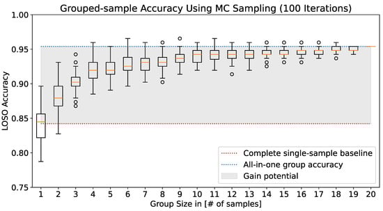
Figure 4. Growth in two-class ($T_0$ vs. $T_4$) LOSO accuracy over grouped predictions per patient, with an increasing number of samples per group. Each box plot visualizes the LOSO accuracy distribution for the respective group size, which is approximated through MC sampling of random groups over 100 iterations. The accuracy gain potential (gray-shaded area) signifies the performance discrepancy between deterministic single-sample classification (red-dotted line) and pain class prediction grouped over all test instances (blue-dotted line).

5. Discussion

5.1. Perspectives on Pain Assessment

Our proposed MM-SCAAE framework opens new perspectives on the reliability of automated pain recognition systems through the integration of multiple biopotentials into the decision-making process, and by proving state-of-the-art performance on multimodal pain recognition using the BioVid dataset. Nevertheless, the current superiority of unimodal models [13,14] with highly specialized network architectures based on the EDA signal points to the major limitation of multimodal approaches, which lies in their proportional scaling to the number of involved sensors. This means that despite the architectural flexibility of MM-SCAAE to subsume unimodal feature extractors, there remains a strict trade-off between model capability and computational requirements.

Regarding the practical realization of pain assessment systems, we believe that multimodal approaches are crucial for trustworthiness and acceptance in health care. Individual sensor contribution may vary, particularly in clinical environments in the real world, as a result of patients’ conditions, medical treatments or external factors. Hence, we propose our MM-SCAAE model for future research attempts to broaden the inclusion of other biopotentials into automated pain assessment. The demonstrated gain in pain recognition accuracy by means of grouped-prediction estimates stemming from multiple samples of length 5.5 s also reveals a potential mismatch between dataset benchmarking based on short-term observations and evaluation for practical applicability. More precisely, we argue that an approximate pain recognition performance of 95% for an extended observation window of around 110 s is still acceptable for the vast majority of clinical applications, since patients would instead need to articulate their subjective pain perception for proper diagnosis. In cases of non-communicative patients (e.g., infants, mentally impaired or unconscious persons), the performance gain established through the grouped-prediction estimate may significantly improve the quality of pain diagnosis. Thus, we are convinced that the collection of real-word datasets with enlarged observation periods is the key to closing the gap between pain research and its practical application.

5.2. Generic Multi-Sensor Pretraining for Time-Series Classification

The pain recognition experiments demonstrated that a key benefit of our pretraining model is that it refrains from comprehensive signal preprocessing in terms of feature engineering (cf. [3,5,9,10,11]) and dimensionality reduction (cf. [6,7,8,12]). In particular, MM-SCAAE directly applies a kind of dimensionality reduction on the raw input signals by means of the introductory MSCNN, which was inspired by the state-of-the-art works [13,14] on unimodal pain recognition. Moreover, our model merely needs half of the pretraining epochs of former methods [6,12,13,14]. These circumstances may serve as indicators for the general capacity of MM-SCAAE.

Apart from the concrete use case of pain recognition, we declare MM-SCAAE as generic model for multi-sensor pretraining which can be tailored by implementing application-specific autoencoder components. Ideally, we would plug in as many sensors as available to maximize the confidence in model predictions, and the model should apply a relevance-weighted information fusion. To make this scenario feasible, MM-SCAAE delivers a rather lightweight architecture which linearly scales with the sensor count. Specifically, the enrichment of AAEs with a SupCon objective also constitutes a generic model type, forming an interesting future research direction.

5.3. Supervised Contrastive Adversarial AutoEncoder (SCAAE)

Adversarial regularization is superior for distribution discrimination compared to the trivial KL-divergence regularizer of VAEs, since adversarial regularization cannot be easily tricked (see Section 2.2.2), and its computational effort is negligible for small two-layer MLPs like we used in the MM-SCAAE framework. During our experiments, we especially did not encounter training instabilities, as is known from the generally error-prone GAN [35] training procedure. As a unique characteristic, the integration of the SupCon objective enhances the primary SAAE [34] framework through class partitioning of latent spaces. For further information about the performance of SCAAE, we refer to Appendix D, where we provide an empirical verification for its effectiveness and generative capabilities. Due to the restricted scope of this paper, we did not explore unsupervised or semi-supervised contrastive AAEs. However, we hypothesize that—even without label information—diverse representation learning algorithms may benefit from auxiliary contrastive regularizations. We hope that future research efforts will evolve the theoretical framework of contrastive AAEs.

5.4. Limitations of This Study and Future Work

The BioVid dataset focuses on short-term measurements of biophysiological pain reactions with a length of 5.5 s. We hypothesize that longer observations of certain modalities could change their individual contribution. In particular, we are convinced that a longer observation of the heart rate for better capturing its variability should facilitate pain classification. Hence, we identify the need for collecting new datasets which account for the latency in the pain reaction of certain modalities. Moreover, we empirically verified the performance of our proposed approach with experiments on the heat pain dataset BioVid, because it is publicly available and its usage is widely spread. However, it could be an interesting future research perspective to investigate the performance of our MM-SCAAE pretraining framework on pain recognition datasets with diverse pain reasons (e.g., electric shock or tactile pressure). Nevertheless, only the gathering of real-world datasets with distinctive pain reasons will eventually allow for the reliable evaluation of state-of-the-art pain recognition models for practical applicability.

Although our model empirically proved resilience against partial sensor failure, our experiments on modality significance emphasized that performance can still dramatically degenerate if highly contributing sensors are unavailable. However, such degeneration effects should constantly reduce with the inclusion of further sensors. Thus, a promising direction for future work is the exploration of other sensors in the clinical setting (e.g., for respiration or blood pressure) to assure trustworthy pain recognition. Our experimental results demonstrated the generalizability of the proposed MM-SCAAE framework in the challenging domain of pain recognition, where datasets are typically scarce and highly biased through the use of small subject groups. In the case of BioVid, for instance, the whole dataset stems from measurements of merely 87 patients. Moreover, we restrict the application scope of the designed MM-SCAAE pretraining model to multimodal time-series classification. Since we strictly focus in our study on the task of pain recognition, we encourage future research efforts that investigate the general capacity of the MM-SCAAE framework and its sensitivity to parameter settings for a wide spectrum of time-series classification tasks. Due to the introduction of an ordinal SupCon loss, it would be especially interesting to exploit inter-class relationships for improving performance in ordinal classification tasks.

The core contribution of our study concerns the technical realization of automated pain recognition systems based on the BioVid heat pain database, which originates from a controlled experiment with healthy probands and standardized environmental factors. We briefly mentioned in our work that in realistic clinical settings patients suffer from diseases, receive medication and may be exposed to external factors, which may drastically change pain-related body reactions. Nevertheless, we did not provide a structural guidance for the hard requirements on pain recognition systems that may arise in a real-world setting. More precisely, our technically oriented study did neither examine the influence of interference factors (e.g., mental conditions, diseases or medication) nor cover the aspect of patient diversity (e.g., ethnic or cultural background) on the resulting performance of pain recognition models. It is necessary to address all these aspects in future research attempts to promote trustworthiness in automated pain recognition. Due to the intrusion of such systems into the subjective perception of individuals, practical applications must ultimately be accompanied with medical ethics and regulatory compliance to prevent the potential misuse of this sensitive information.

6. Conclusions

In this paper, we proposed the multi-sensor pretraining framework MM-SCAAE for addressing the task of multimodal pain recognition based on three selected biophysiological signals. MM-SCAAE combines simultaneous autoencoder training with adversarial and supervised contrastive regularization to ensure robust representation learning. We designed task-specific implementations for all MM-SCAAE components and conducted comprehensive experiments on the BioVid dataset to prove the model’s capability for automated pain recognition. In particular, we achieved a new state-of-the-art in terms of accuracy and $F_1$-score for the multimodal case. Our convincing results should steer researchers’ attention away from unimodal methods and back to multimodal approaches for improving the trustworthiness of pain recognition systems. Finally, we showed that grouped-prediction approaches have the potential to significantly boost the quality of pain assessment in practice.

Appendix D.1. Experimental Setup

To empirically verify the above statements, we conduct experiments on the handwritten digit dataset MNIST [37,38] (version used from TensorFlow Datasets [71]) for a qualitative comparison using an analog model architecture to [34]. Therefore, the encoder and decoder networks consist of two 1000-unit hidden layers with Rectified Linear Unit (ReLU) activation. The encoder ends with a dense layer of two units and linear activation, while the decoder comprises a final 784-unit layer with sigmoid activation. In contrast to [34], our deterministic discriminator network is simplified to a 256-unit hidden layer followed by a 128-unit hidden layer with ReLU activation. The discriminator’s output layer contains a single neuron with sigmoid activation. The fusion network utilizes the same structure as the discriminator but owns 32 output neurons with linear activation. The fusion network normalizes its final outcome using the squash function in Equation (9) (with $\alpha =0.1$) or via unit-vector conversion, depending on the performed experiment. A Batch Normalization [64] layer takes place in each fully connected layer before applying the activation function, except for output layers. The training configuration comprises a 2D Gaussian prior distribution with constant zero mean and standard deviation of 5, the addition of noise $\sim \mathcal{N}(0,0.05)$ to the logits of the discriminator labels, a batch size of 128, a SupCon loss temperature of $\tau =0.1$, the application of an exclusive Adam [66] optimizer with AMSGrad [67] for the generative model and a second one for the discriminator, 100 training epochs, and a constant learning rate of ${10}^{-4}$.

Figure A1. Generalized framework of Supervised Contrastive Adversarial AutoEncoder (SCAAE) trained on MNIST using a 2D Gaussian prior distribution with zero mean and a standard deviation of 5. Visualization of the learned 2D latent encoder space based on MNIST’s hold-out test set for (a,e) nominal and (b,f) ordinal $ϵ$–SupInfoNCE loss. (a,b) conduct squash normalization while (e,f) utilize unit-vector normalization in the last layer of the fusion network. (c,d) display the reconstructions within the feature range of $[-10;10]$ (step size $=2$) for the generative encoder spaces from (a,b), respectively.

Appendix D.2. Nominal ϵ–SupInfoNCE Loss

In the first experiment, the nominal $ϵ$–SupInfoNCE loss in Equation (11) is used where samples from all differing class-to-class pairs are treated equally. Since the fusion network restricts output vectors to magnitudes in the range of $[\alpha ,1]$, we choose the margin parameter

$$ϵ={\displaystyle \frac{1}{n-1}}$$

(A2)

for n classes to obtain a proportional space exploitation. For MNIST with its ten digit classes, this means a desired minimal margin $ϵ\approx 0.1$ between samples from two classes. Figure A1 illustrates the experimental results based on the learned latent encoder space for the squash function in (a) and for the unit-vector normalization in (e). In both cases, SCAAE ensures that the encoder space approaches the 2D Gaussian prior distribution. Specifically, the encoder spaces shape sections within the prior distribution that are clearly separated and exclusively associated with a single digit class. During optimization, the encoder has to make a trade-off between the competitive goals of generative ability and class encapsulation. The decoded latent representations in (c) for the encoding space (a) visualize the learned generative capability with smooth inter-class transitions. In practice, we found that during multiple runs, the squash variant tends to converge faster and to more convincing results, supporting our reasoning in Appendix B. Compared to traditional SAAE [34], our approach needs neither an a priori assignment of dedicated prior distributions to classes nor the direct bypassing of label information to the decoder network. Moreover, the success of bypassing label information has the central disadvantage of being dependent on the number of latent dimensions, i.e., with growing latent dimensionality, class information tends to be stored redundantly, which can harm class separation. Our SCAAE approach eliminates these shortcomings, leading to a more robust SAAE variant.

Appendix D.3. Ordinal ϵ–SupInfoNCE Loss

In the next experiment, the impact of the ordinal $ϵ$–SupInfoNCE loss in Equation (15) on the latent encoder space is investigated by enforcing an artificial class-ordinality constraint on MNIST. In general, we define a circulant graph consisting of the nominal class labels as nodes (i.e., class indices from 0 to $n-1$). If we assume more than six classes, then the circulant class-to-class distance matrix can be described as

$$D_{n>6}=\left[\begin{array}{cccccc}0& 1& 2& \dots & 2& 1\\ 1& 0& 1& 2& \dots & 2\\ 2& 1& 0& 1& & 3\\ ⋮& ⋮& 1& 0& \ddots & ⋮\\ 2& 3& & \ddots & \ddots & 1\\ 1& 2& \dots & 2& 1& 0\end{array}\right].$$

(A3)

As unique characteristic, the circulant matrix repeats per row and column circular versions of the same vector

$${\mathbf{d}}_{n>6}={\left[\begin{array}{ccccccccc}0& 1& 2& \dots & m& \dots & 3& 2& 1\end{array}\right]}^T,$$

(A4)

respectively shifted by row or column index. The value (and index) of the mean element m with the longest distance can be determined with $m={\displaystyle \frac{n}{2}}$, if the condition $nmod2=0$ is true. If n is an odd number then $m={\displaystyle \frac{n-1}{2}}$, and the m value has to be repeated one time before distances start to lower. The ten digit classes from MNIST constitute for the first class (with zero-index) the distance vector

$${\mathbf{d}}_{n=10}={\left[\begin{array}{cccccccccc}0& 1& 2& 3& 4& 5& 4& 3& 2& 1\end{array}\right]}^T.$$

(A5)

According to Equation (14), we formulate the rank-based $ϵ$-margin function between the classes i and j as

$$f_{ϵ}\left(r_{ij}\right)=0.1·{\mathbf{d}}_{n=10}\left(r_{ij}\right),r_{ij}=|i-j|,$$

(A6)

where the coefficient $0.1$ represents the minimal margin between samples from different classes, and ${\mathbf{d}}_{n=10}\left(k\right)$ resolves to the k-th vector element of ${\mathbf{d}}_{n=10}$. Note that the relation ${\mathbf{d}}_{n=10}\left(r_{ij}\right)=D_{n=10}(i,j)$ holds due to the access of vector elements by relative class distance as offset. Figure A1 displays the latent encoder spaces for the squash function in (b) and for the unit-vector normalization in (f). Again, both ordinal loss variants result in a successful approximation of the 2D Gaussian prior distribution, with clearly separated sections assigned to specific classes. In particular, the configuration with the squash function as the normalization strategy perfectly matches the artificially defined circular class-ordinality constraint. This circumstance can be further verified with the respective digit generations in (d), where digits from zero to nine are arranged counter-clockwise with smooth inter-class transformations. The latent encoding space of the unit-vector normalization in (f) reveals a deficit in conserving the predefined class ordinality. We hypothesize that this situation originates from a reduced encoding space exploration during training caused by the unit-vector conversion. Note that we applied both configurations a few runs and selected the best reached results, since the ordinality objective means a soft constraint as part of a multimodal optimization that can not ensure converging to the optimal solution each time. Nevertheless, we observed in total a significantly higher result quality and consistency utilizing the squash function. Thus, SCAAE provides the built-in capability to support ordinality-aligned classification through the definition of task-oriented $ϵ$-margin functions.

References

- Werner, P.; Al-Hamadi, A.; Niese, R.; Walter, S.; Gruss, S.; Traue, H.C. Towards Pain Monitoring: Facial Expression, Head Pose, a new Database, an Automatic System and Remaining Challenges. In Proceedings of the British Machine Vision Conference (BMVC), Bristol, UK, 9–13 September 2013; pp. 1–13. [Google Scholar]
- Walter, S.; Gruss, S.; Ehleiter, H.; Tan, J.; Traue, H.C.; Werner, P.; Al-Hamadi, A.; Crawcour, S.; Andrade, A.O.; Moreira da Silva, G. The BioVid Heat Pain Database: Data for the Advancement and Systematic Validation of an Automated Pain Recognition System. In Proceedings of the 2013 IEEE International Conference on Cybernetics (CYBCO), Lausanne, Switzerland, 13–15 June 2013; pp. 128–131. [Google Scholar] [CrossRef]
- Werner, P.; Al-Hamadi, A.; Niese, R.; Walter, S.; Gruss, S.; Traue, H.C. Automatic Pain Recognition from Video and Biomedical Signals. In Proceedings of the 22nd International Conference on Pattern Recognition (ICPR), Stockholm, Sweden, 24–28 August 2014; pp. 4582–4587. [Google Scholar] [CrossRef]
- Thiam, P.; Kestler, H.A.; Schwenker, F. Two-Stream Attention Network for Pain Recognition from Video Sequences. Sensors 2020, 20, 839. [Google Scholar] [CrossRef] [PubMed]
- Lopez-Martinez, D.; Picard, R. Continuous Pain Intensity Estimation from Autonomic Signals with Recurrent Neural Networks. In Proceedings of the 40th Annual International Conference of the IEEE Engineering in Medicine and Biology Society (EMBC), Honolulu, HI, USA, 18–21 July 2018; pp. 5624–5627. [Google Scholar] [CrossRef]
- Thiam, P.; Bellmann, P.; Kestler, H.A.; Schwenker, F. Exploring Deep Physiological Models for Nociceptive Pain Recognition. Sensors 2019, 19, 4503. [Google Scholar] [CrossRef]
- Thiam, P.; Kestler, H.A.; Schwenker, F. Multimodal Deep Denoising Convolutional Autoencoders for Pain Intensity Classification based on Physiological Signals. In Proceedings of the 9th International Conference on Pattern Recognition Applications and Methods (ICPRAM), Valletta, Malta, 22–24 February 2020; pp. 289–296. [Google Scholar] [CrossRef]
- Gouverneur, P.; Li, F.; Adamczyk, W.M.; Szikszay, T.M.; Luedtke, K.; Grzegorzek, M. Comparison of Feature Extraction Methods for Physiological Signals for Heat-Based Pain Recognition. Sensors 2021, 21, 4838. [Google Scholar] [CrossRef]
- Kächele, M.; Thiam, P.; Amirian, M.; Werner, P.; Walter, S.; Schwenker, F.; Palm, G. Multimodal Data Fusion for Person-Independent, Continuous Estimation of Pain Intensity. In Proceedings of the Engineering Applications of Neural Networks (EANN), Rhodes, Greece, 25–28 September 2015; pp. 275–285. [Google Scholar] [CrossRef]
- Kächele, M.; Amirian, M.; Thiam, P.; Werner, P.; Walter, S.; Palm, G.; Schwenker, F. Adaptive confidence learning for the personalization of pain intensity estimation systems. Evol. Syst. 2017, 8, 71–83. [Google Scholar] [CrossRef]
- Kächele, M.; Thiam, P.; Amirian, M.; Schwenker, F.; Palm, G. Methods for Person-Centered Continuous Pain Intensity Assessment From Bio-Physiological Channels. IEEE J. Sel. Top. Signal Process. 2016, 10, 854–864. [Google Scholar] [CrossRef]
- Thiam, P.; Hihn, H.; Braun, D.A.; Kestler, H.A.; Schwenker, F. Multi-Modal Pain Intensity Assessment Based on Physiological Signals: A Deep Learning Perspective. Front. Physiol. 2021, 12, 720464. [Google Scholar] [CrossRef]
- Lu, Z.; Ozek, B.; Kamarthi, S. Transformer encoder with multiscale deep learning for pain classification using physiological signals. Front. Physiol. 2023, 14, 1294577. [Google Scholar] [CrossRef] [PubMed]
- Li, J.H.; Luo, J.C.; Wang, Y.S.; Jiang, Y.X.; Chen, X.; Quan, Y.J. Automatic Pain Assessment Based on Physiological Signals: Application of Multi-Scale Networks and Cross-Attention. In Proceedings of the 13th International Conference on Bioinformatics and Biomedical Science (ICBBS), Hong Kong, 18–20 October 2024; pp. 113–122. [Google Scholar] [CrossRef]
- Li, G.; Yu, Y. Visual Saliency Detection Based on Multiscale Deep CNN Features. IEEE Trans. Image Process. 2016, 25, 5012–5024. [Google Scholar] [CrossRef] [PubMed]
- Chen, W.; Shi, K. Multi-scale Attention Convolutional Neural Network for time series classification. Neural Netw. 2021, 136, 126–140. [Google Scholar] [CrossRef] [PubMed]
- Zeiler, M.D.; Krishnan, D.; Taylor, G.W.; Fergus, R. Deconvolutional Networks. In Proceedings of the IEEE Computer Society Conference on Computer Vision and Pattern Recognition (CVPR), San Francisco, CA, USA, 13–18 June 2010; pp. 2528–2535. [Google Scholar] [CrossRef]
- Vaswani, A.; Shazeer, N.; Parmar, N.; Uszkoreit, J.; Jones, L.; Gomez, A.N.; Kaiser, L.; Polosukhin, I. Attention Is All You Need. In Proceedings of the 31st Conference on Neural Information Processing Systems (NIPS), Long Beach, CA, USA, 4–9 December 2017; pp. 1–11. [Google Scholar]
- Sabour, S.; Frosst, N.; Hinton, G.E. Dynamic Routing Between Capsules. In Proceedings of the 31st Conference on Neural Information Processing Systems (NIPS), Long Beach, CA, USA, 4–9 December 2017; pp. 3859–3869. [Google Scholar] [CrossRef]
- Kingma, D.P.; Welling, M. Auto-Encoding Variational Bayes. In Proceedings of the International Conference on Learning Representations (ICLR), Banff, AB, Canada, 14–16 April 2014; pp. 1–14. [Google Scholar]
- Rezende, D.J.; Mohamed, S.; Wierstra, D. Stochastic Backpropagation and Approximate Inference in Deep Generative Models. In Proceedings of the 31st International Conference on Machine Learning (ICML), Beijing, China, 21–26 June 2014; Volume 32, pp. 1278–1286. [Google Scholar]
- Hinton, G.E.; Salakhutdinov, R.R. Reducing the Dimensionality of Data with Neural Networks. Science 2006, 313, 504–507. [Google Scholar] [CrossRef] [PubMed]
- Hihn, H.; Gottwald, S.; Braun, D.A. Bounded Rational Decision-Making with Adaptive Neural Network Priors. In Proceedings of the Artificial Neural Networks in Pattern Recognition (ANNPR), Siena, Italy, 19–21 September 2018; pp. 213–225. [Google Scholar] [CrossRef]
- Hihn, H.; Braun, D.A. Specialization in Hierarchical Learning Systems. Neural Process. Lett. 2020, 52, 2319–2352. [Google Scholar] [CrossRef]
- Genewein, T.; Leibfried, F.; Grau-Moya, J.; Braun, D.A. Bounded Rationality, Abstraction, and Hierarchical Decision-Making: An Information-Theoretic Optimality Principle. Front. Robot. AI 2015, 2, 27. [Google Scholar] [CrossRef]
- Hihn, H.; Braun, D.A. Hierarchical Expert Networks for Meta-Learning. In Proceedings of the 4th International Conference on Machine Learning (ICML) Workshop on Life Long Machine Learning, Vienna, Austria, 12–18 July 2020; pp. 1–11. [Google Scholar]
- Ortega, P.A.; Braun, D.A. Thermodynamics as a theory of decision-making with information-processing costs. Proc. R. Soc. A Math. Phys. Eng. Sci. 2013, 469, 20120683. [Google Scholar] [CrossRef]
- Higgins, I.; Matthey, L.; Pal, A.; Burgess, C.; Glorot, X.; Botvinick, M.; Mohamed, S.; Lerchner, A. β-VAE: Learning Basic Visual Concepts with a Constrained Variational Framework. In Proceedings of the 5th International Conference on Learning Representations (ICLR), Toulon, France, 24–26 April 2017; pp. 1–22. [Google Scholar]
- Steur, N.A.K.; Schwenker, F. A Step Towards Neuroplasticity: Capsule Networks with Self-Building Skip Connections. AI 2025, 6, 1. [Google Scholar] [CrossRef]
- Seung, H.S. Learning Continuous Attractors in Recurrent Networks. Adv. Neural Inf. Process. Syst. 1997, 10, 654–660. [Google Scholar]
- Vincent, P.; Larochelle, H.; Bengio, Y.; Manzagol, P.A. Extracting and Composing Robust Features with Denoising Autoencoders. In Proceedings of the 25th International Conference on Machine Learning (ICML), Helsinki, Finland, 5–9 July 2008; pp. 1096–1103. [Google Scholar] [CrossRef]
- Im, D.J.; Ahn, S.; Memisevic, R.; Bengio, Y. Denoising Criterion for Variational Auto-Encoding Framework. In Proceedings of the Thirty-First AAAI Conference on Artificial Intelligence, San Francisco, CA, USA, 4–9 February 2017; Volume 31, pp. 2059–2065. [Google Scholar] [CrossRef]
- Srivastava, N.; Hinton, G.; Krizhevsky, A.; Sutskever, I.; Salakhutdinov, R. Dropout: A Simple Way to Prevent Neural Networks from Overfitting. J. Mach. Learn. Res. 2014, 15, 1929–1958. [Google Scholar]
- Makhzani, A.; Shlens, J.; Jaitly, N.; Goodfellow, I.; Frey, B. Adversarial Autoencoders. In Proceedings of the 4th International Conference on Learning Representations (ICLR), San Juan, Puerto Rico, 2–4 May 2016; pp. 1–16. [Google Scholar] [CrossRef]
- Goodfellow, I.J.; Pouget-Abadie, J.; Mirza, M.; Xu, B.; Warde-Farley, D.; Ozair, S.; Courville, A.; Bengio, Y. Generative Adversarial Nets. Adv. Neural Inf. Process. Syst. 2014, 27, 1–9. [Google Scholar]
- Creswell, A.; Bharath, A.A. Denoising Adversarial Autoencoders. IEEE Trans. Neural Networks Learn. Syst. 2019, 30, 968–984. [Google Scholar] [CrossRef] [PubMed]
- LeCun, Y.; Bottou, L.; Bengio, Y.; Haffner, P. Gradient-Based Learning Applied to Document Recognition. Proc. IEEE 1998, 86, 2278–2324. [Google Scholar] [CrossRef]
- Deng, L. The MNIST Database of Handwritten Digit Images for Machine Learning Research. IEEE Signal Process. Mag. 2012, 29, 141–142. [Google Scholar] [CrossRef]
- Hinton, G.; Sabour, S.; Frosst, N. Matrix Capsules with EM Routing. In Proceedings of the 6th International Conference on Learning Representations (ICLR), Vancouver, BC, Canada, 30 April–3 May 2018; pp. 1–15. [Google Scholar]
- Hinton, G.E.; Krizhevsky, A.; Wang, S.D. Transforming Auto-Encoders. In Proceedings of the 21st International Conference on Artificial Neural Networks (ICANN), Espoo, Finland, 14–17 June 2011; pp. 44–51. [Google Scholar] [CrossRef]
- Steur, N.A.K.; Schwenker, F. Next-Generation Neural Networks: Capsule Networks With Routing-by-Agreement for Text Classification. IEEE Access 2021, 9, 125269–125299. [Google Scholar] [CrossRef]
- Khosla, P.; Teterwak, P.; Wang, C.; Sarna, A.; Tian, Y.; Isola, P.; Maschinot, A.; Liu, C.; Krishnan, D. Supervised Contrastive Learning. Adv. Neural Inf. Process. Syst. 2020, 33, 1–13. [Google Scholar]
- Barbano, C.A.; Dufumier, B.; Tartaglione, E.; Grangetto, M.; Gori, P. Unbiased Supervised Contrastive Learning. In Proceedings of the Eleventh International Conference on Learning Representations (ICLR), Kigali, Rwanda, 1–5 May 2023; pp. 1–24. [Google Scholar]
- Poole, B.; Ozair, S.; van den Oord, A.; Alemi, A.A.; Tucker, G. On Variational Bounds of Mutual Information. In Proceedings of the 36th International Conference on Machine Learning (ICML), Long Beach, CA, USA, 10–15 June 2019; Volume 97, pp. 5171–5180. [Google Scholar]
- Böhm, V.; Seljak, U. Probabilistic Autoencoder. Trans. Mach. Learn. Res. 2022, 1–25. [Google Scholar] [CrossRef]
- Rezende, D.J.; Mohamed, S. Variational Inference with Normalizing Flows. In Proceedings of the 32nd International Conference on Machine Learning (ICML), Lille, France, 6–11 July 2015; pp. 1–10. [Google Scholar]
- Dinh, L.; Sohl-Dickstein, J.; Bengio, S. Density Estimation Using Real NVP. In Proceedings of the 5th International Conference on Learning Representations (ICLR), Toulon, France, 24–26 April 2017; pp. 1–32. [Google Scholar]
- Steur, N.A.K.; Schwenker, F. Class-Variational Learning With Capsule Networks for Deep Entity-Subspace Clustering. IEEE Access 2023, 11, 117368–117384. [Google Scholar] [CrossRef]
- Rezaabad, A.L.; Vishwanath, S. Learning Representations by Maximizing Mutual Information in Variational Autoencoders. In Proceedings of the IEEE International Symposium on Information Theory (ISIT), Los Angeles, CA, USA, 21–26 June 2020; pp. 2729–2734. [Google Scholar] [CrossRef]
- Chapelle, O.; Weston, J.; Bottou, L.; Vapnik, V. Vicinal Risk Minimization. Adv. Neural Inf. Process. Syst. 2000, 13, 1–7. [Google Scholar]
- Tian, Y.; Krishnan, D.; Isola, P. Contrastive Multiview Coding. In Proceedings of the 16th European Conference on Computer Vision (ECCV), Glasgow, UK, 23–28 August 2020; pp. 776–794. [Google Scholar] [CrossRef]
- Liu, Y.; Fan, Q.; Zhang, S.; Dong, H.; Funkhouser, T.; Yi, L. Contrastive Multimodal Fusion with TupleInfoNCE. In Proceedings of the IEEE/CVF International Conference on Computer Vision (ICCV), Montreal, QC, Canada, 10–17 October 2021; pp. 734–743. [Google Scholar] [CrossRef]
- Sermanet, P.; Lynch, C.; Chebotar, Y.; Hsu, J.; Jang, E.; Schaal, S.; Levine, S. Time-Contrastive Networks: Self-Supervised Learning from Video. In Proceedings of the IEEE International Conference on Robotics and Automation (ICRA), Brisbane, QLD, Australia, 21–25 May 2018; pp. 1134–1141. [Google Scholar] [CrossRef]
- Xie, S.; Gu, J.; Guo, D.; Qi, C.R.; Guibas, L.; Litany, O. PointContrast: Unsupervised Pre-training for 3D Point Cloud Understanding. In Proceedings of the 16th European Conference on Computer Vision (ECCV), Glasgow, UK, 23–28 August 2020; pp. 574–591. [Google Scholar] [CrossRef]
- Yang, X.; Zhang, Z.; Cui, R. TimeCLR: A self-supervised contrastive learning framework for univariate time series representation. Knowl.-Based Syst. 2022, 245, 108606. [Google Scholar] [CrossRef]
- Yu, J.; Gao, X.; Zhai, F.; Li, B.; Xue, B.; Fu, S.; Chen, L.; Meng, Z. An adversarial contrastive autoencoder for robust multivariate time series anomaly detection. Expert Syst. Appl. 2024, 245, 123010. [Google Scholar] [CrossRef]
- Mai, S.; Zeng, Y.; Hu, H. Learning from the global view: Supervised contrastive learning of multimodal representation. Inf. Fusion 2023, 100, 101920. [Google Scholar] [CrossRef]
- Ba, J.L.; Kiros, J.R.; Hinton, G.E. Layer Normalization. arXiv 2016, arXiv:1607.06450v1. [Google Scholar] [CrossRef]
- Hendrycks, D.; Gimpel, K. Gaussian Error Linear Units (GELUs). arXiv 2016, arXiv:1606.08415v5. [Google Scholar]
- He, K.; Zhang, X.; Ren, S.; Sun, J. Delving Deep into Rectifiers: Surpassing Human-Level Performance on ImageNet Classification. In Proceedings of the IEEE International Conference on Computer Vision (ICCV), Santiago, Chile, 7–13 December 2015; pp. 1026–1034. [Google Scholar] [CrossRef]
- Python Programming Language. Python Software Foundation: Beaverton, OR, USA. Available online: https://www.python.org/ (accessed on 18 September 2025).
- Chollet, F. Keras. 2015. Available online: https://keras.io (accessed on 18 September 2025).
- Abadi, M.; Agarwal, A.; Barham, P.; Brevdo, E.; Chen, Z.; Citro, C.; Corrado, G.S.; Davis, A.; Dean, J.; Devin, M.; et al. TensorFlow: Large-Scale Machine Learning on Heterogeneous Distributed Systems. arXiv 2015, arXiv:1603.04467v2. [Google Scholar]
- Ioffe, S.; Szegedy, C. Batch Normalization: Accelerating Deep Network Training by Reducing Internal Covariate Shift. In Proceedings of the 32nd International Conference on Machine Learning (ICML), Lille, France, 6–11 July 2015; pp. 448–456. [Google Scholar]
- Loshchilov, I.; Hutter, F. Decoupled Weight Decay Regularization. In Proceedings of the Seventh International Conference on Learning Representations (ICLR), New Orleans, LA, USA, 6–9 May 2019; pp. 1–11. [Google Scholar]
- Kingma, D.P.; Lei Ba, J. Adam: A Method for Stochastic Optimization. In Proceedings of the 3rd International Conference on Learning Representations (ICLR), San Diego, CA, USA, 7–9 May 2015; pp. 1–15. [Google Scholar] [CrossRef]
- Reddi, S.J.; Kale, S.; Kumar, S. On the Convergence of Adam and Beyond. In Proceedings of the Sixth International Conference on Learning Representations (ICLR), Vancouver, BC, Canada, 30 April–3 May 2018; pp. 1–9. [Google Scholar]
- Szegedy, C.; Vanhoucke, V.; Ioffe, S.; Shlens, J.; Wojna, Z. Rethinking the Inception Architecture for Computer Vision. In Proceedings of the IEEE Conference on Computer Vision and Pattern Recognition (CVPR), Las Vegas, NV, USA, 27–30 June 2016; pp. 2818–2826. [Google Scholar] [CrossRef]
- Fragoso, T.M.; Bertoli, W.; Louzada, F. Bayesian Model Averaging: A Systematic Review and Conceptual Classification. Int. Stat. Rev. 2018, 86, 1–28. [Google Scholar] [CrossRef]
- Hoeting, J.A.; Madigan, D.; Raftery, A.E.; Volinsky, C.T. Bayesian Model Averaging: A Tutorial. Stat. Sci. 1999, 14, 382–417. [Google Scholar] [CrossRef]
- TensorFlow Datasets: A Collection of Ready-to-Use Datasets. Available online: https://www.tensorflow.org/datasets (accessed on 12 March 2025).
Disclaimer/Publisher’s Note: The statements, opinions and data contained in all publications are solely those of the individual author(s) and contributor(s) and not of MDPI and/or the editor(s). MDPI and/or the editor(s) disclaim responsibility for any injury to people or property resulting from any ideas, methods, instructions or products referred to in the content. |
© 2025 by the authors. Licensee MDPI, Basel, Switzerland. This article is an open access article distributed under the terms and conditions of the Creative Commons Attribution (CC BY) license (https://creativecommons.org/licenses/by/4.0/).