Abstract
Ballistic impact mitigation requires the development of protective armor applications from composite material systems with good energy absorption and penetration resistance against threats, e.g., metallic projectiles. In this aim, high-strength and high-stiffness soft fibrous composite materials (such as ultra-high molecular weight polyethylene—UHMWPE) are often used. The high specific strength feature is one of the main reasons for using these soft composite systems in ballistic impact applications. In the present investigation, experimental and computational finite element (FE) studies were carried out to investigate the ballistic behaviors of these soft layered composite targets. To this end, a new FE multi-scale analysis framework for ballistic simulations is offered. The proposed analysis presents a new meso-scale sublaminate material model, which is applied to Dyneema® cross-ply laminate in order to predict its behavior under ballistic impact. The sublaminate model is implemented within an explicit dynamic FE code to simulate the continuum response in each element. The sublaminate model assumes a through-thickness periodic stacking of repeated cross-ply configuration. In addition, a cohesive layer is introduced in the sublaminate model in order to simulate the delamination effect leading to the subsequent degradation and deletion of the elements. This new approach eliminates the widely used costly computational approach of using explicit cohesive elements installed at pre-specified potential delamination paths between the layers. Furthermore, in-plane damage modes (such as fiber tensile, and out-of-plane shearing) are also accounted for by employing failure criteria and strain-softening. The obtained quantitative results of ballistic impact simulations show good correlation when compared to a relatively wide range of experiments. Moreover, the simulations include evidence of capturing the main energy absorption mechanisms under high-velocity impact. The proposed modeling approach can be used as a useful armor design tool.
1. Introduction
High costs and the limited amount of data from ballistic experiments have led researchers to develop numerical models for predicting the performance of fabric armor systems under ballistic impact. Moreover, the predictive capability of the numerical method in such cases is used to guide armor designers and to upgrade the basic understanding of the mechanics of ballistic penetration beyond the current analytical methods and experimental capabilities. These models have been the subject of interest for many years in the defense and commercial industries. However, due to the complexity involved in describing the response of fabric armor, most models attempt to provide the most acceptable trade-off in performance analysis. The complicated composition leads to several failure mechanisms. These can be attributed to constituents having different properties and many layer orientations, which make the modeling of such composites more complicated, compared to heavy steel armor.
This complexity of the problem has forced researchers [1,2] to accept certain simplifying assumptions to make the problem more tractable. Thus, Iannucci and Pope [2] presented a model, which is based on Cunniff’s [3] dimensionless equations for ballistic impact systems. Their model uses shell elements without delamination between the layers. Comparison between the model results in real impact tests demonstrating the challenge to represent all the failure mechanisms, but it showed qualitatively similar deformation and the same response as the impact tests. The success of the model was based on setting the correct properties of the tensile, compressive and shear response of the material. Sharma et al. [4] developed a finite difference model of an ultra-high molecular weight polyethylene (UHMWPE) composite plate, Dyneema UD66 HB1, under ballistic impact and compared it to ballistic range experiments. Their model does not present the micromechanical failure mechanisms, since it was simple and two-dimensional. However, the main failure mechanisms at the macro level were shown, and good agreement with the experimentally measured velocity was presented. A numerical model for the material’s V50 prediction was developed by Heisserer and Van der Werff [5]. The material was modeled by representative continuum elements, with strong in-plane orthotropic properties. Each directions’ failure criterion was calibrated to adjust one of the low ultrasonic velocity measurements that determined the parameters of the linear elastic stiffness matrix. A parametric study of the strength, density and inputted modulus was carried out and the predictions of the model agreed well with the experiments. The results showed a reduction in the ballistic performance with higher modulus, while higher strength enhances it.
One of the greatest challenges in the understanding of a composite material armor system under ballistic impact leans on characterizing the energy absorption mechanisms it possesses. Mines et al. [6] identified three modes of energy absorption when analyzing the ballistic perforation of composites with different shapes of projectile: local perforation, delamination and friction between the projectile and the target. They also identified three through-thickness regimes in terms of local perforation, namely: I—shear failure, II—tensile failure and III—tensile failure and delamination. Delamination can propagate under Mode I (opening) and Mode II (shear) loading. Out of these three regimes, the through-thickness perforation failure is dominated by shear failure (observed by [7], as well). Three energy absorption mechanisms were quantified and considered by Morye et al. [8] in response to the polymeric composite system: kinetic energy of the formed bulge, tensile failure of primary yarns and the elastic deformation of secondary yarns. A comparison was made between the high-speed photography data and the numerical results. For most of the tested materials, a good correlation was shown, but not for the Dyneema. It can be assumed that one of the reasons is neglecting delamination—the main failure mechanism of Dyneema [9,10,11]. The numerical model of Harel and Marom [12] was based on the energy absorption summation of cross-ply plates such as PE (Polyethylene)/PE [0/90] by two mechanisms: delamination energy and fiber breakage energy. The total energy was compared to the measured kinetic energy of the bullets. It found that the delamination energy was much more dominant compared to the energy of fiber breakage. Another work with a similar conclusion was carried out by Cunniff [3]. Two energy absorptions of an armor system were numerically modeled: fiber breakage—strain energy due to fiber axial elongation, and kinetic energy—resulting from transverse velocity of the system. A good match was received between the model’s predictions and the experimental results. It was found that when the projectile’s velocity was much higher than the critical striking velocity, energy absorption such as fiber breakage is negligible.
Parametric investigation allows one to not only calibrate the numerical model against analytical and experimental results, but also rapidly study the effect of many factors such as material properties [13], geometry, friction, and projectile characteristics on the impact performance. To determine the system effects of single-ply and then fabric plies in body armor systems, Cunniff [14] compared the reaction of spaced armor systems to actual multiple-ply systems. He noted that the energy absorption characteristics of body armor systems under ballistic impact depend on material parameters (constitutive properties and material failure criteria), construction parameters (system areal density, fabric type and number of fabric plies) and impact conditions (geometry, projectile mass and striking velocity). The work of Naik et al. [15] considers parameters such as perforation and the partial penetration of the projectile into the target [16], cone (bulge) formation on the exit side of the target [7,17], effect of stress wave transmission factor, thickness of the target [10,17] and the mass and diameter of the projectile [10]. Other parameters such as ballistic limit [10,16,17,18], contact duration at the ballistic limit [10] and residual velocity [10,18], were studied in function of the different target and projectile parameters. The parameters which were predicted and compared with those from an experiment in Lim et al.’s [19] investigation were the ballistic limit, residual velocity, energy absorption and transverse deflection profiles of the fabric.
Similar to Lim et al.’s work, Ramadhan et al. [20] performed a numerical parametric study to predict the energy absorbed by the target, ballistic limit velocity and comparison between experimental and simulation work.
In the present article, a model is offered based on the sublaminate model [21], which was mainly developed for thick-section composite laminate. Despite the fact that thick-section composites, nearly up to failure, may show almost linear overall structural behavior, nonlinear response can emerge too (the presence of structural discontinuities and edge effects, such as holes, tips and cutouts). For this reason, it was important to develop an analysis method—the sublaminate model, for this kind of composites, which includes both 3D and nonlinear capabilities. There are three main advantages of the model:
First, its ability to modify the tensile and shear modulus, in-plane tension and shear on each step in the analysis (see Section 2.1.2).
The model allows to simulate the local delamination damage throughout itself, in order to degraded the out of plane (OP) properties (so-called distributed delamination, see Section 2.4.1), by weakening the material’s effective properties without actually inserting a gap where the cohesive layer is placed.
The method for implementing the three dominant failure modes with the Tsai–Wu failure criteria into the sublaminate model is shown in Section 2.4.3.
The current study aimed to perform a parametric study on this new computational model of high-velocity impact simulations, representing the Dyneema composite system; Then, the model was validated and calibrated against experimental data and results from ballistic tests.
This article is organized as follows. Section 2 represents the material system, followed by presenting the experimental procedure and its results. In addition, this section represents the proposed model—the sublaminate model, its implemented failure criteria and the finite element (FE) structural implementation. To the end, Section 3 represents the results and discussion, followed by concluding the achievements of this study (Section 4).
2. Materials and Methods
2.1. Material System
Dyneema from DSM is a brand name for an UHMWPE fiber-reinforced composite. This soft polymeric material system is assembled from four alternating unidirectional (UD) orthotropic laminae in two fibers orientations, one in the 0° direction and the second in 90° direction, forming the [0/90/0/90] laminate in a polyurethane resin. The Dyneema’s density is about 970 kg/m3 and its fiber volume content is high and up to the geometric limit, which is about 83% [22]. The targets in the experiments are made of Dyneema HB26 (HB stands for Hard Ballistics). Its areal density is between 0.257 and 0.271 kg/m2 [23]. It is manufactured by the gel spinning process for producing its fibers, progress to ply fabrication towards thermo-pressing at high temperature and pressure to final laminate production according to the manufacturer’s (DSM) recommendation (the exact temperature and pressure are proprietary of Plasan Sasa Ltd.). Its fiber (SK76) tensile strength and modulus values are 3.6 and 120 GPa, respectively, with an elongation at failure of 3.8% [24].
2.1.1. Mechanical Properties of Dyneema HB26
The mechanical properties of the 0° ply direction at Dyneema HB26 layer are obtained based on the microstructure of a representative volume element (RVE, see Section 2.3.2), the volume fraction of the fiber and matrix, and their respective properties [25] (see Table 1).

Table 1.
Dyneema HB26 orthotropic layer properties, adapted from [25] E11, E22, E33 are the Young’s modulus in each of the three axes; G12, G13, G23 are the Shear modulus in each plane; and ν12, ν13, ν23 are the Poisson ratio in each plane.
2.1.2. Non-Linear Stress–Strain Relation in Tension and Shear
Since the polymeric composites, e.g., Dyneema, behave in a non-linear manner with respect to loading, a stress–strain relation was defined to behave accordingly. In-plane tension and shear experiments were conducted on laminated specimens of Dyneema HB26 to account for the non-linear tensile and shear modulus [26]. The non-linear relation is defined as follows:
where K and m are constants, which are calibrated according to the experimental curves. and are the tensile modulus and the strain of a single UD layer ([0] or [90]) of the sublaminate, respectively. The only variable on this relation is the strain, and it is important to note that after softening, the tensile modulus cannot increase again, which ensures that the material does not regain stiffness after being deformed. The values used for the curve fitting are: , .
The shear modulus was modified by fitting the Ramberg–Osgood (RO) [27] in relation to the measured experimental stress–strain curves [26], as follows:
where , and are constants which determine the shape of the curve, and the only variable that changes accordingly by the shear modulus
, is the shear stress . Similarly to the previous relation, it is important to note that after softening, the shear modulus cannot increase again (it ensures that the material does not regain stiffness after being deformed). The values used for the curve fitting are: , = 3, , .
2.2. Experimental Procedure and Results
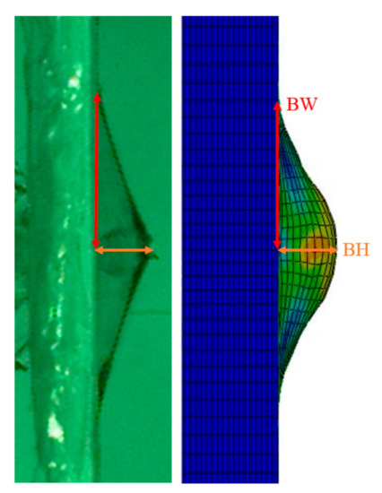
To obtain the ballistic performance of Dyneema HB26, a series of ballistic tests were conducted in Plasan’s shooting range laboratory. The composite target plates, with dimensions of 400 × 400 mm2, were firmly clamped on their edges. These composite targets were impacted on their center point by fragment simulating projectile (FSP) 2.85 gr (44 grain, MIL-P-46593) projectiles at varying velocities. A high-speed camera was used to record the impact events, one frame on each 27 µs, producing a side view of the projectile penetration process on the targets. This visual data were used to extract the basic test parameters for each impact test, such as the residual velocity (Vr), the bulge height (BH) and the bulge width (BW), which will be used for calibration with the FEM simulations. The shooting data and the results from the experiments are shown in Table 2.
Table 2.
Experimental shooting data on the Dyneema HB26 composite target.
2.3. Method of Analyses (The Proposed Model)
There is a great amount of research on the Dyneema’s behavior under various loading cases. The challenge of the designers is to try to fit the failure and energy absorption mechanisms, assuming they are correct, to an appropriate computational representation of the material. Then, the ballistic impact of different threats upon this material target is simulated on FE software. The ballistic impact experiments are very expensive, and the simulations offer a needed alternative. Presently, there is a collision between the model’s precision and its cost-efficiency. If the model is too simplified (macro-scale model), it will run faster, but has the potential risk of giving the wrong conclusions about the material system’s ability to protect against threats, which can obviously lead to devastating outcomes. On the other hand, a detailed model (micro-scale model) which calculates all the target’s energy absorption mechanisms with each time increment, can easily cost even more than the experimental procedures and thus cannot be considered as an expedient replacement. Therefore, a reasonable compromise is required.
2.3.1. The Sublaminate Model
The suggested model employed in this study is the sublaminate model. It is generated from the smallest through-thickness repeating stacking sequence (see Figure 1) of the laminae, and its effective response is used to describe the equivalent nonlinear homogeneous continuum. As a result, the effective homogeneous 3D continuum behavior of the material points is generated by the sublaminate model at each integration point in the FE structural mesh. This model accounts for the material’s micro-scale structure as an input for the properties of the orthotropic layers used in the meso-scale. The meso-scale is the middle scale between the micro and macro levels, which is a compromise between two of those scales’ shortcomings (and answers to the earlier request for a reasonable compromise). This fact means that this model cannot represent micro-level failure modes, such as matrix cracking and fiber-matrix de-bonding. Nevertheless, it is believed to be accountable for the main energy absorption mechanisms detected in the mechanical characterization study—fiber tensile failure, delamination and out-of-plane shearing. The focus on these three main mechanisms also shortens the calculations, by making the model more efficient. One more consideration that supports these assumptions relies on the fact that under extremely high rate loads (order of magnitude around 105/s) and a very short loading period (µs) of the impact, these modes of failure are highly dominant, while the others are local and do not take place widely at these loading conditions. In other words, it seems that under ballistic impact, the cohesion between adjacent layers will fail before the failure of the bond between the fiber and matrix. In addition, the transverse impact on a fiber-reinforced material will cause extensive tension in the fibers, in an endeavor to stop the projectile from penetrating through the plate, while fiber kinking and matrix cracking are more likely to occur under long-term and local loads.
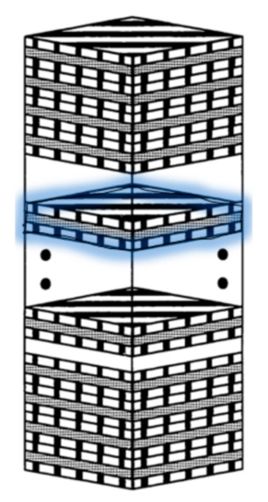
Figure 1.
Example of the repeating stacking sequence (bolded in light blue), which the sublaminate is using to describe an equivalent nonlinear homogeneous continuum.
The sublaminate model and its equations, which are presented in the next sections, are implemented to Abaqus/Explicit through a Fortran VUMAT subroutine. The effective properties of a sublaminate, representing properties at an integration point of the 3D element in Abaqus. Therefore, the VUMAT’s equations are the link between the sublaminate model and Abaqus/Explicit.
2.3.2. The Model’s Structure
The structure of a representative sublaminate’s volume element, composed of a [0] layer and a [90] layer (perpendicular to each other), with an interfacial cohesive layer (see Figure 2). The axes of the layer are defined as: 1—the direction of the fibers; 2—direction normal to the fiber orientation; whereas the 3 direction is the out-of-plane direction. Each layer of the laminate is labeled by a serial upper indices, k = 1, 2,…, n, where n is the number of layers in a laminate. In the sublaminate model, k = 1, 2, and 3 denote the [0], [90] and the cohesive layers, respectively (see Figure 2). The cohesive layer is considered as infinitely thin, used as an interface between the orthotropic layers. It has large out-of-plane strength and small in-plane strength in order to perform the traction–separation relation of the orthotropic layers leading to delamination.
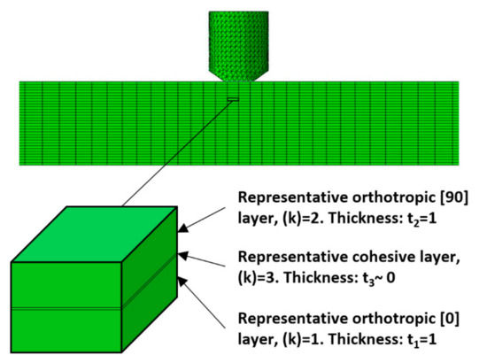
Figure 2.
Representative volume element (RVE) of the sublaminate model.
2.3.3. The Sublaminate Mathematical Formulation
This section presents the main feature formulation of the nonlinear sublaminate model, using the 3D lamination theory for finding the mechanical effective stress–strain relations and the effective stiffness of the sublaminate.
The strain–stress relation of an elastic material is given by
where —strain tensor; —compliance matrix of the material; —stress tensor. Equation (3) can be written explicitly:
The values of the parameters in the compliance matrix are given in Table 1. In order to use the unique features of the sublaminate, a set of simple algebraic manipulations are performed. Equation (4) leads to the following:
The sub-matrices , , and are 3 × 3 and contain the appropriate components of the original compliance matrix, relating the in- and out-of-plane strains to the stresses. The indices i and o represent the in-plane (IP) and out-of-plane (OP) components of the strain vectors:
and the stress vectors:
The in-plane components refer to the 1–2 plane of the laminate, the same plane on which the [0] and [90] orthotropic layers are laid upon and possess high tensile properties. The OP direction (3 plane) is normal to these layers (1–2 plane) and controls the interfacial strength between the layers.
Each layer has a local orientation coordinate system rotated with respect to the global one. Therefore, when referring to a specific layer’s stress and strain components, it is necessary to distinguish between a local layer’s components, which apply along its orthotropic axes, and the same components in global terms. In our case, [0] layer has θ = 0° and the [90] has θ = 90°. Transforming a local tensor to the global coordinate system is performed with a transformation matrix, and a bar notation appears above the transformed tensor of the kth layer, as follows:
where is the strain transformation matrix and is the stress transformation matrix.
Perfect Bonding Conditions
As long as the composite laminate is undamaged, the layers are perfectly bonded. This leads to two following conditions, accountable for perfect bonding:
This homogeneous in-plane global strain and homogeneous out-of-plane global stress are used to satisfy the conditions of displacement and the traction continuity between the layers. This means that when a laminated composite is deformed in-plane, all layers stick together and undergo equal straining, , (Equation (10)). It also verifies that if out-of-plane stress is applied to the material, all layers ‘feel’ the same stress , and remain perfectly attached to each other (Equation (11)). In other words, if the first condition does not hold, one of the layers slips with respect to the other, indicating a failure of the adhesion between them. If the second condition does not hold, a gap appears between the adjacent layers and prevents the stresses from being transferred between them, implying that there is a delamination initiation in their interface:
Partial Inversion—The ABD Matrix
With a few other algebraic manipulations, referred to as partial inversion, Equation (5) can be written for each layer as
where the components of the ABD matrix are defined as ; ; and = ;
The local relation (Equation (12)) can be rewritten in global terms, after using the coordinate transformation, as
After using the perfect bonding conditions on the last relation, it leads to:
Effective Sublaminate Properties
According to Equation (14), the effective sublaminate properties (indicated by astric) can then be calculated as follows:
where is the number of the layers and , , and represent the thicknesses of layers 1–3. In this model: ( is the cohesive layer) and (unit thickness).
The effective compliance matrix of the sublaminate, , can be obtained by using the method of partial inversion and the global effective ABD matrix. The effective stiffness matrix, , which is the inverse matrix of effective compliance matrix (), can be obtained as well:
Finally, the global stress state of the sublaminate can be obtained by using the effective stiffness matrix as a function of the strain state. As already mentioned and shown in this section, the effective properties of the sublaminate, representing an integration point of the material’s continuum, are derived from the relative part of each of the layer’s properties. This demonstrates the behavior of a composite laminate as a function of its constituents and meso-scale structure.
2.4. The Model’s Failure Criteria
One of the important capabilities of the presented model is that it can be employed as a basis for implementing various failure criteria. The model lays the foundations for a hierarchical multi-scale structure of the material. This implies that smaller-scale failure modes (like micro-cracks, fiber-matrix de-bonding, etc.) can be implemented in the model if further refinements of each layer are performed (such as using micromechanics to model a unit cell of fiber and matrix). On the one hand, it will probably raise the accuracy, but on the other hand, it will complicate the model and will increase the calculation time, resulting in a less attractive feature.
2.4.1. Distributed Delamination
The first failure criterion used in the model is related to the OP stress state in the cohesive layer. Once this criterion is fulfilled, the degradation of out-of-plane properties is applied. This allows the model to simulate local delamination damage or distributed delamination. The criterion given in the following equation uses Equation (14) with k = 3 (the cohesive layer):
The above criterion is activates only the degradation of the sublaminate’s effective properties. This makes the failed element’s zone less resistant to out-of-plane stresses, which are imposed extensively in transverse ballistic impact. This fact is one of the strengths of the model, since the failed zone gives an expression for the delamination’s effect on the weakening of the material’s effective properties (so-called distributed delamination) without actually inserting a gap where the cohesive layer is placed.
2.4.2. Tsai–Wu Failure Criterion for Anisotropic Materials
The model uses the general form of the Tsai–Wu failure criterion [28] as follows:
where ; ; ; ; ; ; ; ; and are the ultimate stresses in tension and compression, in-plane of a laminate, respectively. and are the ultimate stresses in tension and compression, out-of-plane, respectively. and are the ultimate shear stresses, in and out of plane, respectively.
The normal and shear stresses on a single element of the composite material are shown in Figure 3. The Tsai–Wu failure criterion considers the total strain energy for predicting failure when the failure index in an orthotropic laminate reaches unity. Some of the reasons for using this failure criterion in this study, stems from the fact that it fits better than the other failure criteria to experimental data, and it is reliable and easy to use in computational procedures.
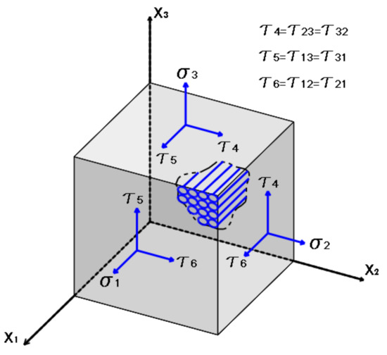
Figure 3.
Normal and shear stresses on a single element of the composite material.
The Tsai–Wu polynomial is applied on a single integration material point in the element in order to detect failure initiation. This procedure is applied on the entire sublaminate elements.
Determining the strengths of the material in different loading modes can be achieved by performing experiments at high rates for the specific modes of failure. This implies a large experimental program, which is difficult to perform, to monitor and to extract the needed data. Thus, insufficient dynamic experiments are currently available to contribute to a meaningful database. The method chosen here for that matter is to use rough estimations of the ultimate stresses, based on the knowledge about their nature and the experimental procedures [26] described above. Then, through simulations, to modify the parameters to obtain a result as close to reality as possible. This calibration is performed according to certain parameters, which will be explained later. The explanations behind the assumptions and the values of the ultimate stresses, are described in Mustacchi work [25]. The assumptions are as follows:
- •
- •
- •
where is the rate of the IP degradation factor and is the RO is the softening initiation stress.
The assumptions that were described above contribute to decreasing the running time of the model. Therefore, some of the model’s parameters were reduced in order to decrease the number of possible parameter combinations. These were implemented in VUMAT to reduce the running time for convergence of the model to a reasonable one (several hours). The model’s seven strength parameters and four RO fit parameters are presented in Table 3.
Table 3.
The model’s 7 strength parameters and 4 Ramberg–Osgood (RO) fit parameters.
2.4.3. Implementation of the Tsai–Wu Failure Criteria on the Sublaminate Model
In order to determine the main failure modes in the impacted composite target, our study had to distinguish between cases when the ultimate value of (see Equation (18)) leads to failure and when it does not. Then, to develop a set of failure modes typical to the materials under ballistic impact. The method monitors the components of the Tsai–Wu polynomial (TW[#]), in order to check which term dominates the failure of elements at every point across the plate’s section. Each component of the polynomial is inserted into an array as shown in Table 4.
Table 4.
Implementation of the Tsai–Wu failure criteria into the sublaminate model.
The stress state at each point is expressed by the Tsai–Wu polynomial and the components of the TW array are compared in order to find the maximal one and store its index in a user’s state variable (SDV). The stored data are an indication of the dominating stresses active at a point and indicate which failure modes are more likely to occur. The correct utilization of the data can be used for a fairly accurate model of the energy absorption distribution over an impacted plate. The results obtained from the SDV’s array, pointed to the following three dominant failure modes.
- Delamination—It has been identified as a leading energy absorption mechanism of the Dyneema composite, especially under ballistic impacts. After inspecting the data presented by the SDV, the delamination failure term (local failure—for element’s elimination) is:The first term in Equation (19) accounts for a total failure according to the Tsai–Wu polynomial. The second term accounts for the failure only under the condition of positive ultimate normal stresses, as these tend to separate the adjacent layers.
- Fiber tension—a major energy absorption mechanism is included in the tensile straining of fibers. In addition to the fact that composites possess high tensile energy absorbing capabilities, fibers that suffer high tensile straining directly under the impacting projectile tend to tear. The local tensile failure term (for element’s elimination) is:If the values of and are greater than for both UD layers, local tensile failure has been achieved and the element is eliminated.
- First incident shear tearing—high OP pressure inflicted on the first impacted layers by the projectile, tear these layers and allow the projectile to penetrate through the plate, thus keeping the damage localized. This mode occurs in the first stage of the projectile’s impact when it possesses high kinetic energy causing early element deletion.The relevant term for this failure mode is defined byThis mode of failure requires a combination of local Tsai–Wu ultimate state and ultimate OP shear stresses, or .
2.5. FE Structural Implementation
This section describes the ballistic impact simulations, which were carried out with Abaqus/Explicit, using a VUMAT user’s subroutine, written in Fortran source code. The details of the model, such as material model definition, the typical loads, boundary conditions, element type and meshing are presented in the next section.
2.5.1. Ballistic Impact Simulation
The purpose of the proposed finite-element analysis (FEA) is to simulate the ballistic impact tests carried out by Plasan for matching the format, which was carried out at the shooting laboratory. The model (see Figure 4) simulates a user-defined material (Dyneema) plate with dimensions of 400 × 400 mm2. Both the composite and projectile were modeled in full geometry to be able to simulate the stress waves propagating in the composite plate target starting from the impact point towards the clamped edges and back. This will exhibit how the composite will respond. The thicknesses of the Dyneema Plates are 8.7 mm. The model also includes a FSP 2.85 gr projectile with steel material properties, modeled as a rigid body (no deformation—an assumption verified by experimental visual data and previous studies, such as [2,8,29,30,31]).
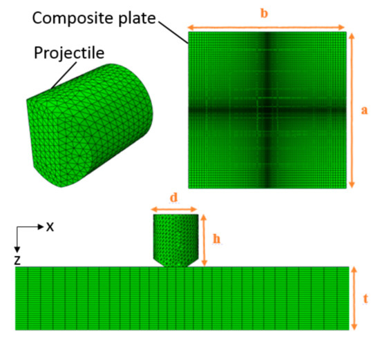
Figure 4.
Mesh and dimensions of the composite plate and the projectile.
The plate was discretized by 432,000 solid hexahedral elements of type C3D8R, which are linear, three-dimensional and have reduced integration (contain eight nodes and one integration point) elements, with 30 elements through the thickness. An important feature for the success of the model is the use of a bias parameter towards the middle of the plate’s in-plane mesh. This bias parameter decreases the size of the elements, by approaching the impact point, where deformations and stresses are more dominant than in the plate’s periphery. Furthermore, the projectile was meshed by 10,923 non-reduced solid tetrahedral elements of type C3D4 (containing four nodes) which are also linear and three-dimensional elements. The projectile is chosen as isotropic material with a Young’s modulus of 205 GPa, Poisson ratio of 0.3 and density of 7830 kg/m3.
Similar to the experimental setup, the plate was clamped (fixed) at its four ends and subjected to impact by the projectile with an initial velocity (Vinitial) in the Z direction (see Figure 4).
Finally, a general contact is defined, such as all element surfaces are allowed to contact with each other. This type of contact is crucial since the elimination of elements caused by failure leads to new potential interactions and continuous deformation between adjacent layers and between the projectile to the layers. The plate’s and projectile’s materials, dimensions, DOF (degrees of freedom), boundary conditions, number of elements and their type are described in Table 5.
Table 5.
Summary of the FEA model’s data.
The analysis is performed over a time period of 100 μs, with automatic incrementation of 5 μs intervals.
A mesh sensitivity study was conducted in order to check how it affects post-failure and simulation results. Three different mesh densities were used over the plate, and the results have shown a mesh-dependency and that the calibrated parameters are valid for a small range of the mesh length scale. This phenomenon is common in softening and energy dissipation due to damage, especially in highly dynamic and ballistic impact simulations. The latter is also valid due to the high strain rates and sizeable inelastic deformation, leading to the degradation and failure by localized damage and fracture [11]. In addition, the element removal due to material failure and excessive deformation process enhances strain softening and adds to mesh size dependency. Nonlocal constitutive damage formulation is needed to alleviate this phenomenon, e.g., [32,33,34].
2.5.2. Success Parameter of the Model
The many DOFs and numerous possible combinations of analysis simulations results create a need for an overall success parameter (SP) to account for the relative weight of each of the studied measurements. This parameter will indicate a close enough evaluation of the model’s performance under different sets of the critical values used in the simulation.
This study used four main parameters for comparison to determine the success of the model, as follows:
These four parameters were chosen since they defined the ability of an armor system to absorb the energy of the threat, in order to prevent it from being transferred to the protected subject. These parameters may pose measurement errors, which are difficult to overcome, and should be taken into account while estimating the total performance of the model. Considering this fact, relative weights were given to the SP of the model, as follows:
where , and are the residual velocity, bulge height and bulge width relative errors, respectively.
An example of one component of the relative error:
The residual velocity of the projectile is in direct relation with the damage, which is inflicted on the target. It is also the most important measure and the easiest to determine from the current data sets, and thus is given the highest weight (50%). The second important parameter is the bulge height (30%), since it is closely related to the potential of harming a person behind it. If the projectile is stopped, we would like to know how deep the bulge is as a measure of the probability of injury. Moreover, it is easier to measure than the bulge’s width, which is the least important parameter (20%). This third parameter is the least harmful feature of the overall material response and has the most errors in measurement. This model’s SP calculation approach seems to capture all the previous approaches reviewed in other studies [4,8,35,36,37] and forms a step forward for improving the evaluation quality of the ballistic impact model.
3. Results and Discussion
This section presents the experimental and computational results obtained from four main sub-sections: (Section 3.1) parametric study; (Section 3.2) predictions of the calibrated model; (Section 3.3) post-impact comparison; and (Section 3.4) SP calculation.
3.1. Parametric Study
As mentioned, one of the objectives of this study was to perform a parametric study of high-velocity impact simulations on the Dyneema composite material, using the sublaminate model. The parametric investigation was based on changing the values of Xt and Yc for establishing the optimal parameters to be used in the model.
3.1.1. Parametric Study: Changing Xt
The first parametric investigation is based on changing the values of Xt. The chosen values are: Xt = 1, 1.2, 1.4 and 1.6 GPa. All the other strength parameters are kept as given in Table 3. Five of the eight impact velocities: 606, 698, 708, 814 and 893 m/s, were calibrated, but for simplicity, only results for arrest case (606 m/s, see Figure 6), and the perforation case (708 m/s, see Figure 7) are described here. As indicated in Table 2, these results are shown at time 25 µs and 60 µs for the perforation and the arrest case, respectively.
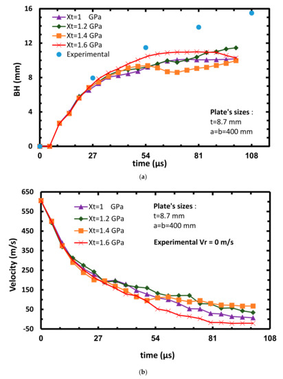
Figure 6.
Plate’s bulge height (a) and projectile’s velocity (b) vs. time at varying Xt, Vinitial = 606 m/s.
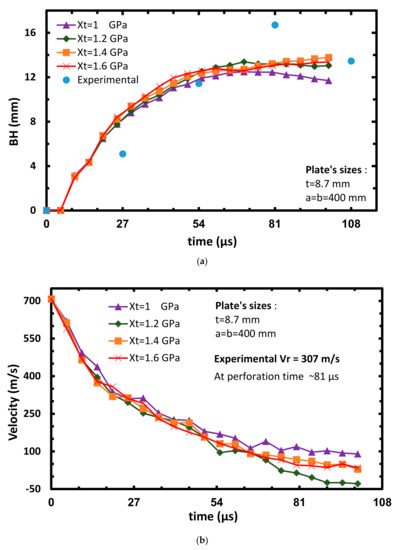
Figure 7.
Plate’s bulge height (a) and projectile’s velocity (b) vs. time at varying Xt, Vinitial = 708 m/s.
The deformation at the center back of the plate (BH) is given by the displacement–time curves (see Figure 6a and Figure 7a). The shape of the curves of these graphs, describes the loss of the projectile’s kinetic energy, which is absorbed by the target vs. time. The curves represent the displacement of one node on the center back face of the plate along the X axis at varying Xt. As can be seen from Figure 6a, after the impact takes place (0–55 µs), most of the plate’s displacement (~10 mm) occurs and it is close to the displacement obtained from the experiment (~11 mm). After that and until the arrest of the projectile, a slight increase in displacement is observed. Figure 7a shows a good correlation between the analysis and the experimental BH, and its value is around 11 mm.
The graph of the velocity vs. time gives the history of the projectile’s velocity (see Figure 6b and Figure 7b). The curves in these graphs represent the average velocity of four random selected nodes, located near the central axis of the projectile at varying Xt. It is important to note that the missing experimental curve of the projectile’s velocity is attributed to the fact that the projectile is hidden from the high-speed camera while it penetrates the target. Therefore, the reported experimental residual velocity is only shown for the perforation cases. Figure 6b shows that the velocity reduces almost linearly soon after the impact takes place. It can be clearly seen that within 70 to 80 µs after the impact, the graph shows a plateau which indicates that the velocity is slightly constant at this range, moving toward the arrest of the projectile (similar to experiments). A rebound effect (negative velocity of the projectile) can be observed for the Xt = 1.6 GPa simulated case towards the arrest of the projectile. The elastic rebound of the bulge can be attributed to the release of strain energy stored in the secondary yarns which convert into the kinetic energy of the projectile [15]. The highest SP value (SP = 84.2) in all the cases is found for the Xt = 1 GPa. An advantage of the model is reflected by the repeatability of the curves on the graphs, meaning that small changes in the model’s parameters cause small changes in the model’s results.
3.1.2. Parametric Study: Changing Yc
The second parametric investigation is based on calibrating the values of Yc. The selected values are: Yc = 1.4, 1.6, 1.8, 2, 2.2, 2.4 and 2.6 GPa, together with Xt = 1 GPa. All the other strength parameters given in Table 3 are kept constant. Here too, two impact velocities’ results are discussed: 606 m/s for the arrest case (see Figure 8) and 708 m/s for the perforation case of the projectile (see Figure 9). Similarly to the previous sub-section, Figure 8a and Figure 9a also show that most of the plate’s displacement (~10 mm) occurs after the impact takes place (0–55 µs) which is close to the measured displacement (~11 mm). Moreover, Figure 9a shows a good correlation between the analysis and the experimental BH as its value is around 11 mm. Figure 8b shows that the velocity exhibits sharp reduction soon after the impact takes place (0–20 µs). This indicates the good energy absorption ability of the Dyneema. Similarly to the experiment, the projectile did not manage to perforate the target in all cases, and stops after 80–90 µs. Figure 9b shows that residual velocity (Vr) is around 100 m/s (note that if Yc = 2.2 GPa is assumed, the resulting Vr is around 220 m/s) while in the experiment, Vr equals to 307 m/s. The linear behavior exhibited after 45 µs of the Yc = 2.2 GPa curve, may be explained by a detached node from the center back face of the model, which travels at a constant speed. After calculating the SP (see Section 3.4) in all the considered cases, it was found that SP = 89.5, which results from Xt = 1 GPa and Yc = 2.2 GPa, and can be considered as the calibrated case.
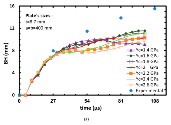
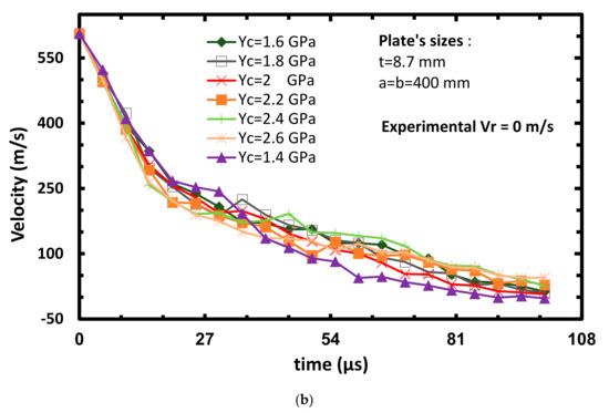
Figure 8.
Plate’s bulge height (a) and projectile’s velocity (b) vs. time at varying Yc, Vinitial = 606 m/s.
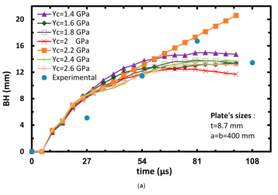
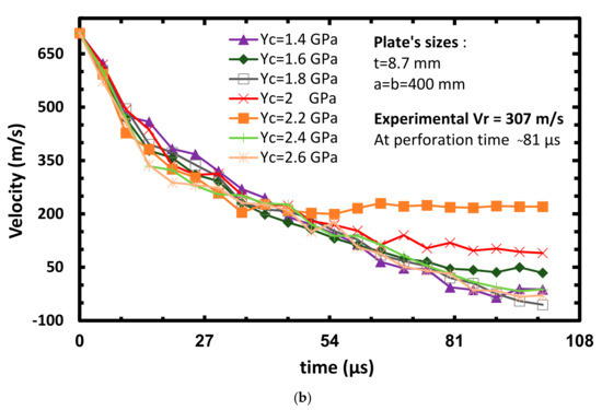
Figure 9.
Plate’s bulge height (a) and projectile’s velocity (b) vs. time at varying Yc, Vinitial = 708 m/s.
Once again, it can be seen that the model is robust, since small changes in the model’s parameters cause small changes in the model’s results and preserve the tendency of the curves.
Another way to show the calibrated model’s strength parameters with Xt = 1 GPa and Yc = 2.2 GPa coupling is by exhibiting the residual velocity vs. initial (impact) velocity graph, (see Figure 10). As can be seen, the closest slope to the experimental one is due to the coupling of Xt = 1 GPa and Yc = 2.2 GPa, as found earlier. Note that the time steps of the high-speed photography and the simulation are not perfectly synchronized, which is caused by the difficulty of catching the exact moment of the impact on the camera between the projectile and plate. Additionally, there are different time steps between the simulation and experiments (5 and 27 µs, respectively).
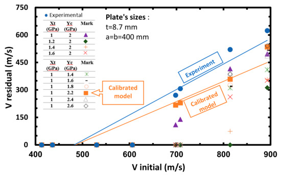
Figure 10.
Projectile’s residual velocity vs. initial velocity at varying Xt and Yc.
To get a first look on the model’s performance against the experiments, an impact process of the projectile with a velocity of 606 and 893 m/s in sequential time steps, is shown in Figure 11 and Figure 12, respectively. The simulation snapshots are the sub-section of the plate’s center along the Y–Z plane. As the projectile hits the target, a bulge is formed as a result of the plate’s transverse impact load, pushing the layers out of the plane. It can be observed that there is a larger bulge in the arrest case (Figure 11) in comparison to the perforation case (Figure 12), since more energy is transferred to deform the target. The existence of the longitudinal stress waves are also evident in both cases, as the material dissipates energy along its fibers away from the impact point. Fiber breakage can be seen in the first stages (0–25 µs) of the simulation, while delamination can be observed at a later time sequence (55–80 µs). Once the projectile perforates the plate, the residual or exit velocity remain constant, since there is no resistance from the plate.
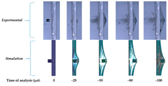
Figure 11.
Sequential time steps after the ballistic impact, Vinitial = 606 m/s.
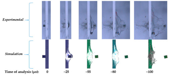
Figure 12.
Sequential time steps after the ballistic impact, Vinitial = 893 m/s.
3.2. Predictions of the Calibrated Model
After performing the parametric investigation and establishing the calibrated model’s strength parameters, the predictions of the calibrated model are presently shown at eight BH vs. time. Figure 13, Figure 14, Figure 15 and Figure 16 present the plates BH vs. time for projectile impact velocities of 413, 436, 530 m/s (as already mentioned, these three cases were not calibrated) and 606 m/s, respectively (arrested cases). Figure 17, Figure 18, Figure 19 and Figure 20 on the other hand present the plates BH vs. time at projectiles impact velocities of 698, 708, 814 and 893 m/s, respectively (perforated cases).
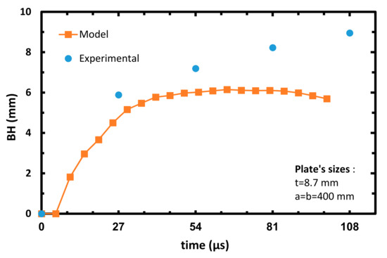
Figure 13.
Plate’s bulge height vs. time of the calibrated model, Vinitial = 413 m/s.
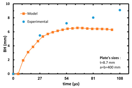
Figure 14.
Plate’s bulge height vs. time of the calibrated model, Vinitial = 436 m/s.
Figure 15.
Plate’s bulge height vs. time of the calibrated model, Vinitial = 530 m/s.
Figure 16.
Plate’s bulge height vs. time of the calibrated model, Vinitial = 606 m/s.
Figure 17.
Plate’s bulge height vs. time of the calibrated model, Vinitial = 698 m/s.
Figure 18.
Plate’s bulge height vs. time of the calibrated model, Vinitial = 708 m/s.
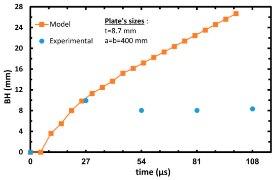
Figure 19.
Plate’s bulge height vs. the time of the calibrated model, Vinitial = 814 m/s.
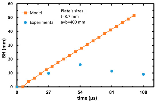
Figure 20.
Plate’s bulge height vs. time of the calibrated model, Vinitial = 893 m/s.
As can be seen from the arrested cases, the model’s prediction in each case is slightly lower than the experimental results. As mentioned above, this can be explained by the fact that most of the energy during the impact in the model’s analysis is invested in delamination. This fact decreases the projectile kinetic energy, which leads to minor BH as compared to the experimental data. Although Figure 17 and Figure 18 represent perforation cases, the projectile managed to perforate the target only at ~81 µs, giving enough time to ‘transfer’ the projectile kinetic energy to delamination of the target. These graphs represent a reversal tendency, since the BH of the model analysis in Figure 18 and Figure 19 are slightly higher than the experimental results. It can be referred to as the decrease in energy transferred to the delamination mode, since more energy is absorbed on fiber breakage due to the contact between the projectile and the target. The almost linear curves starting from 27–54 µs in Figure 18, Figure 19 and Figure 20 can be attributed to the constant velocity of the detached center node of the model (during the perforation of the projectile in the target). From the results of the experiments and the analysis, it can be estimated that ballistic limit- V50 is around 650 m/s.
3.3. Post-Impact Comparison
It is interesting to compare the shape prediction of the calibrated model’s impacted plate with the experimental result. (Figure 21a,b), shows the final shape of the plate as obtained from the experiment and the analysis predictions, respectively. This figure exhibits the resulting delamination, fiber tension and first incident shear tearing delamination damage (marked as 1, 2 and 3, respectively). It can be readily observed that good correspondence by the two approaches exists. It is worth mentioning that the plate was photographed a while after the impact. Therefore, relaxation and other disturbances have ’blurred’ the full magnitude of the deformation patterns, but their essence is still visible. The yellow marking was performed to highlight the three main failure modes.
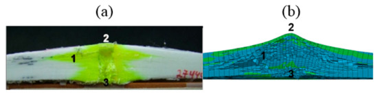
Figure 21.
Plate section post-impact comparison ((a)—experiment; (b)—analysis).
A post-impact section (scale 1:8) of a Dyneema plate by a projectile with an impact velocity of 606 m/s. The main deformation mechanisms are marked: 1—delamination, 2—fiber tension, 3—OP shearing.
3.4. Success Parameter Calculation
Using visual outputs from the Abaqus simulation and high-speed photography, the four success parameters (SP) can be determined. The results of the simulation with comparison to the respective experiments are presented in Table 6 (Vr comparison) and Table 7 (BH and BW comparison). As explained, the ballistic impact event between the composite target and the projectile could end by the arrest or perforation of the projectile as discussed in the following.
Table 6.
Calibrated case’s ballistic simulation results (Vr) compared to the experimental results.
Table 7.
Calibrated case’s ballistic simulation results (BH, BW) compared to the experimental results.
Projectile arrested—partial penetration of the projectile, which starts by hitting the target to the point its velocity becomes zero. This is represented as “No” in the “Perforated” column in Table 6.
Projectile Perforated—complete perforation of the projectile, which starts by hitting the target to the point it exits from the back face of the target. This is represented as “Yes” in “Perforated” column in Table 6.
As can be seen from Table 6, all the projectiles which were supposed to be stopped were stopped, and all the ones which were perforated in the experiments were so in the simulations. The simulation patterns imitate well the ones observed in the experiments. As already reported, the overall SP was calculated and found to be around 89.5% (see Table 7), which is very high.
4. Conclusions
A new multi-scale model for predicting the ballistic impact response of polymeric-fiber laminated composites was presented and applied. The model incorporates the sublaminate mesoscale analysis, which was successfully implemented through a user’s subroutine for the impact FE simulations. The general form of the Tsai–Wu failure criterion was implemented in the subroutine and the Dyneema’s dominant energy absorption and failure mechanisms under the ballistic impact of the projectile were observed and characterized.
A parametric study of high-velocity impact simulations was performed for the Dyneema composite system. The model was validated, and its failure parameters were calibrated against experimental data and results from the laboratory’s ballistic tests. Very good predicted correlation had been obtained. The pre-calibrated multi-scale model was successful in predicting both stopped as well as perforated experiments. Moreover, a good correlation is demonstrated between the experiments and simulations’ Vr (residual velocity), BH (bulge height), and BW (bulge width). The overall SP (success parameter) was calculated and found to be around 89.5%.
One significant achievement of the presented model is its ability to simulate the delamination initiation and growth at an arbitrary location, without using cohesive elements. This reduces the computation time significantly, from days to a few hours, making the models attractive enough to be used for armor design and as a substitute for expensive experimental procedures.
Author Contributions
Conceptualization, R.C. and R.H.-A.; formal analysis, R.C., S.M., E.M. and R.E.; investigation, R.C., S.M., E.M., R.E., J.A. and R.H.-A.; methodology, R.H.-A., R.C., J.A.; project administration, R.H.-A., R.E.; software, R.C., S.M., and E.M.; supervision, R.H.-A.; validation, R.C., S.M. and E.M.; visualization, R.C. and S.M.; writing—original draft, R.C. and S.M.; writing—review and editing, R.C., J.A. and R.H.-A. All authors have read and agreed to the published version of the manuscript.
Funding
Plasan Inc. supported this research and the Israel Science Foundation (ISF) (grant No. 2314/19).
Institutional Review Board Statement
Not applicable.
Informed Consent Statement
Not applicable.
Acknowledgments
This research was supported by the Israel Science Foundation (ISF) (grant No. 2314/19) to the last author. The additional support of the Nathan Cummings Chair of Mechanics is gratefully acknowledged.
Conflicts of Interest
The authors declare no conflict of interest.
References
- Dhandapani, K. Experimental Investigation and Development of a Constitutive Model for Ultra High Molecular Weight Polyethylene Materials. Ph.D. Thesis, Arizona State University, Tempe, AZ, USA, 2009. [Google Scholar]
- Iannucci, L.; Pope, D. High velocity impact and armour design. Express Polym. Lett. 2011, 5, 262–272. [Google Scholar] [CrossRef]
- Cunniff, P.M. A Semiempirical Model for the Ballistic Impact Performance of Textile-Based Personnel Armor. Text. Res. J. 1996, 66, 45–58. [Google Scholar] [CrossRef]
- Sharma, N.; Carr, D.; Kelly, P.; Viney, C. Modelling and Experimental Investigation into the Ballistic Behaviour of an Ultra High Molecular Weight Polyethylene/Thermoplastic Rubber Matrix Composite. In Proceedings of the 12th International Conference on Composite Materials (ICCM-12), Paris, France, 1 July 1999; p. 1. [Google Scholar]
- Heisserer, U.; Van der Werff, H. The relation between Dyneema® fiber properties and ballistic protection performance of its fiber composites. In Proceedings of the 15th International Conference on Deformation, Yield and Fracture of Polymers, Kerkrade, The Netherlands, 1–5 April 2012; Volume 3, pp. 242–246. [Google Scholar]
- Mines, R.A.W.; Gibson, A.G. High velocity perforation behaviour of polymer composite laminates. Int. J. Impact Eng. 1998, 21, 855–879. [Google Scholar] [CrossRef]
- Ćwik, T.K.; Iannucci, L.; Curtis, P.; Pope, D. Investigation of the ballistic performance of ultra high molecular weight polyethylene composite panels. Compos. Struct. 2016, 149, 197–212. [Google Scholar] [CrossRef]
- Morye, S.S.; Hine, P.J.; Duckett, R.A.; Carr, D.J.; Ward, I.M. Modelling of the energy absorption by polymer composites upon ballistic impact. Compos. Sci. Technol. 2000, 60, 2631–2642. [Google Scholar] [CrossRef]
- Meshi, I.; Amarilio, I.; Benes, D.; Haj-Ali, R. Delamination behavior of UHMWPE soft layered composites. Compos. Part B Eng. 2016, 98, 166–175. [Google Scholar] [CrossRef]
- Langston, T. An analytical model for the ballistic performance of ultra-high molecular weight polyethylene composites. Compos. Struct. 2017, 179, 245–257. [Google Scholar] [CrossRef]
- Hazzard, M.K.; Trask, R.S.; Heisserer, U.; Van Der Kamp, M.; Hallett, S.R. Finite element modelling of Dyneema® composites: From quasi-static rates to ballistic impact. Compos. Part A Appl. Sci. Manuf. 2018, 115, 31–45. [Google Scholar] [CrossRef]
- Harel, H.; Marom, G.; Kenig, S. Delamination controlled ballistic resistance of polyethylene/polyethylene composite materials. Appl. Compos. Mater. 2002, 9, 33–42. [Google Scholar] [CrossRef]
- Yuan, Z.; Chen, X.; Zeng, H.; Wang, K.; Qiu, J. Identification of the elastic constant values for numerical simulation of high velocity impact on dyneema® woven fabrics using orthogonal experiments. Compos. Struct. 2018, 204, 178–191. [Google Scholar] [CrossRef]
- Cunniff, P.M. An Analysis of the System Effects in Woven Fabrics under Ballistic Impact. Text. Res. J. 1992, 62, 495–509. [Google Scholar] [CrossRef]
- Naik, N.K.; Shrirao, P.; Reddy, B.C.K. Ballistic impact behaviour of woven fabric composites: Parametric studies. Int. J. Impact Eng. 2006, 32, 1521–1552. [Google Scholar] [CrossRef]
- O’Masta, M.R.; Crayton, D.H.; Deshpande, V.S.; Wadley, H.N.G. Mechanisms of penetration in polyethylene reinforced cross-ply laminates. Int. J. Impact Eng. 2015, 86, 249–264. [Google Scholar] [CrossRef]
- Zhang, T.G.; Satapathy, S.S.; Vargas-Gonzalez, L.R.; Walsh, S.M. Ballistic impact response of Ultra-High-Molecular-Weight Polyethylene (UHMWPE). Compos. Struct. 2015, 133, 191–201. [Google Scholar] [CrossRef]
- Nguyen, L.H.; Lässig, T.R.; Ryan, S.; Riedel, W.; Mouritz, A.P.; Orifici, A.C. Numerical modelling of ultra-high molecular weight polyethylene composite under impact loading. Procedia Eng. 2015, 103, 436–443. [Google Scholar] [CrossRef]
- Lim, C.T.; Shim, V.P.W.; Ng, Y.H. Finite-element modeling of the ballistic impact of fabric armor. Int. J. Impact Eng. 2003, 28, 13–31. [Google Scholar] [CrossRef]
- Ramadhan, A.A.; Abu Talib, A.R.; Mohd Rafie, A.S.; Zahari, R. High velocity impact response of Kevlar-29/epoxy and 6061-T6 aluminum laminated panels. Mater. Des. 2013, 43, 307–321. [Google Scholar] [CrossRef]
- Haj-Ali, R. The Sublaminate Model. In Multiscale Modeling and Simulation of Composite Materials and Structures; Young, W., Kwon, D.H., Allen, R.T., Eds.; Springer: Berlin/Heidelberg, Germany, 2008; pp. 334–341. ISBN 9780387363189. [Google Scholar]
- Russell, B.P.; Kandan, K.; Deshpande, V.S.; Fleck, N.A. The high strain rate response of UHMWPE: From fibre to laminate. Int. J. Impact Eng. 2013, 60, 1–9. [Google Scholar] [CrossRef]
- Royal DSM N.V, DSM—Product Specification Sheet HB26; Royal DSM: Heerlen, The Netherlands, 2011.
- Afshari, M.; Sikkema, D.J.; Lee, K.; Bogle, M. High performance fibers based on rigid and flexible polymers. Polym. Rev. 2008, 48, 230–274. [Google Scholar] [CrossRef]
- Mustacchi, S. Multi-Scale Dynamic Modeling of Projectile Penetration in Soft Polymeric-Fiber Laminated Composite; Tel Aviv University: Tel Aviv, Israel, 2013. [Google Scholar]
- Levi-Sasson, A.; Meshi, I.; Mustacchi, S.; Amarilio, I.; Benes, D.; Favorsky, V.; Eliasy, R.; Aboudi, J.; Haj-Ali, R. Experimental determination of linear and nonlinear mechanical properties of laminated soft composite material system. Compos. Part B Eng. 2014, 57, 96–104. [Google Scholar] [CrossRef]
- Ramberg, W.; Osgood, W.R. Description of Stress-Strain Curves by Three Parameters; Technical Note No. 902; National Advisory Committee for Aeronautics: Washington, DC, USA, 1943. [Google Scholar]
- Tsai, S.W.; Wu, E.M. A General Theory of Strength for Anisotropic Materials. J. Compos. Mater. 1971, 5, 58–80. [Google Scholar] [CrossRef]
- Utomo, D.H. High-speed Impact Modelling and Testing of Dyneema Composite; TUDelft: Delft, The Netherland, 2011; ISBN 9789461910233. [Google Scholar]
- Yong, M.; Iannucci, L.; Falzon, B.G. Efficient modelling and optimisation of hybrid multilayered plates subject to ballistic impact. Int. J. Impact Eng. 2010, 37, 605–624. [Google Scholar] [CrossRef]
- Flanagan, M.P.; Zikry, M.A.; Wall, J.W.; El-Shiekh, A. An Experimental Investigation of High Velocity Impact and Penetration Failure Modes in Textile Composites. J. Compos. Mater. 1999, 33, 1080–1103. [Google Scholar] [CrossRef]
- Abu Al-Rub, R.K.; Kim, S.M. Predicting mesh-independent ballistic limits for heterogeneous targets by a nonlocal damage computational framework. Compos. Part B Eng. 2009, 40, 495–510. [Google Scholar] [CrossRef]
- Park, M.; Yoo, J.; Chung, D.T. An optimization of a multi-layered plate under ballistic impact. Int. J. Solids Struct. 2005, 42, 123–137. [Google Scholar] [CrossRef]
- Krishnan, K.; Sockalingam, S.; Bansal, S.; Rajan, S.D. Composites: Part B Numerical simulation of ceramic composite armor subjected to ballistic impact. Compos. Part B 2010, 41, 583–593. [Google Scholar] [CrossRef]
- Naik, N.K.; Shrirao, P. Composite structures under ballistic impact. Compos. Struct. 2004, 66, 579–590. [Google Scholar] [CrossRef]
- Zhang, Z.; Shen, S.; Song, H.; Zhang, D. Ballistic penetration of Dyneema fiber laminate. Mater. Sci. Technol. 1997, 14, 265. [Google Scholar]
- Hayhurst, C.J.; Leahy, J.; van der Jagt-Deutekom, M.; Jacobs, M.; Kelly, P. Development of Material Models for Numerical Simulation of Ballistic Impact onto Polyethylene Fibrous Armour. In Proceedings of the Personal Armour Systems Symposium 2000 (PASS2000), Colchester, UK, 5–8 September 2000; pp. 169–178. [Google Scholar]
Publisher’s Note: MDPI stays neutral with regard to jurisdictional claims in published maps and institutional affiliations. |
© 2021 by the authors. Licensee MDPI, Basel, Switzerland. This article is an open access article distributed under the terms and conditions of the Creative Commons Attribution (CC BY) license (http://creativecommons.org/licenses/by/4.0/).