Abstract
The influence of hot-top designs with different heat capacities on the distribution of positive and negative macrosegregation was investigated on a 12 metric tonne (MT) cast ingot made using Cr-Mo low-alloy steel. The three-dimensional finite element modeling code THERCAST® was used to simulate the thermo-mechanical phenomena associated with the solidification process, running from filling the mold until complete solidification. The model was validated on an industrial-scale ingot and then utilized to evaluate the influence of the thermal history of the hot-top, a crucial component in the cast ingot setup. This assessment aimed to comprehend changes in solidification time, temperature, and heat flux—all of which contribute to the determination of macrosegregation severity. The results showed that preheating the hot-top had a minor effect on solidification time, while modifications of thermal conductivity in the hot-top region increased the solidification time by 31%, thereby significantly affecting the macrosegregation patterns. The results are discussed and interpreted in terms of the fundamental mechanisms governing the kinetics of solidification and macrosegregation phenomena.
1. Introduction
Ingot casting, followed by forging, is the only route available for the production of large-size components made of specialty steels, such as mill rolls, turbine rotors, power plant shafts, and metal forming dies [1,2]. The composition of these steels is characterized by a large number, often up to 10, of alloying elements. These provide the required mechanical and corrosion resistance properties. During the solidification process of the ingot, heat is removed from the mold, and because of the different diffusion coefficients of the different elements, micro and macrosegregation occurs. While microsegregation indicates the presence of alloying elements above the nominal composition at the interface of dendrite arms, macrosegregation instead corresponds to the heterogeneous distribution of alloying elements over distances of several centimeters in width and up to meters in length. This quality deteriorates the mechanical properties of the final products as it cannot be removed, even after long homogenization heat treatment. The complex interactions and coupling between alloying elements, casting mold characteristics (e.g., mold and hottop geometries, insulations, etc.), and casting parameters (e.g., pouring temperature, rate, etc.) result in very complex interactions. Laboratory-scale experiments are often not representative of the industrial reality, and empirical industrial-scale testing is extremely costly and time-consuming. Therefore, numerical approaches are needed to address these intricate physical phenomena that arise throughout the casting process, allowing for a faster optimization of the casting conditions as well as the quantification of the interactions between and mutual influences of the different parameters [3,4,5,6,7,8,9,10].
Among the various components of the cast ingot setup, the hot-top is identified as the most important one [4]. However, other components such as the mold, refractory material, runner, and trumpet also impact the solidification of the ingot. Specifically, the mold’s geometry affects heat transfer rates, cooling, and flow dynamics during casting, while the design of the runner system influences the molten metal flow, mold filling uniformity, and temperature distribution, all of which ultimately shape the ingot’s properties. As its name indicates, the hot-top is located on the top part of the mold. Its external structure is made of the same material as the ingot mold (i.e., cast iron), and its interior walls are lined with refractory bricks, called sideboard. The top surface of the hot-top is covered by two exothermic caps, which are made of Al, SiO2, and Al2O3 compounds that produce a large amount of heat once the surface of exothermic caps comes into contact with the molten metal. The main exothermic reaction, as dictated by the chemical composition of the exothermic cap, can be described by a specific chemical equation (2Al + Fe2O3 = 2Fe + Al2O3 + Q) [11,12]. The hot-top plays a crucial role in the solidification process and consequently influences the macrosegregation sensitivity of the ingot because it provides the heat flow at the top of the ingot and continuously feeds the ingot with liquid metal as it solidifies. Thus, controlling the heat exchange and thermal regime of the hot-top is of critical importance in decreasing solidification defects like macrosegregation [4,13,14].
The initial research into the design of hot-tops was conducted in a pioneering study by Flemings, who proposed guidelines for achieving the minimum sufficient volume required for feeding the ingot, determined a downward temperature gradient from the hot-top to the ingot body that must be reached, etc. [15,16,17]. Tashiro et al. [14] experimentally and numerically studied the hot-top design condition in 100 MT and 135 MT ingots in a Ni-Cr-Mo-V steel product. They proposed that the hot-top and mold geometry play crucial roles in producing large, high-quality ingots. They reported that the thermal conditions of the hot-top had a lesser impact than the geometrical parameters (the ratio of the hot-top diameter to the ingot diameter and the ratio of the height of the ingot body to the average diameter of the body) on the time and rate of ingot solidification. They reported that the segregation type of “A” can occur when the solidification rate falls below 0.8 mm/min within the internal zone of Ni-Cr-Mo-V steel ingots containing 0.25% C. However, the impact of the hot-top thermal regime on positive and negative segregation, heat transfer, and temperature in the ingot was not reported in their work. The effects of the hot-top insulation condition in a 6.2 MT steel ingot with a nominal carbon concentration of 1.01 (wt.%) were experimentally studied by Kumar et al. [18]. They reported that using exothermic insulation material results in a chemical reaction, which raises the nuclei number. This impacts the microstructure, macrosegregation, and heat exchange in the mold, in the ingot adjacent to the refractory material, and below the hot-top zone. They produced finer axial globular grain structures and observed a more significant axial macrosegregation compared to the case where no exothermic insulation material was used in the hot-top interior walls. However, the influence of using different scenarios to modify the hot-top thermal regime on macrosegregation was not investigated. In addition, the impact of the hot-top thermal regime on heat transfer and temperature in the entire ingot was not quantified. Kermanpur et al. [19] studied the influence of the shape and height of hot-top insulation and slender ratio (height/average diameter of the ingot body) on solidification behavior in a Cr-Mo low carbon steel 6 MT; however, they did not discuss the impact of hot-top characteristics on the extent and severity of macrosegregation. The present investigation, on the other hand, quantitatively explores how the thermal regime of the hot-top influences different elements, such as the extent and severity of macrosegregation, solidification time, temperature evolution, and heat exchange across the entire large ingot body. Specifically, four different scenarios of hot-top heat capacity are investigated. The case study is a 12 MT bottom-poured ingot of high-strength steel used in energy and transportation systems that require very high levels of microstructure homogeneity. The developed FEM model was first experimentally validated on an industrial-size ingot [4] and then used to evaluate the impact of the four investigated thermal regime scenarios.
2. Materials and Methods
Medium carbon low-alloy steel, the composition of which is provided in Table 1, was bottom-poured into a 12 MT capacity polygonal shape mold. The molten metal was produced in an electric arc furnace, after which the molten metal was cleaned using ladle furnace processing and vacuum degassing. Thereafter, the molten metal was poured at 1580 °C from the bottom into the cast iron mold for 26 min. Figure 1a,b show the cast ingot components and hot-top dimensions. The upper part of the hot-top sidewalls was lined with refractory material and the top surface of the hot-top was covered by two exothermic caps.

Table 1.
Nominal chemical composition of studied steel (wt.%).
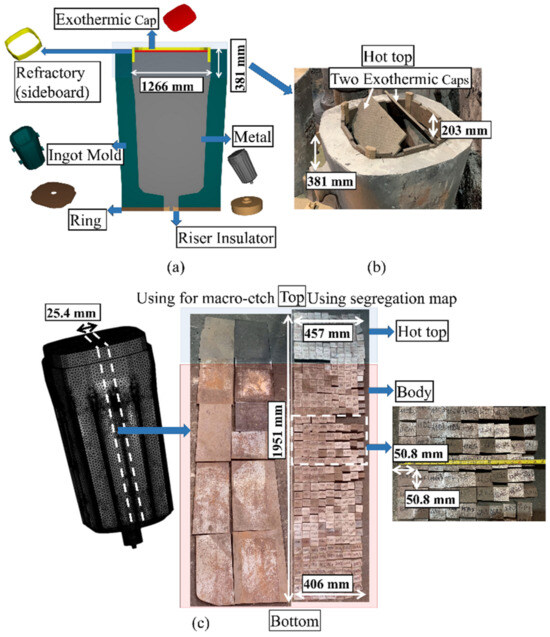
Figure 1.
(a) The cast ingot setup of 12 MT ingot (180° model); (b) hot-top part in industry; and (c) the sample preparation approach.
After completing solidification and cooling to room temperature, a 25.4 mm thick slice of the ingot was cut from the center in the longitudinal direction, as indicated in Figure 1c. The slice was then cut along its length. Then, one of the half-slices was cut into 370 specimens that were used for chemical mapping. The other one was cut into 10 plates that were used for macroetching. Figure 1c schematically shows the approach used for sample cutting and preparation. Chemical analysis of the samples was conducted using a Thermo Scientific ARLTM 4460 Optical Emission Spectrometer (Thermo Fisher Scientific Inc., Waltham, MA, USA), and then the segregation ratios of each sample were calculated using the following equation: Ri = (wi − w0i)/w0i [4,13,20,21]. Here, Ri is the segregation ratio of solute element i, wi is the solute local concentration, and w0i is its initial concentration. A positive or negative Ri value represents positive or negative segregation, respectively. Then, macrosegregation patterns of elements on the total part of the longitudinal section were built using MATLAB® version 2012 (The MathWorks Inc., Natick, MA, USA) [22]. The surfaces of the other 10 plates were etched using a 50% HCl–50% H2O solution at 50 °C to reveal the patterns of macrosegregation [4].
This experimental study was conducted to gain insights into the intensity and evolution of segregation for all alloying elements. It is also important to note that microstructural analysis was not the focus of the present work, but that it was previously performed by our research group and the results were published [21]. In this study, macrosegregation modeling of the 12 MT ingot was simulated using the finite element code (FEM), THERCAST®. The established model was validated via a comparison of the predicted and experimental results of the chemical distribution patterns of alloying elements. The details regarding the validation of the FEM model were presented in a recent publication by the present authors [4]. The validation data are reported in Table A1 and Table A2 and Figure A1 and Figure A2 of Appendix A.
3. Solidification Model Formulation
Three-dimensional FEM simulation of the solidification process was conducted using the finite element code, THERCAST®. Thermo-mechanical phenomena associated with the various phases of mold filling and the process of cooling in and out of the mold were described using an arbitrary Lagrangian–Eulerian (ALE) formulation based on the volume-average two-phase model [23,24]. The fluid flow, temperature, and distribution of solute in the solidifying material were analyzed using the coupled solutions of equations denoting the conservation of mass, momentum, energy, and solute, as indicated in Table 2. Heat transfer equations were solved for each subdomain (mold, hot-top, ingot, sideboard, etc.) using appropriate boundary conditions, including the average convection, radiation, external imposed temperature, and external imposed heat flux. A Fourier-type equation was used for the evaluation of contact resistance at the interfaces of metal and mold components. The convection and radiation equations are also reported in Table 2. At first, thermal computation was conducted using a specified time step, which was based on the rate of cooling during solidification, followed by mechanical computation. The thermal problem was treated by the resolution of the heat transfer equation (energy conservation), the solute conservation equation governed the redistribution of each solute element, and the equation for momentum conservation governed the mechanical equilibrium. The determination of macrosegregations involved, in part, the resolution of the energy conservation and solute conservation equations for each alloying element. Additionally, a microsegregation model was incorporated into these equations, allowing for the characterization of the non-uniform distribution of chemical elements between the solid and liquid phases. The microsegregation model employed in this study was the Brody–Flemings model [23,25]. The model was based on a one-dimensional solute redistribution model. This followed a decreasing parabolic pattern based on a one-dimensional solute redistribution. The transient solute transfer in the solid, which occurred due to diffusion, was contingent upon the dimensionless back-diffusion Fourier number α (Table 2). In this study, the nominal liquidus and solidus temperatures were determined utilizing JmatPro software version 11.0 [4,23,25], taking into account the nominal chemical composition of the alloy. These calculated values served as input parameters for simulations, defining the alloy’s properties. Nevertheless, it was crucial to recognize that the temperature, liquid fraction, and solute composition of alloy elements were not static; they varied at each time step during the solidification process. This model iteratively computed the local chemical composition, local liquid fraction, and local temperature at each node throughout the progression of solidification time. The local temperature was expressed as a function of the liquid composition and the liquidus slope (refer to Table 2). The determination of the local liquidus temperature for each node was achieved by analyzing the liquid fraction and temperature at the conclusion of the solidification process. In the liquid phase, gravity-driven natural convection loops were formed due to local density variations. Just as reported by Ludwig et al. [5], Lesoult et al. [6], and Beckermann et al. [7], such local density variations induced local natural convection loops within the liquid phase, driven by gravity. These convective flows primarily consist of two types: (i) thermal convection flows, triggered by thermal expansion and temperature gradients, and (ii) solutal convection flows, induced by solutal expansion and concentration gradients [5,6,7,23]. In fact, the metal goes through three separate phases during solidification: the liquid state, the mushy state, and the solid state. A hybrid constitutive model is then used to simulate the transition from the liquid state, to the mushy state, and then to the solid state [4,23,25,26,27,28]. The behavior of the liquid metal (above the liquidus temperature) requires thermo-Newtonian treatment with the Navier–Stokes equation using an arbitrary Lagrangian–Eulerien approach. Below the solidus temperature, a thermo-elasto-viscoplastic Lagrangian formulation is used to treat the behavior of the solid metal. The mushy state, a transition between solid and liquid, is assumed to be a single-continuum non-Newtonian fluid and is characterized by a so-called ‘coherency temperature’, which corresponds to when a solid skeleton is formed and supports solidification stresses [23,25,29]. Above the coherency temperature, a Norton–Hoff type law is used with a Newtonian prolongation used when the scenario is above the liquidus temperature [23,25,30]. Below the coherency temperature, the material behavior is modeled based on the approach proposed by Perzyna, who assumed that the semi-solid metal had thermo-elasto-viscoplastic (TEVP) constitutive behavior. Finally, at the solid–liquid interface, thermodynamic equilibrium is assumed. This makes it necessary to assume the continuity of the flow stress at the coherency temperature (i.e., consistency between material behavior for both viscoplastic and elasto-viscoplastic conditions). In the present work, the mushy zone is conceptualized as an isotropic, porous solid medium saturated with liquid and characterized by the condition , where and represent the volumetric fractions of solid and liquid, respectively. The permeability components are contingent on the model that establishes the connection between macroscopic equations and microscopic effects. The isotropic permeability () is defined using Carman–Kozeny analysis [23,25] (Table 2), which depends on the secondary arm spacing (SDAS) value and local liquid fraction. It must also be noted that, in the Carman–Kozeny equation, the assumption is made that a liquid fraction is always present, corresponding to a value that is a real number. When the liquid fraction is zero and the material is completely solidified, its permeability is negligible or zero, indicating that there is no flow of fluid through the solid material. As the solidification progresses, the mushy zone’s thickness evolves as a function of the interaction between various factors such as thermal conditions and solidification kinetics. The thickness of the mushy zone is calculated in each time step based on the calculation of the volume fraction of liquids and solids, temperature, solute composition, and local solidification time. Following the simulation of the initial design, the width of the mushy region was calculated in the radial direction at the bottom, middle, and top positions of the ingot in the 90° model. Figure 2 illustrates the average thickness of the mushy zone at various solidification times. The average widths of the mushy zone were determined to be 48 mm, 83 mm, 112 mm, 117 mm, and 45 mm at the end of filling, 1 h post-pouring, 2 h post-pouring, 3 h post-pouring, and 4 h post-pouring, respectively (Figure 2). As depicted in Figure 2, the mushy zone’s thickness varies dynamically during solidification. Initially, at the end of filling, the mushy zone is thinner due to the higher cooling rate and faster solidification. As the solidification process progresses from 1 h to 3 h post-pouring, the rate of solidification reduces, and the mushy zone becomes thicker. After 3 h, the thickness of the mushy zone decreases as heat is continuously extracted from the molten metal, causing the mushy zone to shrink as more material solidifies. The model has the capability to predict the formation of shrinkage cavities. This prediction is grounded in the analysis of the change in the liquid fraction within the liquid and mushy zones. The underlying principle of this estimation involves calculating the loss of metal volume incurred during each simulation increment. This loss in volume is attributed to both thermal contraction and the transition from liquid to solid states. The distribution of this loss in volume is determined by the progression of the solidification front [23,25,31].
Table 2.
Solidification model equations.
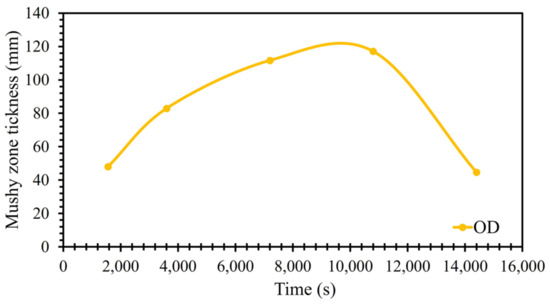
Figure 2.
The width of the mushy zone in the initial design during solidification.
To substantiate the accuracy of numerical computations, an assessment of the elemental concentration balance was conducted at various time steps following the solidification. The presentation of the mass balance during the simulation involved calculating the cumulative sum of both local and nominal concentrations for all elements at the total node after the simulation period. The outcomes, specifically those relating to the concentration balance for chromium (Cr), manganese (Mn), and molybdenum (Mo), are systematically provided in Table 3. Additionally, Figure 3 graphically depicts the temporal evolution of carbon (C) concentration during the solidification process at the location indicated by a red circle. As depicted in Figure 3, the hot liquid reaches the indicated location in the ingot at around 1000 s after pouring. Following this point, fluctuations in the concentration of carbon atoms are observed until approximately 14,000 s after pouring. At this juncture, the curve depicting the concentration of carbon stabilizes, which is indicative of the complete solidification of the liquid. The solid front reaches a specific point (as indicated in Figure 3) at 5800 s after pouring, coinciding with the local temperature reaching the local liquidus temperature. After this point, solidification initiates. The concentration of carbon at the indicated point (Figure 3) is influenced by the complex interplay between solidification kinetics, segregation phenomena, and fluid flow dynamics within the molten metal. Fluid flow within molten metal during solidification, such as natural convection or turbulent mixing, can influence the distribution of solute elements. Variations in fluid flow patterns can result in non-uniform mixing of carbon throughout the ingot, contributing to differences in carbon concentration at the indicated location. Additionally, in the mushy state, thickness increases as the cooling rate slows down. According to Figure 2, it then starts to decrease. In the mushy state, due to interdendritic liquid movement in the mushy zone, solute transfer, and the diffusion of solute elements in the solid state at each time step, there is a non-uniform distribution of carbon atoms between the solid and liquid phases, resulting in fluctuations in carbon concentration.
Table 3.
Cumulative sum of elemental concentrations in total nodes after solidification.
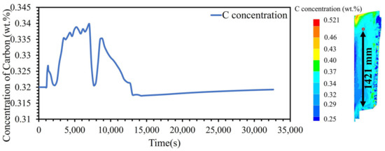
Figure 3.
Evolution of carbon concentration during solidification at the location indicated by a red circle.
Boundary Conditions and Input Parameters
In this study, a fourth of the geometry around the vertical axis was used for to perform simulations based on ingot symmetry. The material used in this study was AISI 4130 medium carbon steel of a low-alloy grade. The temperature-dependent thermo-physical properties such as density, specific heat, and solidus and liquidus temperatures were calculated using material analysis software JMatPro®, version 11.0 [32]. Heat transfer equations are solved for each subdomain with appropriate boundary conditions. The boundary conditions for ingot assembly include the following: (i) insulation at the free surface of the exothermic cap, (ii) insulation at the hot-top and riser, (iii) convection and radiation at the mold outer wall, (iv) initial convection and radiation after air-gap formation, followed by contact resistance between solid metal and the mold wall, and (v) contact resistance between mold components. The thermal boundary conditions are shown in Table 4.
Table 4.
Thermal boundary conditions [23].
4. Hot-Top Designs
Four different hot-top designs (Table 5), labeled ND1 to ND4, were investigated based on the variation in the thermal regime of the hot-top compared to the original design, designated OD. The original design is characterized by a partial sideboard (refractory) that covers the upper part of the hot-top with a thermal conductivity of 1.23 W/m/K (Figure 4a). The main characteristics of each of the new designs compared to the original one can be summarized as follows: in ND1, the hot-top is preheated to 200 °C (Figure 4b); in ND2, shown in Figure 4c, the type of refractory material is changed to reduce the thermal conductivity of the sideboard material to 0.45 W/m/K; and for ND3 and ND4 (Figure 4d and Figure 4e, respectively), an additional sideboard (extra refractory) with a height of 177 mm and a thermal conductivity of 1.23 W/m/K is added inside the hot-top. The new sideboard is placed below the previous sideboard. However, for ND4, the type of upper refractory is changed, and thermal conductivity is reduced to 0.45 W/m/K. Figure 4 illustrates the original version and the four newly proposed designs.
Table 5.
The hot-top specification in different designs.
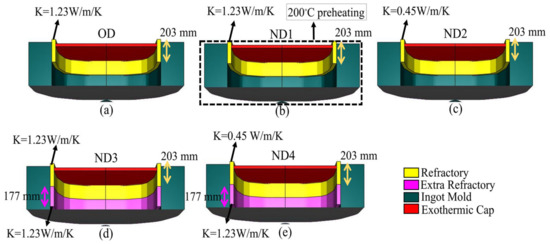
Figure 4.
(a) Original design: OD, (b) ND1, (c) ND2, (d) ND3, and (e) ND4.
5. Results and Discussions
In this section, we delve into the profound impact of changes in the hot-top thermal regime on crucial solidification parameters, covering solidification time (Section 5.1), temperature, and heat exchange (Section 5.2). The thermal field governs the solidification process [5,6,25], and the interplay of temperature gradients, fluid flow, and solute redistribution contributes to the formation of macrosegregated zones in castings or solidified metal structures [5,6,25]. Thus, a comprehensive understanding of the variations in solidification time, temperature gradient, and heat flux within the body of the ingot, occurring due to alterations in the hot-top thermal regime, is imperative. In conclusion, the ensuing section, Section 5.3, reports on the observed variations in terms of macrosegregation. Understanding and controlling these factors is crucial in the production of high-quality and homogeneous castings.
5.1. Solidification Time
If solidification time, which is a crucial parameter in ingot casting, is too short, there will be inadequate feeding to the central part of the ingot and increased porosity; conversely, a longer solidification time exacerbates segregation levels [15]. It is crucial to comprehend how solidification time varies with changes in hot-top design [15,19,33]. Figure 5 displays the total solidification time on the left side and the local solidification time on the right side, showing both the original design and the new designs of the hot-top. In this study, total solidification time refers to the local time required to reach the solidus temperature from the initial temperature at a specific location within the metal. On the other hand, the local solidification time represents the duration that passed between reaching the liquidus and solidus temperatures within the mushy zone [23]. Figure 5 reports the simulation results obtained at the end of solidification and reveals that the total solidification time is highly sensitive to variations in the thermal regime of the hot-top. Furthermore, Figure 5 illustrates that the quantity and progress of the local solidification time change notably, especially in the cases of ND3 and ND4. As indicated by the findings, a significant portion of the total solidification time is dedicated to the mushy state, and the local solidification time increases with the advancement of total solidification processes. The local solidification time correlates with the degree of microsegregation found within a growing crystal. When the local solidification time increases, this has a dual impact, inducing an increase in the diffusion time of solute elements in the solid state and an increase in the dendrite arm spacing value. Figure 6 shows the differences in total solidification time in terms of percentage for each of the designs in comparison with the original design. Merely preheating the hot-top up to 200 °C or using refractory material with lower thermal conductivity (0.45 W/m/K) results in a lower increase in the total solidification time than when the hot-top is completely covered with refractory material.
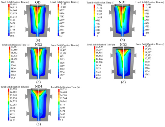
Figure 5.
The total solidification time on the left side and the local solidification time on the right side. (a) OD, (b) ND1, (c) ND2, (d) ND3, and (e) ND4.
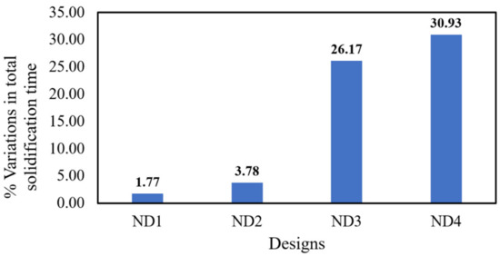
Figure 6.
Percentage differences in total solidification time for each design in comparison with the original design.
Figure 5d,e additionally demonstrate how the total solidification time profile changed in the hot-top and the core part of the ingot. It should be noted that the profile of the local solidification time significantly changed across nearly the entire ingot. The increase in the total solidification time of each new design compared to the OD in the center and the hot-top regions (red to the green contour) is shown in Figure 7. The largest increase in total solidification time was observed in the red, green, and yellow profiles, respectively, for both the hot-top and the centerline. Thus, the liquid metal that was placed in the hot-top region (especially in ND3 and ND4) remained in a liquid and mushy state for a longer time, leading to more liquid feeding from the hot-top towards the central parts of the ingot. The solidification profile was changed due to a lower solidification rate, especially in the centerline and hot-top. The results in Figure 7 show that variations in the thermal regime of the hot-top created a uniform trend of increasing the total solidification time compared with the OD. The variation in terms of heat exchange in the molten metal with the solid front was the source of changes in solidification time. Figure 8 shows the heat flux at the end of solidification in the radial direction from the center to the surface at height of 1679 mm and 820 mm from the bottom of the ingot (in the hot-top and middle of the ingot, respectively). As reported in Figure 8a, in general, ND3 and ND4 show less heat flux compared to OD. For example, at a distance of 140 mm from the center towards the wall in the radial direction (from r = 140 mm to r = 480 mm), this reduction was up to 11,319 W/m2 and 10,650 W/m2 for ND3 and ND4, respectively, compared to OD. In addition, an increase in heat flux to 3338 W/m2 and 3912 W/m2 for ND3 and ND4 was observed, respectively, compared to the OD in a radial direction up to 140 mm from the center (from r = 0 (center) to r = 140 mm). However, the direction of the heat flux vectors was toward the lower central part of the ingot. Therefore, the extension in the total solidification time in the hot-top area and the central part of the ingot occurred because of the lower heat transfer rate. The metal stayed in the liquid state or mushy state for a longer time, resulting in the continuous liquid feeding from the hot-top toward the center carrying on for a longer time due to an increase in the thermal regime (thermal capacity) of the hot-top. The reduction in positive segregation, observed in the hot-top region and the upper half of the ingot as presented in Section 5.3, coincided with variations in both total and local solidification times, particularly within the mentioned areas, as evidenced by the data shown in Figure 5. Furthermore, as illustrated in Figure 8a, there was a notable decrease in heat flux approximately 140 mm from the center towards the wall in the radial direction. This was particularly noticeable in the ND3 and ND4 configurations. This reduction in heat flux, which prolonged the local solidification time, appeared to be correlated with regions exhibiting reduced positive segregation. The declining trend in positive segregation could be attributed to the longer local solidification time, especially along the sidewall of the ingot. The extended residence time in the mushy state allowed for the increased diffusion of solute elements within the solid phase, resulting in decreased microsegregation between dendrite arm spacings. Additionally, in the later stages of solidification, when the centerline region of the hot-top was solidifying, an increase in local solidification time led to more segregation due to the increase in the dendrite arm spaces of equiaxed grains and the coarsening of equiaxed grains.
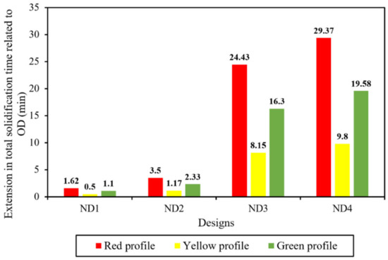
Figure 7.
The extension in total solidification time compared with OD in the center and hot-top areas (red, yellow, and green contours in Figure 5) for each of the designs.

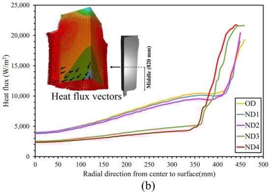
Figure 8.
The heat flux in the radial direction from the center to the surface (a) at the height of 1679 mm from the bottom of the ingot and (b) at the height of 820 mm from the bottom of the ingot.
5.2. Temperature
Understanding how the hot-top thermal regime affects temperature behavior across different parts of the ingot body is crucial, as the heat flux relies on the temperature gradient during solidification [34,35,36]. Hence, the local temperature of each node during solidification—from the filling step to the end of solidification—was calculated in the radial direction at various positions, including the bottom, middle, top, the interface of the hot-top/body, and the hot-top area. These calculations were performed for each design at specific heights, namely 253 mm, 790 mm, 1351 mm, 1612 mm, 1708 mm, and 1808 mm, respectively. The obtained values were compared to the ones in the OD to estimate the temperature difference between the OD and the new designs. The maximum temperature differences between the OD and ND1, ND2, ND3, and ND4 are reported in Figure 9. The results reveal a similar behavior in relation to the maximum value of temperature variation in the above-mentioned positions for each of the designs. An increasing trend was observed in the maximum value of temperature differences from the bottom toward the hot-top zone in each of the new designs when compared to the OD. The highest temperature difference values were observed at the hot-top, interface of the hot-top/body, and top of the ingot. In ND1, ND2, ND3, and ND4, the hot-top could maintain the molten metal liquid at higher temperatures of up to 37 °C (310.15 °K), 68 °C (341.15 °K), 264 °C (537.15 °K), and 306 °C (579.15 °K), respectively. It can be said that the changes in the heat extraction conditions produced by the new designs impacted the local temperature of the liquid. These observations are in agreement with those reported by other authors. Specifically, as Maduriya et al. [3] reported, temperature evolution indicates the effectiveness of heat transfer via the various interfaces of the ingot during solidification. Additionally, Patil et al. [37] reported that the temperature profile could be reliably used as a measure of heat transfer during solidification.
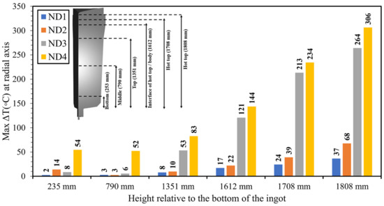
Figure 9.
The maximum value of the temperature difference in the radial direction for each of the designs in comparison with the OD at the bottom, middle, top, interface of the hot-top and body, and hot-top.
To analyze the impact of the hot-top thermal regime on the temperature profiles, the temperature distribution and heat flux were examined at the end of solidification. Figure 10 shows the temperature profile (right side) and heat flux pattern (left side) for each of the considered designs. When the thermal regime of the hot-top increases, there is an increase in the size of the contour domains of the temperature range from the bottom of the ingot body toward the hot-top area, with the temperature drop being lower in the wider contour. The results (Figure 10 and Figure 11) reveal that variation in hot-top heat capacity modifies the heat flux pattern over the entire ingot body and the hot-top. The distribution of the heat flux contours changes significantly when the thermal regime of the hot-top is changing, especially in ND3 and ND4 (ingot body center and top). The heat flux pattern changed in the zones near the hot-top wall and the center of the ingot body in ND1 and ND2 compared to the OD. The heat transfer magnitude changed greatly in the hot-top zone and ingot body when the hot-top was completely covered with refractory material. The maximum reduction in heat flux magnitude in the radial direction at a hot-top height of 1808 mm from the bottom of the ingot (Figure 11d) compared to the OD was estimated to be 20,185 W/m2 and 18,440 W/m2 in ND3 and ND4, respectively. These values were 8540 W/m2 and 6294 W/m2 in ND3 and ND4, respectively, at a height of 253 mm from the bottom of the ingot (Figure 11a). Thus, it is mostly the height of the sideboard and the thermal conductivity of the sideboard that significantly influence temperature evolution and heat transfer. Figure 11b–d depict the evolution of heat flux from the ingot wall up to a distance of approximately 200 mm from the ingot center in ND3 and ND4 configurations, with these arrangements showing lower values compared to other configurations. However, this trend is reversed in the vicinity of the center. According to the findings reported in Figure 9 and Figure 10, the temperature drop is less pronounced in the new configurations, particularly in ND3 and ND4, compared to the original design (OD). The variations in thermal conditions within the ingot, attributable to the hot-top thermal regime, have a significant impact on macrosegregation, as discussed in Section 5.3. The rate of heat removal governs the formation of solidification structures within the ingot. Typically, these structures consist of a chill zone, a columnar dendritic zone, and an equiaxed zone. The chill zone forms rapidly as the hot liquid steel comes into contact with the relatively cold mold wall, creating a high thermal gradient at the ingot surface. As solidification progresses, the structures transition to columnar dendritic structures due to the still-high thermal gradient, which acts as the driving force. However, as the thermal gradient decreases with further solidification, this driving force diminishes, and the structures become equiaxed toward the center of the ingot [36]. The reduced rate of heat extraction at the interface between the liquid metal and the hot-top components leads to the retention of molten metal at elevated local temperatures, particularly within the hot-top, the upper section of the ingot body, and at the interface of the hot-top/body. ND3 and ND4 configurations demonstrate a lower solidification rate, maintaining the required temperature gradient for columnar growth for a longer duration at the solidification front. Consequently, it can be inferred that there is a reduction in the area of the zone containing dendritic equiaxed grains in the centerline of the ingot. These alterations increase the negative segregation in the centerline while reducing the positive macorsegregation ratio, especially near the wall, in the radial direction. Due to the longer dwelling time when in the mushy state and the increased diffusion time of solute elements, there is a decrease in solute rejection toward the columnar tip. On the other hand, near the wall, the rejected solute elements are carried by fluid convection in the molten metal, resulting in a higher circulation and homogenization due to the expansion in the volume of the liquid pool at a higher temperature.
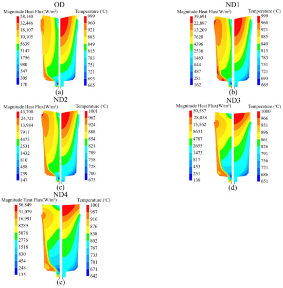
Figure 10.
Temperature profile at the right side and heat flux profile at the left side at the end of solidification (100% solidification), indicating the rate of heat transfer during solidification for (a) OD, (b) ND1, (c) ND2, (d) ND3, and (e) ND4.
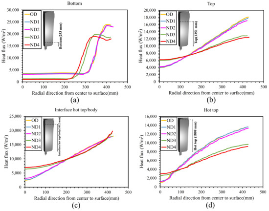
Figure 11.
Heat flux behavior in the radial direction from the center to surface (a) bottom of ingot, (b) top of ingot, (c) interface hot-top/body of ingot, and (d) hot-top.
5.3. Macrosegregation
The partitioning of solutes between the solid and liquid phases during alloy solidification results in micrometer-scale changes in composition. Density gradients induced by temperature-related and compositional changes in the liquid generate convective flows, where thermosolutal convection is the dominant mechanism for positive segregation and a contributor to the formation of negative segregation [38].
The buoyancy term of the momentum equation is shown in row 6 of Table 2. This value indicates the dependence of local density variation on thermal expansion, temperature gradients, solutal expansion, and concentration gradients in this model. Thus, the influence of the temperature gradient on the intensity of the macrosegregation ratio is computable in this model. Moreover, in the course of the solidification process, changes in density associated with phase transitions can result in the formation of density gradients within the material. These occurrences have the potential to cause specific components to migrate towards distinct regions, thereby contributing to macrosegregation. Furthermore, the density variations seen during phase transitions and solidification can induce convection and fluid flow within the material to compensate for shrinkage, thereby exacerbating the impacts of macrosegregation. The evolution of density is modeled as a function of the liquid and solid phases in the thermomechanical model employed in this study in order to account for thermosolutal transport, influenced by the combined effects of buoyancy- and shrinkage-induced flow [5,38,39].
As reported above, variation in the thermal regime of the hot-top caused a reduction in heat extraction (Figure 8 and Figure 11) between the liquid metal and hot-top components. This resulted in the molten metal remaining at a higher local temperature, especially in the hot-top, at interface of the hot-top/body, and in the top part of the ingot body, resulting in an increase in the total solidification time and the local solidification time. These changes also impacted the intensity of the macrosegregation ratio. The segregation ratio of carbon was calculated in the radial direction (from the center to 400 mm in the radial direction) of the hot-top, top, middle, and bottom of the ingot, and in the vertical direction (from the top to the bottom of the ingot) along the ingot centerline. The range of segregation, including maximum (Max) and minimum (Min) values, was determined at the above locations for each of the designs. Figure 12 shows the carbon segregation ratio in all the designs, which are arranged in terms of an increase in the total solidification time. According to the results, there is a decreasing trend in the maximum values of the carbon segregation ratio range in the bottom (Figure 12a), middle (Figure 12b), top (Figure 12c), hot-top (Figure 12d), and centerline (Figure 12e) of the ingot due to changes in the hot-top thermal regime. However, it is interesting to note that the evolution of the minimum segregation range does not follow a consistent trend for different designs. As discussed above, this could be due to an increase in local temperature, mostly in the hot-top and the upper region of the ingot body (Figure 9), leading to an increase in the total solidification time and local solidification time. In addition, as reported in Figure 7, the extension in total solidification times mostly occurs in the center and hot-top areas. Ghodrati et al. [3,4] reported that a 2.5% improvement in the solidification time resulted in a lower cooling rate in the mushy state, which led to more diffusion of solute elements in the solid state, and therefore a reduction in the solute rejection in the liquid. The reduction in the positive segregation ratio in the above-mentioned positions could be interpreted in terms of a longer diffusion time of solute elements into the solid state in the new designs compared to the OD.

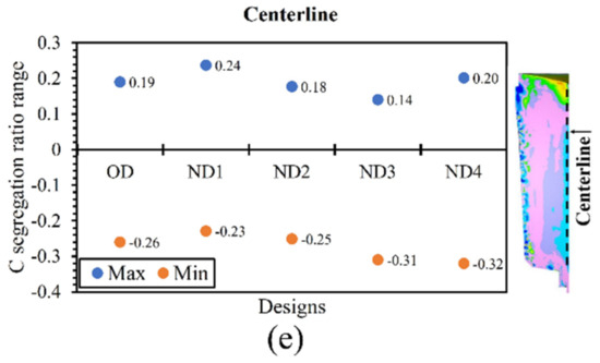
Figure 12.
Carbon macrosegregation ratio range including max and min in (a) radial direction in the bottom zone of ingot, (b) radial direction in the middle part of ingot, (c) radial direction in the top part of ingot, (d) radial direction in hot-top region, and (e) vertical direction in the center of the ingot.
Figure 13a shows the segregation ratio profile for carbon in the OD, ND1, ND2, ND3, and ND4 at the end of solidification. The negative segregation cone at the bottom and an accumulation of positive segregation at the hot-top region (which are typical forms of macrosegregation) were predicted well in each design. Negative segregation, or in other terms solute-poor regions, occurred along the side walls of the hot-top, as described rarely by some sources [20,24]. According to the simulation results reported in Figure 13b, the formation of negative segregation appears to have started at the very early stage of solidification during the filling process. Figure 13b shows the liquid fraction on the right side and the carbon segregation ratio on the left side at the end of the filling. In fact, a large drop in temperature is expected when the liquid metal comes into contact with the mold wall. This results in a significantly increase in the temperature gradient and hence a reduction in the size of the mushy zone. Pickering et al. [38] reported that, when the size of the mushy zone is reduced, solute-poor regions are produced upon solidification, thereby forming negative segregation bands. Figure 13c shows the experimentally measured carbon segregation map of the hot-top. The presence of negative segregation in the hot-top region was observed experimentally, which confirmed the simulation results. On the other hand, as indicated in Figure 13a, a notable reduction was observed in the volume of negative segregation (depicted by the dark blue area) that accumulated along the side wall of the hot-top when it was fully covered by the sideboard in ND3 and ND4 configurations. In these cases, the hot liquid came into direct contact with the sideboard wall instead of the mold wall, resulting in a lower temperature gradient at the interface between the sideboard wall and the liquid. We have ordered the segregation profiles for the four designs by the increasing trend in solidification time. The pink and purple patterns are related to 5% and 10% of segregation ratios, respectively. The area corresponding to the 5% segregation ratio (pink areas) extends into the hot-top zone in ND3 and ND4 designs. The results reveal also that the area with positive segregation (green and yellow zones) in the hot-top was reduced in size when the solidification time increased. Moreover, the position of positive segregation in the hot-top moved higher toward the metal surface. As reported in our previous studies [3,4], by delaying the process of solidification and slowing down the metal’s cooling rate, the height of the solidification shrinkage in the hot-top region can be reduced. Thus, the shrinkage cavity depth was decreased, and there was an upward movement in the accumulation of solute enrichment in the hot-top. The maximum displacement of the metal surface in the hot-top, due to contraction, was 158 mm, 156 mm, 140 mm, 101 mm, and 94 mm in OD, ND1, ND2, ND3, and ND4, respectively. Our effort to understand the material yield of the designs was conducted using top discard analysis to ensure there was not an intense segregation ratio. Bottom discards were not considered in this study. It is assumed that areas in the hot-top with carbon segregation greater than 10% must be removed to flatten the top surface of the ingot. The weight of discarded material in the hot-top part in relation to the total weight of the ingot material was calculated as a percentage of waste material. Then, the reduction in the percentage of waste material in the hot-top relative to the OD was calculated for each new configuration as a measure of material utilization efficiency. The waste material was 2188 kg, 1975 kg, 1542 kg, 1666 kg, and 1642 kg in OD, ND1, ND2, ND3, and ND4, respectively. As a result, with the new hot-top designs, material utilization efficiency rose to 9.7%, 29.5%, 23.9%, and 24.9% in ND1, ND2, ND3, and ND4, respectively.
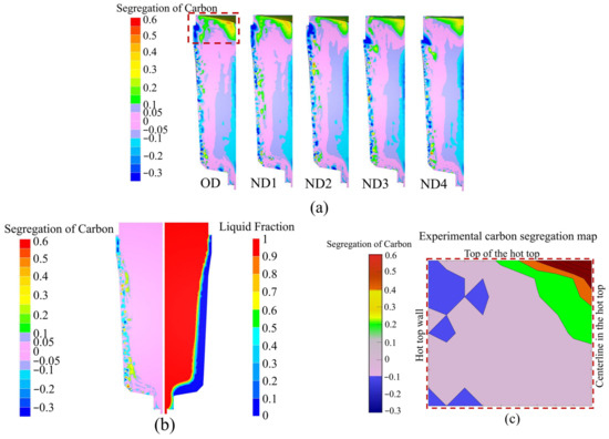
Figure 13.
(a) The carbon segregation ratio profiles of OD, ND1, ND2, ND3, and ND4 at the end of solidification; (b) carbon segregation ratio and liquid fraction profiles at the end of filling; (c) experimental carbon segregation ratio map in the hot-top, where the position of (c) is marked with the red box.
6. Conclusions
In this study, the influence of variation in the hot-top thermal regime on total solidification time, temperature, and heat flux, which impact the macrosegregation severity, was quantitatively investigated in a large-size cast ingot of 4130 medium-grade carbon steel. The results that could be drawn were as follows:
- Increments of approximately 2% to 31% were observed in the solidification time with changes made to the hot-top’s heat capacity.
- Inserting the additional sideboard in ND3 and ND4 configurations increased the total solidification time by approximately 30 min in the hot-top region and by up to about 20 min along the centerline axis of the ingot.
- When the hot-top was fully coated with refractory material, this resulted in decreased heat transfer in both the hot-top zone and ingot body, leading to reduced temperature drops, influencing solidification dynamics, and decreasing segregation patterns in the hot-top and upper half of the ingot.
- A descending trend in the carbon macrosegregation range, particularly with regard positive segregation, was observed in various regions of the ingot. This trend coincided with an increase in local solidification time, which facilitated greater diffusion of solute elements within the solid phase, consequently leading to decreased segregation.
- The new designs allowed us to increase the hot-top material yield by between 10 to 29%, depending on the changes made to the hot-top thermal regime. This finding has significant practical implications as it allows researchers to reduce hot-top material waste caused by severe macrosegregation.
Author Contributions
Conceptualization, N.G.; methodology, N.G.; software, N.G.; validation, N.G. and J.-B.M.; formal analysis, N.G.; investigation, N.G.; resources, M.J. and J.-B.M.; data curation, N.G.; writing—original draft preparation, N.G.; writing—review and editing, N.G. and M.J. and H.C.; visualization, N.G.; supervision, M.J.; project administration, M.J.; funding acquisition, M.J. All authors have read and agreed to the published version of the manuscript.
Funding
This work was supported by the Natural Sciences and Engineering Research Council of Canada (NSERC) in the framework of a Collaborative Research and Development project (CRD) [Grant number 536444-18]. Finkl Steel-Sorel Co. for providing the material is greatly appreciated.
Data Availability Statement
Data are contained within the article.
Conflicts of Interest
Author Jean-Benoit Morin was employed by the company Finkl Steel—Sorel. The remaining authors declare that the research was conducted in the absence of any commercial or financial relationships that could be construed as a potential conflict of interest.
Nomenclature
| Symbols | Parameters |
| Cp | Specific heat capacity (J/kg/°C) |
| Diffusion coefficient of solute i in the liquid (mm2/s) | |
| fl | Liquid fraction |
| fs | Solid fraction |
| g | Gravitational acceleration (m/s2) |
| H | Enthalpy (J) |
| h | Heat transfer coefficient (W/m/°C) |
| hcv | Convective heat transfer coefficient (W/m/°C) |
| Ks | Viscoplastic consistency in the solid |
| k | Partition coefficient |
| Permeability | |
| Lf | Latent heat of fusion (kJ/kg) |
| m | Strain-rate sensitivity coefficient |
| T | Temperature (°C) |
| Tf | melting temperature for pure iron (°K) |
| n | Strain hardening exponent |
| P | Pressure (MPa) |
| q | heat flux (W/m2) |
| Req | Heat transfer resistance (W/m2/°C)−1 |
| R0 | Nominal heat resistance (W/m2/°C)−1 |
| Rair | Air-gap heat resistance (W/m2/°C)−1 |
| Rrad | Heat transfer resistance (W/m2/°C)−1 |
| Tref | Reference temperature (liquidus) (°C) |
| Text | Exterior environmental temperature (°C) |
| Tmold | Initial temperature of molds, powders, and refractory (°C) |
| Tm | Melting temperature of pure iron (°C) |
| ωi | Local concentration of solute i (wt%) |
| Original composition (wt%) | |
| Nominal concentration of solute i (wt%) | |
| Concentration of solute i in the liquid (wt%) | |
| Liquidus slope | |
| N | Number of solute elements |
| Fourier number | |
| ρ0 | Reference density (kg/m3) |
| Thermal expansion coefficient (/K) | |
| Solutal expansion coefficient of solute i (×10−2/wt%) | |
| Average velocity | |
| Von Mises equivalent flow stress (MPa) | |
| ηl | Dynamic viscosity of the liquid |
| Equivalent plastic strain rate | |
| Equivalent plastic strain | |
| ρ | Density (kg/m3) |
| λ | Thermal conductivity (W/m/K) |
| Ɛr | Emissivity |
| σr | Stephan–Boltzmann constant (5.776 × 10⁻⁸ W/m2/K) |
| σs | Yield stress (MPa) |
Appendix A
As mentioned above, the macrosegregation map of all alloy elements was plotted using the experimental chemical analysis data. Table A1 shows the carbon segregation ratio range in the radial direction at the top, bottom, and centerline of the ingot (locations related to Table A1 are marked in Figure A1). Figure A2 shows the manganese segregation percentage map, both experimentally and numerically. Conic negative segregation and the positive segregation were observed at the bottom and top of the ingot (Figure A2). The range of Mn segregation percentage in the radial direction is shown in relation to the hot-top, top, and middle parts of the ingot in Figure A2 and Table A2. Generally, very good agreement was observed between the prediction and experimental results. It must be noted that, in the segregation model, the sedimentation of the equiaxed grains was not taken into consideration as it had little impact on carbon macrosegregation, and as doing so would induce a significant increase in computational time. Furthermore, difficulties were encountered in measuring the chemical composition of the edges of the sample in experimental measurements, and we lost the wall surface samples during the cutting process. The two abovementioned factors contribute to the differences observed for some conditions between the predicted and experimental results.
Table A1.
Carbon segregation ratio (experiment and simulation) at the end of solidification in the hot-top, bottom, and centerline of the ingot.
Table A1.
Carbon segregation ratio (experiment and simulation) at the end of solidification in the hot-top, bottom, and centerline of the ingot.
| Carbon Segregation Ratio | ||
|---|---|---|
| Locations | Experiment | Simulation |
| 1659 mm in height from the bottom (radial direction) | (−0.094, +0.5) | (−0.12, +0.41) |
| 90 mm in height from the bottom (radial direction) | (−0.12, +0.03) | (−0.12, +0.04) |
| 300 mm in height below the hot-top surface (vertical direction) | (+0.17, +0.57) | (+0.17, +0.56) |
| 600 mm in height above the bottom (vertical direction) | (−0.09, −0.04) | (−0.12, −0.03) |
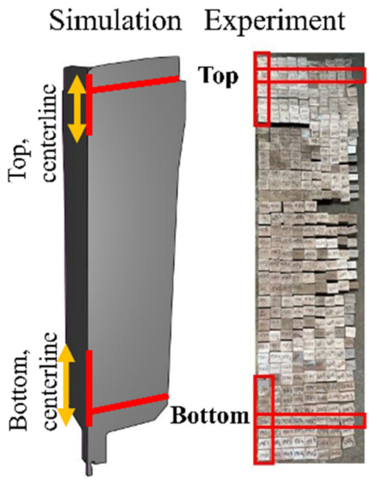
Figure A1.
The top, bottom, and centerline zones of the ingot (as indicated in the red lines and red boxes) were selected to analyze carbon segregation.
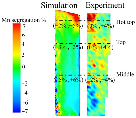
Figure A2.
Manganese segregation map (percentage): left side—simulation; right side—experiment.
Table A2.
Manganese segregation ratio (experiment and simulation) at the end of solidification in the hot-top, top, and middle of the ingot.
Table A2.
Manganese segregation ratio (experiment and simulation) at the end of solidification in the hot-top, top, and middle of the ingot.
| Manganese Segregation Ratio | ||
|---|---|---|
| Locations | Experiment | Simulation |
| Hot-top: 1708 mm in height from the bottom (radial direction from center to surface) | (0, +0.04) | (−0.02, +0.05) |
| Top: 1350 mm in height from the bottom (radial direction from center to surface) | (0, +0.04) | (−0.03, +0.03) |
| Middle: 790 mm in height from the bottom (radial direction from center to surface) | (−0.02, +0.04) | (+0.05, +0.06) |
References
- Pola, A.; Gelfi, M.; La Vecchia, G.M. Comprehensive Numerical Simulation of Filling and Solidification of Steel Ingots. Materials 2016, 9, 769. [Google Scholar] [CrossRef] [PubMed]
- Yu, S.; Zhu, L.Q.; Lai, J.H.; Pan, M.X.; Liu, Y.Y.; Xuan, W.D.; Wang, J.; Li, C.-J.; Ren, Z.-M. Application of heat absorption method to reduce macrosegregation during solidification of bearing steel ingot. J. Iron Steel Res. Int. 2022, 29, 1915–1926. [Google Scholar] [CrossRef]
- Maduriya, B.; Yadav, N. Prediction of solidification behaviour of alloy steel ingot casting. Mater. Today Proc. 2018, 5, 20380–20390. [Google Scholar] [CrossRef]
- Ghodrati, N.; Baiteche, M.; Loucif, A.; Gallego, P.I.; Jean-Benoit, M.; Jahazi, M. Influence of hot top height on macrosegregation and material yield in a large-size cast steel ingot using modeling and experimental validation. Metals 2022, 12, 1906. [Google Scholar] [CrossRef]
- Ludwig, A.; Wu, M.; Kharicha, A. On macrosegregation. Metall. Mater. Trans. A 2015, 46, 4854–4867. [Google Scholar] [CrossRef]
- Lesoult, G. Macrosegregation in steel strands and ingots: Characterisation, formation and consequences. Mater. Sci. Eng. A 2005, 413, 19–29. [Google Scholar] [CrossRef]
- Beckermann, C. Modelling of macrosegregation: Applications and future needs. Int. Mater. Rev. 2002, 47, 243–261. [Google Scholar] [CrossRef]
- Tveito, K.O.; Pakanati, A.; M’hamdi, M.; Combeau, H.; Založnik, M. A simplified three-phase model of equiaxed solidification for the prediction of microstructure and macrosegregation in castings. Metall. Mater. Trans. A 2018, 49, 2778–2794. [Google Scholar] [CrossRef]
- Li, J.; Xu, X.W.; Ren, N.; Xia, M.X.; Li, J.G. A review on prediction of casting defects in steel ingots: From macrosegregation to multi-defect model. J. Iron Steel Res. Int. 2022, 29, 1901–1914. [Google Scholar] [CrossRef]
- Isobe, K. Development Technology for Prevention of Macro-segregation in Casting of Steel Ingot by Insert Casting in Vacuum Atmosphere. ISIJ Int. 2021, 61, 1556–1566. [Google Scholar] [CrossRef]
- Hurtuk, D.J. Steel ingot casting. In Casting: ASM Handbook; ASM International Materials: Park, OH, USA, 2008; Volume 15, p. 911. [Google Scholar]
- Xu, Y.; Wang, Y.; Zhang, W.; Fei, T.; Zhang, Y.; Zhang, G. Simulation Analysis of Exothermic Powder in Riser Area on Inner Quality of Steel Ingot. IOP Conf. Ser. Mater. Sci. Eng. 2019, 631, 022070. [Google Scholar]
- Ghodrati, N.; Loucif, A.; Morin, J.B.; Jahazi, M. Modeling of the influence of hot top design on microporosity and shrinkage cavity in large-size cast steel ingots. In Proceedings of the 8th International Congress on the Science and Technology of Steelmaking, Montreal, QC, Canada, 2–4 August 2022; pp. 239–244. [Google Scholar] [CrossRef]
- Tashiro, K.; Watanabe, S.; Kitagawa, I.; Tamura, I. Influence of Mould Design on the Solidification and Soundness of Heavy Forging Ingots. Trans. Iron Steel Inst. Jpn. 1983, 23, 312–321. [Google Scholar] [CrossRef]
- Qian, S.; Hu, X.; Cao, Y.; Kang, X.; Li, D. Hot top design and its influence on feeder channel segregates in 100-ton steel ingots. Mater. Des. 2015, 87, 205–214. [Google Scholar] [CrossRef]
- Scepi, M.; Andreoli, B.; Basevi, S.; Giorgetti, A. Thermal and metallurgical control of the efficiency of ingot moulds for forging ingots. In Proceedings of the 9th International Schmiedetagung, Duesseldorf, Germany, 1 May 1981; pp. 77–82. [Google Scholar]
- Flemings, M. Principles of control of soundness and homogeneity of large ingots. Scand. J. Metall. 1976, 5, 1–15. [Google Scholar]
- Kumar, A.; Založnik, M.; Combeau, H.; Demurger, J.; Wendenbaum, J. Experimental and Numerical Studies on the Influence of Hot Top Conditions on Macrosegregation in an Industrial Steel Ingot. In Proceedings of the First International Conference on Ingot Casting, Rolling and Forging (IRCF), Aachen, Germany, 3–7 June 2012; pp. 3–7. [Google Scholar]
- Kermanpur, A.; Eskandari, M.; Purmohamad, H.; Soltani, M.A.; Shateri, R. Influence of mould design on the solidification of heavy forging ingots of low alloy steels by numerical simulation. Mater. Des. 2010, 31, 1096–1104. [Google Scholar] [CrossRef]
- Duan, Z.; Tu, W.; Shen, B.; Shen, H.; Liu, B. Experimental measurements for numerical simulation of macrosegregation in a 36-ton steel ingot. Metall. Mater. Trans. A 2016, 47, 3597–3606. [Google Scholar] [CrossRef]
- Zhang, C.; Loucif, A.; Jahazi, M.; Tremblay, R.; Lapierre, L.P. On the effect of filling rate on positive macrosegregation patterns in large size cast steel ingots. Appl. Sci. 2018, 8, 1878. [Google Scholar] [CrossRef]
- Matlab and Statistics Toolbox Release, The MathWorks, Inc.: Natick, MA, USA, 2012.
- Thercast® NxT 2.1 User Manual Ingot Casting.
- Wu, M.; Ludwig, A.; Kharicha, A. Volume-averaged modeling of multiphase flow phenomena during alloy solidification. Metals 2019, 9, 229. [Google Scholar] [CrossRef]
- Zhang, C. Influence of Casting Process Parameters on Macrosegregation in Large Size Steel Ingots Using Experimentation and Simulation. Doctoral Dissertation, École de Technologie Supérieure, University of Québec, Quebec City, QC, Canada, 2020. [Google Scholar]
- Gouttebroze, S.; Fachinotti, V.D.; Bellet, M.; Combeau, H. 3D-FEM modeling of macrosegregation in solidification of binary alloys. Int. J. Form. Process. 2005, 8, 203–217. [Google Scholar]
- Patil, P.; Puranik, A.; Balachandran, G.; Balasubramanian, V. FEM simulation of effect of mould wall thickness on low alloy steel ingot solidification. Ironmak. Steelmak. 2016, 43, 621–627. [Google Scholar] [CrossRef]
- Kim, N.Y.; Ko, D.C.; Kim, Y.; Han, S.W.; Oh, I.Y.; Moon, Y.H. Feasibility of Reduced Ingot Hot-Top Height for the Cost-Effective Forging of Heavy Steel Ingots. Materials 2020, 13, 2916. [Google Scholar] [CrossRef]
- Jaouen, O.; Costes, F.; Lasne, P. Finite element thermomechanical simulation of steel making from solidification to the first forming operations. In Proceeding of the 4th International Conference on Modelling and Simulation of Metallurgical Processes in Steelmaking, Columbus, OH, USA, 16–20 October 2011; pp. 10–20. [Google Scholar]
- Bellet, M.; Jaouen, O.; Poitrault, I. An ALE-FEM approach to the thermomechanics of solidification processes with application to the prediction of pipe shrinkage. Int. J. Numer. Methods Heat Fluid Flow 2005, 15, 120–142. [Google Scholar] [CrossRef]
- Zhao, X.; Zhang, J.; Lei, S.; Wang, Y. The Position Study of Heavy Reduction Process for Improving Centerline Segregation or Porosity With Extra-Thickness Slabs. Steel Res. Int. 2014, 85, 645–658. [Google Scholar] [CrossRef]
- JMatPro User’s Guide. 2005; Sente Software Ltd.
- Abootorabi, A.; Korojy, B.; Jabbareh, M.A. Effect of mould design on the Niyama criteria during solidification of CH3C 80t ingot. Ironmak. Steelmak. 2020, 47, 722–730. [Google Scholar] [CrossRef]
- Patil, P.; Puranik, A.; Balachandran, G.; Balasubramanian, V. Improvement in Quality and Yield of the Low Alloy Steel Ingot Casting Through Modified Mould Design. Trans. Indian Inst. Met. 2016, 70, 2001–2015. [Google Scholar] [CrossRef]
- Ge, H.; Ren, F.; Cai, D.; Hao, J.; Li, J.; Li, J. Gradual-cooling solidification approach to alleviate macrosegregation in large steel ingots. J. Mater. Process. Technol. 2018, 262, 232–238. [Google Scholar] [CrossRef]
- Malinowski, Z.; Telejko, M.; Hadała, B. Influence of heat transfer boundary conditions on the temperature field of the continuous casting ingot. Arch. Metall. Mater. 2012, 57, 325–331. [Google Scholar] [CrossRef]
- Patil, P.; Marje, V.; Balachandran, G.; Balasubramanian, V. Theoretical study on influence of steel composition on solidification behaviour in ingot casting of low alloy steels at similar casting conditions. Int. J. Cast Met. Res. 2015, 28, 117–128. [Google Scholar] [CrossRef]
- Pickering, E.J. Macrosegregation in steel ingots: The applicability of modelling and characterisation techniques. ISIJ Int. 2013, 53, 935–949. [Google Scholar] [CrossRef]
- Zhang, C.; Shahriari, D.; Loucif, A.; Melkonyan, H.; Jahazi, M. Influence of thermomechanical shrinkage on macrosegregation during solidification of a large-sized high-strength steel ingot. Int. J. Adv. Manuf. Technol. 2018, 99, 3035–3048. [Google Scholar] [CrossRef]
Disclaimer/Publisher’s Note: The statements, opinions and data contained in all publications are solely those of the individual author(s) and contributor(s) and not of MDPI and/or the editor(s). MDPI and/or the editor(s) disclaim responsibility for any injury to people or property resulting from any ideas, methods, instructions or products referred to in the content. |
© 2024 by the authors. Licensee MDPI, Basel, Switzerland. This article is an open access article distributed under the terms and conditions of the Creative Commons Attribution (CC BY) license (https://creativecommons.org/licenses/by/4.0/).