An Integrated Geometric and Hysteretic Error Model of a Three Axis Machine Tool and Its Identification With a 3D Telescoping Ball-Bar

Abstract

The ball-bar instrument is used to estimate a maximum number of hysteretic error sources. Machine error parameters include inter- and intra-axis errors as well as hysteresis effects. An error model containing cubic polynomial functions and modified qualitative variables, for hysteresis modeling, is proposed to identify such errors of the three nominally orthogonal linear axes machine. Such model has a total of 90 coefficients, not all of which being necessary. A numerical analysis is conducted to select a minimal but complete non-confounded set of error coefficients. Four different ball-bar test strategies to estimate the model coefficients are simulated and compared. The first one consists of circular trajectories on the primary planes XY, YZ, and XZ and the others use the XY plane, as an equator, and either four, five, or nine meridians. It is concluded that the five-meridian strategy can estimate the additional eight error coefficients: ECZ1, ECZ2, ECZ3, ECZb, EZY3, EZX3, ECX3, and ECXb. The Jacobian condition number is improved by increasing the number of meridians to 5. Further increasing the number of meridians from five to nine improves neither the number of estimable coefficients nor the conditioning, and so as it increases, the test time it was dismissed.

1. Introduction

The Cartesian volumetric error at the tool tip relative to the workpiece affects the quality of machined parts. Causes of such errors are inter- and intra-axis error parameters [1]. So, describing and identifying those errors play an important role in ensuring the machine tool performance through compensation or mechanical adjustments and repairs. For that purpose, several testing instruments were proposed such as the telescopic magnetic ball-bar [2,3,4,5], laser tracker interferometer [6], R-test [7], and touch trigger probe [8,9]. The telescopic magnetic ball-bar test is widely used to capture the linear axes errors by running a circular test on the plane of two axes [3] and to estimate machine error parameters [10]. It measures the deviations from a nominal circular trajectory as the volumetric error projected in the radial direction of the circular path [4]. Kunzmann et al. [11] proposed a ball-bar test to estimate positioning and squareness errors. Pahk et al. [12] used polynomials to model geometric errors. They used different terms of the polynomials to model positioning and straightness errors. Three circular tests, one for each pair of axes, yield 12 error coefficients plus three servo mismatch errors for the linear axes by their model. Mir et al. [5] proposed a theory and simulation to calibrate the five-axis machine tool link errors using ball-bar measurements. They constructed the sensitivity Jacobian matrix and applied the mathematical analysis, which yielded the reduced Jacobian. Jiang and Cripps [13] developed several ball-bar testing paths to identify the inter-axis errors of the rotary axes of a five-axis machine tool. They also used different ball-bar lengths to capture the orientation errors. Intra-axis errors of the rotary axes were estimated by running ball-bar tests on a five-axis machine tool with several circular patterns by Xiang and Yang [14]. They analyzed the effect of inter-axis and setup errors on measurement results. Slamani et. al. [15] modeled machine tool error parameters with degree optimized polynomials including motion hysteresis. They concluded that polynomials of degree three to four are appropriate for modeling the intra-axis errors.

Lee et al. [16] evaluated a machine tool accuracy by means of ball-bar measurements having various bar lengths and incorporating different machine tool feed rate. They ran the test for the base planes ZX, XY, and YZ and fitted a sphere to all data points using the least-square method. Then, they calculated the spherical deviations and the circular deviations to show that spherical analysis. It leads to a more reliable estimation and prediction than circular analysis since the former results in global optimization while the later results in local optimization. However, the spherical analysis is limited to using two axes at a time. Zhong et al. [17] proposed circular test paths considering different tool axis directions to evaluate the machine tool accuracy using spherical deviation modeling. They claimed that incorporating different tangential tool axis direction let the machine tool to reflect rotary axis errors in the measurements.

The main contribution of the work is to design different 2D and 3D telescoping ball-bar test strategies. The purpose is to identify a strategy by which a minimal but complete non-confounded set of error coefficients are provided using the numerical analysis. The proposed strategies involve the simultaneous motion of two or three linear axes thus resulting in volumetric errors that are the combination of many error sources. The novelty of the work is proposing a best ball-bar test strategy among several proposed models by which the number of the detectable machine error parameter modeled by cubic polynomials are improved from 29 to 37 in a single tool mode. The best strategy is experimentally tested on a machine tool. In Section 2, the forward kinematic model of the tested machine is described. Section 3 presents instructions to construct the Jacobian matrix considering the integrated error model. In Section 4, the mathematical analysis used to find the reduced Jacobian and set of non-confounded coefficients is discussed. In Section 5, different ball-bar test configurations are simulated and compared in terms of the Jacobian rank and condition number. In Section 6, the setup for the selected calibration strategy is explained and the results are presented and discussed. Finally, the conclusion follows in Section 7.

2. Forward Kinematic Modelling

A machine tool axes nominal motion, as well as geometric errors, are propagated through the kinematic chain. The relative inter-axis location errors, nominal axis motion, and intra-axis errors, representing the imperfection in the motion of an axis, are modeled by homogeneous transformation matrices (HTMs). Each machine axis is modeled by the consecutive multiplications of three HTMs describing the nominal link, between the preceding axis and the current one, the nominal axis motion and finally the intra-axis errors of the axis [18], e.g., Y, relative to its preceding neighbor, e.g., Z, as,

$${}^Z{T}_Y=T_{\mathrm{nominal}\mathrm{inter}-\mathrm{axis}\mathrm{location}}{T}_{\mathrm{nominal}\mathrm{motion}}{T}_{\mathrm{intra}-\mathrm{axis}\mathrm{error}}$$

(1)

Considering the target laboratory machine tool, it has a topology wCBXFZYSt where X, Y, and Z are the linear axes and B and C are the rotary axes. F is the machine tool frame located at the nominal intersection of B and C. w, S, and t are the workpiece, spindle, and the tool, respectively. T stands for the homogeneous transformation matrix (HTM). ${}^Z{T}_Y$ is the HTM of the Y-axis to the Z-axis. Considering that the rotary axes and the spindle are not used, the kinematic equation describing the location of the tool relative to the workpiece is,

$${}^w{T}_t={({}^F{T}_X{}^X{T}_w)}^{-1}({}^F{T}_Z{}^Z{T}_Y{}^Y{T}_t)$$

(2)

3. Integrated Error Model and Jacobian Matrix Generation

The three linear axes X, Y, and Z each contribute six intra-axis errors and together three out-of-squarenesses. Six setup errors including three translational errors for the ball-bar workpiece ball and three translational errors for the ball-bar tool ball are also added. The workpiece and tool orientations are not considered in this work. Each intra-axis error is modeled by cubic polynomials extended with a hysteresis term made of a real-valued error coefficient. It quantifies the hysteresis and a balanced ternary variable to apply it correctly depending on the known or unknown direction of motion to reach the current position [15]. So that,

$$E_{IH}=E_{IH0}+E_{IH1}h+E_{IH2}{h}^2+E_{IH3}{h}^3+{\dot{b}}_H{E}_{IH\mathrm{b}}$$

(3)

where E_IH is an intra-axis error, E_IH0, E_IH1, E_IH2, and E_IH3 are the coefficients of the polynomials. E_IHb is the hysteretic effect coefficient. The upper case I and H subscripts stand for the X-, Y- and Z-axis with different permutations. The lowercase variable h is a real number and stands for the H-axis position. Equation (3) is applied to all 18 intra-axis error parameters. The variable ${\dot{b}}_H$ is the sense of the motion defined as,

${\dot{b}}_H=+1$, for a forward movement in the X direction to reach the current position,

${\dot{b}}_H=-1$, for a backward movement in the X direction to reach the current position,

${\dot{b}}_H=0$, for an unknown sense of movement in the X direction to reach the current position.

The Jacobian matrix is generated using the HTMs of Equation (1), Equation (2), and small angular error approximations. It forms a linear system describing the sensitivity of the tool tip Cartesian volumetric error components to the machine intra-axis errors and the setup errors,

$$E_v=J\times E_p$$

(4)

where J is the Jacobian (3m × n) with m as the number of measured positions and n as the number of machine error parameters. E_v is the volumetric Cartesian error vector components column matrix and E_p is the machine error parameters and setup errors column matrix. Having modeled the intra-axis errors with polynomials and hysteretic terms, the Jacobian is further expanded to represent the sensitivity of the Cartesian volumetric error components to the intra-axis error coefficients and setup errors.

Table 1. All potential machine error coefficients for the three linear axes and the setup errors: With and without asterisks (*). The sufficient non-confounded error coefficients: with asterisks (*).

Error Parameters		Polynomial Coefficients (Polynomial Degree 3)				Hysteretic Errors
		E0	E1	E2	E3
X-axis errors	EXX	EXX0	EXX1 *	EXX2 *	EXX3 *	EXXb *
	EYX	EYX0	EYX1 *	EYX2 *	EYX3 *	EYXb *
	EZX	EZX0	EZX1 *	EZX2 *	EZX3 *	EZXb *
	EAX	EAX0	EAX1 *	EAX2 *	EAX3 *	EAXb *
	EBX	EBX0	EBX1 *	EBX2 *	EBX3 *	EBXb *
	ECX	ECX0	ECX1 *	ECX2 *	ECX3 *	ECXb *
Y-axis errors	EXY	EXY0	EXY1	EXY2 *	EXY3 *	EXYb *
	EYY	EYY0	EYY1 *	EYY2 *	EYY3 *	EYYb *
	EZY	EZY0	EZY1	EZY2 *	EZY3 *	EZYb *
	EAY	EAY0	EAY1	EAY2	EAY3	EAYb
	EBY	EBY0	EBY1	EBY2	EBY3	EBYb
	ECY	ECY0	ECY1	ECY2	ECY3	ECYb
Z-axis errors	EXZ	EXZ0	EXZ1 *	EXZ2 *	EXZ3 *	EXZb *
	EYZ	EYZ0	EYZ1 *	EYZ2 *	EYZ3 *	EYZb *
	EZZ	EZZ0	EZZ1 *	EZZ2 *	EZZ3 *	EZZb *
	EAZ	EAZ0 *	EAZ1 *	EAZ2 *	EAZ3 *	EAZb *
	EBZ	EBZ0	EBZ1	EBZ2	EBZ3	EBZb
	ECZ	ECZ0 *	ECZ1 *	ECZ2 *	ECZ3 *	ECZb *
Setup errors	EXw, EYw, EZw, EXt *, EYt *, EZt *

lists the initial 90 machine error coefficients and six setup errors.

4. Sufficient Set of Non-Confounded Error Coefficients

The 90-variable model and 6 setup errors are now analyzed for minimality and completeness. Minimality means that a minimum number of variables are used, which can completely represent the behavior of the system considering the relevant volumetric quantities, the tool geometry, and the machine poses. Here, a pose is a set of X-, Y-, and Z-axis coordinates and the volumetric quantities are only the Cartesian coordinates, not the orientation, of the tool relative to the workpiece. The Jacobian is generated for a random set of 8000 poses located on the X, Y, and Z working volume. The Jacobian has 96 columns, one per unknown coefficient, its rank is 59, and its condition number is 3.8 × 10³⁵. Therefore, a minimal model should have 59 independent variables (or columns). A set of variables is selected to provide the lowest possible condition number but favoring a set that makes geometric sense. So, both numerical quantities and geometric reasoning are used to prune variables off the initial Jacobian. The pruning proceeds as follows,

The workpiece ball setup errors, i.e., EXw, EYw, and EZw, are removed as they are confounded with the tool ball setup errors, i.e., EXt, EYt, and EZt, and the new Jacobian has 93 columns, a rank of 59, and a condition number of 3.8 × 10³⁴.

The first (zero-degree) terms of the polynomials for all the errors except EAZ0 and ECZ0, which model the out-of-squareness errors of the Y-axis, are confounded. The squareness error EA(0Z)Y of the Y-axis relative to the Z-axis around an axis parallel to the X-axis is modeled using intra-axis error coefficients EAZ0. 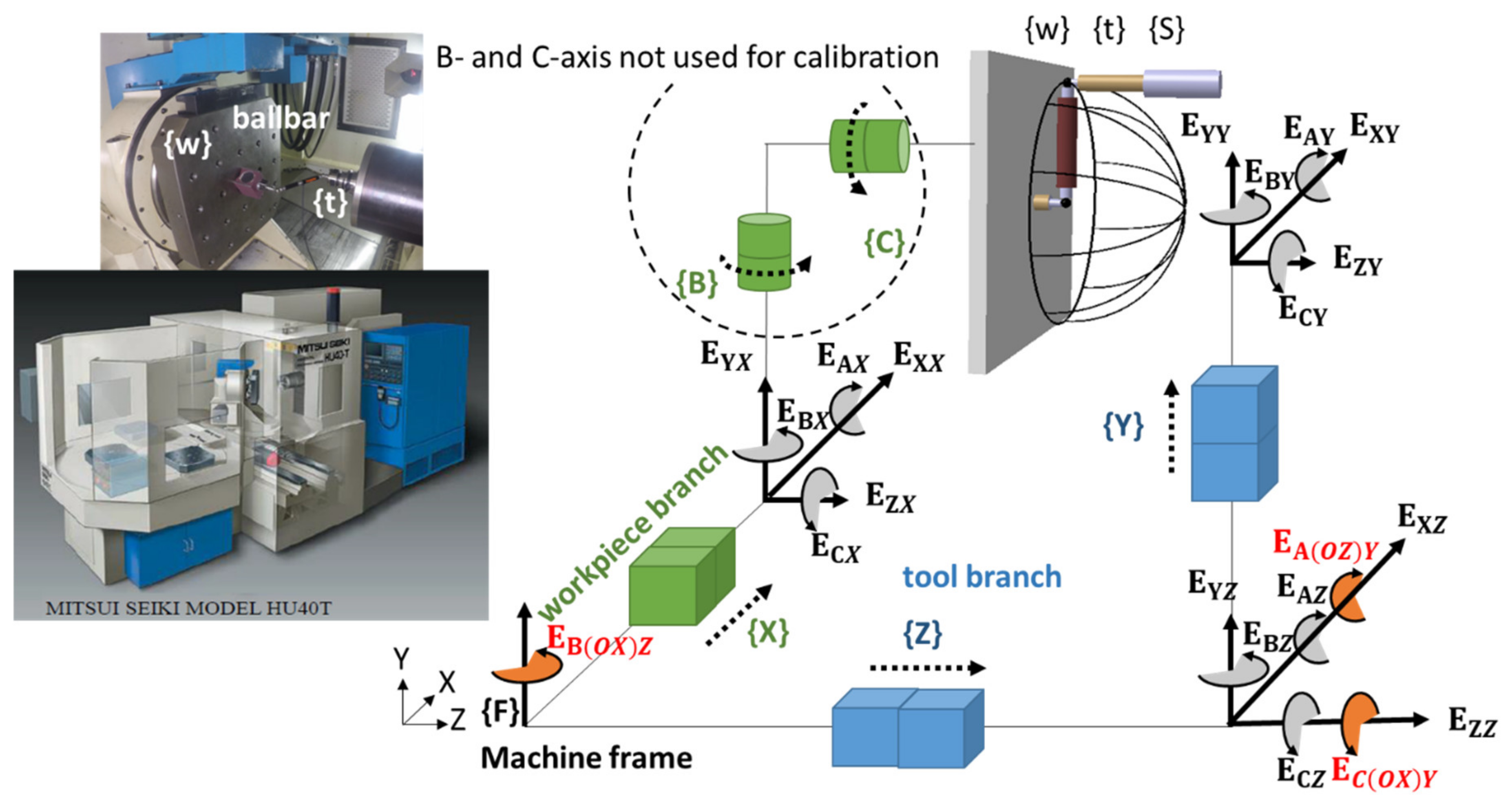The squareness errors EC(0X)Y of the Y-axis relative to the X-axis around an axis parallel to the Z-axis is modeled using intra-axis error coefficients ECZ0. So, a total of 16 error coefficients (EXX0, EYX0, EZX0, EAX0, EBX0, ECX0, EXY0, EYY0, EZY0, EAY0, EBY0, ECY0, EXZ0, EYZ0, EZZ0, EBZ0) are removed from the model because they have the same effect as the setup errors. The Jacobian rank is still 59 while now having 77 columns or variables. The machine tool schematic and the intra- and inter-axis errors are illustrated in Figure 1.

The angular error coefficients of the Y-axis cannot be estimated because a single tool geometry is used, which does not allow the linear system to distinguish between its linear and angular intra-axis errors. So, 12 error coefficients (EAY1, EAY2, EAY3, EAYb, EBY1, EBY2, EBY3, EBYb, ECY1, ECY2, ECY3, ECYb) are removed from the Jacobian. The Jacobian size, rank, and condition number become 65, 59, and 2.9 × 10²⁶, respectively.

Using only one tool length for the analysis causes the angular error of EBZ not to be distinguishable from the linear errors. So, by removing (EBZ1, EBZ2, EBZ3, EBZb) from the model the size, rank, and condition number become 61, 59, and 2.4 × 10²⁴, respectively.

The first-degree coefficients of the polynomials for the straightness errors are redundant because out-of-straightness is the departure from straightness and this first-degree term does not cause a departure from straightness. However, EXZ1 is intentionally kept because it can model the squareness error EB(0X)Z of the Z-axis relative to the X-axis around an axis parallel to the Y-axis. Since eliminating EXY1 from the model does not change the rank, it is removed from the model. The Jacobian size, rank, and condition number are 60, 59, and 2.5 × 10²⁴, respectively. The last confounded coefficient is EZY1, which is deleted from the model. The Jacobian becomes full rank, with a size of 59 and rank of 59. The non-normalized and normalized Jacobian condition numbers are 2.3 × 10¹¹ and 387, respectively. By deleting EYX1, EZX1, and EYZ1 one by one from the model, the Jacobian rank decreases to 56 while the normalized Jacobian condition number becomes 108.41.

Hence, to predict the volumetric error, 53 error coefficients plus 3 setup errors are required to be estimated (96 minus 40 redundancies), which represents the minimal and complete model shown by red color in Table 1. However, because the ball-bar test provides only the distances between the two balls, which is equivalent to projecting the Cartesian volumetric errors along the ball-bar axis, additional coefficients, which will be shown in the next section, will not be independently observable.

5. Ball-Bar Test Modelling (Simulation)

A typical ball-bar test is designed to measure the distances between two balls, the tool ball at the tool holder, and the workpiece ball on the machine pallet or table while the axes travel a nominally circular path. The circular paths can pass through the XY, YZ, and XZ planes, which only requires a circular interpolation. They involve the motion of two axes (2D ball-bar) or a combination of the three linear axes (3D ball-bar) for linear axes evaluation. The test strategy should estimate all machine error coefficients of the minimal and complete model in a minimum test time.

Table 2. Different configurations for the ball-bar test, Jacobian rank (J. rank) and Jacobian condition number (J. C. N.). Strategy 3D3: XY, XZ, and YZ plane, Strategy 3D5: XY, XZ, YZ plane, and two 45° meridians, Strategy 3D6: XY, XZ plane, and four 36° meridians, Strategy 3D10: XY, XZ plane, and eight 20° meridians.

	Strategy 1, 2D	Strategy 2, 3D5	Strategy 3, 3D6	Strategy 4, 3D10
Top view 3D view
J. rank	32	40	40	40
Jacobian not normalized condition number before pruning (J.C.N.)
	5.04 × 1028	3.7 × 1026	2.3 × 1026	3.4 × 1026
Jacobian normalized condition number after Pruning (J.C.N.)
	2801	1950	1948	1948

shows different test strategies as 2D ball-bar (XY, XZ and YZ plane), 3D5 ball-bar (XY, XZ, YZ plane, and two 45° meridians), 3D6 ball-bar (XY, XZ plane, and four 36° meridians), and 3D10 ball-bar (XY, XZ plane, and eight 20° meridians). The travels are bidirectional (back and forth) to capture hysteretic effects. To model the ball-bar test, all relative positions of the tool to the workpiece obtained by Equation (2) are projected along the sensitive direction of the ball-bar. A workpiece spherical coordinate system is defined located at the workpiece ball center attached to the table. Also, the Jacobian is projected along the sensitive direction of the ball-bar. For position i, J_i,projected is obtained by,

$$J_{i,projected}=\begin{array}{cc}[\sin {\theta }_i\cos {\varphi }_i& \begin{array}{cc}\sin {\theta }_i\sin {\varphi }_i& \cos {\theta }_i]J_i\end{array}\end{array}$$

(5)

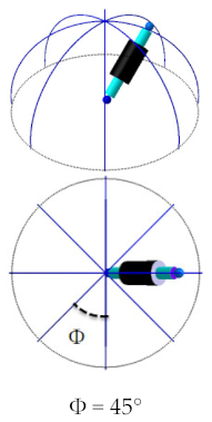
which presents the first partial derivatives of the ball-bar length variations to the machine error coefficients and the setup errors. J_i is the Jacobian for each position (3 × 1). The θ and ϕ are the polar and the azimuthal angle, respectively, illustrated in Figure 2. So, the error of the tool tip projected in the ball-bar direction, ρ, is related to the error coefficients as,

$$\rho =J_{projected}{E}_p$$

(6)

where $J_{projected}$ is the accumulated projected Jacobian for all the positions. To estimate machine error coefficients, an iterative Gauss–Newton method is applied on,

$$E_p=J_{projected}{}^{†}\rho$$

(7)

where $J_{projected}{}^{†}$ is the pseudo-inverse of the projected Jacobian matrix. The calculated error coefficients, after the first iteration, are used to predict the projected error using Equation (6). The iteration is continued until convergence to a negligible error coefficients change threshold in the iterative loop.

The first strategy, 2D ball-bar, gives a Jacobian with a rank of 32 (29 error coefficients plus 3 setup errors). However, the second, third, and fourth strategies, i.e., 3D5, 3D6, and 3D10, provide Jacobians with ranks of 40. The Jacobians condition numbers are 5.04 × 10²⁸, 3.7 × 10²⁶, 2.3 × 10²⁶, and 3.4 × 10²⁶ for the first, second, third, and fourth strategies, respectively. By comparing the ranks of the Jacobians, it is observed that by adding two 45° meridians to the first strategy (2D) to obtain the 3D5 strategy, the rank is improved to 40 (37 error coefficients plus 3 setup errors). However, adding more meridians to the third strategy does not improve the estimates, rank, and condition number for the fourth strategy. The second, third, and fourth strategies provide equal projected error information in the 3D volume, which is higher than the first strategy. The condition number and the rank of the Jacobians show that further error coefficient pruning is needed to eliminate the weakly contributing coefficients and obtain more reliable estimates of the error coefficients than when the Jacobian column size is 56. Pruning can be guided by a mathematical analysis including singular value analysis, condition number, and rank of the Jacobian. The procedure of eliminating the confounded coefficients for strategy 3D5, 3D6, and 3D10 are listed in

Table 3. The procedure to obtain the reduced Jacobians for the strategies, 3D5, 3D6, and 3D10.

Error Coefficients Removed	Number of Redudancies	Notes	J. Size	J. Rank	J. Condition Number
-	-	The results are for the minimal complete set of coefficients obtained for the machine model for a single tool in 3D Cartesian position mode. This set of coefficients is the starting point for the analysis of these ball-bar strategies. The size exceeds the rank by 16 coefficients.	56	40	Not-normalized Cond. 3D6: 3.3 × 1026
EAX1 EAX2 EAX3 EAXb EBX1,EBX2 ECX1,ECX2	8	For the ball-bar test, the angular errors of the X-axis cannot be separated from the linear errors. However, it is not preferable to remove the fourth (third-degree) terms and the backlashes of the EBX and ECX since those eliminations would decrease the rank.	48	40	Not-normalized Cond. 3D6: 3.3 × 1025
EAZ1 EAZ2 EAZ3 EAZb	4	Since the errors are projected in the sensitivity direction of ball-bar and the tool is in the Z direction, the angular error of the Z-axis around A cannot be distinguished from the linear errors in Y direction.	44	40	Not-normalized Cond. 3D6: 5.4 × 1023
EXX2	1	EXX2 is in part confounded with EXt.	43	40	Not-normalized Cond. 3D6: 1.2 × 1021
EYX3	1	EYX3 is in part confounded with EXY3.	42	40	Not-normalized Cond. 3D6: 1.9 × 1015
EYY2	1	EYY2 is in part confounded with EYt.	41	40	Not-normalized Cond. 3D6: 9.7 × 1014
EZZ2	1	EZZ2 is in part confounded with EZt.	40	40	Not-normalized Cond. 3D6: 1.3 × 1011 Normalized Cond. 3D6: 1948

. The Jacobians of the second and fourth strategies are reduced as for the third one. The normalized Jacobians condition numbers are 1950, 1948, and 1948 for the second, third, and fourth strategies, respectively.

The first strategy (2D) has the Jacobian rank and size of 33 and 40, respectively. Having exploited the reduced Jacobian in the second, third, and fourth strategies explained in Table 3, the procedure to achieve a full rank Jacobian for strategy 3D3 is as follows,

While less information is provided by a 2D ball-bar test strategy, the error coefficients ECZ1, ECZ2, ECZ3, and ECZb for the angular error parameter ECZ are deleted from the model. Therefore, rank, size, and condition number are 33, 36, and 3.2 × 10²⁶.

EZY3 is in part confounded with EYZ3. Therefore, removing EZY3 from the model results in a Jacobian with a rank, size, and condition number 33, 35, and 2.1 × 10²⁶.

By deleting EZX3, which is in part confounded with EXZ3 from the Jacobian, its rank, size, and condition number become 33, 34, and 2.8 × 10²⁵.

One more coefficient should be removed. Although removing ECZ0 from the model results in the Jacobian being full rank (rank of 33) with the normalized Jacobian condition number of 3118, it is preferable to keep this coefficient in the model because it models the out-of-squareness of EC(0X)Y. By analyzing the Jacobian, it is observed that by removing the error coefficients of ECX3 and ECXb for the angular error parameter ECX, the Jacobian becomes full rank (rank of 32) while having 32 columns. The non-normalized and normalized Jacobian condition numbers become 1.49 × 10¹¹ and 2801, respectively. Therefore, 29 error coefficients plus 3 setup errors are the output of this strategy. The non-confounded error coefficients in 3D ball-bar test while having one tool length and one ball-bar length for all four strategies are shown in

Table 4. Non-confounded error coefficients in 3D ball-bar test using strategies 3D5, 3D6, and 3D10: With and without asterisks (^*). Non-confounded error coefficients in strategy 2D: with asterisks (^*).

Error Parameters		Retained Polynomial Coefficients for Degrees 0 to 3				Hysteretic Error Coefficients
		0	1	2	3
X-axis errors	EXX		EXX1 *		EXX3 *	EXXb *
	EYX			EYX2 *		EYXb *
	EZX			EZX2 *	EZX3	EZXb *
	EAX
	EBX				EBX3 *	EBXb *
	ECX				ECX3	ECXb
Y-axis errors	EXY			EXY2 *	EXY3 *	EXYb *
	EYY		EYY1 *		EYY3 *	EYYb *
	EZY			EZY2 *	EZY3	EZYb *
	EAY
	EBY
	ECY
Z-axis errors	EXZ		EXZ1 *	EXZ2 *	EXZ3 *	EXZb *
	EYZ			EYZ2 *	EYZ3 *	EYZb *
	EZZ		EZZ1 *		EZZ3	EZZb *
	EAZ	EAZ0 *
	EBZ
	ECZ	ECZ0 *	ECZ1	ECZ2	ECZ3	ECZb
Setup errors	EXt *, EYt *, EZt *

.

Among different ball-bar test strategies simulated, the third strategy is selected as the best strategy because it has a Jacobian with a higher rank than the first one. On the other hand, in terms of considering the minimum test time, it is preferred over the 3D10 strategy. The preference of strategy 3D6 over 3D5 is because the third strategy generates a Jacobian with a lower condition number than the second strategy. However, 3D5 and 3D10 strategies could be also useful since the rank of generated Jacobian are as the same as strategy 3D6.

6. Experimental Test and Discussions

The third strategy is selected for experimental trials for validation. The ball-bar has a measuring range of around 1 mm. So, the test path aims to keep the ball to ball distances nominally constant. A circular path is usually programmed. Therefore, by running the test, the ball attached to the tool travels on an arc in a space centered on the workpiece ball. The tested machine is a five-axis horizontal machining center produced by Mitsui Seiki model HU40-T, with ball screw feed-drive systems, and a 150i-M Fanuc controller. The nominal ball-bar length is 150 mm. Figure 3 shows the test setup. Writing the G-code for the test requires calculating the joint positions for points on the meridians and equator using Cartesian coordinate retrieved from the spherical coordinates incorporating the machine tool kinematic model. The number of measurements depends on the sampling rate of the ball-bar software, which depends on the declared feed rate. G-code command G01 is used. The number and positions of ball-bar length readings may not match the positions programmed in the G-code because there is no synchronization between the machine motion and the ball bar readings, except that the start of the G-code program is detected via the initial radial engagement of the ball-bar as for a classic ball-bar test. Hence, the positions locations, whose errors are captured by the test, are estimated, not measured. The feed rate is set to 500 mm/min and is kept constant. A total of 5990 distance readings are acquired by the ball-bar test. The hysteretic error compensation was deactivated in the machine tool controller. The room temperature was 21 °C during the test. The test was repeated five times over five consecutive days while the machine was in similar environmental conditions. Each test lasted 37 min without considering setup time, which was around 20 min.

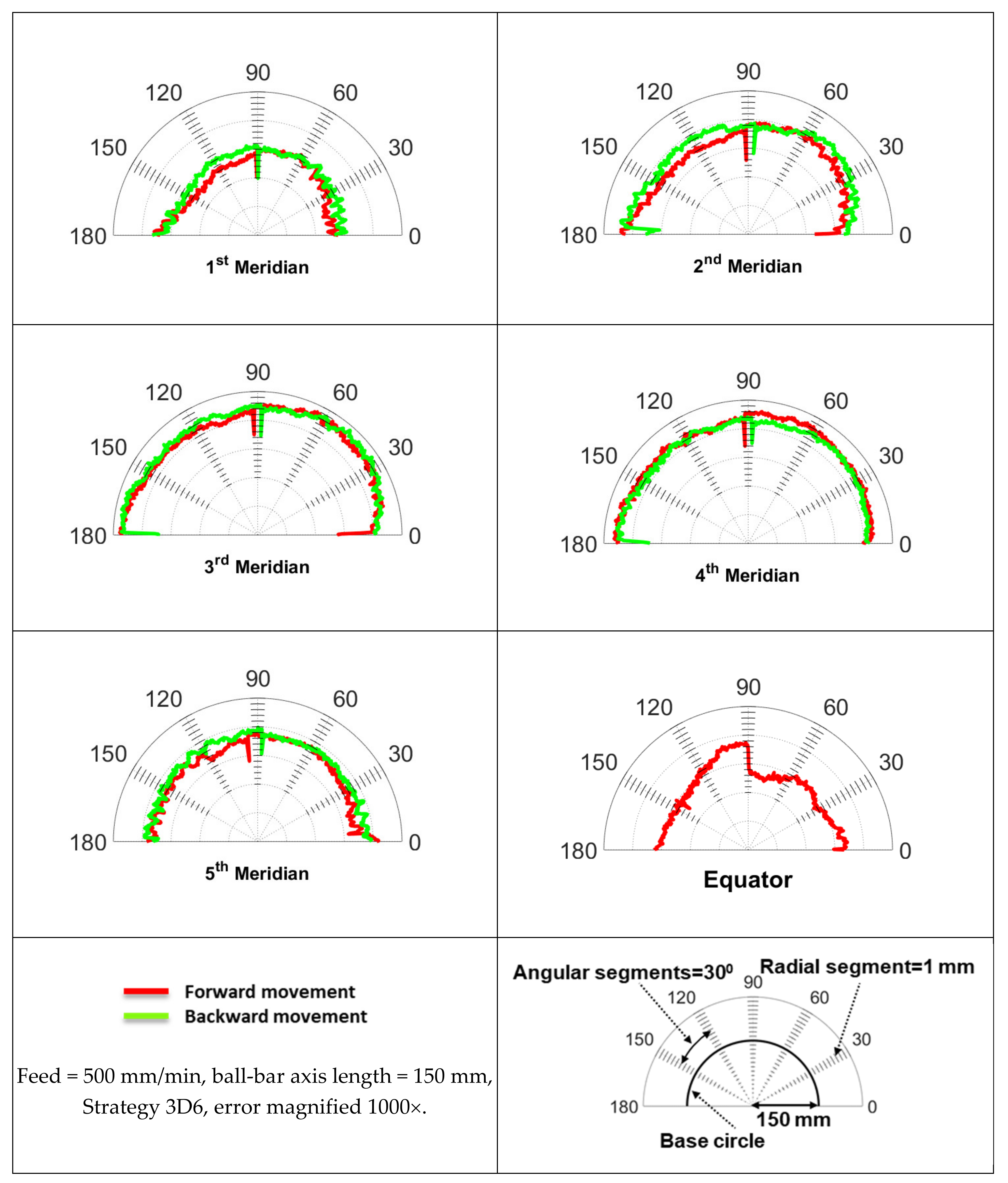
The experimental ball-bar measurements for the strategy 3D6 are shown in Figure 4 for the movements along the meridians. Each polar plot contains the measurement data of the forward and the backward movements. The errors are magnified 1000 times. Each segment is equal to 1 µm.

Once the 3D ball-bar tests information is gathered, they are injected into the model (Equation (6)) to estimate the machine error coefficients. The test was repeated five times with each data set processed separately, thus providing mean and standard deviations of the estimated model coefficients given by,

$$s_i(E_p{}_i)=\sqrt{\frac{1}{n-1}{\displaystyle \sum _{j=1}^n{(E_{pij}-{\overline{E}}_p{}_i)}^2}}$$

(8)

where $E_{pij}$ is ith error parameter for the jth run. j = 1 to 5 and i = 1 to 37.

Table 5. Estimation results for the error coefficients values and their standard deviation.

Coefficient	Estimated Results	Standard Deviation	Coefficient	Estimated Results	Standard Deviation
EXX1 (mm/mm)	−6.96 × 10−6	2.5 × 10−6	EZY3 (mm/mm3)	2.34 × 10−9	3.7 × 10−10
EXX3 (mm/mm3)	3.64 × 10−10	1.7 × 10−10	EZYb (mm)	−5.24 × 10−4	4.7 × 10−4
EXXb (mm)	4.81 × 10−4	1.6 × 10−4	EXZ1 (mm/mm)	3.94 × 10−5	3.5 × 10−6
EYX2 (mm/mm2)	−8.25 × 10−8	2.4 × 10−8	EXZ2 (mm/mm2)	−3.74 × 10−7	3.5 × 10−8
EYXb (mm)	−4.54×10−4	1.0 × 10−5	EXZ3 (mm/mm3)	1.16 × 10−9	4.7 × 10−10
EZX2 (mm/mm2)	5.99 × 10−7	3.9 × 10−8	EXZb (mm)	−1.37 × 10−4	3.9 × 10−6
EZX3 (mm/mm3)	2.05×10−9	3.9 × 10−10	EYZ2 (mm/mm2)	−6.59 × 10−8	1.4 × 10−8
EZXb (mm)	3.91 × 10−5	1.08 × 10−5	EYZ3 (mm/mm3)	9.88 × 10−10	8.8 × 10−11
EBX3 (rad/mm3)	5.71 × 10−11	1.7 × 10−11	EYZb (mm)	6.07 × 10−5	8.1 × 10−6
EBXb (rad)	−0.0023	3.3 × 10−5	EZZ1 (mm/mm)	3.79 × 10−5	5.9 × 10−7
ECX3 (rad/mm3)	8.1 × 10−10	1.4 × 10−10	EZZ3 (mm/mm3)	−9.68 × 10−10	2.4 × 10−11
ECXb (rad)	0.0018	6.6 × 10−5	EZZb (mm)	5.01 × 10−4	3.3 × 10−5
EXY2 (mm/mm2)	2.74 × 10−8	3.4 × 10−9	EAZ0 (rad)	−9.44 × 10−5	1.0 × 10−5
EXY3 (mm/mm3)	−4.01×10−10	1.66×10−10	ECZ0 (rad)	2.48×10−4	3.2×10−6
EXYb (mm)	2.24 × 10−5	6.88 × 10−6	ECZ1 (rad/mm)	−5.21 × 10−6	2.2 × 10−7
EYY1 (mm/mm)	1.06 × 10−4	1.85 × 10−5	ECZ2 (rad/mm2)	3.56 × 10−8	3.8 × 10−9
EYY3 (mm/mm3)	−2.78 × 10−9	3.58 × 10−10	ECZ3 (rad/mm3)	−8.01 × 10−11	2.5 × 10−11
EYYb (mm)	−0.0031	1.49 × 10−4	ECZb (rad)	1.83 × 10−5	8.1 × 10−6
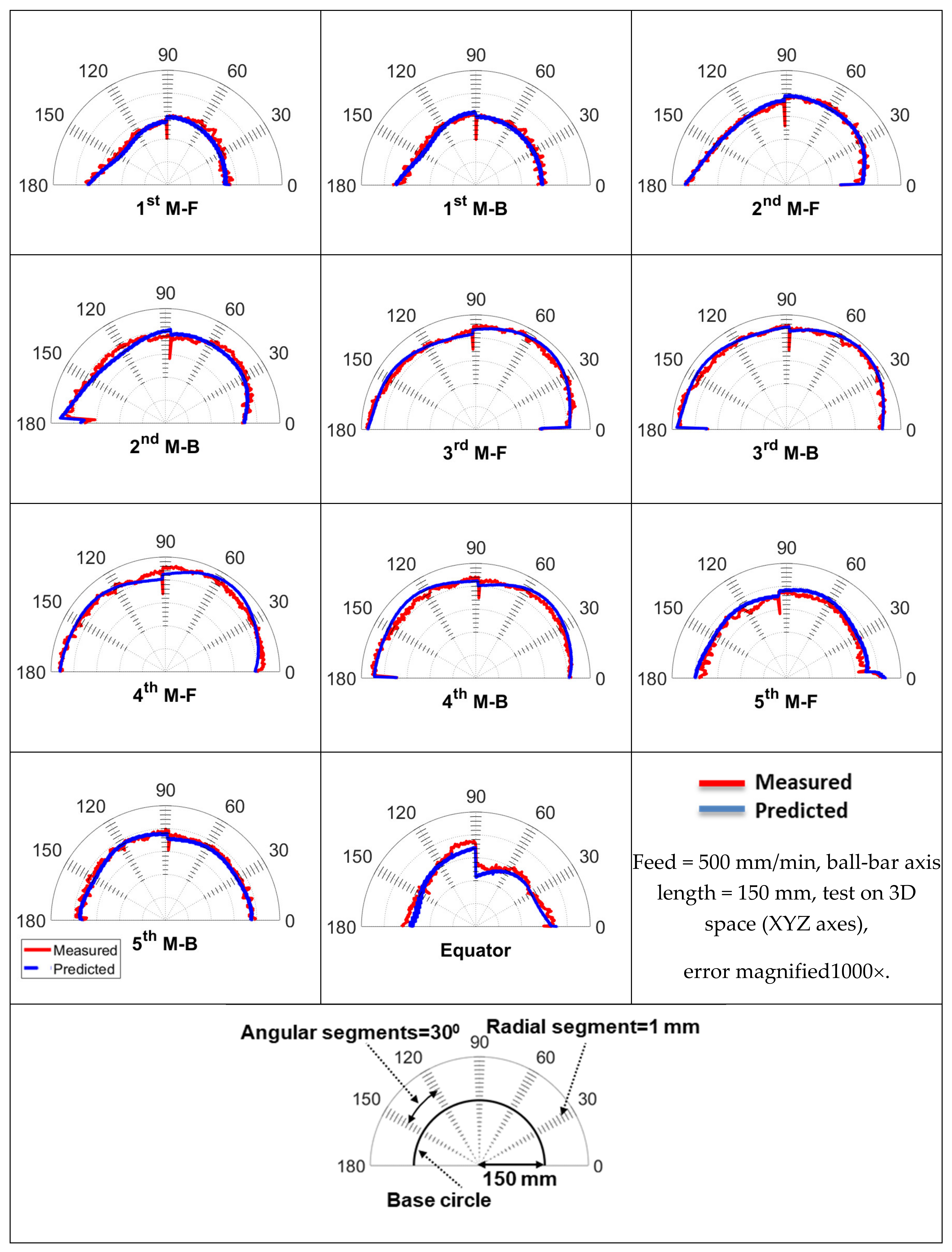
EZY2 (mm/mm2)	−6.47 × 10−7	1.81 × 10−7

lists the estimated error coefficients and their uncertainties. The predicted Cartesian volumetric errors calculated using the estimated coefficients in Equations (1) and (2) are projected in the sensitive ball-bar direction and compared with the experimental ball-bar measurements in Figure 5. The 10 polar plots show the forward and backward meridian travels. The model prediction closely matches the experimental data. As seen in Figure 5, the minimum errors are observed for the travel on the first meridian, which could be because only the X- and Z- axis errors are involved. However, for the rest, all the X-, Y-, and Z-axis errors are involved.

The maximum discrepancy between the predicted and the measured projected Cartesian volumetric errors is less than 2 µm. The maximum backlash happens for the Y-axis, EYYb, which is around −3 µm. However, the minimum backlash is for X-axis, EXXb, which a magnitude of 0.5 µm. The target machine tool does not reveal a big lateral play since the maximum lateral play is for the error coefficient EYXb with a magnitude of −0.4 µm. The backlashes and the lateral plays values are shown in Figure 6.

7. Conclusions

A geometric error model of a three-axis machine tool is proposed including all 18 intra-axis errors, the three out-of-squarenesses, and 18 hysteretic errors, one for each intra-axis error. Cubic polynomials enriched with hysteretic error terms capable of modeling backlashes and lateral plays are used yielding a total of 90 potential unknown error function coefficients. A minimal but complete set of the coefficient is selected using geometric reasoning as well as the sensitivity Jacobian column size, rank, and condition number. Considering a single tool length, if the three coordinates of the tool could be measured, a selection of 53 machine error coefficients could be estimated. In order to experimentally estimate these coefficients, various 2D and 3D ball-bar test strategies are simulated and their ability to estimate a maximum number of the necessary coefficients is analyzed using the sensitivity Jacobian. A five meridian plus the equator circle strategy is retained capable of estimating 37 error coefficients with a normalized Jacobian condition number of 1948. This strategy is tested on a five-axis machine tool and includes back and forth motions. The strategy analysis yields a maximum number of independent coefficients, which results in a good fit to the experimental data. The target machine tool reveals small backlashes. The model shows the maximum backlash for Y-axis for around −3 µm. However, the backlashes for X- and Z-axis are less than 1 µm. The proposed 3D ball-bar strategy predicts the projected Cartesian volumetric error where the maximum discrepancies between the prediction and the measurements are less than 2 µm. The simulations of different strategies showed that the 3D ball-bar strategy with one setup is able to distinguish a maximum of 37 machine error parameters.