Abstract
Refill Friction Stir Spot Welding (RFSSW) provides significant advantages over competing spot joining technologies, but detecting RFSSW’s often small and subtle defects remains challenging. In this study, kinematic feedback data from a RFSSW machine’s factory-installed sensors was used to successfully predict defect presence with 96% accuracy (F1 = 0.92) and preliminary multi-class defect diagnosis with 84% accuracy (F1 = 0.82). Thirty adverse treatments (e.g., contaminated coupons, worn tools, and incorrect material thickness) were carried out to create 300 potentially defective welds, plus control welds, which were then evaluated using profilometry, computed tomography (CT) scanning, cutting and polishing, and tensile testing. Various machine learning (ML) models were trained and compared on statistical features, with support vector machine (SVM) achieving top performance on final quality prediction (binary), random forest outperforming other models in classifying welds into six diagnosis categories (plus a control category) based on the adverse treatments. Key predictors linking process signals to defect formation were identified, such as minimum spindle torque during the plunge phase. In conclusion a framework is proposed to integrate these models into a manufacturing setting for low-cost, full-coverage evaluation of RFSSWs.
1. Introduction
1.1. Aluminum Joining Challenges and Refill Friction Stir Spot Welding (RFSSW) Emergence
Resistance spot welding (RSW) has dominated sheet metal joining for decades, with the average car containing 4000–6000 RSWs [1]. However, RSW suffers from several challenges when used on aluminum, including shortened electrode life due to inadvertent aluminum copper alloying [2,3,4], high energy consumption due to aluminum’s low electrical resistivity [4,5], and porosity due to molten aluminum’s hydrogen solubility (Figure 1b) [6]. As automotive and other industries transition from steel to aluminum to produce lighter, more efficient vehicles, there is a growing need for alternative joining technologies.
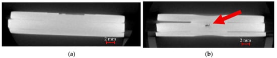
Figure 1.
Computed tomography (CT) scans of equivalent (a) refill friction stir spot weld (RFSSW) and (b) resistance spot weld (RSW) on a three-sheet stack-up of aluminum. The RSW exhibits a void [6]. Arrow added to highlight void location.
Self-piercing riveting (SPR), another widely adopted joining method, employs a semi-tubular rivet that pierces the top sheet and flares into the lower sheet, forming a mechanical interlock without fully penetrating the bottom sheet [4]. SPR offers rapid installation without pre-drilling or extensive surface preparation [4]. However, SPRs require an additional supply chain and feeding system due to the addition of the rivet, adding weight and complicating manufacturing. Moreover, SPR joints are also prone to stress concentrations, corrosion, fretting wear, and material thickness limitations [4,7].
Friction stir welding (FSW) is a unique joining technique patented in 1991 [8]. FSW joins materials by utilizing a rotating tool that plunges into the workpiece and traverses along the joint, stirring the metals together without melting them [9,10]. This yields welds with a refined microstructure, low heat input, and no fusion-related defects (Figure 1b) [10]. Another key advantage of FSW is its ability to join high-strength alloys with minimal heat-induced weakening, preserving their mechanical properties [9,10,11]. FSW also enables robust welds in “non-weldable” aluminum series (like 2xxx and 7xxx) [9] and even dissimilar metals [10], expanding design possibilities.
Following the success of FSW in several industries, friction stir spot welding (FSSW) technologies emerged starting in 1993 [12]. However, most left an undesirable “keyhole” in the material where the tool was retracted, as shown in Figure 2a [13,14]. Despite its keyhole drawback, FSSW began seeing real-world adoption in the early 2000s in Toyota Prius and Mazda RX-8 body structures, slashing equipment costs by 40% and energy consumption by 99% in the RX-8 application [15,16].
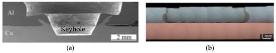
Figure 2.
Comparison of FSSW (a) and RFSSW (b) weld cross-sections. “Keyhole” label added and images rearranged [17]. Reproduced under the Creative Commons Attribution 4.0 International License (creativecommons.org/licenses/by/4.0).
In 1999, German researchers introduced RFSSW, a refinement of FSSW that employs a three-piece tool system to refill the undesirable keyhole [18]. This innovation leaves behind a relatively flush surface (Figure 2b) and produces a larger effective shear area than FSSW [18,19]. RFSSW inherits most of the advantages of FSW and FSSW, including solid-state joining without fusion defects [6,13,20,21]. Additionally, RFSSW eliminates common safety risks in RSW like expulsion and weld splash [22], while consuming just 2.5% of the energy required for an equivalent RSW joint [6]. Since its introduction, RFSSW has undergone extensive characterization [6,23,24,25], benefited from significant tooling advancements [26,27], and achieved weld times as short as 250 ms [28], enhancing its efficiency and industrial applicability.
1.2. RFSSW Theory of Operation
RFSSW employs a non-consumable three-piece tool with a clamp, shoulder, and probe, each capable of independent vertical movement. To create a weld, the non-rotating clamp first secures the sheets (Figure 3A). Then, the rotating shoulder plunges into the material while the rotating probe moves upward to accommodate displaced material (Figure 3B). Finally, the shoulder and probe return to the flush position (Figure 3C), and the clamp is retracted (Figure 3D) [20,21,29].
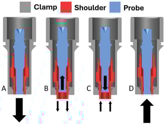
Figure 3.
A cross-section of a RFSSW tool during the four stages of RFSSW: (A) clamping, (B) plunging, (C) refilling, and (D) releasing.
1.3. RFSSW Defects
Like all joining methods, RFSSW is susceptible to defects. The sharp undercut at the top of Figure 4, labeled as “incomplete refill”, is a condition often caused by volume loss, insufficient flow, or lack of pressure during the refill stage [24,30]. Internal voids may also arise for similar reasons [13,24]. Defects shown below as “lack of mixing”, “partial bonding”, and “bonding ligament” are different forms of kissing bonds—areas of incomplete metallurgical bonding that diminish joint strength [13,14]. These kissing-type defects can be especially difficult to detect [31,32]. Similarly, a hook defect, where the gap between sheets is displaced downward or upward, can form a stress concentration despite minimal separation [11].
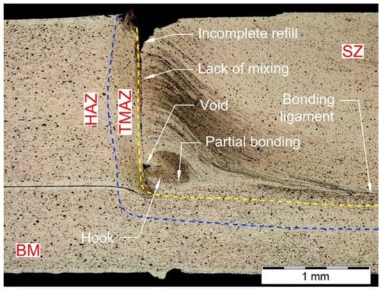
Figure 4.
Cross section of an RFSSW joint showing several defects [30]. SZ: stir zone, HAZ: heat affected zone, TMAZ: thermo-mechanically affected zone, BM: base material. Reproduced under the Creative Commons Attribution 4.0 International License (creativecommons.org/licenses/by/4.0).
These defects, often smaller than 0.1 mm, render traditional non-destructive testing (NDT) methods, such as ultrasonic testing (UT), less effective due to their limited resolution [32,33]. This detection challenge underscores the need for advanced techniques—like the machine learning approach proposed here—that combine the high sensitivity of costly destructive methods with the speed and affordability of NDT.
1.4. Conventional Weld Evaluation Methods
Destructive evaluation methods like cut-and-polish analysis and tensile testing are the gold standard for weld evaluation but often not practical to use in volume. Not only do they destroy the specimen, but they are also labor intensive. In contrast, non-destructive evaluation (NDE) methods evaluate welds without damaging the workpiece. There are a wide range of NDE methods, each with variable effectiveness in detecting defects, depending on the size, orientation, type, and material properties of the base metal [33].
Ultrasonic testing (UT) employs high-frequency sound waves to detect internal defects. It is widely used to measure nugget size [34], but struggles to reliably detect small voids, limited by the wavelength of an ultrasound wave [33,35]. One popular automation company’s UT system claims a resolution of only 0.35 mm [36]. This presents challenges for RFSSW’s smaller defects.
Thermography detects surface and sub-surface anomalies like expulsion or voids using infrared cameras, offering non-contact, real-time capabilities, but it struggles with deeper defects and with separation that is perpendicular to the sheet [35]. Eddy current testing identifies surface cracks quickly but is ineffective for deeper defects due to the skin effect, which becomes even more pronounced in highly conductive materials [37]. Radiographic testing (X-ray/CT) provides detailed internal imaging but is costly and poses radiation risks. Visual inspection is simple and low-cost but is limited to surface defects. Table 1 summarizes the minimum detectable crack sizes for different NDE methods, as reported by a NASA study [38], revealing detection limits approximately an order of magnitude larger than the ~0.1 mm defects illustrated in Figure 4.

Table 1.
NASA-STD-5009B Minimum detectable surface crack sizes for different NDE methods while requiring 90% probability of detection [38]. The data has been simplified by calculating some thickness-dependent values for a 3 mm-thick sheet to avoid having variables in the table.
Traditional NDE methods often suffer from limited resolution and depth, while destructive testing damages the workpiece and introduces additional processes, and both can be costly. The ML approach described herein utilizes kinematic data to enable efficient, low-cost, high-accuracy quality assessment for RFSSW.
1.5. Review and Research Gap
Existing ML research on metal joining quality falls into two main areas: those making predictions based on machine settings like RPM and dwell time as inputs, and those using process feedback as inputs, with machine settings held constant. Feedback-based prediction best supports established manufacturing and is the focus of this study.
Prior research has been conducted on self-piercing riveting (SPR) quality prediction. Ferrándiz, et al. [39] used force over displacement curves to predict SPR cross-sectional features like interlock distance using an autoencoder to encode the curves and a multilayer perceptron (MLP) to make the predictions, achieving a mean relative absolute error of 5.37 × 10⁻² mm on the cross-sectional features. Chen, et al. [40] utilized bidirectional long short-term memory (LSTM), a type of recurrent neural network, to predict defects binarily based on temporal variations in punch force during SPR, attaining a 94% F1 score. Oh, et al. [41] used scalar punch force data and a convolutional neural network (CNN) to predict SPR cross-sectional shapes, with a mean intersection-over-union of 98.50% and a mean pixel accuracy of 99.78%.
Prior research on RSW includes work by Zhou, et al. [42], who utilized dynamic electrical resistance curves to detect expulsion, a critical defect involving the ejection of molten metal from the weld nugget. By sampling resistance values every 1 ms, a 200-dimension vector was created, achieving 90–95% classification accuracy with several common models, on a moderately balanced production dataset of over 63,000 welds. Bogaerts, et al. [43] used an autoencoder feeding a gaussian process regression model to predict nugget diameter based on resistance curves, achieving better performance than a state-of-the-art geometry-based method. They used shims to create variations in resistance. Zhao, et al. used dynamic resistance curves to predict weld nugget diameter, achieving the highest predictive accuracy and robustness with a principal component analysis (PCA)-based linear regression model (R2 = 0.93 on training data, root mean square error (RMSE) = 0.12 mm) compared to a manual statistical feature-based linear regression model and an artificial neural network model. Chuenmee, Phothi, Chamniprasart, Khaengkarn, and Srisertpol [34] used statistical features such as mean, maximum, and total sum on weld pressure, current, and resistance to predict expulsion and cold welds. They compared five different models, and XGBoost (extreme gradient boosting) performed the best, achieving 93% precision and 98% recall. Notably, XGBoost outperformed more complex models such as the traditional neural network, LSTM, and CNN. This trend of simpler models outperforming more complex models was observed across multiple reviewed studies and may stem from complex models requiring larger training datasets and being more susceptible to overfitting.
For FSW, Hunt, et al. [44] demonstrated that force data could be processed with power spectral density (PSD), an alternative based on a Fast Fourier Transform (FFT), to classify full welds as defective or non-defective with 100% accuracy. Specific defect locations could be predicted with a 94% true positive rate (TPR) and a 4.2% false positive rate. Nadeau, et al. [45] compared K-nearest neighbors (KNN), MLP, support vector machine (SVM), and random forest algorithms for defect type and location detection based on averaged kinematic data. They reported that KNN yielded the best results, another instance in which simpler models beat much more complex models. Das, et al. [46] compared support vector regression, neural networks, and general regression to predict tensile strength based on wavelet transforms (a signal decomposition method) of force data from 65 welds. Support vector regression performed the best, followed by the neural network, with general regression having the worst performance. Other research shows feed-forward neural networks as a viable option for defect detection in FSW [47,48,49]. More complex neural network architectures such as convolutional neural networks [50] and recurrent neural networks [51,52,53,54] have also shown success.
It is important to note that while this previous work provides a foundation for RFSSW, the data collected in RFSSW differs from FSW. RFSSW yields only brief signal durations, with distinct stages. RFSSW also gives us different kinematic data than other joining methods, with spindle torque as well as force data from both the probe and the shoulder.
ML-based defect detection for RFSSW is less explored. Zhong, et al. [55] used laser scanning of surface topology of RFSSW and SVM to predict plug-type fracture versus all other types of tensile testing failure with 95.8% accuracy. Li, et al. [56] correlated features derived from three-dimensional ultrasonic scans of welds to shear strength, achieving a 0.89 correlation coefficient. Dahmene, et al. [57] used acoustic emission and a handful of classification algorithms (SVM, KNN, decision tree, discriminant analysis, and naïve bayes) to attempt binary classification (classes: defective, non-defective), as well as multi-category classification (classes: healthy, defective with flash, defective with lack of mixing, and defective with incomplete refill). Their dataset contained 48 samples. KNN was able to correctly identify 30 out of 34 defective welds, resulting in an 88% TPR, but this dataset was quite small. These studies, leveraging surface topology, ultrasonic, and acoustic emission data, demonstrate valuable approaches; however, using ML on RFSSW’s unique kinematic signals remains underexplored.
1.6. Research Objective
Leveraging kinematic feedback data to predict joint quality has been extensively explored in various joining techniques, yet its application to RFSSW remains underexamined. This paper addresses this gap by developing two ML models, with objectives including (1) constructing a binary classification model for final quality assessment and (2) developing a classification model to predict the original adverse treatment category (root cause), both illustrated in Figure 5.
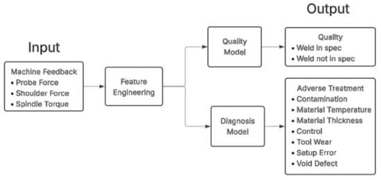
Figure 5.
Flowchart showing inputs and outputs of both models.
2. Materials and Methods
2.1. Machine, Tooling, and Materials
Welds were performed at Brigham Young University’s Friction Stir Research Laboratory using a Bond RS2 RFSSW robotic (Bond Technologies, Inc., Elkhart, IN, USA) end effector (Figure 6). The system records kinematic data from the clamp, shoulder, and probe. In the setup, data was output at 654 Hz. The machine has a maximum spindle speed of 6000 rpm, a maximum torque of 23 Nm, and a throat depth of 609 mm (24 in). A small fixture table with pins and holes was added to the anvil area to allow coupons to be aligned and clamped into position (Figure 6).
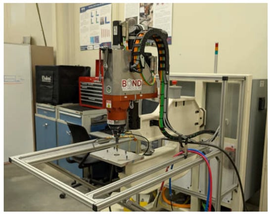
Figure 6.
Bond RS2 RFSSW machine used in this study, with fixturing table.
The toolset consisted of a W360 tool steel probe (Bond P.N. D11853), a 7 mm OD shoulder (Bond P.N. D11852), and an H13 tool steel clamp (Bond P.N. D11851). The probe and shoulder were coated with diamond-like-carbon, while the clamp was coated with Ti-carbide di-sulfide.
All welds in this study were performed on AA6061-T4 aluminum, with the composition shown in Table 2. The material was older than 90 days, aging it out of a true T4 state.
Table 2.
Chemical composition of AA6061-T4 by weight.
Coupons measured 100 mm × 30 mm. The top coupon was 2.4 mm thick, and the bottom coupon was 1.2 mm thick. For each treatment, ten welds were conducted across four stack-ups to support varied testing (Figure 7): three welds on three stack-ups of fully overlapped coupons (Figure 8) for CT scanning, cross-sectional analysis, and profilometric measurements, and one weld on partially overlapped coupons (Figure 9) for tensile testing.
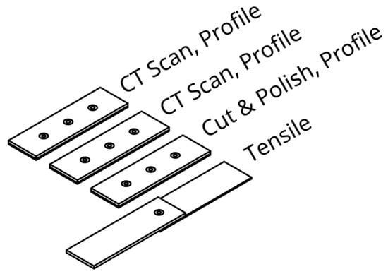
Figure 7.
A diagram showing the ten welds performed for every treatment, including the coupon configurations, and the testing methods for each of the four coupons.
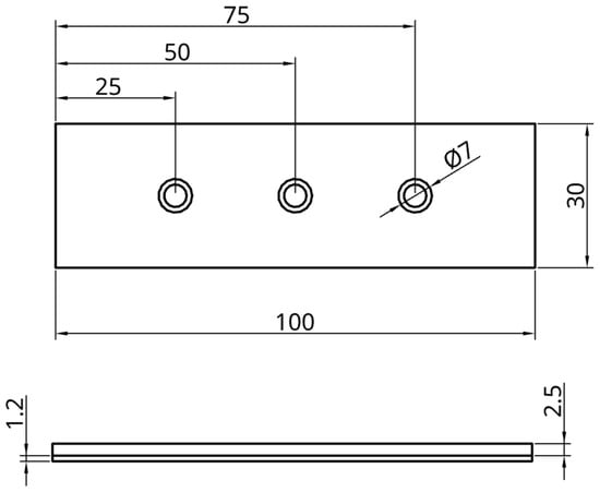
Figure 8.
A drawing depicting a top and side view of the non-tensile test coupon configuration.
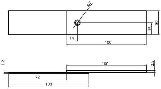
Figure 9.
A drawing depicting a top and side view of the tensile test coupon configuration.
2.2. Welding Procedure
2.2.1. Default Welding Procedure
All welds were 7 mm in diameter, produced at 2500 RPM spindle speed, with a 3.0 mm plunge depth, and 1000 ms total weld time. Machine parameters remained constant across all treatments. These parameters and general setup were validated in a previous study to produce good welds [6].
Tools were cleaned with NaOH before beginning the experiment. Coupons were wiped with 90% isopropyl alcohol (IPA) prior to welding. Spindle liquid cooling was utilized. Three warm-up welds were performed from a cold start to enhance consistency. A post-weld mechanical cleaning cycle was performed after each weld, which included five up-and-down movements of the probe within the shoulder, supplemented by 10 s of compressed air with a manual blow gun to remove debris and cool the tool. Welds were performed in a computer-generated randomized order with some exceptions. Treatments requiring excessive changeover time like those involving contamination and worn tools were performed sequentially, only randomizing the ten coupon locations.
2.2.2. Adverse Treatments
Thirty treatments were performed to simulate issues that might cause defects in a manufacturing setting, such as drilling holes in certain places to induce volume loss (Figure 10a) or contaminating areas with anti-seize (Figure 10b). Ten welds per treatment resulted in a total of 300 treated welds. Treatments and details can be found in Table 3.
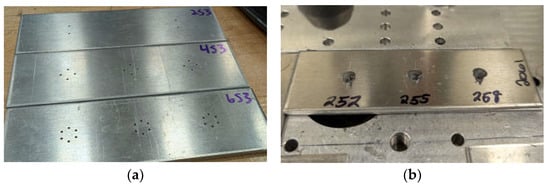
Figure 10.
(a) Coupons prepared for “void under shoulder” treatments by drilling 2, 4, and 6 holes under the shoulder. (b) Anti-seize on coupon for contamination treatment.
Table 3.
Adverse treatments.
2.3. Weld Evaluation
Testing protocols were adapted based on the varying resource demands of different methods. For each treatment, 9 profile measurements, 6 CT scans, 3 cut-and-polish images, and 1 tensile test (Figure 7) were performed.
2.3.1. Computed Tomography (CT) Scanning
Three-dimensional CT scans were performed with a Rigaku RmCT2 CT Scanner (Rigaku Corporation, Austin, TX, USA). Up to six coupons were scanned at a time. The scan time was 4 min, performed in high resolution at a 90 kV voltage, an 88 μA current, and a 72 μm voxel size. Scans were manually reviewed in 3 dimensions for consolidation within the weld and labeled accordingly (Figure 11).
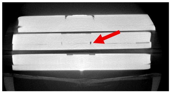
Figure 11.
CT scan of three welds, revealing a tunnel defect in the middle weld (red arrow). The treatment for this weld (weld #241) was “Contaminant between materials”.
2.3.2. Cut & Polish
Coupons were cut in the 30 mm direction (parallel to the 30 mm coupon edge), mounted in Bakelite, polished from 400 grit to 1200 fine grit, and imaged with a Keyence VHX-7000 Microscope (Keyence Corporation, Itasca, IL, USA) at 100× magnification with coaxial lighting. Results were manually reviewed for consolidation within the weld and labeled accordingly (Figure 12).
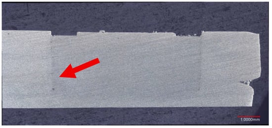
Figure 12.
Cut-and-polish image revealing a small tunnel void (red arrow). The treatment for this weld (weld #6) was “Weld close to an edge (2 mm)”.
2.3.3. Profilometry
Profile measurements were taken on the top surface of welds with a Keyence VHX-7000 profilometer. Included software was used to automatically align and crop the welds and find the deepest point on a cross-sectional view, yielding an undercut measurement (Figure 13).
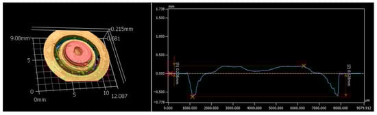
Figure 13.
Profilometry showing excessive undercut. Exaggerated 3D profile (left); cross-sectional profile graph, with blue line indicating the profile, and the vertical red lines indicating max depth and height measurements (right). The treatment for this weld (weld #252) was “Contaminant on top”.
2.3.4. Tensile Testing
Quasi-static tensile testing was performed using an Instron 4204 Tensile Tester (Instron, Norwood, MA, USA), with samples subjected to a pull rate of 10 mm/min. Spacer coupons were placed in the tensile tester jaws to ensure tensile force was parallel to weld interface. The ultimate tensile strength (UTS) and total energy absorption (TEA) were captured. The failure mode was also recorded as “bottom sheet nugget pullout”, “top sheet nugget pullout”, or “interfacial” (Figure 14). Interfacial failure is undesirable because it indicates complete and sudden failure of the weld, with potentially brittle characteristics.
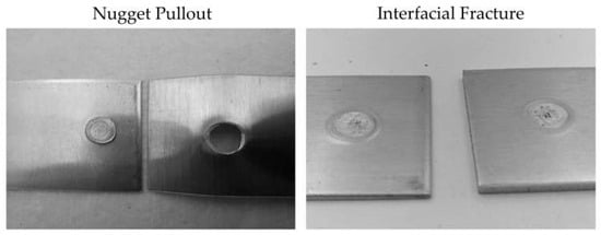
Figure 14.
Tensile failure modes: (left) nugget pullout; (right) interfacial fracture [6].
2.4. Data Preparation
2.4.1. Feature Extraction
The three signals in Table 4 were selected as ML features. Position and velocity signals were not used as features since the machine runs in position control mode.
Table 4.
Feedback signals selected for use as model input.
Data processing was conducted using a custom Python 3.14 class, which consolidated data from three sources: time-series CSV files containing machine output, an Excel file from the profilometer (for undercut), and a manually curated CSV file documenting tensile testing, cut-and-polish inspections, and CT scan results. Time-series signals were aligned and cropped to a 1.5-s window centered on the minimum shoulder position (Figure 15).
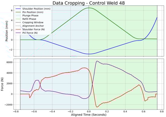
Figure 15.
Plot of tool position and forces over time, with background showing cropping window (dotted lines), as well as plunge (light blue) and refill (light green) phases.
Following cropping, FFT spectral diagrams of probe force, shoulder force, and spindle torque were visualized and explored briefly. Although the signals may not align well with FFT’s stationarity and periodicity prerequisites, this evaluation was conducted as an exploratory analysis to assess potential frequency-based insights. If spectra indicated predominantly low frequencies, it would suggest the data is dominated by slow-varying trends rather than periodic oscillations, suggesting limited suitability for traditional FFT. Based on this assessment, the authors opted not to pursue FFT further and shifted focus to statistical feature extraction.
Time-series signals were segmented into three distinct phases: whole-signal, plunge, and refill (Figure 15). For each phase and signal, a comprehensive set of statistical features were extracted, including mean, standard deviation, skewness, kurtosis, entropy, root mean square (RMS), maximum, minimum, integral, peak-to-peak amplitude, and the timestamps of maximum and minimum values. Formulae for these features are given in Table A1. Derivative features were computed using a three-point central difference method to highlight dynamic variations, followed by vectorization with the aforementioned statistical features, excluding mean (which would be zero due to the derivative’s properties) and integral (as it approximates the original signal) (Figure 16). Integral features were computed using Simpson’s rule. Additionally, an area difference feature was obtained by integrating the difference between shoulder and probe forces over time. This broad feature set of 228 features was intentionally developed to facilitate future evaluation of dimension reduction strategies.
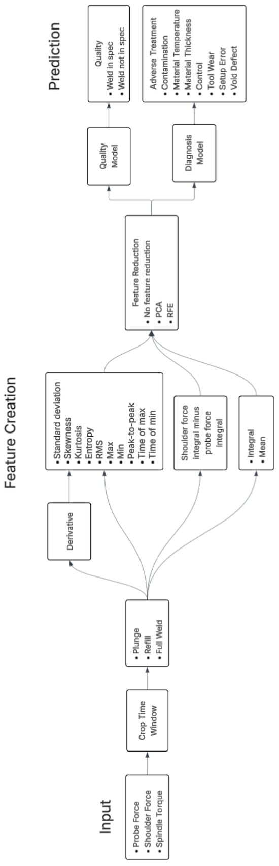
Figure 16.
Flowchart showing feature creation methodology.
2.4.2. Diagnosis Label Creation (Multi-Class)
The 30 unique adverse treatments were condensed into the seven key categories presented in Figure 17 to simplify the classification task and allow for more training data per category. Predicting many individual conditions is difficult with limited data, and many of the adverse treatments were similar to each other.
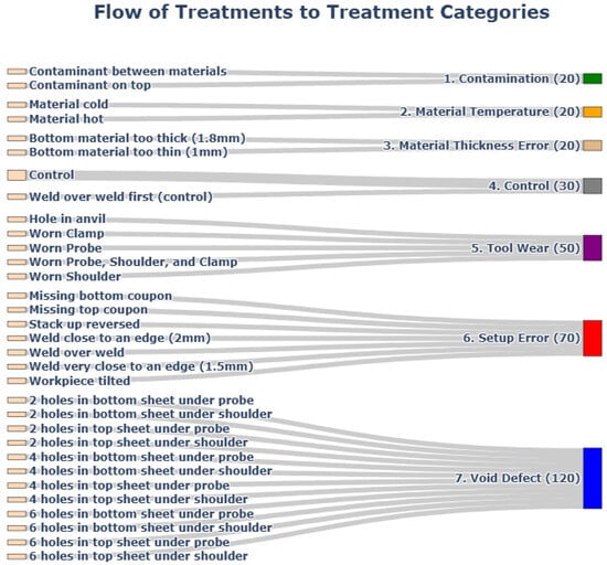
Figure 17.
Flowchart showing the treatment consolidation strategy.
To mitigate data scarcity within the control group, the dataset was augmented with the initial 10 welds that were prepared for the ‘Weld over weld’ condition. While these specific samples were not subjected to destructive post-mortem inspection, internal process qualification studies using this specific RFSSW configuration have yielded over 5000 consecutive defect-free welds (unpublished results). Given this exceptional statistical reliability, the probability of latent defects within these initial welds is negligible, justifying their inclusion alongside the 20 other tested controls.
2.4.3. Quality Label Creation (Binary)
To create binary labels (‘pass’ or ‘fail’) for weld quality, specific criteria were established for each test. These thresholds were deliberately more stringent than typical industrial specifications to aid model training and fight dataset imbalance. For UTS and TEA, the lowest 25% of tested welds (not including controls) were labeled ‘fail’ due to the relatively high values across the dataset, prioritizing sensitivity to subtle quality differences. This 25% cutoff point ended up being 4820 N for UTS and 8 J for TEA. For CT scans and cut-and-polish inspections, welds were manually reviewed, with any visible voids or lack of consolidation resulting in a ‘fail’ label. For tensile failure mode, one weld exhibiting interfacial failure—associated with contamination between materials—was labeled ‘fail’, while all others, showing nugget pullout, were labeled ‘pass’. Profilometry measurements followed existing literature, failing welds with undercut ≥0.2 mm [11,58]. The ‘final pass/fail’ label, which served as the model prediction goal, was assigned ‘fail’ if a weld failed any conducted test (Figure 18). All welds with the missing top or bottom coupon treatment were automatically failed since no joint was created. A sanity check confirmed that all control welds passed all performed tests. This resulted in 222 welds labeled ‘pass’ and 108 labeled ‘fail’ for the ‘final pass/fail’ category, providing a dataset with an acceptable amount of imbalance (Figure 19).
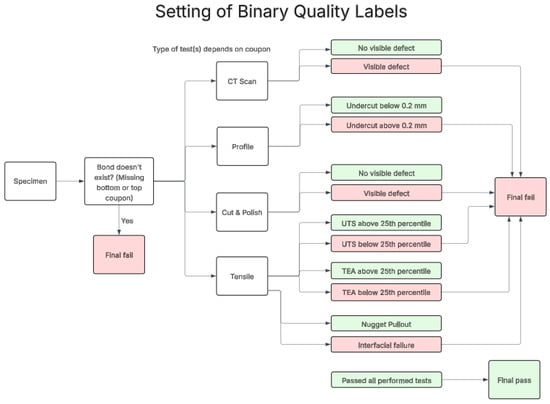
Figure 18.
Flowchart showing the logic used to create binary labels. Red boxes indicate failing states while green boxes indicate passing states.
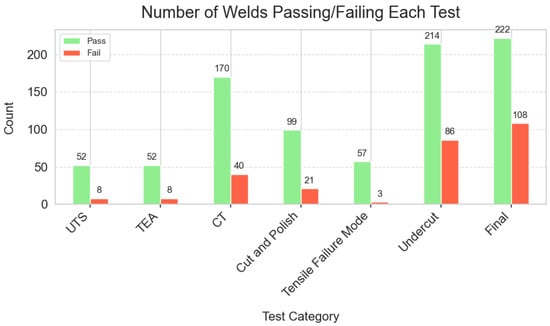
Figure 19.
Bar chart showing the number of welds that passed and failed each test. The 30 control welds are included in each of the passing counts, so counts comprise of welds evaluated via that method plus the 30 controls.
The adoption of a heterogeneous validation strategy, wherein different testing methods (e.g., tensile testing, CT scanning, profilometry) were applied across the dataset, inherently introduces label variability regarding the definition of failure. While this variability can make the optimization landscape more complex—as a specific sample might pass a less-sensitive test (e.g., tensile) despite containing defects that would be caught by a stricter method (e.g., CT)—it forces the model to learn a more generalized and robust representation of quality. By aggregating diverse validation metrics, the effective ground truth reflects a composite of failure modes (encompassing internal, surface, and mechanical defects) rather than relying on a single, potentially narrow proxy for integrity. Consequently, the model learns to identify the kinematic signatures of defects regardless of which specific test was used to validate them. In this context, a ‘False Positive’ (predicting failure on a physically passing weld) often indicates that the model detected a latent defect that the assigned testing method missed. This robustness is evidenced by the model’s high classification accuracy, which confirms it successfully filtered out method-based label noise to discern failure. Furthermore, because validation methods were assigned randomly rather than being correlated with specific defect types, the model is prevented from overfitting to the biases of any single testing modality.
2.5. Model Development
2.5.1. Models
Distinct models were developed for the two tasks using the same development and training pipeline. Five classifiers were compared: logistic regression, a linear model effective for binary and multi-class problems with interpretable coefficients; random forest, an ensemble method that leverages multiple decision trees; SVM, a distance-maximizing algorithm that identifies the optimal boundary to separate classes; MLP, a simple neural network capable of capturing complex patterns through multiple layers; and XGBoost, another ensemble method that integrates many basic decision trees.
Most models were instantiated using the scikit-learn python package with default settings (except SVM, where probability = true was enabled to generate probabilities and support precision recall curves). XGBoost was sourced from the XGBoost package for its optimized gradient boosting and early stopping capabilities.
For each task, numerical features were standardized using StandardScaler from scikit-learn, which transforms features to have a mean of 0 and a standard deviation of 1. This standardization ensures that features with different scales contribute equally to model training, improving convergence for distance-based models like SVM and gradient-based models like neural net. Categorical labels were encoded using scikit-learn’s LabelEncoder for the multi-class model.
2.5.2. Evaluation
The performance was evaluated based on F1 scores (Equation (1)), which represent the harmonic mean of precision (Equation (1)) and recall (Equation (2)).
The F1 metric effectively balances the accurate identification of minority classes—such as ‘fail’ or less common issue types—with the reduction of false positives, making it well-suited for imbalanced datasets. For the multi-class problem, the scikit-learn average = ‘macro’ setting was applied, which assigned equal weight to each class’s score irrespective of its size. This approach can enhance the visibility of smaller classes’ performance, but it may also lower the overall F1 if minority classes are poorly predicted, reflecting the true challenge of dataset imbalance.
The dataset was split into training (85%) and test (15%) sets using scikit-learn’s train_test_split function. For the multi-class task, stratification was applied across the output to preserve the class distribution across sets. For the binary task, a random (non-stratified) split was used, as the classes were larger (222 Pass, 108 Fail). No data leakage occurred, as verified by explicit checks confirming zero index overlap between training and test sets. The held-out test set was reserved exclusively for final model evaluation. During development, models were compared with 5-fold stratified cross-validation on the training set, optimizing for the F1 score. Cross-validation is a technique that splits the training data into, in this case, five parts, trains the model on four parts, and tests it on the remaining one. It continues to rotate through parts, then takes the average of the five results to get an overall performance score. Cross-validation was employed during model development, with the test data reserved for the final assessment. Reserving a test set for use only at the final evaluation stage is a best practice that helps prevent overfitting to the test data.
2.5.3. Dimension Reduction
Dimension reduction can improve model performance by removing noise and redundant features, reducing computational complexity and preventing overfitting. With the extensive feature set generated, two different dimension reduction strategies were evaluated: recursive feature elimination (RFE), a method that iteratively removes the least-important features based on model performance, PCA, a technique that transforms the original features into a new set of uncorrelated principal components, and no reduction. For RFE, tests were performed retaining 10, 30, 50, and 100 original features. For PCA, 95% of the variance of the original data was retained.
2.5.4. Hyperparameter Tuning
Model hyperparameters were tuned using grid search over predefined parameter grids. Scikit-learn’s GridSearchCV was employed to exhaustively evaluate all combinations in the specified grids for each model, optimizing the F1 score through 5-fold stratified cross-validation. The tested parameter grids are shown in Table 5.
Table 5.
Possible parameter values for tuning models.
2.5.5. Post-Development Model Analysis and Final Model Selection
Final model selection was driven primarily by macro F1 score on the held-out test set (15% of the data). The model with the highest F1 score was chosen so long as there was not a significant drop between the validation F1 score and the hold-out F1 score, which would indicate overfitting.
After determining the best root cause and quality models, they were analyzed for robustness and interpretability. SHAP (SHapley Additive exPlanations) was utilized to assess the contribution of each feature to the predictions, revealing the most influential variables. Feature importance was also calculated with a decision tree to compare with SHAP. Ablation studies were performed to evaluate the significance of the plunge versus refill stages, as well as the relative importance of shoulder force, probe force, and spindle torque. Visualizations such as confusion matrices and precision–recall curves were generated. Additionally, instances of incorrect model predictions were analyzed.
3. Results
3.1. Fast Fourier Transform (FFT) Results
Visualization of FFT spectra (Figure 20) revealed a dominance of low-frequency components, with no prominent frequency peaks. Notably, even the expected rotational frequency of the tool (2500 RPM/60 = 41.67 Hz) was not readily visible in the spectra of shoulder force, probe force, or spindle torque.
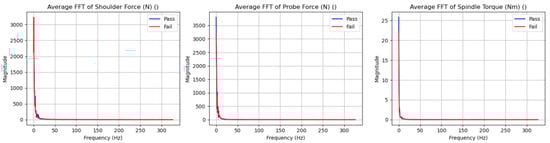
Figure 20.
FFT spectra of shoulder force, probe force, and spindle torque.
The authors theorize that this absence of a clear rotational signature is attributable to the inherent symmetry of the refill friction stir spot welding (RFSSW) process. Unlike linear friction stir welding (FSW), where tool imperfections or asymmetries can produce periodic torque/force variations as they repeatedly rotate towards and away from the advancing side of the weld, the plunged RFSSW tool experiences radially symmetric material flow around its axis. This symmetry results in more consistent frictional conditions throughout each rotation, yielding negligible torque or force fluctuations tied to the spindle rotation frequency.
Potential data acquisition issues, such as aliasing or excessive filtering, were ruled out: The 654 Hz sampling rate provides a Nyquist frequency of 327 Hz, well above the 41.67 Hz rotational frequency, ensuring adequate capture of any periodic component at that frequency.
This FFT test was conducted as part of exploratory data analysis. Once time-domain statistical features demonstrated higher feasibility, frequency-domain approaches were not pursued further.
3.2. Baseline Models
Baseline models were scored to provide a foundation for subsequent optimization. All binary models achieved F1 scores exceeding 0.9 (Figure 21a), while multi-class models recorded scores ranging from 0.599 to 0.762 (Figure 21b). As noted previously, the use of equal weighting for the F1 score across all classes, including smaller ones, likely contributes to the lower multi-class scores. Nevertheless, the baseline multi-class models still demonstrated meaningful predictability, as a random model predicting across seven classes would yield an F1 score and accuracy of only 1/7 ≈ 0.14.
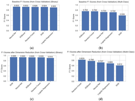
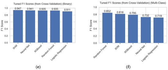
Figure 21.
F1 scores at different pipeline stages including the baseline (a) quality/binary and (b) diagnosis/multi-class scores, scores after dimension reduction (c,d), and scores after parameter tuning (e,f).
3.3. Dimension Reduction
Prior to dimension reduction, the models were processing 228 features per weld. RFE successfully reduced this to 30 features for both models (Figure 22) while increasing F1 scores (Figure 21c,d). This elimination of ~85% of the features simplifies the models and lowers their complexity. PCA generated 25 features, retaining 95% of the variance, yet underperformed compared to RFE. Moreover, RFE maintains feature interpretability, unlike PCA, whose features are abstract. The highest-performing models for each task were used to compare the dimension reduction techniques, Neural Net for quality, and XGBoost for diagnosis, followed by the re-testing of all models (Figure 21c,d). This re-testing yielded an F1 score improvement of 0.013 for the leading binary classification model and of 0.067 for the multi-class model.
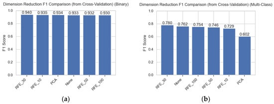
Figure 22.
Comparison of F1 scores across different dimension reduction techniques on (a) quality/binary model and (b) diagnosis/multi-class.
3.4. Hyperparameter Tuning
Model parameter tuning boosted the performance of the multi-class models (Figure 21f) but had limited impact on the binary models (Figure 21e). Across the improved models, enhancements largely resulted from changing parameters that governed model complexity (Table 6). For example, SVM’s dramatic rise from fourth place to first place came after increasing its C factor, an action that reduces regularization. Regularization is a factor that penalizes model complexity to prevent overfitting. Reducing this penalty allowed a tighter fit to the training data, which likely addressed the seven-class challenge more effectively.
Table 6.
Parameter sets and F1 scores before and after hyperparameter tuning for multi-class model.
3.5. Results for Top Performing Models
3.5.1. Binary Quality Model
Support vector machine exhibited the highest F1 score for predicting in-spec welds, with an accuracy of 96%, recall of 1.0, and F1 score of 0.92. Performance did not drop when moving from the validation scoring to the test set scoring, indicating good performance on never-before-seen data. Two incorrect predictions were made on the test set. (Figure 23a). The model did not make any type II errors. Figure 23b shows a healthy precision–recall curve, indicating that the model could be tuned to be more sensitive by allowing for a limited number of false positives.
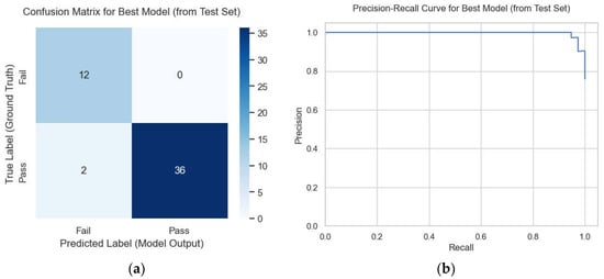
Figure 23.
Confusion matrix (a) and precision–recall curve (b) for top binary/quality model.
Among the 30 adverse conditions (plus control), 5 exhibited a 100% failure rate, 12 a 100% pass rate, and the remaining 15 showed variable outcomes (Figure 24). The model’s high performance, even on these 15 inconsistent conditions, demonstrates a nuanced understanding beyond mere treatment recognition, enabling discrimination between viable and defective welds even among the same treatment.
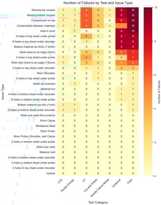
Figure 24.
Number of test failures for each test type by treatment.
The two misclassifications (Figure 23a) arose from these “grey area” treatments. Weld 415, subjected to the “6 holes in top sheet under shoulder” condition, passed tensile testing despite its treatment group having a 90% overall failure rate. The model’s failure prediction reflects this risk. While the mixed testing strategy may have contributed to this discrepancy, it promotes model generalization by capturing defect severity gradients. Similarly, weld 197, under the “weld very close to an edge (1.5 mm)” treatment, passed its assigned profilometry and CT scan, but the treatment group as a whole yielded 60% defects (Figure 24). These instances, although highlighting the challenges of stochastic defects, do seem to show that the model is tuned to both low-level process signals and higher-order patterns.
3.5.2. Multi-Class Diagnosis Model
After tuning, the highest-performing diagnosis model was random forest, with an accuracy of 84%, recall of 0.84, and F1 score of 0.82. The F1 score did not drop significantly when moving from the validation scoring to the test set scoring, indicating good performance on never-before-seen data.
Among the three setup errors the model overlooked (Figure 25), one resulted from a “stack-up reversed” treatment, and the other two from “weld over weld” conditions. These cases typically entail minimal material loss or base metal alterations—challenges that were anticipated would test the model’s limits. The model also misclassified two control welds as setup errors, presumably also owing to the same subtle overlaps between control samples and certain setup error treatments.
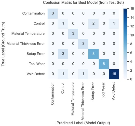
Figure 25.
Confusion matrix for top multi-class/diagnosis model.
3.6. Ablation Study
The ablation study revealed distinct differences in the importance of various signals, providing insights into their contributions to model performance. Among spindle torque, shoulder force, and probe force, all three enhanced the model’s predictive power, with spindle torque emerging as the most critical (Figure 26a). The authors hypothesize that torque’s prominence stems from its reflection of the substantial rotational work performed during welding, which likely offers a higher-fidelity and more informative perspective on the weld’s mechanical dynamics compared to the limited work of plunging such a short distance into the material. Shoulder force proved slightly more influential than probe force, likely due to its larger surface area and role in stirring the weld’s outer edges, a key factor in ensuring robust nugget formation.
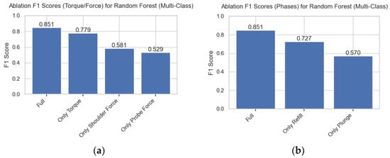
Figure 26.
F1 scores after ablating groups of torque/force features (a) and phases (b). Higher values indicate higher feature importance.
Furthermore, the relative importance of signals captured during the refill and plunge stages (Figure 26b) were evaluated, both of which played a substantial role in achieving the final model performance. However, refill signals emerged as particularly critical compared to those from the plunge stage. This heightened significance may stem from the forces at the weld’s conclusion, which provide a crucial indicator of any volume loss. Given that many of the induced issues in the dataset were related to material volume, this finding highlights the refill stage’s pivotal role in detecting such defects.
3.7. Feature Importance
Both SHAP (Figure 27) and feature importance derived from the random forest (Figure A1) showed similar results, identifying the minimum spindle torque during the plunge phase as the most critical feature to identify adverse treatments. The SHAP analysis further revealed that this minimum torque is a key predictor for both void formation and extreme material temperatures (Figure 27). Similarly, both algorithms ranked the skew of the torque curve during refill—a measure of the distribution’s asymmetry—as the second most influential feature. According to SHAP, torque refill skew had an especially large impact in identifying tool wear. Trained models, even those thought of as being “black boxes” can yield interpretable insights when paired with tools like SHAP.
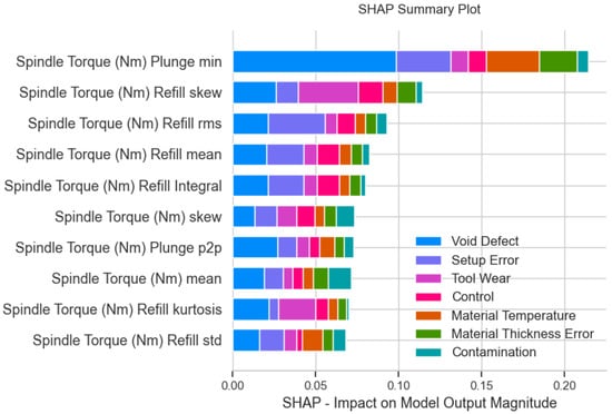
Figure 27.
Top 10 most impactful features (out of 228) for predicting the consolidated issue type, ranked by mean SHAP value.
3.8. Proposed Framework
In automotive body-in-white manufacturing, quality assurance often relies on visual inspection and manually performing UT on a sample of welds every shift, requiring a dedicated NDE team and equipment [34]. The in situ ML models developed in this study could allow for low-cost, 100% process evaluation with instant feedback, dramatically reducing the need for routine destructive or time-consuming NDE.
By using the regression versions of the classifiers, each weld can be assigned a continuous risk score. A threshold can be set so that only the highest-risk welds are selected for targeted destructive or advanced NDE verification. Since kinematic data are captured for every production weld, each manual verification instantly adds a new labeled example for training. These data are stored and periodically used to retrain the models in a semi-supervised, human-in-the-loop cycle. This approach provides a pathway to expand from limited data to a production-ready dataset, which will naturally include genuine material variation, tool wear progression, and process disturbances.
As performance improves, the verification rate can be reduced and the risk threshold adjusted to prioritize Type I or Type II errors as required. The risk score itself can be treated as a standard process variable, displayed on existing HMIs, and monitored with conventional SPC software, ensuring straightforward integration into production environments.
Transfer learning can facilitate the introduction of new alloys or weld parameters. A model trained on a mix of existing datasets could be fine-tuned using the first 100–200 RFSSW welds of a new setup.
4. Conclusions
In conclusion, this study demonstrates the feasibility of using factory-installed kinematic sensors and machine learning for in situ quality assessment and defect diagnosis in RFSSW, achieving 96% accuracy in binary pass/fail prediction and preliminary multi-class diagnostic capability. Key predictive features, such as minimum spindle torque during the plunge phase, provide valuable physical insights into defect formation mechanisms. The results are subject to limitations: The dataset is relatively modest (330 welds), the defects were artificially induced, and the multi-class evaluation suffers from low per-class test samples. Future work should focus on larger-scale industrial datasets with naturally occurring defects verified by comprehensive NDE, real-time model deployment, adaptive thresholding for varying setups, and semi-supervised human-in-the-loop strategies—such as selectively retesting welds that pass traditional evaluation but are flagged as problematic by the model.
Key Findings:
- High Predictive Accuracy: SVM excelled in binary quality assessment (F1 = 0.92), predicting with high accuracy, even for treatments that produced a mix of passing and failing welds.
- Preliminary Root-Cause Diagnosis Feasibility: Random forest led multi-class performance (F1 = 0.82), with misclassifications tied to subtle setup errors (e.g., “stack-up reversed”). These multi-class results are preliminary due to the limited test set size (n = 47) and low samples per class (as low as n = 3), and should be validated on larger, industrially sourced datasets.
- Feature and Signal Insights: SHAP and random forest analyses pinpointed minimum plunge torque as the top predictor for voids and temperature extremes, while ablation showed spindle torque to be more predictive than shoulder/probe force and refill signals to be more predictive than plunge forces.
- Dimensional Efficiency: RFE yielded minor F1 gains and an 85% reduction in input size.
- Accessible Baselines: Even undeveloped models delivered reasonable performance (F1 > 0.9 binary; F1 > 0.6 multi-class), suggesting the possibility of plug-and-play deployment without advanced ML expertise; however, tuning does offer further refinement.
- Framework for manufacturing integration: Probabilistic outputs can prioritize high-risk welds for targeted NDE (e.g., CT or tensile testing), reducing reliance on costly, low-coverage methods while enabling 100% inline evaluation. As production data accumulates, semi-supervised retraining could further refine performance. Numerical model outputs can be treated like SPC data and used in existing SPC software.
- Limitations include dataset scale (330 welds) and induced treatments’ focus on simulated defects, potentially limiting generalizability. Future work should expand to thresholding techniques for different setups, real-time deployment, and semi-supervised human-in-the-loop training—such as retesting welds that initially passed evaluation, but the model deemed problematic.
Author Contributions
Conceptualization, J.A. and Y.H.; methodology, J.A., Y.H., T.S. and J.J.; software, J.A.; validation, J.A.; formal analysis, J.A.; investigation, T.S., J.J., J.M. and J.A.; resources, J.A.; data curation, J.A.; writing—original draft preparation, J.A.; writing—review and editing, J.A., Y.H., T.S. and J.J.; visualization, J.A.; supervision, Y.H.; project administration, Y.H.; funding acquisition, Y.H. All authors have read and agreed to the published version of the manuscript.
Funding
This research was funded by Toyota Motors North America through the National Science Foundation IUCRC—Center for Friction Stir Processing (CFSP) under Brigham Young University Friction Stir Research Lab account GR00277.
Data Availability Statement
The data presented in this study is available on request from the corresponding author. The data sets are not publicly available due to their complex structure.
Acknowledgments
We acknowledge the Brigham Young University MRI Facility for providing CT scanner access and expertise. ChatGPT-5 was used to improve code structure and syntax. The authors have reviewed and edited the output and take full responsibility for the content of this publication.
Conflicts of Interest
The authors declare no conflicts of interest. The funders had no role in the design of the study; in the collection, analyses, or interpretation of data; in the writing of the manuscript; or in the decision to publish the results.
Abbreviations
The following abbreviations are used in this manuscript:
| BM | Base Material |
| CNN | Convolutional Neural Network |
| CFSP | Center for Friction Stir Processing |
| CT | Computed Tomography |
| FFT | Fast Fourier Transform |
| FSSW | Friction Stir Spot Welding |
| FSW | Friction Stir Welding |
| HMI | Human-Machine Interface |
| IPA | Isopropyl Alcohol |
| KNN | K-Nearest Neighbors |
| LSTM | Long Short-Term Memory |
| ML | Machine Learning |
| MLP | Multilayer Perceptron |
| NDE | Non-Destructive Evaluation |
| NDT | Non-Destructive Testing |
| PCA | Principal Component Analysis |
| PSD | Power Spectral Density |
| RFE | Recursive Feature Elimination |
| RFSSW | Refill Friction Stir Spot Welding |
| RMS | Root Mean Square |
| RMSE | Root Mean Square Error |
| RSW | Resistance Spot Welding |
| SHAP | SHapley Additive exPlanations |
| SPC | Statistical Process Control |
| SPR | Self-Piercing Riveting |
| SVM | Support Vector Machine |
| TEA | Total Energy Absorption |
| TMAZ | Thermo-Mechanically Affected Zone |
| TPR | True Positive Rate |
| UT | Ultrasonic Testing |
| UTS | Ultimate Tensile Strength |
| XGBoost | Extreme Gradient Boosting |
Appendix A
Table A1.
Formulae for statistical features.
Table A1.
Formulae for statistical features.
| Feature | Formula | Notes |
|---|---|---|
| Mean | ||
| Standard Deviation | ||
| Skew | Measures if distribution leans left or right. | |
| Kurtosis | Measures how peaked or flat a data distribution is, indicating tail heaviness. | |
| Entropy | Quantifies the randomness or uncertainty in a data distribution. | |
| Root Mean Square (RMS) | Calculates the square root of the average of squared data values, showing overall magnitude. | |
| Minimum | ||
| Maximum | ||
| Integral | Sums the area under a data curve over time, representing accumulated effect. | |
| Peak to Peak | ||
| Timestamp of min | Uses the aligned timestamp, not datetime. | |
| Timestamp of max | Uses the aligned timestamp, not datetime. | |
| Derivative | Measures the rate of change of data over time, capturing dynamic shifts. | |
| Area Difference |

Figure A1.
Top 10 most important features (out of 228) according to random forest model.
References
- Selova, L.; Aydin, H.; Tunçel, O.; Çavuşoğlu, O. Mechanical Properties of Resistance Spot Welded Three-Sheet Stack Joints of Dissimilar Steels in Different Welding Time. In Proceedings of the 3rd International Conference on Advanced Engineering Technologies, Bayburt, Türkiye, 19–21 September 2019; pp. 591–596. [Google Scholar]
- Zhang, W.J.; Cross, I.; Feldman, P.; Rama, S.; Norman, S.; Del Duca, M. Electrode life of aluminium resistance spot welding in automotive applications: A survey. Sci. Technol. Weld. Join. 2017, 22, 22–40. [Google Scholar] [CrossRef]
- Gale, D.; Hovanski, Y.; Coyne, J.; Namola, K. A Manufacturing Performance Comparison of RSW and RFSSW Using a Digital Twin; SAE International: Warrendale, PA, USA, 2024; ISSN 0148-7191. [Google Scholar]
- Ang, H.Q.; Ang, H.Q. An Overview of Self-piercing Riveting Process with Focus on Joint Failures, Corrosion Issues and Optimisation Techniques. Chin. J. Mech. Eng. 2021, 34, 2. [Google Scholar] [CrossRef]
- Ambroziak, A.; Korzeniowski, M. Using Resistance Spot Welding for Joining Aluminium Elements in Automotive Industry. Arch. Civ. Mech. Eng. 2010, 10, 5–13. [Google Scholar] [CrossRef]
- Gale, D.; Smith, T.; Hovanski, Y.; Namola, K.; Coyne, J.; Gale, D.; Smith, T.; Hovanski, Y.; Namola, K.; Coyne, J. A Comparison of the Microstructure and Mechanical Properties of RSW and RFSSW Joints in AA6061-T4 for Automotive Applications. J. Manuf. Mater. Process. 2024, 8, 260. [Google Scholar] [CrossRef]
- Zhang, Y.-C.; Huang, Z.-C.; Jiang, Y.-Q.; Jia, Y.-L.; Zhang, Y.-C.; Huang, Z.-C.; Jiang, Y.-Q.; Jia, Y.-L. Mechanical Properties of B1500HS/AA5052 Joints by Self-Piercing Riveting. Metals 2023, 13, 328. [Google Scholar] [CrossRef]
- Thomas, W.M.; Nicholas, E.D.; Needham, J.C.; Murch, M.G.; Temple-Smith, P.; Dawes, C.J. Friction Welding. US5460317B1, 24 October 1995. [Google Scholar]
- Burford, D.; Jurak, S.; Gimenez Britos, P.; Boldsaikhan, E. Evaluation of Friction Stir Weld Process and Properties for Aircraft Applications. 2018; Art no. DOT/FAA/TC-12/51. Available online: https://www.google.com/url?sa=t&source=web&rct=j&opi=89978449&url=https://rosap.ntl.bts.gov/view/dot/57617/dot_57617_DS1.pdf&ved=2ahUKEwibwZmg3KqSAxWdlSYFHRQYFekQFnoECBgQAQ&usg=AOvVaw0E-qevzWrwhDREhyO2oGpG (accessed on 24 December 2025).
- Mishra, R.S.; Ma, Z.Y. Friction stir welding and processing. Mater. Sci. Eng. R Rep. 2005, 50, 1–78. [Google Scholar] [CrossRef]
- Zhao, Y.Q.; Liu, H.J.; Chen, S.X.; Lin, Z.; Hou, J.C. Effects of sleeve plunge depth on microstructures and mechanical properties of friction spot welded alclad 7B04-T74 aluminum alloy. Mater. Des. (1980–2015) 2014, 62, 40–46. [Google Scholar] [CrossRef]
- Yang, X.W.; Fu, T.; Li, W.Y. Friction Stir Spot Welding: A Review on Joint Macro- and Microstructure, Property, and Process Modelling. Adv. Mater. Sci. Eng. 2014, 2014, 697170. [Google Scholar] [CrossRef]
- Chen, Y. Refill Friction Stir Spot Welding of Dissimilar Alloys. Master’s Thesis, University of Waterloo, Waterloo, ON, Canada, 2015. [Google Scholar]
- Shen, Z.; Ding, Y.; Gerlich, A.P. Advances in friction stir spot welding. Crit. Rev. Solid State Mater. Sci. 2020, 45, 457–534. [Google Scholar] [CrossRef]
- Yamaguchi, J. Toyota Prius: Best Engineered Vehicle for 2004; SAE International: Warrendale, PA, USA, 2004; Volume 60, Available online: https://saemobilus.sae.org/articles/toyota-prius-best-engineered-vehicle-2004-automar04_03 (accessed on 24 December 2025).
- Mazda Develops World’s First Aluminum Joining Technology Using Friction Heat. Energy Consumption Reduced by Approximately 99% Compared to Resistance Welding. 2003. Available online: https://newsroom.mazda.com/en/publicity/release/2003/200302/0227e.html (accessed on 24 December 2025).
- Li, M.; Zhang, C.; Wang, D.; Zhou, L.; Wellmann, D.; Tian, Y.; Li, M.; Zhang, C.; Wang, D.; Zhou, L.; et al. Friction Stir Spot Welding of Aluminum and Copper: A Review. Materials 2020, 13, 156. [Google Scholar] [CrossRef]
- Schilling, C.; dos Santos, J. Method and Device for Connecting at Least Two Adjoining Workpieces by the Method of Friction Stir Welding. DE19955737B4, 10 November 2005. [Google Scholar]
- Allen, C.D.; Arbegast, W.J. 2005-01-1252: Evaluation of Friction Spot Welds in Aluminum Alloys-Technical Paper; SAE Technical Paper Series; SAE International: Warrendale, PA, USA, 2005. [Google Scholar] [CrossRef]
- Ma, Z.Y.; Feng, A.H.; Chen, D.L.; Shen, J. Recent Advances in Friction Stir Welding/Processing of Aluminum Alloys: Microstructural Evolution and Mechanical Properties. Crit. Rev. Solid State Mater. Sci. 2018, 43, 269–333. [Google Scholar] [CrossRef]
- Refill Friction Stir Spot Welding (RFSSW) Machines. Available online: https://bondtechnologies.net/products/rfssw-series/ (accessed on 10 October 2025).
- Stavropoulos, P.; Sabatakakis, K.; Stavropoulos, P.; Sabatakakis, K. Quality Assurance in Resistance Spot Welding: State of Practice, State of the Art, and Prospects. Metals 2024, 14, 185. [Google Scholar] [CrossRef]
- Zou, Y.; Li, W.; Xu, Y.; Yang, X.; Chu, Q.; Shen, Z. Detailed characterizations of microstructure evolution, corrosion behavior and mechanical properties of refill friction stir spot welded 2219 aluminum alloy. Mater. Charact. 2022, 183, 111594. [Google Scholar] [CrossRef]
- Draper, J.; Fritsche, S.; Garrick, A.; Amancio-Filho, S.T.; Toumpis, A.; Galloway, A. Exploring the boundaries of refill friction stir spot welding: Influence of short welding times on joint performance. Weld. World 2024, 68, 1801–1813. [Google Scholar] [CrossRef]
- Kah, P.; Rajan, R.; Martikainen, J.; Suoranta, R.; Kah, P.; Rajan, R.; Martikainen, J.; Suoranta, R. Investigation of weld defects in friction-stir welding and fusion welding of aluminium alloys. Int. J. Mech. Mater. Eng. 2015, 10, 26. [Google Scholar] [CrossRef]
- Belnap, R.; Smith, T.; Wright, A.; Hovanski, Y.; Belnap, R.; Smith, T.; Wright, A.; Hovanski, Y. Considerations for Tungsten Carbide as Tooling in RFSSW. Materials 2024, 17, 3799. [Google Scholar] [CrossRef]
- Belnap, R.; Smith, T.; Blackhurst, P.; Cobb, J.; Misak, H.; Bosker, J.; Hovanski, Y. Evaluating the Influence of Tool Material on the Performance of Refill Friction Stir Spot Welds in AA2029. J. Manuf. Mater. Process. 2024, 8, 88. [Google Scholar] [CrossRef]
- Smith, T.; Gale, D.; Namola, K.; Coyne, J.; Hovanski, Y. Refill Friction Stir Spot Welding in AA6061-T4 Automotive Sheets; The Minerals, Metals & Materials Series; Springer: Berlin/Heidelberg, Germany, 2025. [Google Scholar] [CrossRef]
- Schilling, C.; dos Santos, J. Method and Device for Joining at Least Two Adjoining Work Pieces by Friction Welding. US6722556B2 20 April 2004. [Google Scholar]
- Kluz, R.; Kubit, A.; Trzepiecinski, T.; Faes, K.; Bochnowski, W.; Kluz, R.; Kubit, A.; Trzepiecinski, T.; Faes, K.; Bochnowski, W. A Weighting Grade-Based Optimization Method for Determining Refill Friction Stir Spot Welding Process Parameters. J. Mater. Eng. Perform. 2019, 28, 6471–6482. [Google Scholar] [CrossRef]
- Labus Zlatanovic, D.; Pierre Bergmann, J.; Balos, S.; Hildebrand, J.; Bojanic-Sejat, M.; Goel, S. Effect of surface oxide layers in solid-state welding of aluminium alloys–review. Sci. Technol. Weld. Join. 2023, 28, 331–351. [Google Scholar] [CrossRef]
- Gibson, B.T.; Lammlein, D.H.; Prater, T.J.; Longhurst, W.R.; Cox, C.D.; Ballun, M.C.; Dharmaraj, K.J.; Cook, G.E.; Strauss, A.M. Friction stir welding: Process, automation, and control. J. Manuf. Process. 2014, 16, 56–73. [Google Scholar] [CrossRef]
- Parker, P.A.; Koshti, A.; Forsyth, D.S.; Suits, M.W.; Walker, J.L.; Prosser, W.H. A Survey of NASA Standard Nondestructive Evaluation (NDE); NASA: Washington, DC, USA, 2022. [Google Scholar]
- Chuenmee, N.; Phothi, N.; Chamniprasart, K.; Khaengkarn, S.; Srisertpol, J. Machine learning for predicting resistance spot weld quality in automotive manufacturing. Results Eng. 2025, 25, 103570. [Google Scholar] [CrossRef]
- Howell, P.A. Nondestructive Evaluation (NDE) Methods and Capabilities Handbook; NASA: Washington, DC, USA, 2020. [Google Scholar]
- Köhler, C.; Vogt, G.; Berg, S. Robot-based spot weld inspection-almost couplant-free, imaging phased array based inspection with PHAsis, integrated and automated by ABB Robotics. E-J. Nondestruct. Test. 2023, 28, 4. [Google Scholar] [CrossRef]
- Machado, M.A. Eddy Currents Probe Design for NDT Applications: A Review. Sensors 2024, 24, 5819. [Google Scholar] [CrossRef]
- NASA-STD-5009; Ryschkewitsch, M. Nondestructive Evaluation Requirements for Fracture Critical Metallic Components. NASA: Washington, DC, USA, 2008.
- Ferrándiz, B.; Daoud, M.; Kohout, N.; Chinesta, F. Prediction of cross-sectional features of SPR joints based on the punch force-displacement curve using machine learning. Int. J. Adv. Manuf. Technol. 2023, 128, 4023–4034. [Google Scholar] [CrossRef]
- Chen, S.; Jin, D.; He, H.; Yang, F.; Yang, J. Deep Learning Based Online Nondestructive Defect Detection for Self-Piercing Riveted Joints in Automotive Body Manufacturing. IEEE Trans. Ind. Inform. 2023, 19, 9134–9144. [Google Scholar] [CrossRef]
- Oh, S.; Kim, H.K.; Jeong, T.E.; Kam, D.H.; Ki, H. Deep-Learning-Based Predictive Architectures for Self-Piercing Riveting Process. IEEE Access 2020, 8, 116254–116267. [Google Scholar] [CrossRef]
- Zhou, L.; Zhang, T.; Zhang, Z.; Lei, Z.; Zhu, S. Monitoring of resistance spot welding expulsion based on machine learning. Sci. Technol. Weld. Join. 2022, 27, 292–300. [Google Scholar] [CrossRef]
- Bogaerts, L.; Dejans, A.; Faes, M.G.R.; Moens, D.; Bogaerts, L.; Dejans, A.; Faes, M.G.R.; Moens, D. A machine learning approach for efficient and robust resistance spot welding monitoring. Weld. World 2023, 67, 1923–1935. [Google Scholar] [CrossRef]
- Hunt, J.B.; Mazzeo, B.A.; Sorensen, C.D.; Hovanski, Y. A Generalized Method for In-Process Defect Detection in Friction Stir Welding. J. Manuf. Mater. Process. 2022, 6, 80. [Google Scholar] [CrossRef]
- Nadeau, F.; Thériault, B.; Gagné, M.-O. Machine learning models applied to friction stir welding defect index using multiple joint configurations and alloys. Proc. Inst. Mech. Eng. Part L J. Mater. Des. Appl. 2020, 234, 752–765. [Google Scholar] [CrossRef]
- Das, B.; Pal, S.; Bag, S. Torque based defect detection and weld quality modelling in friction stir welding process. J. Manuf. Process. 2017, 27, 8–17. [Google Scholar] [CrossRef]
- Boldsaikhan, E.; Corwin, E.M.; Logar, A.M.; Arbegast, W.J. The use of neural network and discrete Fourier transform for real-time evaluation of friction stir welding. Appl. Soft Comput. 2011, 11, 4839–4846. [Google Scholar] [CrossRef]
- Mishra, D.; Gupta, A.; Raj, P.; Kumar, A.; Anwer, S.; Pal, S.K.; Chakravarty, D.; Pal, S.; Chakravarty, T.; Pal, A.; et al. Real time monitoring and control of friction stir welding process using multiple sensors. CIRP J. Manuf. Sci. Technol. 2020, 30, 1–11. [Google Scholar] [CrossRef]
- Ambrosio, D.; Wagner, V.; Dessein, G.; Vivas, J.; Cahuc, O. Machine Learning Tools for Flow-Related Defects Detection in Friction Stir Welding. J. Manuf. Sci. Eng. 2023, 145, 101005. [Google Scholar] [CrossRef]
- Hartl, R.; Bachmann, A.; Habedank, J.B.; Semm, T.; Zaeh, M.F. Process Monitoring in Friction Stir Welding Using Convolutional Neural Networks. Metals 2021, 11, 535. [Google Scholar] [CrossRef]
- Djouider, F.; Elaziz, M.A.; Alhawsawi, A.; Banoqitah, E.; Moustafa, E.B.; Elsheikh, A.H. Experimental investigation and machine learning modeling using LSTM and special relativity search of friction stir processed AA2024/Al2O3 nanocomposites. J. Mater. Res. Technol. 2023, 27, 7442–7456. [Google Scholar] [CrossRef]
- Cobos, R.; Salas, S.D.; Angulo, W.; Liao, T.W. An intelligent control approach for defect-free friction stir welding. Int. J. Adv. Manuf. Technol. 2021, 116, 2299–2308. [Google Scholar] [CrossRef]
- Matitopanum, S.; Luesak, P.; Chiaranai, S.; Pitakaso, R.; Srichok, T.; Sirirak, W.; Jirasirilerd, G. A Predictive Model for Weld Properties in AA-7075-FSW: A Heterogeneous AMIS-Ensemble Machine Learning Approach. Intell. Syst. Appl. 2023, 19, 200259. [Google Scholar] [CrossRef]
- Dong, J.; Huang, Y.; Zhu, J.; Guan, W.; Yang, L.; Cui, L. Variation Mechanism of Three-Dimensional Force and Force-Based Defect Detection in Friction Stir Welding of Aluminum Alloys. Materials 2023, 16, 1312. [Google Scholar] [CrossRef]
- Zhong, H.; Xu, G.; Dong, J.; Gu, X.; Fan, Q. Research on the Surface-State Parameterization of a Refill Friction Stir Spot Welding Joint Made of Aluminum Alloy and Its Connection to the Fracture Mode. Materials 2024, 17, 762. [Google Scholar] [CrossRef]
- Li, X.; Liu, Y.; Yi, H.; Wang, Z.; Li, M. Welding quality evaluation for refill friction stir spot welding based on three-dimensional feature of ultrasonic image. Weld. World 2022, 66, 935–950. [Google Scholar] [CrossRef]
- Dahmene, F.; Yaacoubi, S.; El Mountassir, M.; Porot, G.; Masmoudi, M.; Nennig, P.; Suhuddin, U.F.H.; Dos Santos, J.F. An Original Machine Learning-Based Approach for the Online Monitoring of Refill Friction Stir Spot Welding: Weld Diagnostic and Tool State Prognostic. J. Mater. Eng. Perform. 2024, 33, 1931–1947. [Google Scholar] [CrossRef]
- Balasubramaniam, G.L.; Boldsaikhan, E.; Rosario, G.F.J.; Ravichandran, S.P.; Fukada, S.; Fujimoto, M.; Kamimuki, K.; Lakshmi Balasubramaniam, G.; Boldsaikhan, E.; Joseph Rosario, G.F.; et al. Mechanical Properties and Failure Mechanisms of Refill Friction Stir Spot Welds. J. Manuf. Mater. Process. 2021, 5, 118. [Google Scholar] [CrossRef]
Disclaimer/Publisher’s Note: The statements, opinions and data contained in all publications are solely those of the individual author(s) and contributor(s) and not of MDPI and/or the editor(s). MDPI and/or the editor(s) disclaim responsibility for any injury to people or property resulting from any ideas, methods, instructions or products referred to in the content. |
© 2026 by the authors. Licensee MDPI, Basel, Switzerland. This article is an open access article distributed under the terms and conditions of the Creative Commons Attribution (CC BY) license.