Abstract
The hybrid unmanned aerial vehicle combines the vertical take-off and landing and hover abilities of rotary-wing UAVs with the high-speed cruise and long-endurance capabilities of fixed-wing UAVs, expanding the flight envelope and application areas. The designed controller must handle the highly nonlinear dynamics and variable actuators resulting from this combination. Furthermore, the performance of the controller is also influenced by uncertainties in model parameters and external disturbances. To address these issues, a unified robust disturbance rejection control based on fixed-time stability theory is proposed for attitude control. A fixed-time disturbance observer is utilized to estimate composite disturbances without some strict assumptions. Based on this observer, a nonsingular chattering-free fixed-time integral sliding mode control law is introduced to ensure that tracking errors converge to the origin within a fixed time. In addition, an optimized control allocator based on the weighted least squares method is designed to handle the overactuation of a dual-system hybrid UAV. Finally, numerical simulations and hardware-in-the-loop experiments under different flight modes and disturbance conditions are carried out, and compared with nonlinear dynamic inverse and the nonsingular terminal sliding mode control based on a finite-time observer, the developed controller enhances attitude angle tracking accuracy and disturbance rejection performance.
1. Introduction
In recent years, hybrid unmanned aerial vehicles (UAVs) with vertical takeoff and landing (VTOL), hovering, high-speed cruising, long-endurance, and increased payload capacities have attracted widespread attention from researchers [1,2,3]. With the maturity of UAV design and manufacturing processes, the development of electric propulsion systems, and the advancement of modern control technology, various hybrid UAVs have been designed, such as dual-system UAVs, tailsitting UAVs, and tilt-rotor UAVs [2]. Compared with other hybrid UAVs, dual-system hybrid UAVs have two independent propulsion systems, making them easier to design, manufacture, and maintain, and enhancing their reliability and safety.
However, the highly complex nonlinear dynamics resulting from the combination of rotary wing and fixed wing, model parameter uncertainties due to difficulties in obtaining accurate models, and environmental disturbances pose significant challenges for the flight control of hybrid UAVs. Current studies on flight control for hybrid UAVs are usually categorized into scheduled control methods and unified control methods [1], and it should be noted that the studies on flight control for dual-system hybrid UAVs is mainly based on scheduled control methods. In the scheduled control method, a set of operating points (or rotary-wing and fixed-wing modes) are selected in the flight envelope and specially tuned controllers are designed for them, and controller switching is achieved through a controller scheduling strategy. In [4,5], separate controllers were developed for rotary-wing and fixed-wing modes and their outputs were blended during the transition mode by a weighting factor (airspeed or transition time). This scheduled approach is also adopted by an open-source UAV autopilot [6]. It should be noted that in the scheduling controller method, the controller parameters depend on the operating points of the dual-system hybrid UAV model, the control performance between the selected operating points is compromised, and the stability of the controllers when switching is not taken into account. These challenges have pushed researchers to develop unified control methods suitable for hybrid UAVs so that there is no need to switch controllers at different operating points. It should be noted that in unified control methods, the designed control algorithms need to address highly nonlinear dynamics, model uncertainties, and unknown disturbances. Moreover, the dual-system hybrid UAV is overactuated, with more actuators than degrees of freedom (DOFs). Therefore, the redundant control allocation also needs to be considered in unified control methods.
Many control strategies have been explored for the problems of nonliner dynamics, model uncertainty, and unknown disturbances, such as sliding mode control (SMC) [7], adaptive control [8], model predictive control (MPC) [9,10], and disturbance-observer-based control. A fast nonsingular terminal SMC (FNTSMC) method was designed for multirotors [7], but the upper bound of the disturbance needs to be known. In [8], a robust adaptive backstepping control scheme was proposed for the problem of imprecise measurement of parameters in the quadrotor UAV model. In [9,10], the MPC scheme was used for tilt-rotor UAV flight control. However, due to rapid attitude adjustments of vehicle and communication delay in practical engineering, the update frequency of MPC cannot meet the requirements [11,12]. Therefore, the cascade proportional integral differential attitude controller was used for attitude control. The DOBC method enhances flight control performance by designing suitable disturbance observers to estimate and compensate for total disturbances. Commonly used observers in flight control include nonlinear extended state observer (NESO) [13,14], sliding mode observer (SMO) [15], finite-time disturbance observer (FTDO) [16,17], and fixed-time disturbance observer (FxTDO) [18,19,20]. In [13,14], disturbances and their derivatives needed to be bounded, and the asymptotic convergence of the NESO could only be obtained when the disturbance was constant [21]. In [15,16,17], SMO and FTDO could ensure that estimation errors converge to origin in a finite time. Note that the settling time of the finite-time converged SMO and FTDO observers is related to the initial estimation errors and the upper bound of the disturbance and its derivative are assumed to be known. To ensure that the estimation errors converge within a finite time and the convergence time is independent of the initial estimation errors, researchers have designed FxTDOs [18,19,20,22]. However, the strict assumption that the derivatives of the disturbances are known is still required. In practical engineering, disturbances are usually unknown. In [23], the disturbance was required to have Lipschitz continuous derivative. Designing a fixed-time disturbance observer and relaxing the assumptions on disturbance is one of our motivations.
Compared with the finite-time control [3,7,16,24], the fixed-time control has attracted wide attention due to its fast convergence speed and the independence of convergence time on the initial state. Note that singularity needed to be taken into account in fixed-time stabilized systems due to the use of fractional power [25]. In [26,27,28], a piecewise continuous function was used to solve the singularity problem on the fixed-time SMC, but this method has high computational complexity and is not convenient for the analysis of its stability or tracking error convergence. In addition, a new fixed-time terminal sliding surface was proposed in [29,30,31]. Although it avoided the singularity caused by the derivative of the sliding surface, we found that singularity still exists in the control law. A continuous sinusoidal function was used to eliminate the singularities. Of interest, a fixed-time integral sliding mode control can effectively solve the singularity problem [32,33,34,35]. In addition to the singularity problem, the chattering problem of SMC damaged the mechanical structure and wasted energy. Sign function replacement with hyperbolic tangent or saturation functions [29], adaptive techniques [30], and observer techniques [18,19,36] were used to attenuate chattering. Although these strategies were constructive, they compromised control accuracy or required strict assumptions. In [32], a composite controller based on a FxTDO and a fixed-time integral SMC was used in wind turbines, but the upper bound of the disturbance derivatives was assumed to be known. In [33], a composite controller based on a Super-Twisting NESO and a fixed-time integral SMC was designed for the servo system; disturbance estimation error could only converge to a bounded region. Designing a composite controller based on a FxTDO and fixed-time integral SMC(FxTISMC) to reduce the requirements on disturbance assumptions and ensure that both disturbance estimation errors and state tracking errors converge to the origin is one of our motivations.
Another challenge in unified flight control of hybrid UAVs is redundant control allocation. In [3], a weighted allocation strategy was used for the tilt-rotor to distribute moments to propellers and control surfaces, with a weighting factor based on a trigonometric function of the tilt angle. A similar strategy was found in [37,38,39], with the difference that the weighting factor was based on airspeed or time. In [40], the pseudo-inverse method was used to allocate the desired control effort of the hybrid UAV. Note that none of control allocation algorithms in [3,37,38,39,40] considered actuator constraints. For energy conservation, the authors used a daisy-chaining strategy to preferentially allocate the desired moments to the control surfaces instead of the propellers [11,12]. However, at low airspeeds, the control surfaces tend to reach saturation. In [41,42], a control allocation method based on the redistributed pseudo-inverse (RPI) algorithm was applied to hybrid UAVs, and a null-space approach was used to address the path dependence issue in incremental control allocation. Although the RPI method is simple and effective, it cannot guarantee the minimum allocation error in some sense [43]. Designing an optimal control allocation scheme that takes into account actuator constraints and makes full use of redundant actuators is also one of our goals.
Motivated by the above discussion, this study proposes a fixed-time disturbance rejection control scheme and an optimized control allocation method for dual-system hybrid UAVs. The contributions of this study mainly consist of two aspects.
- 1.
- For the dual-system hybrid UAV attitude controller design, a unified control strategy based on FxTISMC and FxTDO is proposed for full flight modes, which achieves the ability of tracking error to converge to the origin in fixed time instead of a bounded error region.
- 2.
- For the control allocation problem of constrained redundant actuators for a dual-system hybrid UAV, an optimized control allocator based on weighted least squares algorithm is designed. This allocation method has low computational complexity and has been successfully implemented in a low-cost UAV autopilot.
The rest of the article is organized as follows. Section 2 introduces the nonlinear 6-DOF model of the considered hybrid vehicle. The proposed fixed-time attitude controllers and control allocator are given in Section 3. Section 4 provides comparative simulation results for different modes. Finally, the conclusion of the entire paper and future research are given in Section 5.
Notations: For and , . and denote the maximum and minimum eigenvalues of the matrix.
2. Nolinear Model of Dual-System Hybrid UAV
2.1. Kinematics and Dynamics
The hybrid UAV configurations in this work are shown in Figure 1. The vehicle has two independent propulsion systems, horizontal and vertical, which gives it three different flight modes:
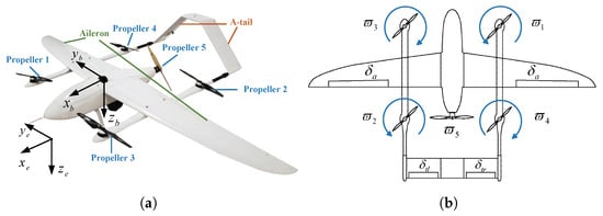
Figure 1.
Dual-syatem hybrid UAV. (a)Configuration and coordinate frames (b) Vehicle actuators.
- 1.
- Rotary-wing (RW) mode: The horizontal propulsion rotor is switched off and the position and attitude movement is controlled by differential control of the four vertical rotors, like a quadrotor.
- 2.
- Fixed-wing (FW) mode: The vertical four rotors are turned off and the vehicle behaves like an FW UAV, also known as cruise mode. Position and attitude are controlled through aerodynamic actuators and the horizontal rotor.
- 3.
- Transition mode: This mode is divided into forward transition mode and backward transition mode, which facilitate the conversion between the RW mode and the FW mode. Aerodynamic actuators and rotors are involved in the control process.
The 6-DOF dynamics of the vehicle are represented by Newton and Euler equations:
with position , velocity , Euler angles , angular rate , mass m, gravitational acceleration vector . In this paper, the left superscripts and are used to indicate in which coordinate frame the variable is defined. is the inertia matrix, expressed as
Moreover, represents transformation from body frame to earth frame and matrix is used to describe the transformation of and . , , and are forces and moments caused by propulsion system, aerodynamic effects, and disturbances.
2.2. Propulsion Forces and Moments
According to [44], the force and moment generated by each propeller are proportional to the square of the rotor speed :
where and are the thrust and moment coefficients of propeller i. Considering the same type of motor and propeller used for propellers 1-4, and . Neglecting transients in the motor, propeller speed and throttle command of each propeller are linearly related:
where and are linear model parameters.
The vehicle in Figure 1 has two separate propulsion systems, vertical and horizontal. We let and represent the forces generated by the horizontal and vertical propulsion systems. Then the total thrust can be expressed as
where denotes the force generated by propeller i.
The moment is mainly generated by the differential propeller action of the vertical propulsion system.
where d is the distance from the center of propeller (1-4) to the origin of the body frame.
2.3. Aerodynamic Forces and Moments
Different from the conventional flat and vertical tail configuration, this vehicle has an A-tail configuration. To facilitate aerodynamic and moment analysis, we convert the right and left ruddervators deflections (, ) to the elevator deflection and rudder deflection [45].
According to [46], and are defined by
with wing area S, air density , airspeed , wing span b, and mean aerodynamic chord . denotes transformation from the wind frame to the body frame. Moreover, , , , , , and are dimensionless aerodynamic coefficients, defined by [13,47]
where , , , , and denote aileron deflection angle, elevator deflection angle, rudder rotation angle, angle of attack, and sideslip angle. , , , , , , , , , , , , , , , , , , , , , . and are aerodynamic coefficients [45]. The aerodynamic moment generated by control surfaces is
where , , , , and denote the aerodynamic moment coefficients of the control surfaces.
3. Main Results
A fixed-time robust controller and control allocator constitute a unified robust nonlinear control system for dual-system hybrid UAVs. Specifically, the control scheme consists of a FxTDO and a FxTISMC. Then, control efforts generated by the attitude controller as well as the outer-loop controller are allocated to the dual-system hybrid UAV’s redundant actuators as described in Section 3.4. The attitude control framework is given in Figure 2.
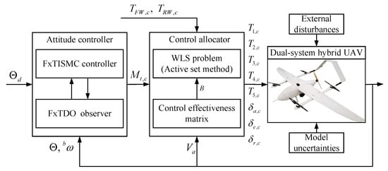
Figure 2.
Block diagram.
3.1. FxTISM Function
According to (1), the attitude dynamics are given by
By differentiating the first of (10), one has
where denotes the lumped disturbance. denotes the converted control inputs.
We let be the desired attitude angle, and then the attitude tracking error can be obtained as . We define , , and . According to (11), one can obtain
Then, a fixed-time integral sliding mode function is defined as
where
with and chosen to statisfy polynomials , hurwitz [48,49]. , , and are given by
with .
Theorem 1.
Proof.
When , one can obtain and , which yields
We denote . Then, we have
The following proof is conducted in three steps.
Step 1: prove that vector (18) is homogeneous in the bi-limit.
We define vectors and as
According to definition of homogeneity [20], vector is -homogeneous of defree with
Furthermore, vector is -homogeneous of defree with
It can be easily verified according to [20] that and are approximate vector fields of in the 0-limit and the ∞-limit. Hence, is homogeneous in the bi-limit with and .
Step 2: Prove that , and are globally asymptotically stable.
For system , we consider the Lyapunov function
where and are the ith components of and .
By differentiating (23), we have
From (25), it follows that . And when , we have . According to the LaSalle invariance principle [50], it follows that , and system is globally asymptotically stable.
For system , , consider the Lyapunov function
By differentiating (26), we have
For system , we consider the Lyapunov function
By differentiating (28), we have
From (27) and (29), we have and . According to the LaSalle invariance principle [50], it follows that , and are globally asymptotically stable.
Step 3: Prove that is fixed-time stable.
Since systems , and are globally asymptotically stable and , according to Lemma 10 [20], is fixed-time stable. Furthermore, there exist and satisfying and and a positive funcation such that function is homogeneous in the bi-limit with and , and convergence time is given as
where , , , , . □
3.2. FxTDO
For System (31), we define an auxiliary system as
where is the state of the auxiliary system. We let ; then, the error system can be obtained as a linear system as follows [26]:
where is a positive constant. , and are the state, output, and input of the system. We let , ; then, (34) can be rewritten as
We let and be estimations of and . The FxTDO for system (35) is designed as
with
where , , and are estimation errors, which can be obtained from and . Since , and , and can be calculated by and . Constants and are chosen to statisfy the polynomials , hurwitz [48,49].
Exponents , , and are selected as
where .
Theorem 2.
Proof.
The structure of the system represented by (42) and (37) is consistent with that described in (17), and the parameter design requirements are also consistent. Through the proof of Theorem 1 for the fixed-time stability of System (17), it can be seen that observation error System (42) is also fixed-time stable. Thus, the fixed-time stability proof process of the observation error system (42) is omitted here for brevity, with its convergence time denoted as .
Since for , according to (44), a fixed time convergence of is obtained. □
Remark 1.
Compared with the FxTDO [29,51,52], the designed FxTDO observer ensures that the estimation error converges to the origin rather than a bounded neighborhood. In addition, the designed observer relaxes the assumptions on disturbance, e.g., the disturbance and its derivative are assumed to be bounded [51,52,53], and upper bounds on the perturbations or their derivatives are assumed to be known [18,19,20,22].
3.3. FxTDO-FxTISMC Control Law
Theorem 3.
Proof.
We consider the Lyapunov function
According to Theorem 2, one can determine that . Thus, when , (49) can be simplified as
where , , and .
According to Lemma 2 in [30], converges to origin within fixed-time , which satisfies
When is reached, according to Theorem 1, the origin of System (17) is fixed-time stable, and the convergence time is . Finally, we can determine that attitude tracking error converges to origin within fixed time . This completes the proof. □
Remark 2.
In conventional SMC, a large switching gain is required to resist the total disturbances, resulting in chattering [22]. To eliminate chattering, a FxTDO (36) is developed to estimate the total disturbances and compensate it into SMC laws. In addition, due to the use of fractional power terms in the sliding mode surface, negative fractional power terms present in the control law which leads to the singularity problem [54]. In this work, the integral sliding mode surface (13) is used, where the fractional powers are hidden in the integral terms and no negative fractional power terms appear in the control law; thus, the proposed controller overcomes the singularity problem.
3.4. Control Allocation
We let be the total moment generated by the actuators (propellers and control surfaces). We obtain
Then, based on (4), (5), (9), and (52), one can obtain
where is the control effectiveness matrix, which can be expressed as
According to (11) and (45), the total moment commands can be obtained. and represent the thrust commands given by the outer loop controller. We let be the desired control effort and be the input commands of actuators.
The task of the control allocator is to compute the input commands of the actuators that can generate the desired control effort . Since is five-dimensional and is eight-dimensional, the vehicle is overactuated. In addition, the position and rate of the actuators are limited, i.e.,
where and are the upper and lower bounds of the ith actuator, and are the position and rate constraints of the ith actuator, and is the controller sampling time.
To effectively allocate control effort to constrained redundant actuators, this work defines the optimization allocation problem based on weighted least squares (WLS) as follows:
where and denote the diagonal weighting matrices of control and inputs, is the desired input commands, is the weighting factor, and and are the upper and lower bounds of actuators, with the elements satisfying (55), (56), and (57).
To solve this optimization Problem (58), the active set method [56] is introduced, which can efficiently handle quadratic programming problems under inequality constraints; its computational complexity is satisfied for applications in microprocessors [57].
The parameters of cost function J (58) affect the optimization results. In the folowing, we discuss parameter selection.
(1) The weighting factor is used to distinguish between primary and secondary objectives. The primary objective is to minimize in this study, so is chosen to be the larger value 1e6.
(2) For the weighting matrix , since the operating ranges of the propeller and the control surfaces are different, is chosen to normalize the range of the actuators so that the total control effort can be allocated efficiently across the different actuators.
(3) The weighting matrix is used to set the priority of the control, and we consider its equal importance, so is set as .
Remark 4.
From (54), it can be observed that thrust corresponds one to one with th thrust of Propeller 5, meaning that there are no other actuators generating thrust . Therefore, the control allocation process can be simplified by allocating to Propeller 5, while thrust and moment are allocated to the other actuators based on the WLS method.
4. Simulation Results and Discussions
In this section, to verify the control performance of the proposed fixed-time attitude controller and optimized control allocator, numerous simulations and hardware-in-the-loop (HITL) experiments are carried out on a dual-system hybrid UAV. Furthermore, the nonlinear dynamic inverse (NDI) [58] and nonsingular terminal SMC based on FTDO (FTDO-NTSMC) [16] algorithmas are used for comparison. The model parameters mentioned in Section 2 are presented in [59]. Table 1 lists the parameters of the attitude controller based on the FxTDO-FxTISMC algorithm.

Table 1.
Controller parameters of the FxTDO-FxTISMC scheme.
4.1. Attitude Tracking Simulation for RW and FW Modes
In this scenario, the reference signals are set as
And the initial attitude angles are . Note that in the FW mode, the desired yaw angle is obtained from coordinated turns.
(1) Simulation Results Without Disturbance
External disturbances and model uncertainties are not considered. Attitude tracking results for the NDI controller, the FTDO-NTSMC controller, and the FxTDO-FxTISMC controller in RW and FW modes are given in Figure 3, which shows that without disturbance, three controllers can quickly track step signals with only slight overshoot in RW mode. However, in the FW mode, the NDI controller has a larger tracking error in the orientation, while the FTDO-NTSMC controller has a longer settling time in the and orientations.
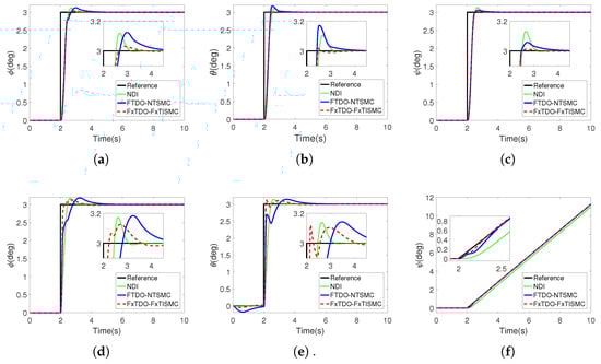
Figure 3.
Attitude tracking results for simulation without disturbance. (a) Reference and actual roll angle in RW mode. (b) Reference and actual pitch angle in RW mode. (c) Reference and actual yaw angle in RW mode. (d) Reference and actual roll angle in FW mode. (e) Reference and actual pitch angle in FW mode. (f) Reference and actual yaw angle in FW mode.
To evaluate the fast convergence ability and control accuracy of the three controllers, settling time and overshoot are introduced as performance indexes. In addition, for the comparison of yaw angle tracking control in the FW mode, the root-mean-square errors (RMSE) and integral-squared errors (ISE) are adopted as performance indexes. The quantitative results of attitude tracking in RW and FW modes are provided in Table 2 and Table 3. Table 2 shows that the proposed FxTDO-FxTISMC controller in the RW mode has the smallest overshoot performance indexes in all three directions and the smallest settling time performance indexes in the and orientations. For orientation, the proposed FxTDO-FxTISMC controller has a slightly higher settling time performance index than FTDO-NTSMC controller but lower than the NDI controller. Table 3 shows that the proposed FxTDO-FxTISMC controller has the smallest overshoot and settling time performance indexes in all orientations in the FW mode.
Table 2.
Performance comparison of step tracking without disturbance in the RW mode.
Table 3.
Performance comparison of step tracking without disturbance in the FW mode.
(2) Simulation Results With Disturbance
To verify the robustness of the proposed FxTDO-FxTISMC controller, time-varying external disturbances and aerodynamic parameter uncertaintiesis are introduced as and . In addition, turbulence disturbance (generated by the Dryden Wind Turbulence Model in simulink) and gust disturbance (generated by the Discrete Wind Gust Model in simulink) are also considered. The gust start time is 4 s, the gust length is [80 80 80] m, and the gust amplitude is [5 5 5] m/s.
Figure 4 presents the tracking results of controllers NDI, FTDO-NTSMC, and FxTDO-FxTISMC under disturbance conditions. The control performance of controllers NDI and FTDO-NTSMC deteriorates significantly after adding model parameter uncertainties and external disturbances, with significant overshoots and oscillations in both RW and FW modes. In contrast, the proposed FxTDO-FxTISMC controller exhibits strong disturbance rejection capabilities.
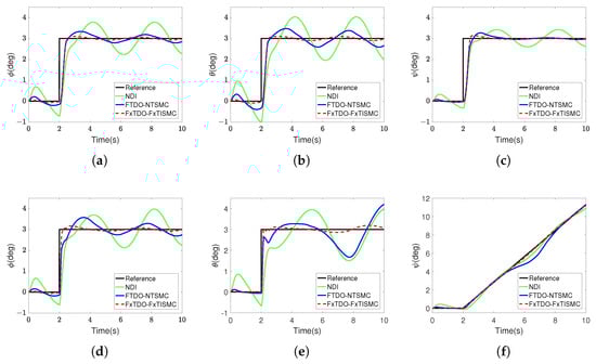
Figure 4.
Attitude tracking results for simulation with disturbance. (a) Reference and actual roll angle in RW mode. (b) Reference and actual pitch angle in RW mode. (c) Reference and actual yaw angle in RW mode. (d) Reference and actual roll angle in FW mode. (e) Reference and actual pitch angle in FW mode. (f) Reference and actual yaw angle in FW mode.
To quantitatively compare the tracking errors of the three controllers, performance indexes RMSE and ISE are calculated and summarized in Table 4 and Table 5. The proposed FxTDO-FxTISMC controller demonstrates the smallest RMSE and ISE performance indexes. Comparative results from the two simulations indicate that in comparison to the NDI and FTDO-NTSMC controllers, the proposed FxTDO-FxTISMC controller has stronger disturbance rejection capability, higher tracking accuracy, and is more suitable for attitude control of dual-system hybrid UAVs.
Table 4.
Performance comparison of step tracking with disturbance in the RW mode.
Table 5.
Performance comparison of step tracking with disturbances in the FW mode.
4.2. Simulation Results in Full Mode
In this subsection, full-mode simulation is conducted to verify the attitude control performance of the FxTDO-FxTISMC controller in full mode and the effectiveness of the proposed control allocator under conditions of constrained redundant actuators. The flight process of the hybrid UAV includes vertical takeoff in the RW mode, forward transition, cruising in the FW mode, backward transition, and vertical landing in the RW mode. The cruising airspeed of the vehicle is 21 m/s, and we consider the transition completed in the forward transition when the airspeed reaches 18 m/s and in the backward transition when the airspeed is less than 8 m/s. The desired altitude is set to 150 m except for the RW mode. The desired attitude angles are typically obtained by an outer-loop trajectory tracking controller or a path-following controller in the RW and FW modes. In this simulation, the desired roll angle in FW mode is set to to verify the tracking response of time-varying signals. In the transition mode, besides the desired pitch angle generated by the PID controller of the airspeed during the back transition, the desired attitude angles are set to zero degs. Furthermore, to prevent a significant increase in altitude caused by a large pitch angle during the backward transition, the desired pitch angle is limited to 2 degrees.
The simulation results in full mode are shown in Figure 5, and the performance indexes of attitude tracking are given in Table 6. Figure 5a–c illustrate flight trajectory, altitude, and airspeed during flight, with the forward transition completed within 3.456 s and the backward transition within 35.044 s, with a flight altitude variation within 1 m during the transition. Figure 5d–f present the results of attitude angle tracking during the flight, which show that NDI controller has a large error in tracking the time-varying signal. Table 6 shows that the proposed FxTDO-FxTISMC controller has the smallest RMS and ISE performance indexes in full-mode simulation, followed by the FTDO-NTSMC controller, with the NDI controller one being the largest. Figure 5g–i show the input commands of control surfaces and propellers, indicating that the proposed optimized control allocator can effectively allocate control forces and torques under the redundant constrained actuators.
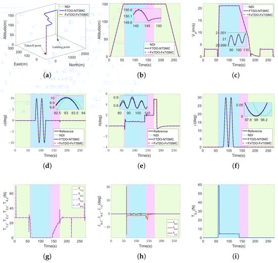
Figure 5.
State variables and control commands for the UAV in full mode (green area: RW mode, black area: FW mode, and purple area: transition mode). (a) Three-dimensional flight trajectory. (b) Altitude. (c) Airspeed. (d) Reference and actual roll angle. (e) Reference and actual pitch angle. (f) Reference and actual yaw angle. (g) Propeller 1-4 thrust command. (h) Control surface commands. (i) Propeller 5 thrust command.
Table 6.
Performance comparison in full-mode simulation.
4.3. HITL Experiment Results
To verify the engineering feasibility of the proposed attitude controller and optimized control allocator, an HITL experimental platform is established using open-source autopilot hardware. The experimental setup and workflow for the HITL experiment are given in Figure 6. The proposed attitude controller and control allocator validated in MATLAB/Simulink are compiled to generate C++ code using the Pixhawk Support Package toolbox, which is then deployed into low-cost open-source autopilot hardware. The adopted open-source autopilot used includes software and hardware systems: CUAV V5+ Autopilot (similar to a computer host) [60] and PX4 software v13.2 system (similar to an operating system and application software) [61]. The PX4 software system consists of a number of modules, each of which operates independently. After the code generated by Simulink is deployed to PX4, a new independent module (independent thread) is added to the PX4 software system to run in parallel with other modules. CopterSim software v2.54, as the core software, is used to simulate the models of UAV and sensors, as well as for communication relay [62]. UE5 software v5.2 is utilized for visualizing the vehicle and flight scenarios [63], QGroundcontrol v4.2 software is for monitoring flight status [64], and a remote controller is used for manual control. Controller parameters and flight trajectories in the HITL experiment are consistent with those in Section 4.2.
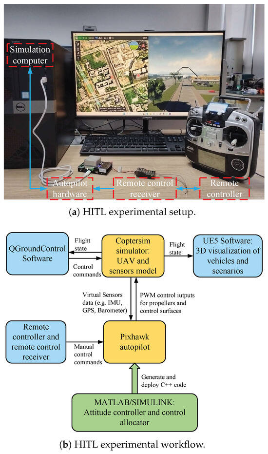
Figure 6.
HITL experimental setup and workflow.
The attitude tracking results are presented in Figure 7, with the corresponding performance indexes provided in Table 7. Due to the presence of sensor noise, there are estimation errors in the flight state, which leads to a degradation in the control performance of the three attitude controllers. In particular, the FTDO-NTSMC controller and the NDI controller exhibit significant tracking errors in pitch angle orientation, which is also confirmed by Table 7. Figure 7 and Table 7 demonstrate that compared with the FTDO-NTSMC controller and the NDI controller, the proposed FxTDO-FxTISMC controller can achieve higher tracking precision in HITL experiments.
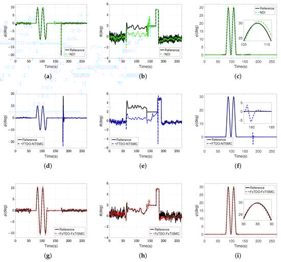
Figure 7.
Attitude tracking results in full-mode HITL experiments. (a) Reference and actual roll angle. (b) Reference and actual pitch angle. (c) Reference and actual yaw angle. (d) Reference and actual roll angle. (e) Reference and actual pitch angle. (f) Reference and actual yaw angle. (g) Reference and actual roll angle. (h) Reference and actual pitch angle. (i) Reference and actual yaw angle.
Table 7.
Performance comparison of full-mode HITL experiments.
5. Conclusions
In this study, a disturbance observer-based fixed-time control scheme for full envelope attitude control was developed for a dual-system hybrid UAV. Utilizing the fixed-time stability theory, an FxTDO was constructed to compensate for the total disturbance. Based on the designed observer, the FxTDO-FxTISMC control scheme was proposed which is robust, chatter-free, and nonsingular. Furthermore, an optimized control allocator based on the weighted least squares method was designed to map controller outputs to actuator commands. The simulation results under different flight modes and different disturbance conditions verified that the proposed controller can realize full flight mode attitude control and improve the disturbance rejection performance of the system. The HITL experiments showed that that the control algorithm has low computational complexity and can meet the requirements of a low-cost autopilot. Compared with the NDI controller and the FTDO-NTSMC controller, the proposed FxTDO-FxTISMC controller exhibited stronger robustness and higher precision.
This paper has some limitations for the design of a unified controller for a dual-system hybrid UAV: (1) Compared with the traditional SMC and linear controller, the algorithm designed in this study requires more parameters, and the current parameters need to be adjusted manually. (2) The robust attitude control, which is the main focus of this paper, is not involved in the trajectory tracking controller, especially the trajectory tracking control of the transition mode. (3) Outdoor flight experiments are not carried out due to the limitation of the experimental site and personnel. In the future, we will focus on the following issues: (1) Controller parameter adaptive adjustment: because the controller involves more parameters, when the object changes, parameter adjustment is necessary, so the design of controller parameter adaptive adjustment technology is more conducive to the promotion of the controller. (2) Unified trajectory tracking controller design: the current outer loop trajectory tracking controller is still designed according to different flight modes, and there is still a problem of controller switching. (3) Further verification of the robustness of flight control in outdoor flight environments.
Author Contributions
Conceptualization, methodology, software, and writing—original draft preparation, W.C. and L.C.; formal analysis, resources, and project administration, Z.L.; writing—review and editing, Q.D., W.Z., C.M. and T.Z.; funding acquisition, Z.L., Q.D., W.Z., C.M. and T.Z. All authors have read and agreed to the published version of the manuscript.
Funding
This research was funded in part by the Key Program of the National Natural Science Foundation of China under Grant U2433208, in part by the National Natural Science Foundation Fund under Grant 62303379, in part by the Postdoctoral Fellowship Program of CPSF under Grant GZB20240993, in part by the Natural Science Foundation of Shaanxi Province under Grant 2023-JC-QN-0665, in part by the Suzhou Municipal Science and Technology Bureau under Grant ZXL2023177 and in part by the Basic Research Program of Taicang under Grant TC2021JC09 and Grant TC2023JC13.
Data Availability Statement
The raw data supporting the conclusions of this article will be made available by the authors on request.
Conflicts of Interest
The authors declare no conflicts of interest.
References
- Ducard, G.J.; Allenspach, M. Review of designs and flight control techniques of hybrid and convertible VTOL UAVs. Aerosp. Sci. Technol. 2021, 118, 107035. [Google Scholar] [CrossRef]
- Saeed, A.S.; Younes, A.B.; Cai, C.; Cai, G. A survey of hybrid Unmanned Aerial Vehicles. Prog. Aerosp. Sci. 2018, 98, 91–105. [Google Scholar]
- Shen, S.; Xu, J.; Chen, P.; Xia, Q. Adaptive Neural Network Extended State Observer-Based Finite-Time Convergent Sliding Mode Control for a Quad Tiltrotor UAV. IEEE Trans. Aerosp. Electron. Syst. 2023, 59, 6360–6373. [Google Scholar]
- Gu, H.; Lyu, X.; Li, Z.; Shen, S.; Zhang, F. Development and experimental verification of a hybrid vertical take-off and landing (VTOL) unmanned aerial vehicle(UAV). In Proceedings of the 2017 International Conference on Unmanned Aircraft Systems, Miami, FL USA, 13–16 June 2017; pp. 160–169. [Google Scholar]
- Ansari, A.; Zhang, N.; Bernstein, D.S. Retrospective cost adaptive PID Control of quadcopter/fixed-wing mode transition in a VTOL aircraft. In Proceedings of the AIAA Guidance, Navigation, and Control Conference, Kissimmee, FL, USA, 8 January 2018. Number 210039. [Google Scholar]
- Jang, J.T.; Han, S. Analysis for VTOL Flight Software of PX4. In Proceedings of the 2018 18th International Conference on Control, Automation and Systems, PyeongChang, Republic of Korea, 17–20 October 2018; pp. 872–875. [Google Scholar]
- Silva, A.L.; Santos, D.A. Fast Nonsingular Terminal Sliding Mode Flight Control for Multirotor Aerial Vehicles. IEEE Trans. Aerosp. Electron. Syst. 2020, 56, 4288–4299. [Google Scholar]
- Wang, J.; Zhu, B.; Zheng, Z. Robust Adaptive Control for a Quadrotor UAV with Uncertain Aerodynamic Parameters. IEEE Trans. Aerosp. Electron. Syst. 2023, 59, 8313–8326. [Google Scholar]
- Manzoor, T.; Xia, Y.; Zhai, D.H.; Ma, D. Trajectory tracking control of a VTOL unmanned aerial vehicle using offset-free tracking MPC. Chin. J. Aeronaut. 2020, 33, 2024–2042. [Google Scholar]
- Allenspach, M.; Ducard, G.J. Model predictive control of a convertible tiltrotor unmanned aerial vehicle. In Proceedings of the 28th Mediterranean Conference on Control and Automation, Saint-Raphael, France, 15–18 September 2020; pp. 715–720. [Google Scholar]
- Allenspach, M.; Ducard, G.J.J. Nonlinear model predictive control and guidance for a propeller-tilting hybrid unmanned air vehicle. Automatica 2021, 132, 109790. [Google Scholar]
- Bauersfeld, L.; Spannagl, L.; Ducard, G.; Onder, C. MPC Flight Control for a Tilt-Rotor VTOL Aircraft. IEEE Trans. Aerosp. Electron. Syst. 2021, 57, 2395–2409. [Google Scholar] [CrossRef]
- Castañeda, H.; Salas-Peña, O.S.; de León-Morales, J. Extended observer based on adaptive second order sliding mode control for a fixed wing UAV. ISA Trans. 2017, 66, 226–232. [Google Scholar] [CrossRef]
- Chen, L.; Liu, Z.; Dang, Q.; Zhao, W.; Wang, G. Robust trajectory tracking control for a quadrotor using recursive sliding mode control and nonlinear extended state observer. Aerosp. Sci. Technol. 2022, 128, 107749. [Google Scholar]
- Rios, H.; Falcon, R.; Gonzalez, O.A.; Dzul, A. Continuous Sliding-Mode Control Strategies for Quadrotor Robust Tracking: Real-Time Application. IEEE Trans. Ind. Electron. 2019, 66, 1264–1272. [Google Scholar] [CrossRef]
- Wang, F.; Gao, H.; Wang, K.; Zhou, C.; Zong, Q.; Hua, C. Disturbance Observer-Based Finite-Time Control Design for a Quadrotor UAV with External Disturbance. IEEE Trans. Aerosp. Electron. Syst. 2021, 57, 834–847. [Google Scholar] [CrossRef]
- Mechali, O.; Xu, L.; Huang, Y.; Shi, M.; Xie, X. Observer-based fixed-time continuous nonsingular terminal sliding mode control of quadrotor aircraft under uncertainties and disturbances for robust trajectory tracking: Theory and experiment. Control Eng. Pract. 2021, 111, 104806. [Google Scholar] [CrossRef]
- Zhang, L.; Wei, C.; Wu, R.; Cui, N. Fixed-time extended state observer based non-singular fast terminal sliding mode control for a VTVL reusable launch vehicle. Aerosp. Sci. Technol. 2018, 82–83, 70–79. [Google Scholar] [CrossRef]
- Zhang, J.; Yu, S.; Yan, Y. Fixed-time extended state observer-based trajectory tracking and point stabilization control for marine surface vessels with uncertainties and disturbances. Ocean. Eng. 2019, 186, 106109. [Google Scholar] [CrossRef]
- Tian, B.; Zuo, Z.; Yan, X.; Wang, H. A fixed-time output feedback control scheme for double integrator systems. Automatica 2017, 80, 17–24. [Google Scholar] [CrossRef]
- Zhao, Z.L.; Guo, B.Z. A nonlinear extended state observer based on fractional power functions. Automatica 2017, 81, 286–296. [Google Scholar] [CrossRef]
- Li, B.; Zhang, H.; Xiao, B.; Wang, C.; Yang, Y. Fixed-time integral sliding mode control of a high-order nonlinear system. Nonlinear Dyn. 2022, 107, 909–920. [Google Scholar] [CrossRef]
- Cui, L.; Zhou, Q.; Huang, D.; Yang, H. Fixed-time disturbance observer-based fixed-time path following control for small fixed-wing UAVs under wind disturbances. Int. J. Adapt. Control Signal Process. 2024, 38, 23–38. [Google Scholar] [CrossRef]
- Liu, K.; Yang, P.; Wang, R.; Jiao, L.; Li, T.; Zhang, J. Observer-Based Adaptive Fuzzy Finite-Time Attitude Control for Quadrotor UAVs. IEEE Trans. Aerosp. Electron. Syst. 2023, 59, 8637–8654. [Google Scholar] [CrossRef]
- Liu, K.; Wang, R.; Zheng, S.; Dong, S.; Sun, G. Fixed-time disturbance observer-based robust fault-tolerant tracking control for uncertain quadrotor UAV subject to input delay. Nonlinear Dyn. 2022, 107, 2363–2390. [Google Scholar] [CrossRef]
- Xuan-Mung, N.; Golestani, M. Energy-Efficient Disturbance Observer-Based Attitude Tracking Control With Fixed-Time Convergence for Spacecraft. IEEE Trans. Aerosp. Electron. Syst. 2023, 59, 3659–3668. [Google Scholar]
- Huang, Y.; Jia, Y. Adaptive Fixed-Time Six-DOF Tracking Control for Noncooperative Spacecraft Fly-Around Mission. IEEE Trans. Control Syst. Technol. 2019, 27, 1796–1804. [Google Scholar]
- Zhang, J.; Yu, S.; Wu, D.; Yan, Y. Nonsingular fixed-time terminal sliding mode trajectory tracking control for marine surface vessels with anti-disturbances. Ocean Eng. 2020, 217, 108158. [Google Scholar]
- Li, B.; Gong, W.; Yang, Y.; Xiao, B.; Ran, D. Appointed Fixed Time Observer-Based Sliding Mode Control for a Quadrotor UAV under External Disturbances. IEEE Trans. Aerosp. Electron. Syst. 2022, 58, 290–303. [Google Scholar]
- Huang, Y.; Jia, Y. Robust adaptive fixed-time tracking control of 6-DOF spacecraft fly-around mission for noncooperative target. Int. J. Robust Nonlinear Control 2018, 28, 2598–2618. [Google Scholar] [CrossRef]
- Zuo, Z. Nonsingular fixed-time consensus tracking for second-order multi-agent networks. Automatica 2015, 54, 305–309. [Google Scholar] [CrossRef]
- Amrr, S.M.; Ridwan, W.; Al Dhaifallah, M.; Rezk, H. Fixed-Time Integral Sliding Mode Control with Fixed-Time Nonlinear Disturbance Observer for MPPT of Wind Turbines. Arab. J. Sci. Eng. 2025, 1–13. [Google Scholar] [CrossRef]
- Wang, X.; Wang, S. Fixed-Time Integral Terminal Sliding-Mode Control With Super-Twisting Nonlinear Extended-State Observer for Servo System With Disturbances. IEEE J. Emerg. Sel. Top. Ind. Electron. 2025, 6, 435–446. [Google Scholar]
- Sun, Y.; Van, M.; McIlvanna, S.; McLoone, S.; Ceglarek, D. Fixed-time integral sliding mode control for admittance control of a robot manipulator. Int. J. Robust Nonlinear Control 2024, 34, 3548–3564. [Google Scholar] [CrossRef]
- Jahanshahi, H.; Yao, Q.; Alotaibi, N.D. Fixed-time nonsingular adaptive attitude control of spacecraft subject to actuator faults. Chaos Solitons Fractals 2024, 179, 114395. [Google Scholar] [CrossRef]
- Zhang, D.; Hu, J.; Cheng, J.; Wu, Z.G.; Yan, H. A Novel Disturbance Observer Based Fixed-Time Sliding Mode Control for Robotic Manipulators with Global Fast Convergence. IEEE/CAA J. Autom. Sin. 2024, 11, 661–672. [Google Scholar] [CrossRef]
- Deng, Y.; Gao, H. Transition Flight Control and Test of a New Kind Tilt Prop Box-Wing VTOL UAV. In Proceedings of the 9th International Conference on Mechanical and Aerospace Engineering, Budapest, Hungary, 10–13 July 2018; pp. 90–94. [Google Scholar]
- Yuksek, B.; Inalhan, G. Transition Flight Control System Design for Fixed-Wing VTOL UAV: A Reinforcement Learning Approach. In Proceedings of the AIAA Science and Technology Forum and Exposition, San Diego, CA, USA, 3–7 January 2022; pp. 1–16. [Google Scholar]
- KAI, J.M. Full-Envelope Flight Control for Compound Vertical Takeoff and Landing Aircraft. J. Guid. Control. Dyn. 2024, 47, 1569–1585. [Google Scholar]
- Flores, G. Longitudinal modeling and control for the convertible unmanned aerial vehicle: Theory and experiments. ISA Trans. 2022, 122, 312–335. [Google Scholar] [PubMed]
- Zhang, J.; Bhardwaj, P.; Raab, S.A.; Saboo, S.; Holzapfel, F. Control allocation framework for a tilt-rotor vertical take-off and landing transition aircraft configuration. In Proceedings of the 2018 Applied Aerodynamics Conference, Atlanta, GA, USA, 25–29 June 2018; pp. 1–19. [Google Scholar]
- Pfeifle, O.; Fichter, W. Minimum Power Control Allocation for Incremental Control of Over-Actuated Transition Aircraft. J. Guid. Control Dyn. 2023, 46, 286–300. [Google Scholar]
- Johansen, T.A.; Fossen, T.I. Control allocation—A survey. Automatica 2013, 49, 1087–1103. [Google Scholar]
- Quan, Q. Dynamic Model and Parameter Measurement. In Introduction to Multicopter Design and Control; Springer: Singapore, 2017; pp. 121–143. [Google Scholar]
- Beard, R.W.; McLain, T.W. Small Unmanned Aircraft: Theory and Practice; Princeton University Press: Princeton, NJ, USA, 2012. [Google Scholar]
- Yu, Z.; Zhang, Y.; Jiang, B.; Su, C.Y.; Fu, J.; Jin, Y.; Chai, T. Nussbaum-based finite-time fractional-order backstepping fault-tolerant flight control of fixed-wing UAV against input saturation with hardware-in-the-loop validation. Mech. Syst. Signal Process. 2021, 153, 107406. [Google Scholar]
- Stevens, B.L.; Lewis, F.L.; Johnson, E.N. Aircraft Control and Simulation: Dynamics, Controls Design, and Autonomous Systems; John Wiley & Sons: Hoboken, NJ, USA, 2015. [Google Scholar]
- Basin, M.; Shtessel, Y.; Aldukali, F. Continuous finite- and fixed-time high-order regulators. J. Frankl. Inst. 2016, 353, 5001–5012. [Google Scholar]
- Kim, J.H.; Su, W.; Song, Y.J. On stability of a polynomial. J. Appl. Math. Inform. 2018, 36, 231–236. [Google Scholar]
- Khalil, H. Nonlinear Systems, 3rd ed.; Prentice Hall: Upper Saddle River, NJ, USA, 2005. [Google Scholar]
- Ma, D.; Xia, Y.; Member, S.; Shen, G.; Jiang, H.; Hao, C. Practical Fixed-Time Disturbance Rejection Control for Quadrotor Attitude Tracking. IEEE Trans. Ind. Electron. 2021, 68, 7274–7283. [Google Scholar]
- Ye, D.; Zou, A.M.; Sun, S.; Xiao, Y. A Predefined-Time Extended-State Observer-Based Approach for Velocity-Free Attitude Control of Spacecraft. IEEE Trans. Aerosp. Electron. Syst. 2023, 59, 8051–8061. [Google Scholar] [CrossRef]
- Wei, X.; Zhang, Y.; Zhang, H. Disturbance observer based fixed-time control of stochastic systems. ISA Trans. 2024, 148, 367–373. [Google Scholar] [CrossRef] [PubMed]
- Li, P.; Yu, X.; Zhang, Y.; Peng, X. Adaptive multivariable integral TSMC of a hypersonic gliding vehicle with actuator faults and model uncertainties. IEEE/ASME Trans. Mechatronics 2017, 22, 2723–2735. [Google Scholar] [CrossRef]
- Han, J. From PID to Active Disturbance Rejection Control. IEEE Trans. Ind. Electron. 2009, 56, 900–906. [Google Scholar] [CrossRef]
- Härkegård, O. Efficient active set algorithms for solving constrained least squares problems in aircraft control allocation. In Proceedings of the the IEEE Conference on Decision and Control, Las Vegas, NA, USA, 10–13 December 2002; Volume 2, pp. 1295–1300. [Google Scholar]
- Smeur, E.J.J.; Höppener, D.C.; De Wagter, C. Prioritized Control Allocation for Quadrotors Subject to Saturation. In Proceedings of the International Micro Air Vehicle Conference and Flight Competition, Toulouse, France, 18–21 September 2017; pp. 37–43. [Google Scholar]
- Harris, J.J.; Stanford, J.R. F-35 flight control law design, development and verification. In Proceedings of the Aviation Technology, Integration, and Operations Conference, Atlanta, GA, USA, 25–29 June 2018; pp. 1–18. [Google Scholar]
- Chen, L.; Liu, Z.; Dang, Q.; Zhao, W.; Chen, W. Robust fixed-time flight controller for a dual-system convertible UAV in the cruise mode. Def. Technol. 2024, 39, 53–66. [Google Scholar] [CrossRef]
- Pixhawk. Available online: https://docs.px4.io/main/zh/flight_controller/cuav_v5_plus.html (accessed on 31 December 2024).
- PX4-Autopilot. Available online: https://github.com/PX4/PX4-Autopilot (accessed on 31 December 2024).
- CopterSim. Available online: https://github.com/RflySim/CopterSim (accessed on 31 December 2024).
- Unreal Engine. Available online: https://www.unrealengine.com/en-US/ (accessed on 31 December 2024).
- QGroundControl. Available online: http://qgroundcontrol.com/ (accessed on 31 December 2024).
Disclaimer/Publisher’s Note: The statements, opinions and data contained in all publications are solely those of the individual author(s) and contributor(s) and not of MDPI and/or the editor(s). MDPI and/or the editor(s) disclaim responsibility for any injury to people or property resulting from any ideas, methods, instructions or products referred to in the content. |
© 2025 by the authors. Licensee MDPI, Basel, Switzerland. This article is an open access article distributed under the terms and conditions of the Creative Commons Attribution (CC BY) license (https://creativecommons.org/licenses/by/4.0/).