Article

Computational Fluid Dynamics (CFD)-Enhanced Dynamic Derivative Engineering Calculation Method of Tandem-Wing Unmanned Aerial Vehicles (UAVs)

1
School of Mechatronical Engineering, Beijing Institute of Technology, No. 5 Yard, Zhong Guan Cun South Street Haidian District, Beijing 100081, China
2
Yangtze Delta Region Academy of Beijing Institute of Technology, No. 1940 Yard, East North Road, Youchegang Town, Xiuzhou District, Jiaxing 314019, China
*
Author to whom correspondence should be addressed.
Drones 2025, 9(4), 231; https://doi.org/10.3390/drones9040231
Submission received: 14 January 2025 / Revised: 16 March 2025 / Accepted: 17 March 2025 / Published: 21 March 2025

Abstract

Dynamic derivatives are critical for evaluating an aircraft’s aerodynamic characteristics, dynamic modeling, and control system design during the design phase. However, due to the multiple iterations of the design phase, a method for calculating dynamic derivatives that balances computational efficiency and accuracy is required. This work presents a CFD-enhanced engineering calculation method (CEHM) for calculating tandem-wing UAVs’ dynamic derivatives. A coupling-effect-driven estimation strategy is proposed to incorporate the contribution of the rear wing to the longitudinal dynamic derivatives, and it accounts for the aerodynamic coupling effects between the front and rear wings. To enhance the accuracy of the dynamic derivative calculations, we put forward a dynamic derivative-correction mechanism based on the CFD method. It achieves three types of parameters from the static derivative CFD simulations to enhance accuracy, including parameters for aerodynamic force coefficient fitting, the dynamic pressure ratio, and the upwash and downwash gradients. The CEHM method is applied to compute the dynamic derivatives of the SULA90 tandem-wing UAV, with results compared to those obtained from the traditional engineering estimation tools (XFLR5 and OpenVSP). The simulation experiment results show that the proposed method not only calculates the acceleration derivatives but also provides higher calculation accuracy. To further validate the method’s effectiveness, open-loop model verifications were conducted using field flight test data of the SULA90. The field flight test results show that the CEHM method’s predicted results align closely with the measured flight data. The proposed method calculates dynamic derivatives in seconds, balancing accuracy and computational cost, making it highly suitable for tandem-wing aircraft during the design phase. Furthermore, this approach is generalizable and can be applied to other aircraft configurations.

1. Introduction

In recent years, tandem-wing configurations have re-emerged as a critical design option for UAVs and eVTOL vehicles due to their potential for high lift-to-drag ratios and a compact footprint [1,2,3,4,5,6]. Aligned with Munk’s stagger theorem [7], the tandem-wing configuration can potentially improve aircraft performance under optimized vertical stagger and lift distribution, leading to reduced induced drag and enhanced lift compared to conventional single-wing designs. Otherwise, this configuration combines the benefits of a morphing wing structure and wings with a relatively high aspect ratio and is widely used in the tube-launched loitering munition [8]. However, due to the more pronounced coupling effects between wings with a tandem-wing configuration compared to a traditional configuration [9], the downwash and upwash make the dynamic modeling of the tandem-wing aircraft more intricate. When modeling aircraft dynamics, three types of aerodynamic derivatives are crucial: static, control, and dynamic. Remarkably, dynamic derivatives determine an aircraft’s flying qualities. Predicting them reliably, quickly, and sufficiently early in the design stage is increasingly essential.
The aerodynamic investigation of tandem-wing aircraft primarily encompasses two key aspects. First, aerodynamic configuration optimization is investigated through parametric studies to achieve maximum aerodynamic efficiency. Researchers have conducted CFD simulations and wind tunnel experiments to analyze the effects of stagger distance, wingspan difference, and dihedral angles on flow field characteristics [1,10]. Broering et al. [11] identified the optimal chordwise spacing for lift enhancement in low-Reynolds-number regimes. Subsequent parametric studies have systematically revealed the aerodynamic coupling mechanisms of geometric parameters under such conditions [12,13,14,15]. The second aspect involves a dynamic stability investigation with the explicit consideration of coupling effects. Marcin et al. [16] discovered nonlinear relationships between span factors and dynamic stability characteristics. Tomasz et al. [17] identified directional instability and spiral–roll mode coupling in a tailless tandem-wing configuration, with a Dutch roll divergence persisting across speed ranges. The determination of dynamic derivatives predominantly employs four methodologies: wind tunnel experimentation [18], aircraft system identification [19,20,21], empirical engineering estimation [22], and computational fluid dynamics (CFD) simulations [23]. Among these, empirical estimation and CFD approaches prevail in aircraft design workflows due to their adaptability during early-stage development. The empirical estimation framework, rooted in inviscid flow theory and semi-empirical correlations, achieves high computational efficiency, including slender-body theory (SBT) [24,25], lifting-line theory (LLT) [26], lifting-surface theory (LST) [27], and the vortex lattice method (VLM) [28]. Verified for low-to-moderate angle of attack (AOA) conditions, empirical engineering estimation methods have been proven effective for calculating dynamic derivatives [29,30]. Commonly used tools include XFLR5 [31], Tornado VLM [32], AVL [33], OpenVSP [34], and DATCOM [35]. Within CFD-based approaches, dynamic derivative computation are bifurcated into time-domain and frequency-domain strategies. The time-domain methods include harmonic perturbation methods [36,37], conical motion methods [38,39,40], quasi-steady methods [41,42,43], and forced oscillation methods [44,45,46]. Frequency-domain methods primarily rely on the harmonic balance method (HBM) and its variants [47,48,49,50,51].
While contemporary CFD techniques have become the predominant approach for dynamic derivative analysis due to their high fidelity, the substantial computational overhead imposes critical constraints on design iteration efficiency, which is particularly acute in the concept design phase, where rapid responsiveness is essential. There remains an urgent need for tandem-wing aircraft aerodynamic analysis to develop dynamic derivative-prediction methodologies that balance moderate accuracy with computational efficiency. Grigorios et al. [52] developed a framework for the direct calculation of stability derivatives based on the unsteady subsonic 3D Source and Doublet Panel Method (SDPM), integrating empirical engineering estimation methods. They applied this framework to a Blended Wing Body (BWB) configuration and demonstrated that the static aerodynamic derivatives closely matched those obtained from CFD methods. However, the study did not compare the dynamic aerodynamic derivative results. Gao et al. [53] developed a dynamic modeling approach for a tandem-wing aircraft, where static and control derivatives were obtained via CFD simulations, and dynamic derivatives were calculated using the Tornado Vortex Lattice Method (VLM) tool. However, the calculation of dynamic derivatives did not utilize the results from static derivative CFD simulations, and the results lacked proper validation. The study conducted by Wang et al. [54] involved a tandem-wing aircraft weighing 4.3 kg and utilized lift curve slopes obtained from static derivative CFD simulations in conjunction with computational engineering methods to determine the longitudinal dynamic derivatives. However, it did not extend to the computation of acceleration and lateral-directional dynamic derivatives, and the interaction effects between the front and rear wings were not taken into account. Lua et al. [55] investigated the influence of installation angles and the distance between the two wings, deriving an approximate mathematical model to describe the relationship between these parameters. Zhang and Yu [9] investigated the coupling effects between the front and rear wings during the unsteady deployment process of a foldable tandem-wing UAV under low-Reynolds-number conditions. Their study revealed that the horizontal and vertical distances between the wings, as well as the wing deflection angle, significantly impact the coupling effects. However, these studies primarily focused on the factors influencing the coupling effect without examining its impact on dynamic derivatives or deriving formulas for such derivatives.
Since static derivative CFD simulations do not involve extensive unsteady calculations, their computational time is significantly less than that of dynamic derivative CFD simulations. Therefore, combining static derivative CFD simulations with empirical engineering estimation methods for dynamic derivative calculation has emerged as a viable approach. We propose a CFD-enhanced dynamic derivative engineering calculation method (CEHM) of tandem-wing UAVs. This method corrects the empirical calculation formulas for dynamic derivatives by incorporating the aerodynamic characteristics of tandem-wing aircraft. Three types of aerodynamic parameters are extracted from high-fidelity static derivative CFD simulation results to enhance the accuracy of the calculations. Three types of aerodynamic parameters are extracted from high-fidelity static derivative CFD simulation results to enhance the accuracy of the calculations. The proposed method not only calculates acceleration derivatives, which traditional empirical engineering estimation tools cannot, but also provides higher calculation accuracy. The rest of the paper is organized as follows: Section 2 introduces the aerodynamic configuration of a typical tandem-wing UAV and the model structure for aerodynamic force and moment coefficients. Section 3 demonstrates the coupling-effect-driven estimation strategy for dynamic derivative calculation. We also propose the dynamic derivative correction mechanism based on the CFD method for improving the accuracy. Section 4 presents the technical parameters of the research object. The results calculated using the CEHM method and two aerodynamic estimation tools (XFLR5 and OpenVSP ) are compared with the dynamic derivative CFD simulation results. Finally, field flight tests are conducted for open-loop model validation. Section 5 concludes the paper and provides an outlook on future work.

2. Tandem-Wing UAV Model Structure

2.1. Tandem-Wing UAV Configuration

The tandem-wing UAV discussed in this paper features a configuration with a high aspect ratio of both the front and rear wing, as shown in Figure 1a. The center of gravity (CG) of the UAV is located between the front and rear wings, which makes the contribution of the front wing to the pitching moment significant impossible to ignore. Here, b * represents the wingspan, c * represents the wing chord, and l * represents the distance from the aerodynamic center AC to the CG, measured along the body axis. The subscript (*) denotes different aerodynamic components, f w represents the front wing, r w represents the rear wing, and v t represents the vertical tail. It is assumed that the AC of each aerodynamic component is located at one-quarter of its chord length. As shown in Figure 1b, z is the rolling moment arm of the vertical tail, and z v t is the vertical distance from the AC of the vertical tail to the aircraft reference line, measured normally to the body axis. The relationships between z, z v t and l v t are
z = z v t cos α l v t sin α ,
where α denotes the angle of attack (AOA).
The reference wing area S, reference wing span b, and reference wing chord c are defined as
S = b f w c f w + b r w c r w
b = b f w
c = c f w

2.2. Aerodynamic Model Structure

For small UAVs, the effects of Froude, Mach, Strouhal, and Reynolds numbers are generally neglected, and the mass and inertia of the aircraft dominate those of the surrounding air [19,56]. A general model of the aerodynamic forces and moments acting on a fixed-wing UAV is given in Equation (5) [57].
D Y L = 1 2 ρ V a 2 C D α , α ˙ , β , p , q , r , δ a , δ e , δ r C Y α , β , β ˙ , p , q , r , δ a , δ e , δ r C L α , α ˙ , β , p , q , r , δ a , δ e , δ r L A M A N A = 1 2 ρ V a 2 b C l α , β , β ˙ , p , q , r , δ a , δ e , δ r c C m α , α ˙ , β , p , q , r , δ a , δ e , δ r b C n α , β , β ˙ , p , q , r , δ a , δ e , δ r ,
where ρ denotes air density, V a represents airspeed, and dynamic pressure is defined as Q = 1 2 ρ V a 2 . β is the angle of sideslip (AOS), while α ˙ and β ˙ signify the rates of change of AOA and AOS, respectively. Angular rates p, q, and r correspond to rotational velocities about the X b , Y b , and Z b axis of the body frame F b . δ a , δ e , and δ r are the controls of the aileron, elevator, and rudder. D, Y, and L are the aerodynamic drag, side, and lift forces, acting along the negative X w , positive Y w , and negative Z w axis of the wind frame F w . The dimensionless aerodynamic coefficients for these forces are C D , C Y , and C L , respectively. L A , M A , and N A are the aerodynamic rolling, pitching, yawing moments, acting along the X b , Y b and Z b axes. The dimensionless aerodynamic coefficients of these moments are C l , C m , and C n .
A commonly adopted simplification assumes decoupled longitudinal and lateral dynamics for UAVs operating at a small AOA and AOS. Under this paradigm, the lift force coefficient C L and pitch moment coefficient C m depend on α , α ˙ , q and δ e while remaining independent of lateral-directional variables β , p, r, δ a and δ r . Conversely, the roll C l and yaw C n coefficients, on the other hand, are independent of α , q, and δ e and are related to β , p, r, δ r and δ a . Notably, a residual coupling persists through the AOS-dependent drag force, which retains bidirectional sensitivity due to airframe symmetry about the X w Z w -plane, rendering the drag force coefficient C D an even function of β .
In summary, the aerodynamic force and moment coefficients are expressed in Equation (6), and each aerodynamic coefficient comprises three parts: static, control, and dynamic derivatives.
C D C Y C L = C D α + Δ C D β + Δ C D δ e + C D q q ¯ C Y β + Δ C Y δ r + C Y r r ¯ C L α + Δ C L δ e + C L q q ¯ + C L α ˙ α ˙ ¯ C l C m C n = C l β + Δ C l δ a + Δ C l δ r + C l p p ¯ + C l r r ¯ C m α + Δ C m δ e + C m q q ¯ + C m α ˙ α ˙ ¯ C n β + Δ C n δ a + Δ C n δ r + C n p p ¯ + C n r r ¯ ,
where q ¯ = q c 2 V a , α ˙ ¯ = α ˙ c 2 V a , p ¯ = p b 2 V a , r ¯ = r b 2 V a .
Static derivatives are aerodynamic derivatives related to the airflow angle, including α and β . A lookup table method is used for modeling, including C D α , Δ C D β , C Y β , C L α , C l β , C m α , and C n β . Taking the non-deflected state as the baseline, the effects of control surface deflections are expressed incrementally and also modeled using lookup tables, including Δ C D δ e , Δ C Y δ r , Δ C L δ e , Δ C l δ a , Δ C l δ r , Δ C m δ e , Δ C n δ a and Δ C n δ r . Dynamic derivatives mainly consist of angular rate derivatives associated with three-axis angular rates and acceleration derivatives related to airflow angular rates. The angular rate derivative is a key component of the dynamic derivatives and plays a major role in aircraft dynamics and control. Due to the use of a decoupling modeling approach, the angular rate derivatives considered in this paper include C D q , C Y r , C L q , C l p , C l r , C m q , C n p , and C n r . Although the effect of the acceleration derivatives is relatively small, this paper considers the AOA acceleration derivatives C L α ˙ and C m α ˙ for modeling the aerodynamic characteristics of the highly maneuverable flight. The AOS rate β ˙ has a minor influence than the roll angular rate p and the yaw angular rate r, so the AOS acceleration derivatives are neglected [58]. Dynamic derivatives are modeled using constant parameters. This paper assumes metric units in the aerodynamic model, with angles, including control surface deflections, and angular rates provided in radians and radians per second.

3. CFD-Enhanced Dynamic Derivative Engineering Estimation Method (CEHM)

3.1. Coupling the Effect-Driven Estimation Strategy

3.1.1. Longitudinal Dynamic Derivatives

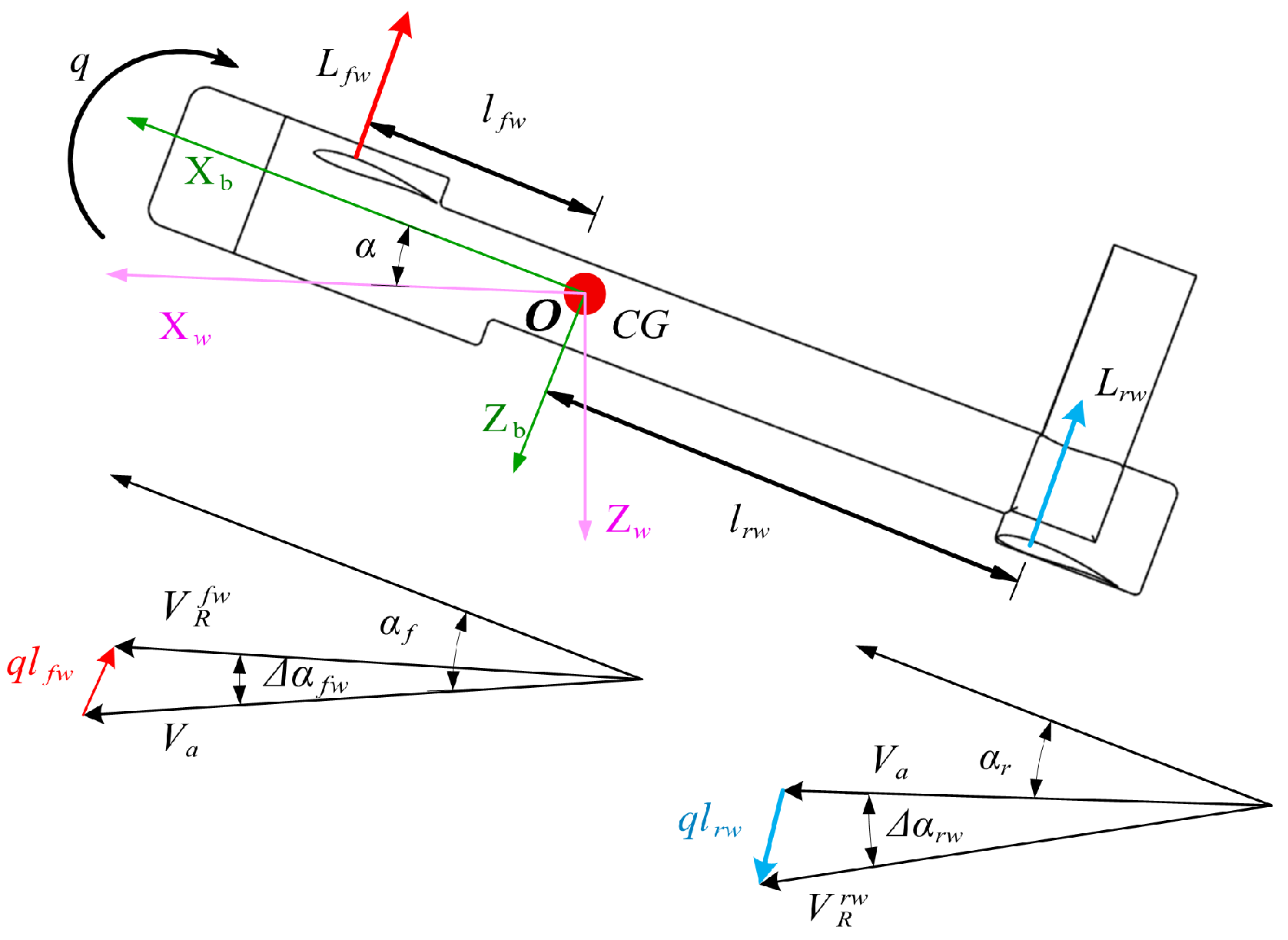
For conventional configurations, when the CG resides near the AC, the horizontal tail demonstrates a more substantial effect on longitudinal stability derivatives compared to the wing [22]. However, in tandem-wing UAV architectures, the CG is typically located between the front and rear wings, resulting in both lifting surfaces contributing dominantly to stability derivative characteristics. As shown in Figure 2, the flight AOA of UAV is α . By considering the downwash effect from the front wing on the rear wing (inducing a downwash angle of attack, ε ) and the upwash effect from the rear wing on the front wing (inducing an upwash angle of attack, ϑ ), the actual effective AOAs for the front wing and rear wing become α f = α + ε and α r = α ϑ , respectively. Static aerodynamic derivatives obtained through Reynolds-Averaged Navier–Stokes (RANS) simulations inherently capture these bidirectional interference effects. To align with the CFD framework, all aerodynamic coefficients (e.g., lift, drag, and moments) are expressed as functions of the UAV’s flight AOA α , rather than the effective angles ( α f or α r ). For example, the front wing’s lift coefficient C L f w α derived from CFD simulations represents the actual lift force when the AOA is α f = α + ε , even though it is parametrized in terms of α . Similar reasoning applies to the rear wing’s coefficients. Detailed methodologies for processing CFD results are provided in Section 3.2.
We assume that the UAV undergoes a positive pitch rate q for the front and rear wings, the AOA variation of the front wing is Δ α f w = q l f w V a , the AOA variation of the rear wing is Δ α r w = q l r w V a , and the detailed derivations are given in Appendix A.1. We define the downwash gradient of the rear wing as d ε d α and the upwash gradient of the forewing as d ϑ d α . The upwash angle variation Δ ϑ on the front wing induced by the rear wing’s AOA variation Δ α r w is quantified as Δ ϑ = d ϑ d α Δ α r w . Correspondingly, the downwash angle variation Δ ε on the rear wing induced by the front wing’s AOA variation Δ α f w is quantified as Δ ε = d ε d α Δ α f w . Therefore, the change in the lift coefficient induced by the front and rear wing for the entire UAV can be expressed as
Δ C L f w = C L f w α + Δ α f w + Δ ϑ C L f w ( α ) = C L α f w η f w S f w S q V a l f w d ϑ d α l r w
Δ C L r w = C L r w α + Δ α r w Δ ε C L r w α = C L α r w η r w S r w S q V a l r w + d ε d α l f w ,
where Δ C L * denotes the variation in the entire aircraft lift coefficient induced by the wing, C L * α represents the lift coefficient at AOA α obtained from CFD simulations, C L α * represents the lift curve slope of the wing, η * = Q * Q represents dynamic pressure ratio, S * donates the wing area, and the subscript (*) can be f w and r w . The detailed derivation processes for Equations (7) and (8) are provided in Appendix A.1.
For brevity, we denote d ϑ d α as ϑ and d ε d α as ε . Due to the minor influence of the fuselage and vertical tail on the longitudinal dynamic derivatives, the C L q is given by
C L q = 2 · C L α r w S r w η r w l r w + ε l f w C L α f w S f w η f w l f w ϑ l r w S · c
By using a similar method, C D q and C m q are given by
C D q = 2 C D f w i · S f w + C D r w i S r w S c
C m q = 2 · C L α r w S r w η r w l r w + ε l f w l r w + C L α f w S f w η f w l f w ϑ l r w l f w S · c 2
In Equation (10),
C D f w i = C D α f w l f w + ϑ l r w + 2 C D α 2 f w α l f w + ϑ l r w
C D r w i = C D α r w l r w + ε l f w + 2 C D α 2 r w α l r w + ε l f w
where C D α * and C D α 2 * are the first- and second-order coefficients of the quadratic fitting curve of C D α , and the subscript (*) can be f w and r w . The acceleration derivatives C L α ˙ and C m α ˙ are measures of the time-lag effects on the lift force and pitching moment when the aircraft experiences a change in the AOA with respect to time. The calculation formulas are given by [22]
C L α ˙ = 2 C L α r w S r w l r w + l f w S c η r w d ε d α
C m α ˙ = C L α ˙ l r w c ,
where d ε d α is the downwash gradient at the rear wing that can be estimated using the static derivatives CFD simulation results discussed in Section 3.2.

3.1.2. Lateral-Directional Dynamic Derivatives

The lateral-directional dynamic derivatives’ calculation formulas are the same as those of traditional configuration aircraft and are given by [22]
C Y r = 2 b A C Y β v t
C l p = 2 z b z z v t b C Y β v t i f w , r w C L α i + C D i ( α ) c i b i 3 6 S b 2
C l r = 2 b 2 A B · C Y β v t + * f w , r w c * b * 3 C L * ( α ) 3 S b 2
C n p = 2 A z z v t b 2 C Y β v t * f w , r w C L * ( α ) C D α * 2 C D α 2 * α c * b * 3 6 S b 2
C n r = 2 b A 2 C Y β v t * f w , r w C D * ( α ) c * b * 3 3 S b 2 ,
where C Y β v t represents the rate of change of the vertical tail side force with respect to the AOS. C D * ( α ) is the drag force coefficient of the wing, C L * ( α ) is the lift force coefficient of the wing, and the subscript (*) can be f w and r w . In the above equations, A and B are given by
A = l v t cos α + z v t sin α B = z v t cos α l v t sin α
Thus far, we have established the estimation formulae for the dynamic derivatives of the tandem-wing UAV. The UAV’s geometric parameters, such as S, b, and c, are derived from aerodynamic design specifications. However, the aerodynamic parameters in these formulas, such as C L α * , C D α * , η * and d ε d α , conventionally rely on inviscid flow theory and semi-empirical correlations, fundamentally limiting prediction accuracy in traditional methodologies. To mitigate this constraint, the present study integrates static-derivative CFD simulation data to refine dynamic derivative computation accuracy.

3.2. Dynamic Derivative Correction Mechanism Based on the CFD Method

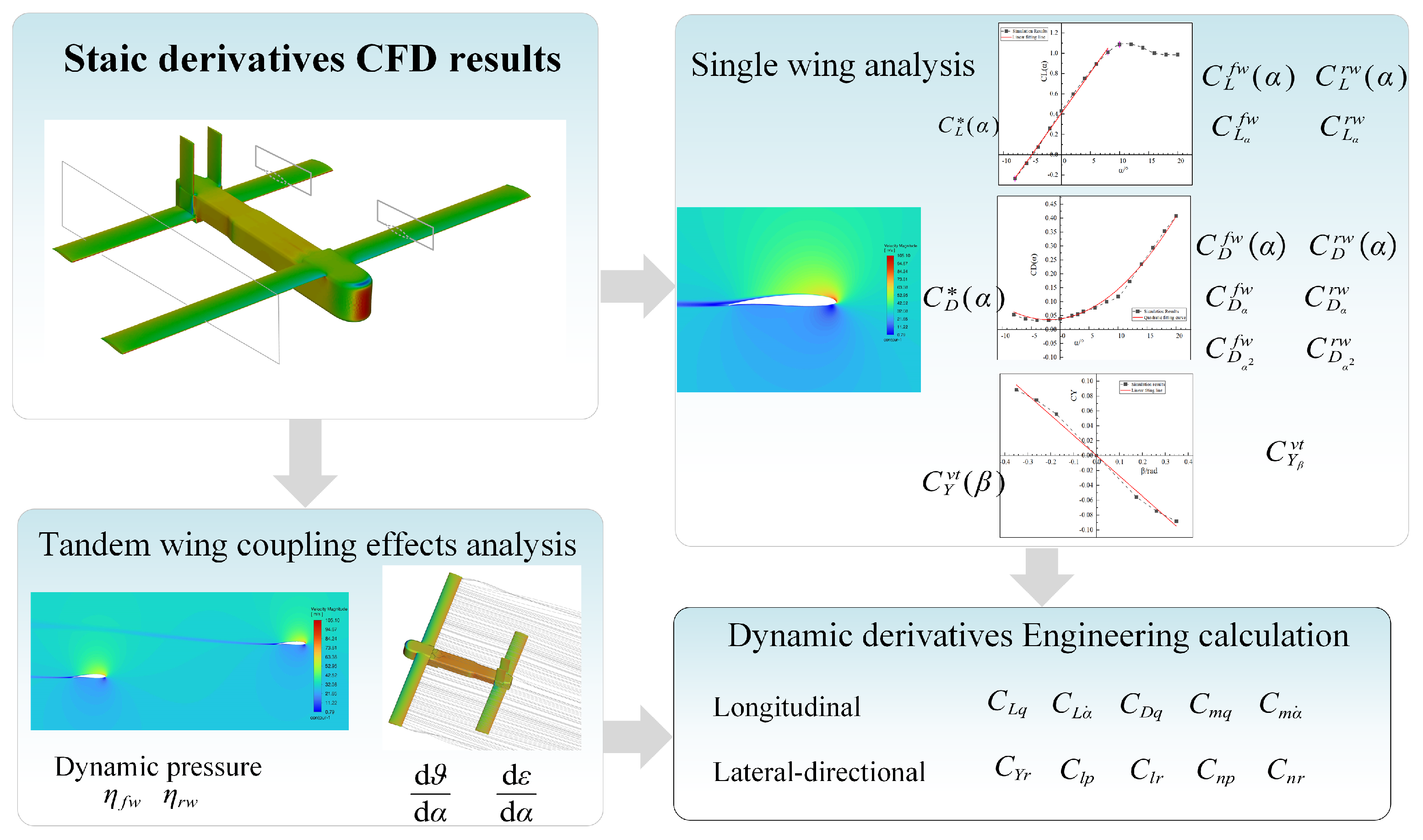
The method for enhancing the accuracy of dynamic derivatives calculations based on static derivative CFD simulation results can be broadly divided into two key aspects, as illustrated in Figure 3. The first component emphasizes the aerodynamic analysis of individual configuration elements. This involves analyzing the CFD simulation data for the front and rear wing to extract fitting parameters related to the lift and drag force coefficients as a function of the AOA, as well as for the vertical tail, to obtain the fitting parameters related to the side force coefficient as a function of the AOS. The second component investigates aerodynamic coupling between the front and rear wings. This includes measuring the dynamic pressure on both wings to compute the dynamic pressure ratio, calculating the washout gradient of the rear wing caused by the downwash effect from the front wing and the upwash gradient of the front wing caused by the rear wing.
Through this analysis, three types of aerodynamic parameters are derived.
(1)
The aerodynamic-force-related parameters. Within the linear range of the lift coefficient variation, the lift force coefficient data for both the front and rear wings, as functions of AOA, are typically modeled using a linear function, as shown in Equation (22). The drag coefficient data for both the front and rear wings, as a function of AOA, are generally approximated with a quadratic polynomial, as depicted in Equation (23). Similarly, the side force coefficient data for the vertical tail as a function of AOS are fitted with a linear function, as indicated in Equation (24).
C L * α = C L 0 * + C L α * α
C D * α = C D 0 * + C D α * α + C D α 2 * α 2
C Y v t β = C Y β v t · β ,
where the subscript (*) can be f w and r w .
(2)
The dynamic pressure ratios. The dynamic pressure measured one body length from the nose is the reference dynamic pressure Q. The dynamic pressures measured at a quarter chord length from the leading edge of the front and rear wings are referred to as the front wing dynamic pressure Q f w and the rear wing dynamic pressure Q r w , respectively. Therefore, the formulas for calculating the front and rear wing dynamic pressure ratios are as follows:
η f w = Q f w Q
η r w = Q r w Q
(3)
The rear wing washout and front upwash gradient. To investigate the aerodynamic interactions between the front and rear wings, static CFD simulations were conducted, excluding the standalone wings for comparison. The rear wing lift coefficient from the CFD simulation omitting the front wing is denoted as C L r w s i α , and the front wing lift coefficient from the simulation omitting the rear wing is C L f w s i α . In the full-aircraft static derivative CFD simulation, the rear wing lift coefficient is C L r w α and the front wing lift coefficient is C L f w α . Using the rear wing lift curve slope derived from Equation (22), the downwash gradient d ε d α on the rear wing at this AOA is calculated using Equation (27). Similarly, the upwash gradient d ϑ d α on the front wing is calculated using Equation (28).
d ε d α = d C L r w s i α C L r w α C L α r w / d α
d ϑ d α = d C L f w α C L f w s i α C L α f w / d α

4. Simulation and Field Experimental Results

4.1. SULA90 UAV

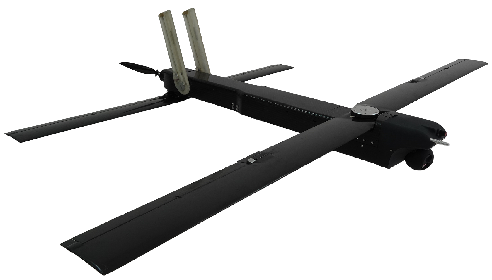
The research object in this paper is a 10 kg class UAV, named SULA90 [58,59], which is designed by the Beijing Institute of Technology, as shown in Figure 4. This small, tandem-wing UAV utilizes a conventional control setup, featuring ailerons on the front wings, elevators on the rear wings, and rudders on the vertical tails. It is powered by a single electric motor positioned at the rear of the fuselage, which drives a custom-designed, carbon-fiber folding propeller. The UAV’s geometric and inertial properties are detailed in Table 1.

4.2. Reference Values Obtained by Dynamic Derivative CFD Simulations

To verify the effectiveness of the proposed method, this paper uses the dynamic derivative CFD simulations as reference values. We calculate the dynamic derivatives in both the longitudinal and lateral directions. A forced oscillation analysis method with a simple harmonic oscillation (SHO) mode is adopted to obtain longitudinal coupled dynamic derivatives C * q + C * α ˙ [45,60], and the quasi-steady method is used for solving the longitudinal angular rate derivative C * q [43], where the subscript * is L, D and m. Researchers have applied the aforementioned method for dynamic derivative CFD simulations across different flight platforms and have validated its effectiveness using wind tunnel data [46,61]. According to Equation (6), we only need to consider the angular rate derivatives for the roll and yaw directions. Therefore, steady roll and yaw movements are simulated to obtain the C * p and C * r , where the subscript * can be Y, l, and n. As the UAV primarily operates in cruise flight, the CFD simulation uses a cruise flight speed of 30 m/s and an altitude of 300 m above sea level. All numerical simulations were conducted in ANSYS FLUENT 2023R1 with tailored methodologies for distinct aerodynamic derivatives. For the longitudinally coupled dynamic derivatives, a transient solver is employed, a transient pressure-based solver incorporating the Sliding Mesh Method (SMM) [62] was used to simulate UAV oscillatory motions, utilizing the realizable k ε turbulence model with standard wall functions. The first-order implicit transient formulation is utilized, with the Roe-FDS flux scheme and cell-based gradient reconstruction for the least squares applied for numerical accuracy. The second-order upwind scheme is used for spatial discretization. The Courant number is set to 20, and default under-relaxation factor values are employed. A fixed-time-step-size marching scheme with the user-specified method is implemented to ensure stability and precision. In parallel, the angle rate derivatives simulations implemented a steady-state framework through the Multiple Reference Frame (MRF) [63] approach, retaining an identical turbulence model while adopting a coupled pressure–velocity solver for enhanced convergence. Spatial discretization preserved second-order upwind accuracy with identical Courant number conditioning, complemented by standardized relaxation factors.
The entire computational fluid domain is a spherical region with a diameter of 20 m. Using ANSYS Fluent Meshing 2023R1, an unstructured computational grid was generated. The process began with the creation of a triangular surface mesh, followed by the configuration of boundary layer parameters, and concluded with the generation of a poly-hexcore volume mesh. In this context, the first layer’s height and the number of boundary layers are directly linked to the Y p l u s value, which is determined by the turbulence model employed in the simulation. For RANS-based CFD simulations of external aerodynamic flows, three turbulence models are typically used: Spalart–Allmaras (SA), k ε , and k ω . The SA model is a single-equation approach and performs well for simple geometries but shows limitations in predicting shear and separated flows. The k ω model is a two-equation approach; while offering high accuracy for boundary layer resolution, it imposes stringent grid requirements ( Y p l u s 1 and at least 15 boundary layers). For example, achieving Y p l u s = 1 on the SULA90 would require a first-layer thickness of 0.01 mm, significantly increasing mesh density and compromising grid quality at wing–body junctions due to extreme aspect ratios. To balance accuracy and computational efficiency, the realizable k ε model was selected. This model permits a relaxed Y p l u s threshold of 30 and a reduced boundary layer count of 10 while still capturing essential boundary layer physics. The first layer’s height was set to 0.3 mm using the last ratio offset method with a transition ratio of 0.272 . The UAV surface mesh and boundary layers on the UAV wall are depicted in Figure 5a. The far field was assigned a pressure–far-field boundary condition, while the UAV wall was defined as the no-slip wall.
The Sliding Mesh Method (SMM) is a dynamic mesh technique for or longitudinal coupled dynamic derivative simulations. The fluid domain is partitioned into static and dynamic zones, as shown in Figure 5b. The dynamic zone encompasses the mesh within a 5 m diameter inner sphere and the UAV wall, actuated by longitudinal oscillatory motions governed by a User-Defined Function (UDF) file, while the static zone extends to the far-field boundary. In contrast, angular rate derivatives simulations are steady-state simulations, only requiring a single fluid domain, though configured with corresponding rotational velocities to replicate the UAV’s uniform rotation. The longitudinal coupled dynamic derivative case utilized a volumetric mesh comprising 11.867 million elements, whereas the angular rate derivatives case employed 9.192 million elements. The above simulations were run on a workstation AMD EPYC 9554 series 128-core CPU, finishing in 64 h and 20 min. The detailed procedure is as follows.
(1) Longitudinal coupled dynamic derivative analysis: The AOA vibration equation is given by
α = α 0 + α m sin ω t ,
where α 0 is the initial flight AOA and is set as zero, and the oscillation amplitude α m is set as 2 deg. The equation of the oscillation angular rate is ω = 2 V a k c . In the equation, the reduced frequency k = 0.02 , V a = 30 m / s , so ω = 9.23077 rad / s . The numerical simulations adopt a fixed time step ( Δ t = 0.02 s) with a convergence threshold limiting iterations to 50 per step. A total of 144 time steps are calculated, thereby yielding a complete harmonic oscillation period of 2.88 s. The results from 2.1 to 2.88 s were fitted using the Least Squares Method (LSM). The C L and C m fitting formula is shown in Equation (30), and the C D fitting formula is shown in Equation (31).
C * = C * 0 + C * α α m sin ω t + C * q + C * α ˙ k α m cos ω t ( * = L , M )
C D = C D 0 + C D α Δ α + C D α ˙ α ˙ c 2 V + C D q q c 2 V + 1 2 C D α 2 Δ α 2
The fitting curves of C L , C m and C D for the whole SULA90 are shown in Figure 6a–c. The fitting curves of C L f u s , C m f u s and C D f u s for the fuselage are shown in Figure 7a–c. The detailed computational method for longitudinal coupling derivatives is presented in Appendix A.2.
(2) Longitudinal pitch angular rate derivative analysis: The AOA is also set to zero, and the pitch rate q is taken as 2.4 rad / s , 5 rad / s , 10 rad / s , and 15 rad / s . A linear fit is used to analyze how C L , C m and C D change with respect to q ¯ ( q ¯ = q c 2 V a ), as shown in Figure 8a. The slope of the fitting line represents the pitch angular rate derivative C * q , where the subscript * can be L, D and m.
Table 2 shows the detailed longitudinal dynamic derivative results for the whole UAV and the fuselage. It can be observed that the fuselage primarily affects the drag dynamic derivatives (e.g., C D q f u s and C D α ˙ f u s ) while having minimal impact on the lift dynamic derivatives (e.g., C L q f u s and C L α ˙ f u s ) and pitching moment dynamic derivatives (e.g., C m q f u s and C m α ˙ f u s ).
(3) Lateral-directional angular rate derivative analysis: The AOA is also set to zero, and the roll rate p is taken as 0.1 rad / s , 0.4 rad / s , 0.6 rad / s , and 1 rad / s for a total of four simulations. A linear fit is used to analyze how C l and C n change with respect to p ¯ ( p ¯ = p b 2 V a ), as shown in Figure 8b. The slope of the fitting line represents the roll angular rate derivatives, so we obtain C l p = 0.7513 and C n p = 0.11066 . The AOA and yaw rate r are the same as roll angular rate derivative analysis. A linear fit is used to analyze how C Y , C l and C n change with respect to r ¯ ( r ¯ = r b 2 V a ), as shown in Figure 8c. The slope of the fitting line represents the yaw angular rate derivatives, so we obtain C l r = 0.5491 and C n r = 0.1106 and C Y r = 0.6888 .

4.3. Comparison Results

Research indicates that the accuracy of dynamic derivatives depends on the chosen control method. The aircraft primarily employs two control methods: open-loop and closed-loop control. Compared to closed-loop control, open-loop control demands higher precision [22,64]. W. B. Blake [30] summarized the accuracy criteria for both methods in Table 3. Since the modern UAV primarily utilizes closed-loop control, the proposed method meets the precision requirements for closed-loop control, which means it is suitable for engineering applications. So, the relative difference of the longitudinal dynamic derivative should not exceed 50 % , and the absolute difference of the lateral-directional derivative should not exceed 0.2 /rad.
The dynamic derivative calculations in the CEHM method require three types of aerodynamic parameters, which are derived from static derivatives CFD simulation results. The CFD simulations used in the CEHM are presented in Appendix A.3, while the calculation process and results of the three types of parameters are provided in Appendix A.4 and the detailed results of the static derivatives CFD simulations are provided in Appendix A.5. To validate the effectiveness of the CEHM method, two widely used aerodynamic estimation software tools were employed for comparison: XFLR5 (version 6.61) and OpenVSP (version 3.41.2). Since the CEHM method omits the influence of the fuselage when estimating dynamic derivatives, XFLR5 and OpenVSP also neglect fuselage effects to ensure consistency in the calculations. The simulation models for these tools are shown in Figure 9. The computation times for CEHM and XFLR5 are on the order of seconds, while OpenVSP requires minutes. The CFD simulations employed as input for CEHM required 24 h and 46 min, equating to a quarter of the computational duration entailed by traditional full-CFD methods. The dynamic derivative results calculated at zero AOA are summarized in Table 4. Using the CFD simulation results as the reference values, we evaluate the effectiveness of the CEHM method by calculating the relative differences for longitudinal dynamic derivatives and the absolute difference for lateral-directional dynamic derivatives.
The relative differences (RDs) for the dynamic derivatives are summarized in Table 4. To facilitate a more meaningful comparison, the dynamic derivatives in the CFD calculation results provided in the table are adjusted by subtracting the fuselage effects according to Table 2. Given the relatively minor influence of the fuselage on lateral-directional dynamic derivatives, the CFD-derived lateral-directional dynamic derivatives presented in the table are based on full-aircraft computational results. For C L q , the relative differences for the CEHM method remain below 25 % , satisfying the stringent criteria for open-loop control. The relative differences for XFLR5 and OpenVSP closely approach 25 % . Regarding C m q , all three methods exhibit relative differences within 15 % , with the CEHM method achieving the highest precision at a relative difference of 4.61 % . While XFLR5 is incapable of computing C D q , OpenVSP demonstrates a substantial relative discrepancy of 48.1 % , which aligns with closed-loop control prerequisites. In contrast, the CEHM method yields a relative difference of 20.36 % for C D q , which meets the open-loop control requirement. Furthermore, XFLR5 and OpenVSP lack the capability to compute acceleration derivatives such as C L α ˙ and C m α ˙ , which are critical for simulating high-maneuverability flight dynamics. The CEHM method, conversely, not only calculates these acceleration derivatives but also attains an acceptable accuracy. For C Y r , both XFLR5 and OpenVSP exhibit relative errors exceeding 80 % , whereas the CEHM method demonstrates the smallest relative difference at 34.96 % , accompanied by an absolute difference of 0.2408 /rad, as illustrated in Table 4; this value approaches the permissible tolerance range. For C l r and C l p , only the CEHM method produces results within the required accuracy. For C n r and C n p , although all three methods meet the requirements, the CEHM method achieves the highest accuracy, with an absolute difference of about half of the results from XFLR5 and OpenVSP.

4.4. Open-Loop Validation of the Models Based on Field Flight

4.4.1. Validation Process and Metrics

To further validate the effectiveness of the method proposed in this paper, we employed an open-loop model verification approach based on field flight data [54], with the framework shown in Figure 10. We use the open-source Flight Dynamic Model software (FDM) code JSBSim [65,66] to develop the CEHM method FDM named the CEHM plant, which uses CFD simulation results for static and control derivatives; the detailed derivatives are in Appendix A.4. Still, its dynamic derivatives are obtained using the CEHM method. Two pitch and roll maneuver data segments from the flight test data are selected for individual validation. The control surface deflections from these data segments are used as inputs to the FDM. The inputs are fed into the CEHM plant, and the predicted angular rates are compared with the measured data. The pitch control surface output in the flight test data is denoted as δ e r e , the roll control surface output is δ a r e , the recorded pitch angular rate is q r e , and the recorded roll angular rate is p r e . In the predicted outputs from the FDM, the predicted pitch angular rate is denoted as q p r and the predicted roll angular rate as p p r . The control surface deflections for roll and yaw should be 0 or near 0 in the pitch maneuver flight data segment to minimize interference from different control inputs. Similarly, the control surface deflections for pitch and yaw should also be 0 or near 0 for the roll maneuver flight data segment.
The goodness of fit between the model’s predicted output and the measured values is evaluated using the coefficient of determination ( R 2 ) and the root mean square error ( R M S E ) [67], as shown in Equations (31) and (32), respectively. A value of R 2 closer to 1 indicates a better fit, while values closer to 0 suggest a poor fit. Similarly, an R M S E value closer to zero indicates that the model’s predicted values are closer to the measured data, reflecting a better model fit.
R 2 = 1 i = 1 n X i Y i 2 i = 1 n Y ¯ Y i 2
RMSE = 1 n i = 1 n X i Y i 2 ,
where X i is the predicted ith value and Y i is the actual ith value. Y ¯ is the mean of the actual values, and Y ¯ = 1 n i = 1 n Y i . n is the total number of the values.

4.4.2. Field Flight Data Collection

The electrical components of SULA90 are shown in Figure 11. It is equipped with an onboard Pixhawk autopilot named CUAV X7+ Pro. The autopilot is running PX4 firmware and records the flight data in ulog form. The sensor package includes a Global Positioning System (GPS) receiver and an airspeed sensor. Pulse width modulation (PWM) control signals applied to the control surface actuators are recorded and mapped using a servo-actuator model to control surface deflection angles. The sample rate for the translational acceleration and angular rate measurements is 200 Hz. The sample rate for the EKF-derived data is 100 Hz. The control effector PWM commands and the propeller rotational speed are sampled at 50 Hz.
The field flight used for this paper is only conducted in negligible wind conditions. The test adopts a taxi takeoff method, and the total test flight time is 6 min 42 s. We set a rectangular flight route to collect flight data for model validation, as shown in Figure 12, and it should be noted that the entire flight process is not shown in the figure. The pitch maneuver data segment is selected from the steady-level flight phase, where the roll and yaw deflections are small. The roll maneuver data segment is selected from the turn flight phase, with small pitch and yaw deflections.

4.4.3. The Model Validation Results

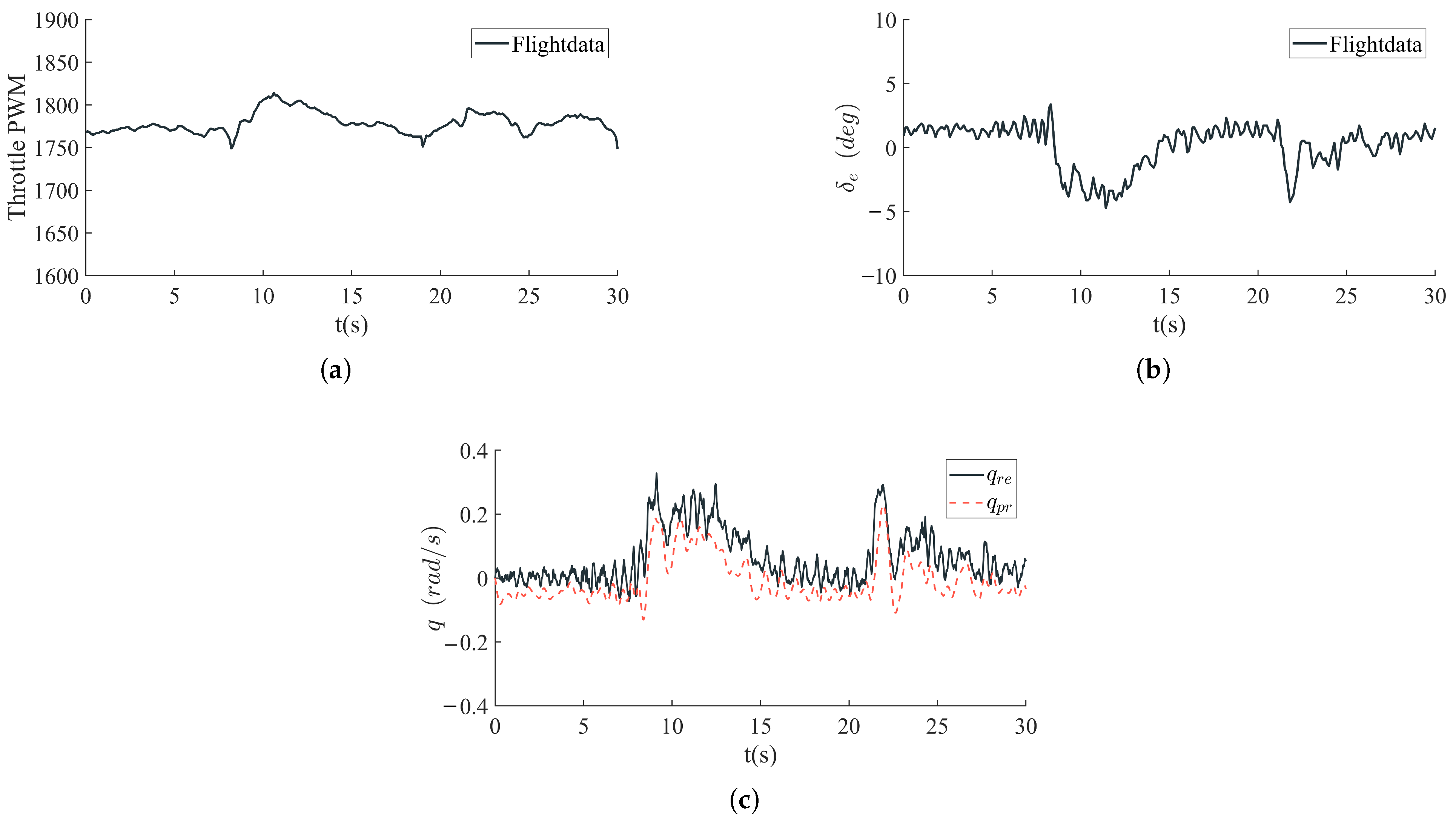
A 20 s flight data segment, from 163 s to 183 s, was extracted for roll maneuver analysis. The aileron control input δ a r e is shown in Figure 13a, and two lateral maneuvers with turns can be observed. As illustrated in Figure 13b, the results of the CEHM plant are acceptable. The RMSE between p p r and p r e is 0.102 rad / s , and the R 2 is 0.7829 . A segment data with relatively constant throttle output is used to minimize the influence of throttle input variations, as shown in Figure 14a. The input is a total of 30 s of steady straight flight data, from 225 s to 255 s of total flight time, with an average flight speed of 30 m / s , as well as the elevator control amount δ e r e from the flight test data, as shown in Figure 14b. The model prediction value q p r matches well with the flight record value q r e , as shown in Figure 14c. The RMSE between q p r and q r e is 0.0175 rad / s , and the R 2 is 0.7550 . The results indicate that the CEHM method is effective.

5. Conclusions

This paper presents a method named CEHM for calculating the dynamic derivatives of small tandem-wing UAVs, optimizing both computational efficiency and accuracy. This method derives engineering estimation formulas for the longitudinal and lateral-directional dynamic derivatives, tailored to the unique configuration of the tandem-wing aircraft. Furthermore, three types aerodynamic parameters were extracted from static CFD simulations to enhance the accuracy. In contrast to the lengthy computational times (tens of hours) required by CFD methods, the proposed method delivers results in seconds. Compared to the traditional aerodynamic estimation tools XFLR5 and OpenVSP, the CEHM method calculates the acceleration derivatives and provides higher accuracy. The proposed method yields results strongly in agreement with CFD simulations, particularly for the longitudinal and lateral angular rate derivatives. Although the accuracy for acceleration and yaw angular rate derivatives is slightly lower, their effect on aerodynamic coefficients is minimal, thus ensuring that the method meets the modeling requirements in the design phase. To comprehensively validate the method’s effectiveness, we use a 10 kg class tandem-wing UAV as the research object, and open-loop verification of the FDM developed by the CEHM method was performed using flight test data. Steady-level flight data with pitch control surface deflection were extracted to validate the longitudinal model, while turning flight data with roll control surface deflection were used to validate the lateral model. The angular rates’ values predicted with the CEHM method align well with the measured data. The results demonstrate that the FDM has significant model prediction capability and further validate the effectiveness of the CEHM method.
The method described in this paper also applies to the dynamic derivative calculations of traditional aircraft configurations. Future work will focus on incorporating the effects of the airframe on dynamic derivatives to enhance the accuracy of acceleration and yaw moment derivatives. Additionally, the influence of the propeller on dynamic derivatives will be integrated into the estimation formulas.

Author Contributions

Conceptualization, J.L. (Jie Li); Methodology, B.Y.; Software, B.Y. and Z.W.; Validation, B.Y.; Formal analysis, J.L. (Juan Li); Investigation, C.L. and Y.Y.; Resources, J.L. (Jie Li); Data curation, Z.W.; Writing—original draft, B.Y.; Writing—review and editing, J.L. (Juan Li) and Y.Y.; Supervision, C.L.; Project administration, C.L., Y.Y. and B.Y.; Funding acquisition, J.L. (Juan Li). All authors have read and agreed to the published version of the manuscript.

Funding

This work was supported in part by the National Natural Science Foundation of China under Grant 62373053.

Data Availability Statement

The data presented in this study are available on request from the corresponding author.

Conflicts of Interest

The authors declare that they have no known competing financial interests or personal relationships that could have appeared to influence the work reported in this paper.

Appendix A

Appendix A.1. The Longitudinal Dynamic Derivative Engineering Estimation Method

(1) The derivation process for the AOA variations induced by pitch angular rate q
As shown in Figure 2, taking the front wing as the research object, we define the velocity increment vector generated by the pitch angular rate as Δ V f w , whose magnitude is q l f w . The actual airspeed vector V R f w of the forward wing can be expressed as
V R f w = V a + Δ V f w
Since q l f w is significantly smaller than the airspeed value V a , we have
V R f w V a
The absolute value of the AOA variation for the front wing Δ α f w can be calculated by
q · l f w = Δ α f w · V a
Therefore, the AOA variation induced by the pitch angular rate for the front wing is
Δ α f w = q l f w V a
where the negative sign on the right side of the equation indicates that a positive pitch angular rate causes a reduction in the AOA of the front wing.
Similarly, the AOA variation induced by the pitch angular rate for the rear wing can be calculated as
Δ α r w = q l r w V a
It can be observed that a positive pitch angular rate q will induce an increase in the AOA of the rear wing.
(2) Derivation of the UAV’s total lift coefficient variation induced by pitch angular rate q.
The lift coefficient data for both front and rear wings as functions of AOA are typically fitted using linear regression, expressed as
C L * α = C L 0 * + C L α * α * = f w , r w
The lift coefficient for a wing is calculated as
C L * α = L * Q S * = f w , r w
where L * is the lift force of the wing. The change in lift coefficient induced by the front wing on the entire UAV can be expressed as
Δ C L f w = C L f w α + Δ α f w + Δ ϑ C L f w ( α ) = C L α f w · Δ α f w + Δ ϑ η f w S f w S
By substituting Δ α f w = q l f w V a , and Δ ϑ = d ϑ d α Δ α r w = d ϑ d α · q l r w V a into Equation (A8), we derive
Δ C L f w = C L α f w · q l f w V a + d ϑ d α q l f w V a η f w S f w S = C L α f w η f w S f w S q V a l f w d ϑ d α l r w
Similarly, the change in lift coefficient induced by the rear wing on the entire UAV is
Δ C L r w = C L r w α + Δ α r w Δ ε C L r w ( α ) = C L α r w · Δ α r w Δ ε η f w S r w S
By substituting Δ α r w = q l r w V a , and Δ ϑ = d ε d α Δ α r w = d ε d α · q l r w V a into Equation (A10), we obtain
Δ C L r w = C L α r w · q l r w V a + d ε d α q l f w V a η r w S r w S = C L α r w η r w S r w S q V a l r w + d ε d α l f w

Appendix A.2. The Computational Method for Longitudinal Coupling Derivatives

The estimation of longitudinal coupling derivatives is obtained by imposing a forced oscillatory motion around the UAV’s center of gravity. Assume that the law of motion is given by
θ = α m s i n ( ω t )
where α m is the amplitude of oscillatory motion, ω is the oscillation angular rate, and θ is the pitch angle.
The relationship between the AOA α and pitching angular rate q is presented in Equation (A13).
α = α 0 + Δ α Δ α = θ Δ α ˙ = q = θ ˙ = ω α m c o s ω t q ˙ = ω 2 α m s i n ω t
where α 0 is the initial AOA.
During the applied pitching sinusoidal motion, assuming that the longitudinal aerodynamic coefficients depend solely on the AOA α , pitching angular rate q, and their rates of change α ˙ and q ˙ , the Taylor series expansion takes the form shown below:
C * = C * 0 + C * α Δ α + C * α ˙ Δ α ˙ c 2 V + C * q q c 2 V + C * q ˙ q ˙ c 2 V + Δ ^ Δ α , q , Δ α ˙ , q ˙ * = L , D , M
where C * 0 is the aerodynamic derivative at the mean angle of attack, C * α is the first-order derivative of the aerodynamic force or moment with respect to the AOA, C * α ˙ represents the acceleration derivative, C * q denotes the angular rate derivative, and C * q ˙ is the first-order derivative of the aerodynamic force or moment with respect to the pitching angular acceleration q ˙ . The Δ ^ Δ α , q , Δ α ˙ , q ˙ correspond to high-order aerodynamic derivatives.
Within the range of small initial angles of attack, the lift coefficient C L and pitching moment coefficient C m can be modeled using only their linear components, as shown in Equation (A15). However, for the drag coefficient C D , the influence of the AOA quadratic term α 2 cannot be neglected. Therefore, the higher-order term is incorporated, as demonstrated in Equation (A16).
C * C * 0 + C * α Δ α + C * α ˙ Δ α ˙ c 2 V + C * q q c 2 V + C * q ˙ q ˙ c 2 V * = L , M
C D C D 0 + C D α Δ α + C D α ˙ Δ α ˙ c 2 V + C D q q c 2 V + C D q ˙ q ˙ c 2 V + 1 2 C D α 2 Δ α 2
By substituting Equation (A13) into Equations (A15) and (A16), we can derive the following results.
C * = C * 0 + C * α α m ω 2 C * q ˙ sin ω t + C * α ˙ + C * q k α m cos ω t * = L , M
C D = C D 0 + C D α α m ω 2 C D q ˙ sin ω t + C D α ˙ + C D q k α m cos ω t + 1 2 C D α 2 α m sin ω t 2
where k is the reduced frequency.
We employ the Least Squares Method (LSM) to calculate the longitudinal coupling derivatives [23].
Equation (A17) can be expressed in terms of undetermined coefficients as
C * = A + B sin ω t + C cos ω t * = L , M
where A, B and C are undetermined coefficients. After performing the CFD simulations, Equation (A19) is utilized to fit the time-varying curves of the lift coefficient C L and pitching moment coefficient C m . The undetermined coefficients are extracted through this fitting process, enabling the subsequent calculation of the aerodynamic derivatives as
C * 0 = A C * α α m ω 2 C * q ˙ = B / α m C * α ˙ + C * q = C / k α m
Similarly, Equation (A18) can be expressed in terms of undetermined coefficients as
C D = E + F sin ω t + G cos ω t + H sin ω t 2
The drag-related aerodynamic derivatives can be calculated as
C D 0 = E C D α ω 2 C * q ˙ = F / α m C D α ˙ + C D q = G / k α m C D α 2 = 2 H / α m 2

Appendix A.3. The CFD Simulations Used in the CEHM

The CFD simulations used in the CEHM are divided into two categories as follows.
(1) Full-aircraft static derivative CFD simulations. These simulations comprise two operational configurations: the longitudinal simulation case L 1 examining AOA effects, spanning [ 8 , 16 ] with 2 increments, entailing 13 distinct computational cases, and the lateral-directional simulation case S 1 evaluating AOS impacts across 20 , 15 , 10 combined with angles of attack 4 , 0 , 4 , 8 , 12 , yielding 15 computational cases. Steady-state CFD techniques were employed for these full-aircraft static derivative analyses, utilizing identical mesh resolutions and solver configurations to angular-rate derivative simulations. A critical distinction lies in the static derivative cases featuring stationary computational domains (no rotational velocity), with convergence achieved at 800 iterative steps. The total simulation duration is 14 h 10 min.
(2) Front and rear wing coupling effect CFD simulations. These simulations quantify aerodynamic interactions between forward and rear wings by contrasting the results with full-aircraft static derivative benchmarks. The simulation case L 1 A omitted the rear wing, which has an angle-of-attack range of [ 8 , 16 ] with 2 increments. The surface mesh of the UAV is shown in Figure A1a. The simulation case L 1 B omitted the front wing, which follows the same computational settings as L 1 A , and its simulation model’s surface mesh is shown in Figure A1b. The total simulation duration is 10 h 36 min.
Figure A1. The UAV surface mesh for L 1 A and L 1 B . (a) The mesh on the UAV surface and symmetry plane for L 1 A . (b) The mesh on the UAV surface and symmetry plane for L 1 B .
Drones 09 00231 g0a1

Appendix A.4. Three Types of Aerodynamic Parameters’ Processing Procedures and Results

Table A1 summarizes the three types of aerodynamic parameters. The data-processing procedure is as follows.
(1) The aerodynamic force-related parameters: Based on the results from Simulation L 1 , the curves of the lift force coefficients of the front and rear wings varying with α are shown in Figure A2a. When α 8 , 10 , the lift force coefficients vary linearly. According to Equation (22), a linear fit is performed to obtain the lift-force-related parameters C L 0 * and C L α * , where the subscript * can be f w and r w . Similarly, the curves of the front and rear wings’ drag force coefficients varying with α are shown in Figure A2b. When α varies from 8 to 14 , a quadratic polynomial fit is performed using Equation (23) to obtain the drag-force-related parameters C D 0 * , C D α * and C D α 2 * , where the subscript * can be f w and r w . Based on the results from Simulation S 1 , the curves of the vertical tail side force coefficients of the vertical tail varying with β are shown in Figure A2c. C Y v t β exhibits a clear linear relationship, and the variation at different AOA is not significant. Therefore, the data at zero AOA are used for linear fitting, and C Y β v t = 0.27204 rad 1 .
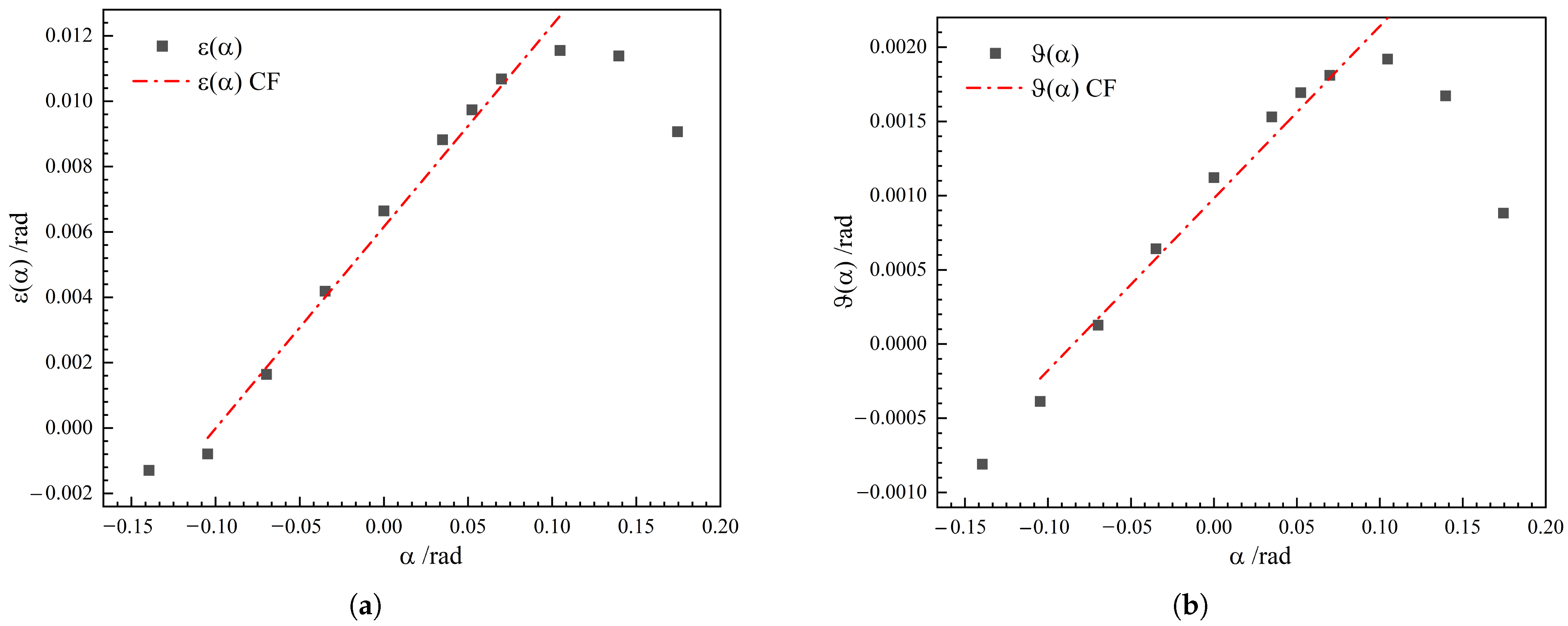
(2) The rear wing washout and front upwash gradient: Due to the downwash effect from the front wing, the lift force coefficient of the rear wing C L r w α is reduced compared to when the independently named C L r w s i α is considered, as shown in Figure A2a. The C L r w s i α is obtained by CFD simulation L 1 B . The downwash angle ε at the rear wing can be calculated for different angles of attack α , as illustrated in Figure A3a. By applying Equation (27) to determine the slope at various angles of attack, the gradient d ε d α is derived. A linear fitting over the angle of attack range [ 6 , 6 ] yields d ε d α = 0.0617 . Similarly, due to the upwash effect from the rear wing, the lift force coefficient of the front wing C L f w α is increased compared to when the independently named C L f w s i α is considered, as shown in Figure A2a. The upwash angle ϑ at the front wing for varying angles of attack α is shown in Figure A3b. By applying Equation (28), a linear fitting over the angle of attack range [ 6 , 6 ] yields d ϑ d α = 0.0115 .
(3) The dynamic pressure ratios: By performing measurements in Simulation L 1 , we can obtain Q = 545.85 Pa , Q f w = 535.34 Pa , and Q r w = 514.28 Pa , respectively. According to Equations (25) and (26), η f w = 0.98 and η r w = 0.98 .
Figure A2. The C L and C D curves for wings, and the C Y curve for the vertical tail. (a) The C L curve of the front and rear wing varies with α . (b) The C D curve of the front and rear wing varies with α . (c) The C Y curve of the vertical tail varies with β .
Drones 09 00231 g0a2
Figure A3. The rear wing downwash angle ε and the front wing upwash angle ϑ . (a) The rear wing downwash angle ε curve varies with α . (b) The front wing upwash angle ϑ curve varies with α .
Drones 09 00231 g0a3
Table A1. Three types of aerodynamic parameters.
ParameterValueParameterValue
C L 0 f w 0.58055 C D 0 r w 0.02183
C L α f w 5.95690 C D α f w 0.01
C L 0 r w 0.52586 C D α r w 0.085377
C L α r w 5.41630 C D α 2 f w 0.782014
C D 0 f w 0.01805 C D α 2 r w 0.946047
C Y β v t 0.27204 d ε d α 0.0617
d ϑ d α 0.0115 η r w 0.94
η f w 0.98 NANNAN

Appendix A.5. The Static and Control Derivatives CFD Simulation Results

Table A2. The static and control derivatives CFD simulation conditions.
NO. α ° β ° δ e ° δ a ° δ r °
L 1 8 , 16 0000
L 2 4 , 12 0 20 00
L 3 4 , 12 0 10 00
L 4 4 , 12 0 5 00
L 5 4 , 12 0500
L 6 4 , 12 01000
L 7 4 , 12 02000
S 1 4 , 0 , 4 , 8 20 , 15 , 10 000
S 2 4 , 0 , 4 , 8 00 20 0
S 3 4 , 0 , 4 , 8 00 15 0
S 4 4 , 0 , 4 , 8 00 10 0
S 5 4 , 0 , 4 , 8 000 20
S 6 4 , 0 , 4 , 8 000 15
S 7 4 , 0 , 4 , 8 000 10
Table A3. The coefficients varying with α .
α ° C L α C D α C m α
8 0.23638 0.05381 0.13286
6 0.08546 0.03837 0.15560
4 0.07525 0.03307 0.18571
2 0.25784 0.03293 0.20302
0 0.43081 0.03866 0.23285
2 0.59713 0.04962 0.25845
3 0.66783 0.05504 0.27648
4 0.75099 0.06497 0.32953
6 0.89351 0.07827 0.44741
8 1.00948 0.10006 0.58223
10 1.08601 0.11884 0.75643
12 1.08784 0.17252 1.03831
14 1.05311 0.23561 1.04370
16 1.00098 0.29398 0.89836
Table A4. The coefficients varying with β .
β ° C Y β C l β C n β Δ C D β
20 0.08153 0.00123 0.01046 0.028933
15 0.07312 0.00083 0.00832 0.016196
10 0.06091 0.00045 0.00621 0.005988
0 00 0.0061 0
10 0.06091 0.00045 0.00649 0.005988
15 0.07312 0.00083 0.00863 0.016196
20 0.08153 0.00123 0.01129 0.028933
Table A5. The coefficients varying with δ e .
δ e ° Δ C m δ e Δ C L δ e Δ C D δ e
20 1.6897 0.41838 0.008261
10 0.9787 0.22364 0.005241
5 0.4751 0.11904 0.003051
0 000
5 0.2356 0.07678 0.03577
10 0.6362 0.17078 0.020057
20 1.6419 0.3940 0.0578
Table A6. The coefficients varying with δ r .
δ r ° Δ C Y δ r Δ C l δ r Δ C n δ r
20 0.05040 0.00421 0.01560
15 0.04046 0.00382 0.01351
10 0.0345 0.00272 0.00675
0 000
10 0.03454 0.00272 0.00675
15 0.04046 0.00382 0.01351
20 0.05040 0.00421 0.01560
Table A7. The coefficients varying with δ a .
δ a ° Δ C l δ a Δ C n δ a
20 0.09466 0.00889
15 0.07829 0.00721
10 0.05456 0.000658
0 00
10 0.05456 0.000658
15 0.07829 0.00721
20 0.09466 0.00889

References

  1. Kryvokhatko, I.S. Aerodynamics of Tandem Wing Aircraft: From Dinosaurs to UAVs and Supersonic Planes; Springer: Berlin/Heidelberg, Germany, 2024. [Google Scholar]
  2. May, M.S.; Milz, D.; Looye, G. Semi-empirical aerodynamic modeling approach for tandem tilt-wing eVTOL control design applications. In Proceedings of the AIAA SciTech 2023 Forum, National Harbor, MD, USA, 23–27 January 2023. [Google Scholar] [CrossRef]
  3. Droandi, G.; Syal, M.; Bower, G. Tiltwing multi-rotor aerodynamic modeling in hover, transition and cruise flight conditions. In Proceedings of the 74th Annual Forum, AHS International Fairfax, Phoenix, AZ, USA, 14–17 May 2018; p. 1351. [Google Scholar] [CrossRef]
  4. Milz, D.; May, M.S.; Looye, G. Tandem tilt-wing control design based on sensory nonlinear dynamic inversion. In Proceedings of the AIAA AVIATION FORUM AND ASCEND 2024, Las Vegas, NV, USA, 29 July–2 August 2024; p. 4118. [Google Scholar] [CrossRef]
  5. Chauhan, S.S.; Martins, J.R.R.A. Tilt-Wing eVTOL Takeoff Trajectory Optimization. J. Aircr. 2020, 57, 93–112. [Google Scholar] [CrossRef]
  6. Puneet, S. Flight Dynamics and Control of the Butterfly eVTOL Aircraft in Hover. In Proceedings of the Vertical Flight Society’s 79th Annual Forum and Technology Display, West Palm Beach, FL, USA, 16–18 May 2023. [Google Scholar] [CrossRef]
  7. Munk, M.M. Elements of the Wing Section Theory and of the Wing Theory; US Government Printing Office: Washington, DC, USA, 1924; Volume 191.
  8. Voskuijl, M. Performance analysis and design of loitering munitions: A comprehensive technical survey of recent developments. Def. Technol. 2022, 18, 325–343. [Google Scholar] [CrossRef]
  9. Zhang, G.Q.; Yu, S.C.M. Unsteady aerodynamics of a morphing tandem-wing unmanned aerial vehicle. J. Aircr. 2012, 49, 1315–1323. [Google Scholar] [CrossRef]
  10. Liang, G.; Changle, L.; Hongzhe, J.; Yanhe, Z.; Jie, Z.; Hegao, C. Aerodynamic characteristics of a novel catapult launched morphing tandem-wing unmanned aerial vehicle. Adv. Mech. Eng. 2017, 9, 1687814017692290. [Google Scholar] [CrossRef]
  11. Broering, T.M.; Lian, Y.S. The effect of phase angle and wing spacing on tandem flapping wings. Acta Mech. Sin. 2012, 28, 1557–1571. [Google Scholar] [CrossRef]
  12. Scharpf, D.F.; Mueller, T.J. Experimental study of a low Reynolds number tandem airfoil configuration. J. Aircr. 1992, 29, 231–236. [Google Scholar] [CrossRef]
  13. Moschetta, J.M.; Thipyopas, C. Aerodynamic Performance of a Biplane Micro Air Vehicle. J. Aircr. 2007, 44, 291–299. [Google Scholar] [CrossRef]
  14. Faure, T.M.; Hétru, L.; Montagnier, O. Aerodynamic features of a two-airfoil arrangement. Exp. Fluids 2017, 58, 146. [Google Scholar] [CrossRef]
  15. Faure, T.M.; Dumas, L.; Montagnier, O. Numerical study of two-airfoil arrangements by a discrete vortex method. Theor. Comput. Fluid Dyn. 2020, 34, 79–103. [Google Scholar] [CrossRef]
  16. Kwiek, M.F.A. Analysis of longitudinal dynamic stability of tandem wing aircraft. Aircr. Eng. Aerosp. Technol. 2023, 95, 1411. [Google Scholar] [CrossRef]
  17. Goetzendorf-Grabowski, T. Flight dynamics of unconventional configurations. Prog. Aerosp. Sci. 2023, 137, 100885. [Google Scholar] [CrossRef]
  18. Gryte, K.; Hann, R.; Alam, M.; Roháč, J.; Johansen, T.A.; Fossen, T.I. Aerodynamic modeling of the Skywalker X8 Fixed-Wing Unmanned Aerial Vehicle. In Proceedings of the 2018 International Conference on Unmanned Aircraft Systems (ICUAS), Dallas, TX, USA, 12–15 June 2018; pp. 826–835. [Google Scholar] [CrossRef]
  19. Morelli, E.; Klein, V. Aircraft System Identification: Theory and Practice, 2nd ed.; Sunflyte Enterprises: Williamsburg, VA, USA, 2016. [Google Scholar]
  20. Simmons, B.M.; McClelland, H.G.; Woolsey, C.A. Nonlinear Model Identification Methodology for Small, Fixed-Wing, Unmanned Aircraft. J. Aircr. 2019, 56, 1056–1067. [Google Scholar] [CrossRef]
  21. Wang, Z.; Li, J.; Liu, C.; Yang, Y.; Li, J.; Wu, X.; Yang, Y.; Ye, B. Optimization-Assisted Filter for Flow Angle Estimation of SUAV Without Adequate Measurement. Drones 2024, 8, 758. [Google Scholar] [CrossRef]
  22. Pamadi, B. Performance, Stability, Dynamics, and Control of Airplanes, 2nd ed.; AIAA education series; American Institute of Aeronautics and Astronautics: Reston, VA, USA, 2004. [Google Scholar]
  23. Ronch, A.D.; Vallespin, D.; Ghoreyshi, M.; Badcock, K.J. Evaluation of dynamic derivatives using computational fluid dynamics. AIAA J. 2012, 50, 470–484. [Google Scholar] [CrossRef]
  24. Keller, J.B.; Rubinow, S.I. Slender-body theory for slow viscous flow. J. Fluid Mech. 1976, 75, 705–714. [Google Scholar] [CrossRef]
  25. Adams, M.C.; Sears, W.R. Slender-Body Theory-Review and Extension. J. Aeronaut. Sci. 1953, 20, 85–98. [Google Scholar] [CrossRef]
  26. Phillips, W.F.; Snyder, D.O. Modern Adaptation of Prandtl’s Classic Lifting-Line Theory. J. Aircr. 2000, 37, 662–670. [Google Scholar] [CrossRef]
  27. Landahl, M.T.; Stark, V.J.E. Numerical lifting-surface theory—Problems and progress. AIAA J. 1968, 6, 2049–2060. [Google Scholar] [CrossRef]
  28. Murua, J.; Palacios, R.; Graham, J.M.R. Applications of the unsteady vortex-lattice method in aircraft aeroelasticity and flight dynamics. Prog. Aerosp. Sci. 2012, 55, 46–72. [Google Scholar] [CrossRef]
  29. East, R.A.; Hutt, G.R. Comparison of predictions and experimental data for hypersonic pitching motion stability. J. Spacecr. Rocket. 1988, 25, 225–233. [Google Scholar] [CrossRef]
  30. Blake, W. Prediction of fighter aircraft dynamic derivatives using Digital Datcom. In Proceedings of the 3rd Applied Aerodynamics Conference, Colorado Springs, CO, USA, 14–16 October 1985. [Google Scholar] [CrossRef]
  31. Millard, J.; Booth, S.; Rawther, C.; Hayashibara, S. XFLR5 as a Design Tool in Remotely Controlled Design-Build-Fly Applications. In Proceedings of the AIAA SCITECH 2022 Forum, San Diego, CA, USA, 3–7 January 2022. [Google Scholar] [CrossRef]
  32. Melin, T. A Vortex Lattice MATLAB Implementation for Linear Aerodynamic Wing Applications. Master’s Thesis, Royal Institute of Technology, Stockholm, Sweden, 2000. [Google Scholar]
  33. Budziak, K. Aerodynamic Analysis with Athena Vortex Lattice (AVL); Aircraft Design and Systems Group (AERO), Department of Automotive and Aeronautical Engineering, Hamburg University of Applied Sciences: Hamburg, Germany, 2015. [Google Scholar] [CrossRef]
  34. McDonald, R.A.; Gloudemans, J.R. Open Vehicle Sketch Pad: An Open Source Parametric Geometry and Analysis Tool for Conceptual Aircraft Design. In Proceedings of the AIAA SCITECH 2022 Forum, San Diego, CA, USA, 3–7 January 2022. [Google Scholar] [CrossRef]
  35. Sooy, T.J.; Schmidt, R.Z. Aerodynamic Predictions, Comparisons, and Validations Using Missile DATCOM (97) and Aeroprediction 98 (AP98). J. Spacecr. Rocket. 2005, 42, 257–265. [Google Scholar] [CrossRef]
  36. Hui, W.H. Stability of oscillating wedges and caret wings in hypersonic and supersonic flows. AIAA J. 1969, 7, 1524–1530. [Google Scholar] [CrossRef]
  37. Hui, W.H.; Tobak, M. Bifurcation analysis of aircraft pitching motions about large mean angles of attack. J. Guid. Control Dyn. 1984, 7, 113–122. [Google Scholar] [CrossRef]
  38. Tobak, M.; Schiff, L.B. Generalized Formulation of Nonlinear Pitch-Yaw-Roll Coupling: Part I-Nonaxisymmetric Bodies. AIAA J. 1975, 13, 323–326. [Google Scholar] [CrossRef]
  39. Weinacht, P.; Sturek, W.B. Computation of the roll characteristics of a finned projectile. J. Spacecr. Rocket. 1996, 33, 769–775. [Google Scholar] [CrossRef]
  40. DeSpirito, J.; Silton, S.I.; Weinacht, P. Navier-Stokes Predictions of Dynamic Stability Derivatives: Evaluation of Steady-State Methods. J. Spacecr. Rocket. 2009, 46, 1142–1154. [Google Scholar] [CrossRef]
  41. Scott, R.C.; Pototzky, A.S. Quasisteady aerodynamics for flutter analysis using steady computational fluid dynamics calculations. J. Aircr. 1996, 33, 191–197. [Google Scholar] [CrossRef]
  42. Roy, J.F.L.; Morgand, S. SACCON CFD Static and Dynamic Derivatives Using elsA. In Proceedings of the 28th AIAA Applied Aerodynamics Conference, Chicago, IL, USA, 28 June–1 July 2010; p. 4562. [Google Scholar] [CrossRef]
  43. Mi, B.; Zhan, H.; Chen, B. New Systematic CFD Methods to Calculate Static and Single Dynamic Stability Derivatives of Aircraft. Math. Probl. Eng. 2017, 2017, 4217217. [Google Scholar] [CrossRef]
  44. Green, L.; Spence, A.; Murphy, P. Computational Methods for Dynamic Stability and Control Derivatives. In Proceedings of the 42nd AIAA Aerospace Sciences Meeting and Exhibit, Reno, NV, USA, 5–8 January 2004; p. 15. [Google Scholar] [CrossRef]
  45. Mi, B.; Zhan, H.; Chen, B. Calculating Dynamic Derivatives of Flight Vehicle with New Engineering Strategies. Int. J. Aeronaut. Space Sci. 2017, 18, 175–185. [Google Scholar] [CrossRef]
  46. Juliawan, N.; Chung, H.S.; Lee, J.W.; Kim, S. Estimation and Separation of Longitudinal Dynamic Stability Derivatives with Forced Oscillation Method Using Computational Fluid Dynamics. Aerospace 2021, 8, 354. [Google Scholar] [CrossRef]
  47. Hall, K.C.; Ekici, K.; Thomas, J.P.; Dowell, E.H. Harmonic balance methods applied to computational fluid dynamics problems. Int. J. Comput. Fluid Dyn. 2013, 27, 52–67. [Google Scholar] [CrossRef]
  48. Ronch, A.; McCracken, A.J.; Badcock, K.J.; Widhalm, M.; Campobasso, M.S. Linear Frequency Domain and Harmonic Balance Predictions of Dynamic Derivatives. J. Aircr. 2013, 50, 694–707. [Google Scholar] [CrossRef]
  49. Hassan, D.; Sicot, F. A Time-Domain Harmonic Balance Method for Dynamic Derivatives Predictions. In Proceedings of the 49th AIAA Aerospace Sciences Meeting including the New Horizons Forum and Aerospace Exposition, Orlando, FL, USA, 4–7 January 2011. [Google Scholar] [CrossRef]
  50. Murman, S.M. Reduced-Frequency Approach for Calculating Dynamic Derivatives. AIAA J. 2007, 45, 1161–1168. [Google Scholar] [CrossRef]
  51. Thomas, J.; Custer, C.; Dowell, E.; Hall, K. Unsteady Flow Computation Using a Harmonic Balance Approach Implemented About the OVERFLOW 2 Flow Solver. In Proceedings of the 19th AIAA Computational Fluid Dynamics, San Antonio, TX, USA, 22–25 June 2009; p. 4270. [Google Scholar] [CrossRef]
  52. Dimitriadis, G.; Panagiotou, P.; Dimopoulos, T.; Yakinthos, K. Prediction of aerodynamic loads and stability derivatives using the unsteady Source and Doublet Panel Method for preliminary aircraft design. In Proceedings of the AIAA SCITECH 2024 Forum, Orlando, FL, USA, 8–12 January 2024; p. 0239. [Google Scholar] [CrossRef]
  53. Gao, L.; Jin, H.; Zhao, J.; Cai, H.; Zhu, Y. Flight Dynamics Modeling and Control of a Novel Catapult Launched Tandem-Wing Micro Aerial Vehicle With Variable Sweep. IEEE Access 2018, 6, 42294–42308. [Google Scholar] [CrossRef]
  54. Wang, Z.; Xiong, J.; Cheng, X.; Li, J. Establishment and verification of longitudinal aerodynamic model of tandem wing aircraft. IOP Conf. Ser. Mater. Sci. Eng. 2019, 563, 032022. [Google Scholar] [CrossRef]
  55. Lua, K.B.; Lu, H.; Zhang, X.H.; Lim, T.T.; Yeo, K.S. Aerodynamics of two-dimensional flapping wings in tandem configuration. Phys. Fluids 2016, 28, 121901. [Google Scholar] [CrossRef]
  56. Beard, R.W.; McLain, T.W. Small Unmanned Aircraft: Theory and Practice; Princeton University Press: Princeton, NJ, USA, 2012. [Google Scholar]
  57. Stevens, B.L.; Lewis, F.L.; Johnson, E.N. Modeling the Aircraft; Chapter 2; John Wiley & Sons, Ltd.: Hoboken, NJ, USA, 2015; pp. 63–141. [Google Scholar] [CrossRef]
  58. Yang, Y.; Li, J.; Liu, C.; Yang, Y.; Li, J.; Wang, Z.; Wu, X.; Fu, L.; Xu, X. Automatic terminal guidance for small fixed-wing unmanned aerial vehicles. J. Field Robot. 2023, 40, 3–29. [Google Scholar] [CrossRef]
  59. Yang, Y.; Liu, C.; Li, J.; Yang, Y.; Li, J.; Zhang, Z.; Ye, B. Design, implementation, and verification of a low-cost terminal guidance system for small fixed-wing UAVs. J. Field Robot. 2021, 38, 801–827. [Google Scholar] [CrossRef]
  60. Mialon, B.; Khrabrov, A.; Khelil, S.B.; Huebner, A.; Da Ronch, A.; Badcock, K.; Cavagna, L.; Eliasson, P.; Zhang, M.; Ricci, S.; et al. Validation of numerical prediction of dynamic derivatives: The DLR-F12 and the Transcruiser test cases. Prog. Aerosp. Sci. 2011, 47, 674–694. [Google Scholar] [CrossRef]
  61. Ronch, A.D.; Ghoreyshi, M.; Badcock, K.; Vallespin, D. Computation and Evaluation of Dynamic Derivatives using CFD. In Proceedings of the 28th AIAA Applied Aerodynamics Conference, Chicago, IL, USA, 28 June–1 July 2010; p. 4817. [Google Scholar] [CrossRef]
  62. Shamsi, R.; Ghassemi, H. Time-Accurate Analysis of the Viscous Flow Around Puller Podded Drive Using Sliding Mesh Method. J. Fluids Eng. 2014, 137, 011101. [Google Scholar] [CrossRef]
  63. Belaidouni, H.; Samardžić, M.; Živković, S.; Kozić, M. Computational Fluid Dynamics and Experimental Data Comparison of a Missile Model Roll Derivative. J. Spacecr. Rocket. 2017, 54, 672–682. [Google Scholar] [CrossRef]
  64. Rizzi, A. Modeling and simulating aircraft stability and control—The SimSAC project. Prog. Aerosp. Sci. 2011, 47, 573–588. [Google Scholar] [CrossRef]
  65. Berndt, J. JSBSim: An open source flight dynamics model in C++. In Proceedings of the AIAA Modeling and Simulation Technologies Conference and Exhibit, Providence, RI, USA, 16–19 August 2004; p. 4923. [Google Scholar] [CrossRef]
  66. Berndt, J.; Marco, A.D. Progress On and Usage of the Open Source Flight Dynamics Model Software Library, JSBSim. In Proceedings of the AIAA Modeling and Simulation Technologies Conference, Chicago, IL, ISA, 10–13 August 2009; p. 5699. [Google Scholar] [CrossRef]
  67. Chicco, D.; Warrens, M.J.; Jurman, G. The coefficient of determination R-squared is more informative than SMAPE, MAE, MAPE, MSE and RMSE in regression analysis evaluation. Peerj Comput. Sci. 2021, 7, e623. [Google Scholar] [CrossRef]
Figure 1. The tandem-wing UAV configuration. (a) Vertical view. (b) Side view.
Drones 09 00231 g001
Figure 2. The effect of pitch rate on lift force.
Drones 09 00231 g002
Figure 3. The framework of dynamic derivative correction mechanism based on the CFD method.
Drones 09 00231 g003
Figure 4. The picture of SULA90.
Drones 09 00231 g004
Figure 5. The UAV surface mesh and dynamic mesh setting for longitudinal coupled dynamic derivatives simulations. (a) The mesh on the UAV surface and symmetry plane. (b) Dynamic mesh setup for longitudinal coupled dynamic derivative calculation.
Drones 09 00231 g005
Figure 6. The longitudinal harmonic oscillation simulation results of the whole UAV (from 2.1 s to 2.88 s). (a) The C L curve varies with time. (b) The C m curve varies with time. (c) The C D curve varies with time.
Drones 09 00231 g006
Figure 7. The longitudinal harmonic oscillation simulation results of the fuselage (from 2.1 s to 2.88 s). (a) The C L f u s curve varies with time. (b) The C m f u s curve varies with time. (c) The C D f u s curve varies with time.
Drones 09 00231 g007
Figure 8. The angular rate dynamic derivative curves. (a) The pitch angular rate derivatives curves vary with q ¯ . (b) The pitch angular rate derivative curves vary with p ¯ . (c) The roll angular rate derivatives curves vary with r ¯ .
Drones 09 00231 g008
Figure 9. The simulation models of XFLR5 and OpenVSP.
Drones 09 00231 g009
Figure 10. The framework of the open-loop model validation approach based on the field flight.
Drones 09 00231 g010
Figure 11. The main electrical components of SULA90.
Drones 09 00231 g011
Figure 12. The rectangular flight route.
Drones 09 00231 g012
Figure 13. The lateral-directional open-loop validation results. (a) The aileron control input δ a r e . (b) The prediction and flight record p.
Drones 09 00231 g013
Figure 14. The longitudinal open-loop validation results. (a) Throttle control PWM value. (b) The pitch control input δ e r e . (c) The prediction and flight record q.
Drones 09 00231 g014
Table 1. The main inertial and geometric properties of SULA90.
ParameterValue
Mass m12.8 kg
Body X b -axis moment of inertia J x x 0.510 kg/m2
Body Y b -axis moment of inertia J y y 1.739 kg/m2
Body Z b -axis moment of inertia J z z 2.073 kg/m2
Product of inertia about the X b and Z b axis J x z −0.018 kg/m2
Front wing span b f w 1.86 m
Rear wing span b r w 1.34 m
Vertical tail span b v t 0.3 m
Front wing chord c f w 0.113 m
Rear wing chord c r w 0.133 m
Vertical tail chord c v t 0.069 m
Front wing area S f w 0.21 m 2
Rear wing span S r w 0.17 m 2
Vertical tail span S v t 0.0514 m 2
Body length l b d 1 m
Front wing moment arm l f w 0.271 m
Rear wing moment arm l r w 0.540 m
Vertical tail moment arm l v t 0.468 m
Vertical tail chord c v t 0.069 m
Vertical distance of vertical tail z v t 0.15 m
Aileron control input δ a and deflection angle 1 , 1 , 30 , 30 deg
Elevator control input δ e and deflection angle 1 , 1 , 30 , 30 deg
Rudder control input δ r and deflection angle 1 , 1 , 30 , 30 deg
Table 2. The CFD simulation longitudinal dynamic derivatives.
ParameterValueParameterValueParameterValue
C L α ˙ + C L q 14.2575 C L q 12.8540 C L α ˙ 1.4035
C m α ˙ + C m q 136.5106 C m q 134.1540 C m α ˙ 2.3566
C D α ˙ + C D q 1.5176 C D q 1.3421 C D α ˙ 0.1755
C L α ˙ f u s + C L q f u s 2.0445 C L q f u s 1.8395 C L α ˙ 0.2050
C m α ˙ f u s + C m q f u s 3.8531 C m q f u s 3.634 C m α ˙ 0.2191
C D α ˙ f u s + C D q f u s 0.4619 C D q f u s 0.4228 C D α ˙ 0.0391
Table 3. Dynamic derivative accuracy criteria [30].
ParameterOpen LoopClosed Loop
C * q * = L , D , m 25 % 50 %
C * α ˙ * = L , D , m 25 % 50 %
C l p 0.5 /rad 0.2 /rad
C n p 0.05 /rad 0.2 /rad
C l r 0.1 /rad 0.2 /rad
C n r 0.1 /rad 0.2 /rad
Table 4. The dynamic derivatives of different methods.
Param.CFDCEHMADRD %XFLR5ADRD %OpenVSPADRD %
C L q 11.0145 12.157 1.14 10.37 14.245 3.231 29.33 14.058 3.044 27.63
C m q 130.52 136.541 6.021 4.61 148.24 17.720 13.58 146.050 15.530 11.90
C D q 0.9193 0.7321 0.187 20.36 NANNANNAN 0.4771 0.442 48.10
C L α ˙ 1.1985 1.5819 0.383 31.99 NANNANNANNANNANNAN
C m α ˙ 2.1375 3.7354 1.598 74.76 NANNANNANNANNANNAN
C Y r 0.6888 0.448 0.241 34.96 0.1211 0.568 82.42 0.1170 0.572 83.01
C l p 0.7513 0.6371 0.114 15.20 0.49469 0.257 34.16 0.4997 0.252 33.49
C l r 0.5491 0.3668 0.182 33.20 0.12706 0.422 76.86 0.1128 0.436 79.46
C n p 0.1106 0.0891 0.022 19.44 0.06131 0.049 44.57 0.05025 0.060 54.57
C n r 0.22131 0.116 0.105 47.58 0.02977 0.192 86.55 0.03737 0.184 83.11
Disclaimer/Publisher’s Note: The statements, opinions and data contained in all publications are solely those of the individual author(s) and contributor(s) and not of MDPI and/or the editor(s). MDPI and/or the editor(s) disclaim responsibility for any injury to people or property resulting from any ideas, methods, instructions or products referred to in the content.