Positioning Error Analysis of Distributed Random Array Based on Unmanned Aerial Vehicles in Collaborative Jamming

Abstract

Distributed beamforming has emerged as a pivotal technology in modern communication systems, radar applications, and collaborative electronic warfare. Through distributed collaboration, these jamming nodes composed of unmanned aerial vehicles (UAVs) can execute flexible electronic jamming toward wireless communication systems despite energy limitations. However, they encounter challenges such as time and positioning inaccuracies, which can diminish the synthesis power of jamming beams and reduce jamming effectiveness. This paper examines the impact of angle and distance errors on jamming effectiveness, deriving upper error bounds under various suppression coefficients. The findings offer practical guidelines for enhancing the precision and effectiveness of distributed beamforming systems in electronic warfare applications.

1. Introduction

Artificial intelligence and information technologies are revolutionizing combat styles, making electronic warfare (EW) a central component of intelligent warfare [1,2,3]. Collaborative electronic warfare, leveraging swarm intelligence, has emerged as a key research focus globally [4,5,6,7,8,9,10]. Traditional EW systems rely on phased arrays or ground-based high-power jammers [11,12], which, while ensuring array coherence and strong suppression, suffer from limited flexibility and poor adaptability to dynamic operations.

The low cost, high mobility, and rapid deployment of UAVs have been widely applied in intelligent warfare, and these collaborative UAVs are usually called swarms. These swarms utilize distributed collaborative beamforming technology for precise electronic jamming [13,14]. However, unlike phased arrays and traditional ground jamming systems, swarm-based distributed arrays face significant challenges in achieving precise time and phase synchronization. As the UAVs are distributed in the air, the jamming waveforms arrive at the target area asynchronously. Moreover, UAV positioning accuracy is affected by both wind-induced jitter and GPS errors, potentially degrading beamforming performance. Fortunately, the time error can be mitigated through closed-loop or open-loop compensation techniques [15,16,17]. However, in the real world, the UAVs’ jitter and GPS errors are irresistible factors that limit the jamming performance. Therefore, it is essential to analyze the positioning errors. In different tasks, a reasonable positioning accuracy is determined according to the upper bounds of the errors, so the jamming effect can be guaranteed and the cost can be saved.

There is considerable research on evaluating beamforming effects, error analysis, and node synchronization in distributed beamforming. The millimeter-wave and MIMO phased array antennas were examined in 5G/6G networks [18]. The paper highlighted beamforming integration, addressing benefits, challenges, and security for automotive systems, smart cities, and IoT while exploring future advancements. A gain calculation model for distributed beamforming was developed within a two-level beamforming topology [19,20,21,22], where the array elements are composed of omnidirectional antennas. They analyzed the error limits for achieving 90% gain under different node counts. The authors in [23] have studied the development of beamforming technology over the past 25 years, addressing both convex and non-convex optimization challenges. The study employed the signal-to-interference-plus-noise ratio (SINR) as a key performance metric, revealing that even minor synchronization errors can significantly degrade SINR performance. Positioning errors, including both angular and distance errors, directly affect the node phase alignment, hindering coherent waveform superposition at the target location. Therefore, after considering all contributing factors, the effect of phase errors on beamforming was analyzed [24]. The article discusses the influence of phase error percentage (PEP) on the bit error rates (BERs) and signal-to-noise ratio (SNR) across various signal types, including multi-tone and broadband signals, in a system where omnidirectional antennas are employed as array elements. Conventional beamforming (CBF) is a fixed beamforming method that can control beam direction by adjusting node weights, requiring less power consumption and fewer computational resources. However, its performance degrades in complex electronic countermeasure environments. In contrast, adaptive beamforming techniques, particularly the minimum variance distortionless response (MVDR) method [25], demonstrate superior performance. The MVDR optimizes beamforming by minimizing output power variance, achieving enhanced robustness and deeper nulls (up to 30 dB improvement) compared to CBF in similar operational scenarios. Phase uncertainty directly leads to errors in the steering vector (SV). A reconstruction algorithm was proposed for the interference-plus-noise covariance matrix (IPCM) [26]: analyzing the relationship between the correlation degree and error magnitude among nodes in the generated SV dataset with positioning errors, the authors estimated positioning errors based on a weighted subspace fitting algorithm. The reconstructed IPCM showed better beam performance. Even when the errors reached half the node distribution radius, the SINR would only degrade by 4 dB, significantly enhancing stability. A method for optimizing phase delay was designed in a smart MIMO antenna system [27], enabling precise beam steering and high directional gain for future wireless networks. The design employs phase shifters to enhance power efficiency and reduce interference. In terms of physical-layer security, the authors in [28] proposed a hybrid beamforming and jamming scheme to secure a two-way relay network against eavesdropping. It combines signal relaying and jamming under individual power constraints. An efficient algorithm outperforms conventional methods, validated by numerical results. Recent studies have advanced our understanding of positioning errors in distributed antenna systems. The authors in [29] investigated a random array of omnidirectional antennas distributed on a spherical space, developing analytical models for average radiated power and array factor in Cartesian and spherical coordinate systems. Their work established probability distribution functions for beam characteristics under various error conditions. Positioning errors were also analyzed in sparse arrays [30], quantifying their impact by analyzing the cumulative distribution function and peak power under different positioning errors.

The development of collaborative jamming has been significantly advanced by multi-agent system research, driving large-scale jammers toward miniaturization and multi-node configurations. This evolution enables more flexible and scalable electronic warfare capabilities, marking a critical shift in jamming system design and deployment. Compared with ground jammers and phased arrays, UAVs offer superior flexibility in jamming source deployment and can operate closer to targets, while their distributed architecture significantly enhances operational survivability [31,32]. In the context of low-altitude security, literature [33] proposed a distributed jamming strategy for UAV swarms. In a UAV jamming model based on satellite navigation, the tabu search artificial bee colony algorithm was utilized to optimize the distribution strategy of jamming nodes, achieving efficient collaborative jamming. In cognitive communications, jamming techniques have been effectively adapted for eavesdropper suppression to enhance communication security [34,35]. Addressing the complex challenges of jamming optimization, Tao et al. proposed an alternative optimization algorithm to address the non-convex joint optimization problem during the jamming process, which enhances the jamming effect [36].

Previous studies mainly calculated the beam power ratio at the target location under ideal conditions to that under conditions with errors. This power ratio metric is a key gain indicator for assessing positioning error effects in distributed beamforming systems. The application scenarios focused on multiple-input multiple-output (MIMO) communication, evaluating communication quality using parameters such as SNR and BER. Most collaborative algorithms focused on point-to-point jamming and did not model swarm as a target. However, in collaborative jamming, it is essential to consider not only the characteristics of the beam itself but also the power distribution in the target area and the size of the effective jamming region. Therefore, the performance evaluation method for point beams is unsuitable for analyzing jamming efficiency. In addition to considering the array directivity, it is necessary to consider the distribution of the jamming beam after transmission to the target area and the effective coverage range.

Under limited accuracy in directional and distance measurement conditions, errors in both direction and distance will be introduced. This paper systematically investigates how these errors affect the jamming-to-signal ratio (JSR) and the effective jamming range. Furthermore, the positional accuracy requirements are calculated based on varying nodes and distribution radius numbers. The main contributions of this study are as follows:

• A calculation method for the jamming gain is proposed based on the pattern multiplication theorem and radiation intensity, further researching the power propagation in the target area, no longer limited to the characteristics of the beam itself.
• The target azimuth JSR and effective jamming range are defined as performance evaluation parameters based on collaborative jamming scenarios, which are more matched with jamming scenarios compared to analyzing the half-power beamwidth (HPBW) and power of the array’s main lobe.
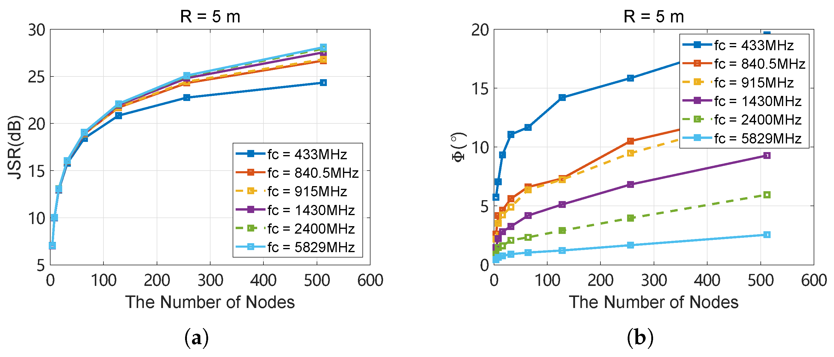
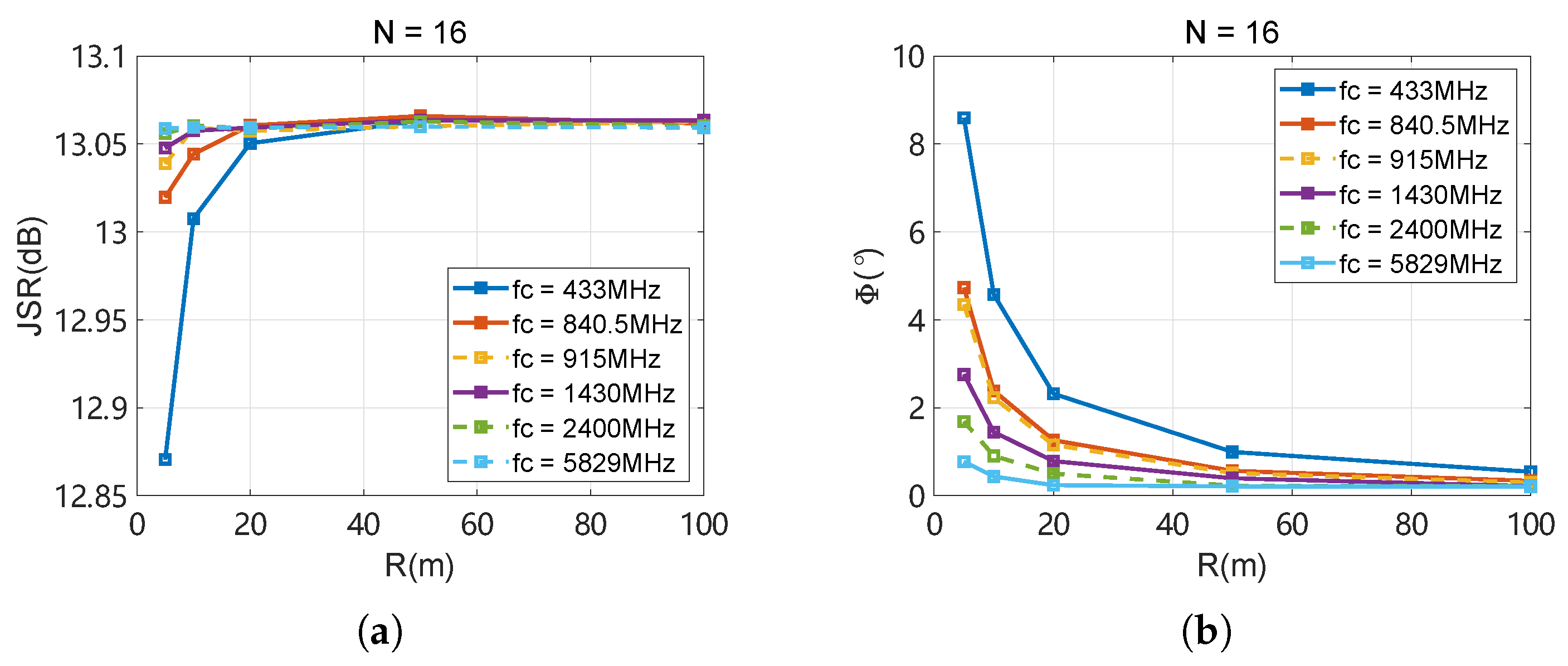
• The trend of JSR and effective range changes at different jamming frequencies is simulated under various distribution radii and numbers of nodes.
• The upper bounds of azimuth and distance errors are provided in multiple collaborative jamming scenarios where the effective jamming probability reaches 90%.
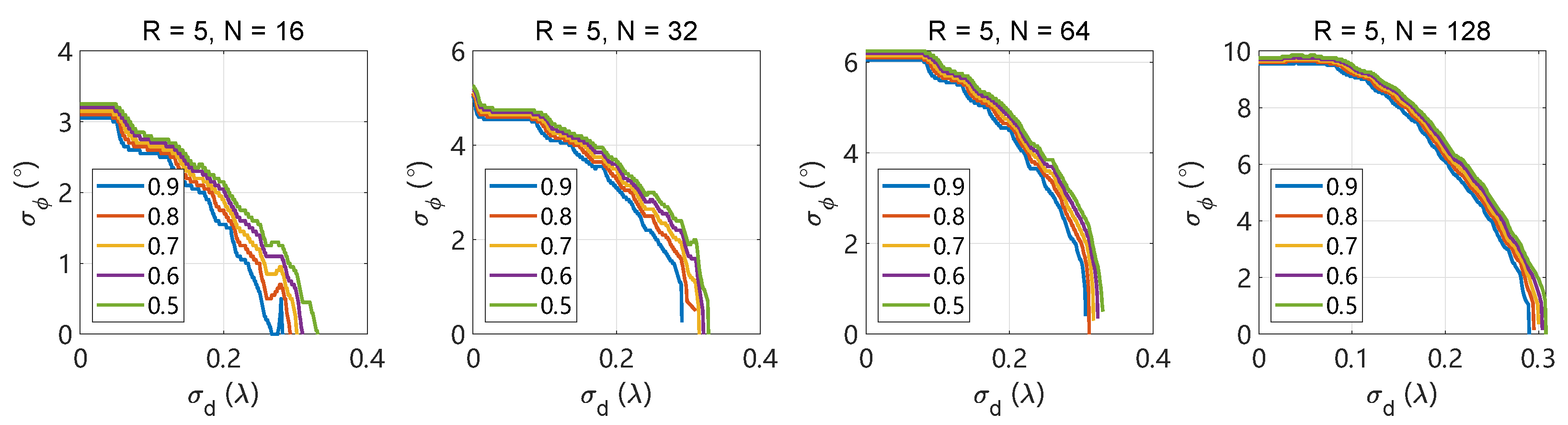
• The inter-relationship between azimuth and distance errors is analyzed under different effective jamming probabilities, providing a reference for rationally selecting the number of nodes and deploying swarms.

The rest of this paper is arranged as follows. Section 2 derives the far-field condition applicable to distributed arrays. Section 3 extracts the JSR formula for the array and presents a model for the jamming power transmission in free space. In Section 4, the target JSR and the effective jamming range are proposed to assess the jamming efficiency, and the effect of azimuth and distance errors on the metrics is discussed. Section 4.2.3 conducts comprehensive experiments based on real-world scenarios to validate the combined effects of the azimuth error and distance error, whereas Section 6 concludes this paper.

2. The Far-Field Condition

The UAVs are randomly distributed within a spherical space with radius R, as illustrated in Figure 1. Each UAV acts as a node equipped with an omnidirectional antenna. The position of each node is defined by spherical coordinates $(r_k,{\theta }_k,{\varphi }_k)$, where $r_k$ is the distance from the center of the spherical space, ${\theta }_k$ is the polar angle, and ${\varphi }_k$ is the azimuthal angle. The omnidirectional antennas enable uniform signal radiation or reception in all directions, allowing the system to synthesize a directed beam toward the target by controlling the phase and amplitude of each node’s signal. This spherical distribution of UAV nodes provides flexibility for three-dimensional beamforming, enhancing adaptability and coverage in dynamic environments. As a result, a directional beam is formed at the target location $(L,{\varphi }_0,{\theta }_0)$.

The distance $d_k$ between the node k and any point of space is given by

$$d_k=\sqrt{{(x_k-x)}^2+{(y_k-y)}^2+{(z_k-z)}^2}$$

(1)

The transformation between polar coordinates and the Cartesian coordinate system is

$$\left\{\begin{array}{cc}x=Lsin\left(\theta \right)cos\left(\varphi \right),\hfill & x_k=r_{k}sin\left({\theta }_k\right)cos\left({\varphi }_k\right)\hfill \\ y=Lsin\left(\theta \right)sin\left(\varphi \right),\hfill & y_k=r_{k}sin\left({\theta }_k\right)sin\left({\varphi }_k\right)\hfill \\ z=Lcos\left(\theta \right),\hfill & z_k=r_{k}cos\left({\theta }_k\right)\hfill \end{array}\right.$$

(2)

Bringing Equation (2) into Equation (1), $d_k$ can be written as

$$\begin{array}{cc}\hfill d_k& =\sqrt{L^2+r_k^2-2r_{k}L(sin\theta sin{\theta }_{k}cos(\varphi -{\varphi }_k)+cos\theta cos{\theta }_k)}\hfill \\ \hfill & =L\sqrt{1+{\displaystyle \frac{r_k^2}{L^2}}-{\displaystyle \frac{2r_k}{L}}\left(sin\theta sin{\theta }_{k}cos(\varphi -{\varphi }_k)+cos\theta cos{\theta }_k\right)}\hfill \end{array}$$

(3)

The first-order expansion of the Taylor series is $\sqrt{1+x}\approx 1+{\displaystyle \frac{x}{2}}$, so Equation (3) can continue to be reduced to

$$\begin{array}{cc}\hfill \widetilde{d_k}& \approx L\left(1+{\displaystyle \frac{1}{2}}\left({\displaystyle \frac{r_k^2}{L^2}}-{\displaystyle \frac{2r_k}{L}}\left(sin\theta sin{\theta }_{k}cos(\varphi -{\varphi }_k)+cos\theta cos{\theta }_k\right)\right)\right)\hfill \\ \hfill & \approx L+{\displaystyle \frac{r_k^2}{2L}}-r_k\left[sin\theta sin{\theta }_{k}cos(\varphi -{\varphi }_k)+cos\theta cos{\theta }_k\right]\hfill \end{array}$$

(4)

Under the far-field condition, where $L\gg r_k$, the term $r_k^2/2L$ in Equation (4) can be neglected. Thus, the final expression for $\widetilde{d_k}$ is written as

$$\widetilde{d_k}\approx L-r_k\left[sin\theta sin{\theta }_{k}cos(\varphi -{\varphi }_k)+cos\theta cos{\theta }_k\right]$$

(5)

To further quantify the far-field condition, the difference between $d_k$ and $\widetilde{d_k}$ is calculated:

$$\begin{array}{cc}\hfill \mathrm{\Delta }{d}_k& =d_k-\widetilde{d_k}\hfill \\ \hfill & =L\sqrt{1+{\displaystyle \frac{r_k^2}{L^2}}-{\displaystyle \frac{2r_k}{L}}\left(sin\theta sin{\theta }_{k}cos(\varphi -{\varphi }_k)+cos\theta cos{\theta }_k\right)}\hfill \\ \hfill & -L+r_k\left[sin\left(\theta \right)sin\left({\theta }_k\right)cos(\varphi -{\varphi }_k)+cos\left(\theta \right)cos\left({\theta }_k\right)\right]\hfill \end{array}$$

(6)

With the Taylor series, Equation (6) is written as

$$\begin{array}{cc}\hfill \mathrm{\Delta }{d}_k& \approx {\displaystyle \frac{r_k^2-2L{r}_k\left[sin\left(\theta \right)sin\left({\theta }_k\right)cos(\varphi -{\varphi }_k)+cos\left(\theta \right)cos\left({\theta }_k\right)\right]}{2L}}\hfill \\ \hfill & +r_k\left[sin\left(\theta \right)sin\left({\theta }_k\right)cos(\varphi -{\varphi }_k)+cos\left(\theta \right)cos\left({\theta }_k\right)\right]\hfill \\ \hfill & ={\displaystyle \frac{r_k^2}{2L}}\hfill \end{array}$$

(7)

Since the nodes are distributed in a sphere of radius R, the maximum value of $r_k$ can be written as

$$r_k^{\max }=R^2$$

(8)

Thus, the maximum value of $\mathrm{\Delta }{d}_k$ is given by

$$\mathrm{\Delta }{d}_k^{\max }={\displaystyle \frac{{\left(r_k^{\max }\right)}^2}{2L}}={\displaystyle \frac{R^2}{2L}}$$

(9)

Usually, in distributed beamforming, the upper limit of $\mathrm{\Delta }{d}_k$ needs to be less than half of the jamming wavelength to meet the far-field condition and form a plane wave in the target area. Thus, the relationship between R and L can be expressed as

$${\displaystyle \frac{R^2}{2L}}\le 0.5\lambda$$

(10)

where $\lambda$ is the wavelength of the jamming wave. The far-field condition is considered to be met when the distribution range of the array R is less than $\sqrt{L\lambda }$. The upper bounds of R under different $\lambda$ are shown in Figure 2, the frequency range corresponding to $\lambda$ is 433–5829 MHz, and the minimum value of R is $4.53\mathrm{m}$ in all results, which meets the spacing requirements for the safe flight of UAVs [30].

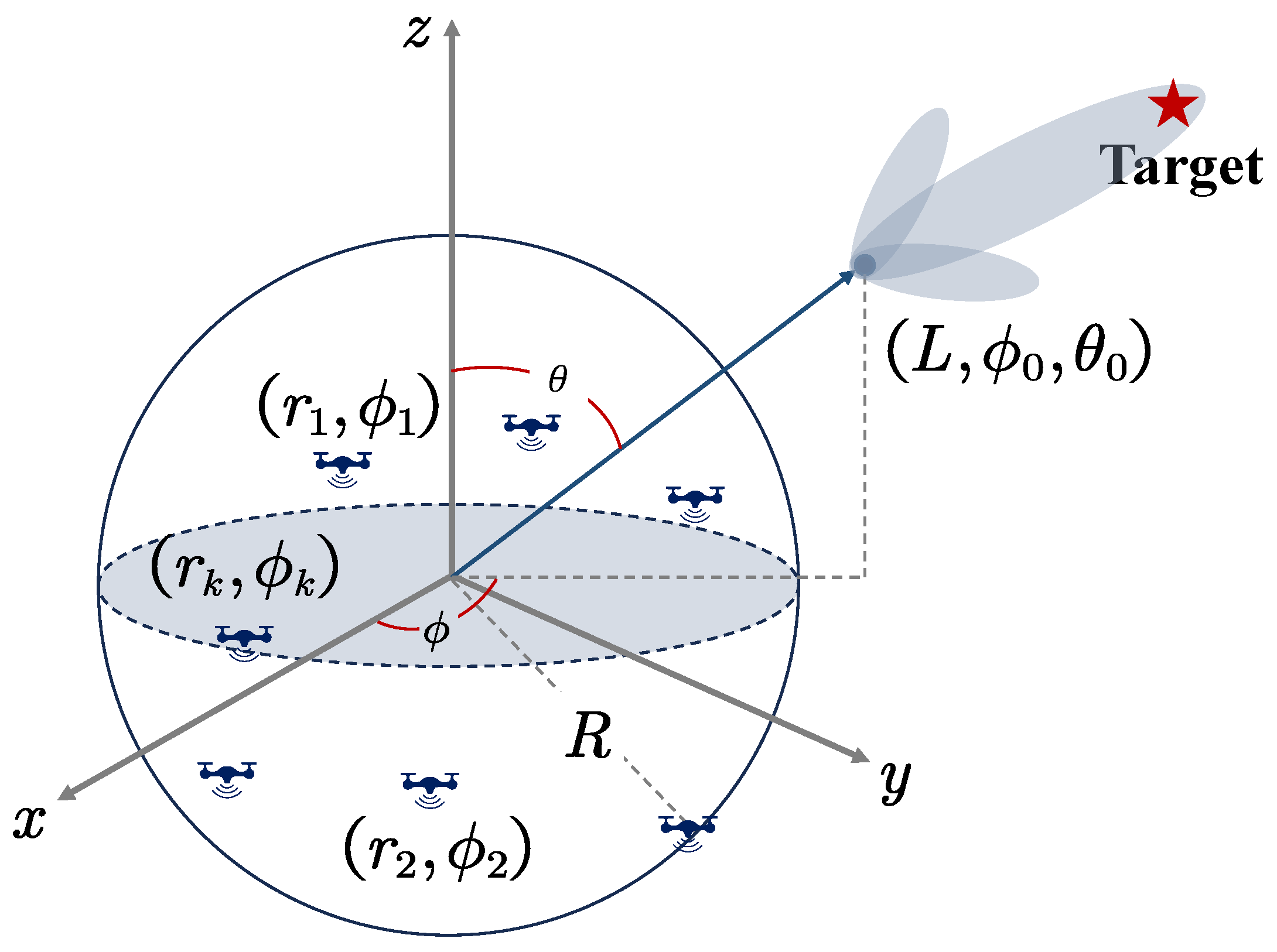
3. Collaborative Jamming Model

The array factor of the distributed jamming array is defined as

$$F(\theta ,\varphi )=\sum _{k=0}^{N-1}{e}^{j{\phi }_k}{e}^{j{\displaystyle \frac{2\pi }{\lambda }}{d}_k(\theta ,\varphi )}$$

(11)

where ${\phi }_k$ is the initial phase of node k, which can be calculated from $d_k$:

$${\phi }_k=-{\displaystyle \frac{2\pi }{\lambda }}{d}_k({\theta }_0,{\varphi }_0)$$

(12)

According to the pattern multiplication theorem, the pattern $B(\theta ,\varphi )$ of the array is equal to the product of the array factor and the element-normalized pattern $f(\theta ,\varphi )$, so $B(\theta ,\varphi )$ can be written as the following [37]:

$$B(\theta ,\varphi )=f(\theta ,\varphi )·F(\theta ,\varphi )$$

(13)

The directivity of the array is defined as the ratio of the radiation intensity in a given direction to the radiation intensity of an isotropic antenna with the same total radiation power, which is given by

$$D(\theta ,\varphi )={\displaystyle \frac{U_{rad}(\theta ,\varphi )}{U_{rad}^{iso}}}$$

(14)

where $U_{rad}(\theta ,\varphi )$ is the radiant intensity in the direction of $(\theta ,\varphi )$, and $U_{rad}^{iso}$ is the radiant intensity of an isotropic radiator, which is the total transmitted power divided by the solid angle of a sphere $4\pi$:

$$U_{rad}^{iso}={\displaystyle \frac{P_{total}}{4\pi }}$$

(15)

where $P_{total}$ is the total radiated power from the array, which is calculated by the integral of $B(\theta ,\varphi )$ on the sphere:

$$P_{total}={\int }_0^{2\pi }{\int }_0^{\pi }{\left|B(\theta ,\varphi )\right|}^{2}sin\theta d\theta d\varphi$$

(16)

Therefore, the directivity of the array can be written as

$$D(\theta ,\varphi )=4\pi {\displaystyle \frac{{\left|B(\theta ,\varphi )\right|}^2}{{\int }_0^{2\pi }{\int }_0^{\pi }{\left|B(\theta ,\varphi )\right|}^{2}sin\theta d\theta d\varphi }}$$

(17)

The multiplication of directivity and efficiency factor ($0\le \eta \le 1$) is the gain of the array:

$$G(\theta ,\varphi )=\eta ·D(\theta ,\varphi )$$

(18)

According to the one-way free-space propagation model, the uplink power $P_{rs}$ and jamming power at target $P_{rj}$ are written as

$$\left\{\begin{array}{c}{P}_{rs}={\displaystyle \frac{P_{ts}·G_{ts}·G_{rs}·{\lambda }^2}{{\left(4\pi d_c\right)}^2}}\hfill \\ P_{rj}={\displaystyle \frac{P_{tj}·G_{tj}·G_{rs}·{\lambda }^2}{{\left(4\pi d_j\right)}^2}}\hfill \end{array}\right.$$

(19)

where $P_{ts}$ is the transmitted power from the target’s base station, $P_{tj}$ is the transmitted power of the jamming swarms, $G_{ts}$ and $G_{tj}$ are the antennas of the base station and jamming swarms, respectively, and $G_{rs}$ is the target’s antenna. $d_c$ is the distance between the target and its base station and $d_j$ is the distance between the jamming array and the target. According to Equation (19), $JSR$ can be written as

$$JSR(\theta ,\varphi )={\displaystyle \frac{P_{rj}}{P_{rs}}}={\displaystyle \frac{P_{tj}·G_{tj}}{P_{ts}·G_{ts}}}·{\left[{\displaystyle \frac{d_c}{d_j}}\right]}^2$$

(20)

This paper mainly compares the influence of positioning errors on jamming power. In order to simplify the operation and avoid the influence of other factors, the antenna of the base station is set to be an isotropic antenna, namely $G_{ts}=1$, and the simplified expression is

$$\begin{array}{cc}\hfill JSR(\theta ,\varphi )& ={\displaystyle \frac{P_{tj}·G_{tj}}{P_{ts}}}·{\left[{\displaystyle \frac{d_c}{d_j}}\right]}^2\hfill \\ \hfill & ={\displaystyle \frac{\eta P_{tj}{D}_{tj}}{P_{ts}}}·{\left[{\displaystyle \frac{d_c}{d_j}}\right]}^2\hfill \\ \hfill & ={\displaystyle \frac{{4\pi \left|B(\theta ,\varphi )\right|}^2}{{\int }_0^{2\pi }{\int }_0^{\pi }{\left|B(\theta ,\varphi )\right|}^{2}sin\theta d\theta d\varphi }}·\mathcal{P}\hfill \end{array}$$

(21)

where

$$\mathcal{P}=\eta {\displaystyle \frac{P_{tj}}{P_{ts}}}·{\left[{\displaystyle \frac{d_c}{d_j}}\right]}^2$$

(22)

Since nodes are all isotropic antennas, assume that $f(\theta ,\varphi )=1$, and $\theta$ has the same characteristic with $\varphi$, and assume that $\theta ={\theta }_k={\theta }_0=\pi /2$. Based on Equations (5) and (11), $JSR(\theta ,\varphi )$ is rewritten as

$$JSR\left(\varphi \right|\theta ={\theta }_0)={\displaystyle \frac{4\pi N^2}{{\int }_0^{2\pi }{\int }_0^{\pi }{\left|B(\theta ,\varphi )\right|}^{2}sin\theta d\theta d\varphi }}·\mathcal{P}$$

(23)

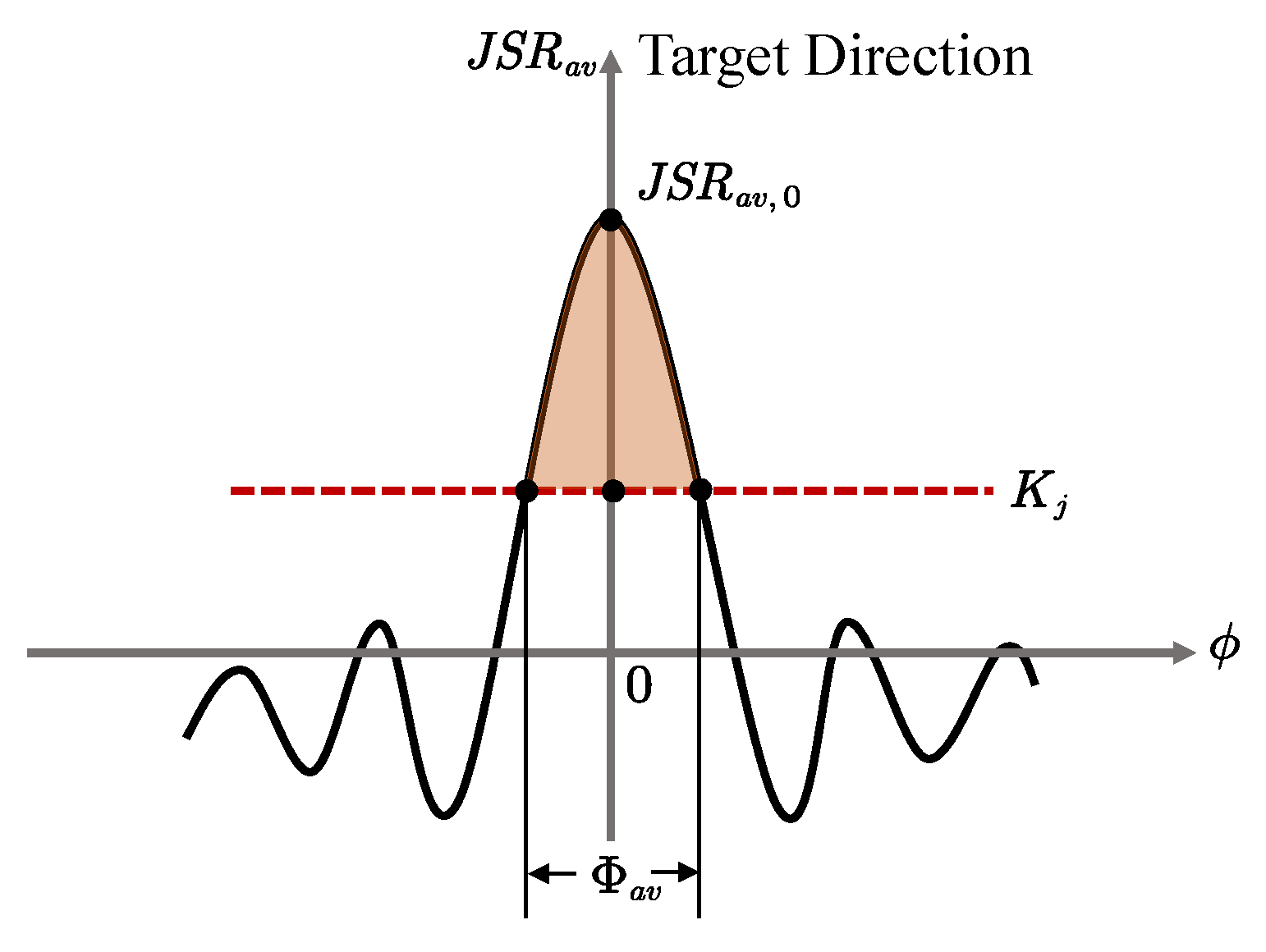
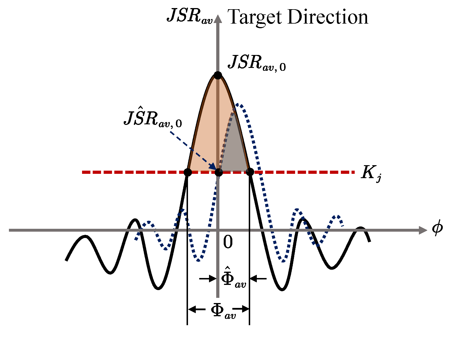
4. Jamming Effectiveness Evaluation

According to the result in Appendix A, the average of $JSR\left(\varphi \right|\theta ={\theta }_0)$ is given by

$$\begin{array}{cc}\hfill JS{R}_{av}& ={\displaystyle \frac{4\pi N^2}{{\int }_0^{2\pi }{\int }_0^{\pi }\mathbb{E}\left[{\left|B(\theta ,\varphi )\right|}^2\right]sin\theta d\theta d\varphi }}·\mathcal{P}\hfill \\ \hfill & ={\displaystyle \frac{N\mathcal{P}}{1+(N-1)T_1}}\hfill \end{array}$$

(24)

where

$$\begin{array}{cc}\hfill & T_1={\displaystyle \frac{2}{5}}\left({}_1{F}_2\left[{\displaystyle \frac{1}{2}};4,{\displaystyle \frac{7}{2}};-{\displaystyle \frac{x^2}{4}}\right]-6\times {}_1{F}_2\left[{\displaystyle \frac{1}{2}};3,{\displaystyle \frac{7}{2}};-{\displaystyle \frac{x^2}{4}}\right]\right)\hfill \\ \hfill & x=8\pi R/\lambda \hfill \end{array}$$

(25)

where ${}_1{F}_2$ is the generalized hypergeometric function. Figure 3 represents the spatial distribution of $JS{R}_{av}$, and $JS{R}_{av,0}$ is calculated with ${\varphi }_0=0$. $K_j$ is the jamming suppression factor, which is set according to different targets and conditions. Once $JS{R}_{av}>K_j$, the jamming effect is considered to be effective. The range of $\varphi$ corresponding to the effective jamming interval is called the effective jamming range, which is defined as ${\mathrm{\Phi }}_{av}$. In Appendix B, it is shown that

$${\mathrm{\Phi }}_{av}=2{\varphi }_{av}^{valid}=2arcsin{\displaystyle \frac{\lambda \mathcal{X}}{4\pi }}$$

(26)

Therefore, this paper proposes $JS{R}_{av,0}$ and ${\mathrm{\Phi }}_{av}$ as the metrics for jamming success.

4.1. Ideal Jamming Effectiveness

In order to verify the rationality of $JS{R}_{av,0}$ and ${\mathrm{\Phi }}_{av}$, under ideal conditions, $P_{tj},P_{ts},d_j$, and $d_c$ remain unchanged. The variation trends of $JS{R}_{av,0}$ and ${\mathrm{\Phi }}_{av}$ under different distribution radii R, numbers of nodes N, and carrier frequencies $f_c$ are compared. Firstly, since $R=5$ m, the effects of N on $JS{R}_{av,0}$ and ${\mathrm{\Phi }}_{av}$ are compared. As depicted in Figure 4a, an increase in N leads to a greater superposition of energy in the target area, resulting in a rise in $JS{R}_{av,0}$. As N escalates from 4 to 100, $JS{R}_{av,0}$ experiences a marked improvement. This enhancement is more pronounced at the higher frequencies, where the change rate of $JS{R}_{av,0}$ outpaces that of the lower frequencies. Consequently, for any given N, $JS{R}_{av,0}$ is higher at the higher frequencies. This trend can be attributed to the shorter wavelengths of the high-frequency jamming wave, resulting in a more concentrated energy distribution and lower transmission loss. In terms of the effective jamming range ${\mathrm{\Phi }}_{av}$, there are lower values in ${\mathrm{\Phi }}_{av}$ across different frequencies with fewer nodes, as shown in Figure 4b. However, as N increases, ${\mathrm{\Phi }}_{av}$ at the lower frequencies surpasses that of the higher frequencies. This phenomenon is directly related to the wavelength of the jamming signal. The lower frequencies correspond to longer wavelengths, which tend to spread out more, thus covering a larger area. In essence, while the high-frequency signals provide a more concentrated jamming effect, the low-frequency signals offer a broader jamming range. The balance between concentrated energy delivery and broader coverage should be carefully managed to optimize jamming systems for specific applications. Increasing N is crucial for enhancing $JS{R}_{av,0}$ for low-frequency operations, ensuring a robust jamming signal at the target. For high-frequency operations, N is pivotal in expanding ${\mathrm{\Phi }}_{av}$, allowing the jamming signal to cover a larger area effectively.

Secondly, when N is 16, $JS{R}_{av,0}$ and ${\mathrm{\Phi }}_{av}$ versus R is compared. As shown in Figure 5a, R increases to 20 m, $JSR$ will increase, and the growth of the low frequency is more significant than at the high frequency. This trend can be attributed to the fact that, when the node spacing is too small, the distributed array’s main lobe enlarges, preventing the energy from being well concentrated. In addition, at the same R, $JS{R}_{av,0}$ of the high frequency is larger due to the shorter wavelengths, which allow for a more focused beam, thus achieving a higher $JS{R}_{av,0}$. When R is greater than 20 m, the beam synthesis efficiency of the array will be saturated, so $JS{R}_{av,0}$ will hardly change regardless of further increases in R. This saturation occurs because the array no longer satisfies the far-field condition necessary for the array to maintain a focused beam. As a result, the energy cannot be further concentrated by increasing the distribution range of the UAVs. ${\mathrm{\Phi }}_{av}$ versus R is shown in Figure 5b: as the distribution expands and the nodes become more sparse, the effective jamming range shrinks. This attenuation is more pronounced at the high frequencies due to their shorter wavelengths, which result in a narrower beam and thus a smaller effective jamming range. However, under the same R, ${\mathrm{\Phi }}_{av}$ of the low frequency is greater than that of the high frequency. This is because the low-frequency signals, with their longer wavelengths, can spread out more, covering a larger area and maintaining a broader effective jamming range even as R increases. Optimal node spacing is crucial for achieving the desired beam concentration and effective jamming range. If the spacing is too small, the array’s main lobe width increases, leading to a less focused beam and a decrease in $JS{R}_{av,0}$. On the other hand, if the spacing is too large, the array fails to meet the far-field condition, leading to saturation in $JS{R}_{av,0}$ and a reduced effective jamming range as the beam becomes too narrow.

Combined with the analysis of the results above, according to the frequency band of the target networking and the specific electronic jamming requirements, a distributed jamming array can be configured under different distribution radii to achieve effective collaborative jamming at a lower cost.

4.2. Imperfect Jamming Effectiveness

However, due to the jitter caused by the wind, the GPS error, and other interference, positioning errors will be introduced to the jamming wave. In addition, the UAVs cannot maintain a certain level of synchronization due to jitter. The array factor will randomly deviate from its ideal value and affect the jamming performance. Assume that the distance error is $\mathrm{\Delta }{r}_k$, the azimuth error is $\mathrm{\Delta }{\varphi }_k$, the elevation error is $\mathrm{\Delta }{\varphi }_k$, and the time error is $\mathrm{\Delta }{\tau }_k$. Therefore, the array factor is rewritten as

$$\widehat{F}\left(\varphi \right|\theta ={\theta }_0)=\sum _{k=0}^{N-1}{e}^{j{\phi }_k}{e}^{j2\pi \mathrm{\Delta }{\tau }_k{f}_c}{e}^{j{\displaystyle \frac{2\pi }{\lambda }}{\widehat{d}}_k\left(\varphi \right|\theta ={\theta }_0)}$$

(27)

where $f_c$ is the jamming frequency. The expression of $\widehat{d_k}$ with errors is given by

$$\begin{array}{cc}\hfill {\widehat{d}}_k\left(\varphi \right|\theta ={\theta }_0)=& L-\left(r_k+\mathrm{\Delta }{r}_k\right)[sin{\theta }_{0}sin\left({\theta }_k+\mathrm{\Delta }{\theta }_k\right)·cos\left(\varphi -{\varphi }_k-\mathrm{\Delta }{\varphi }_k\right)\hfill \\ \hfill & +cos{\theta }_{0}cos\left({\theta }_k+\mathrm{\Delta }{\theta }_k\right)]\hfill \end{array}$$

(28)

Since the elevation error has the same feature as the azimuth error, this paper only focuses on $\mathrm{\Delta }{\varphi }_k$. Thus, assume that $\mathrm{\Delta }{\theta }_k=0$; ${\widehat{d}}_k\left(\varphi \right|\theta ={\theta }_0)$ is simplified as

$$\begin{array}{cc}\hfill {\widehat{d}}_k\left(\varphi \right|\theta ={\theta }_0)& =L-\left(r_k+\mathrm{\Delta }{r}_k\right)cos\left(\varphi -{\varphi }_k-\mathrm{\Delta }{\varphi }_k\right)\hfill \end{array}$$

(29)

With the errors and other interference, the $JS{R}_{av,0}$ is written as

$$\begin{array}{c}\hfill {\widehat{JSR}}_{av,0}={\displaystyle \frac{4\pi \mathbb{E}\left[\right|\widehat{B}({\theta }_0,{\varphi }_0){|}^2]}{{\int }_0^{2\pi }{\int }_0^{\pi }\mathbb{E}\left[\right|\widehat{B}(\theta ,\varphi ){|}^2]sin\theta d\theta d\varphi }}·\widehat{\mathcal{P}}\end{array}$$

(30)

$JS{R}_{av}$ versus $\varphi$ is shown in Figure 6. When there is an error, the main lobe deviates from the target azimuth, and the half-power beamwidth and the maximum $JS{R}_{av}$ are not reasonable as evaluation indicators, because even if there is a large $JS{R}_{av}$ and beamwidth, it does not fully cover the target area, which is meaningless for electronic countermeasures. ${\widehat{JSR}}_{av,0}$ decreases at the target azimuth, and the effective jamming range shrinks. ${\widehat{\mathrm{\Phi }}}_{av,0}$ is expressed as

$${\widehat{\mathrm{\Phi }}}_{av}=\{\varphi \mid \varphi \in {\mathrm{\Phi }}_{av}\mathrm{and}JS{R}_{av}\left(\varphi \right)>K_j\}$$

(31)

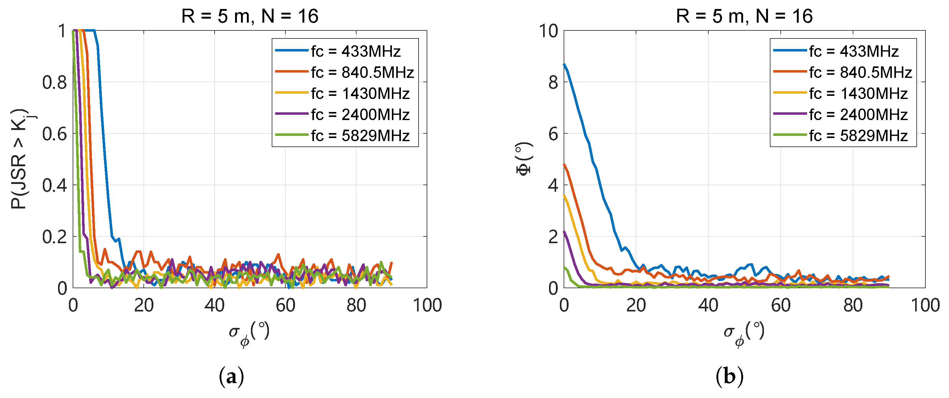
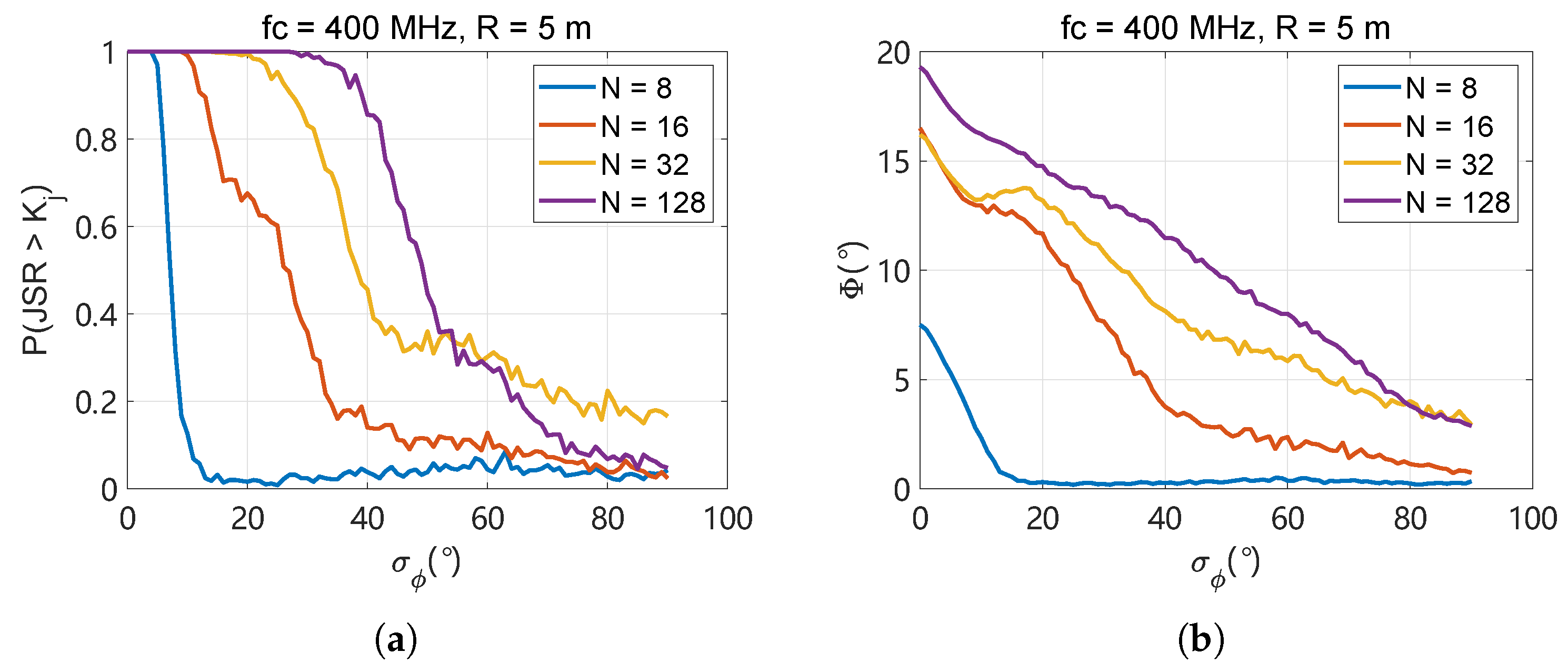
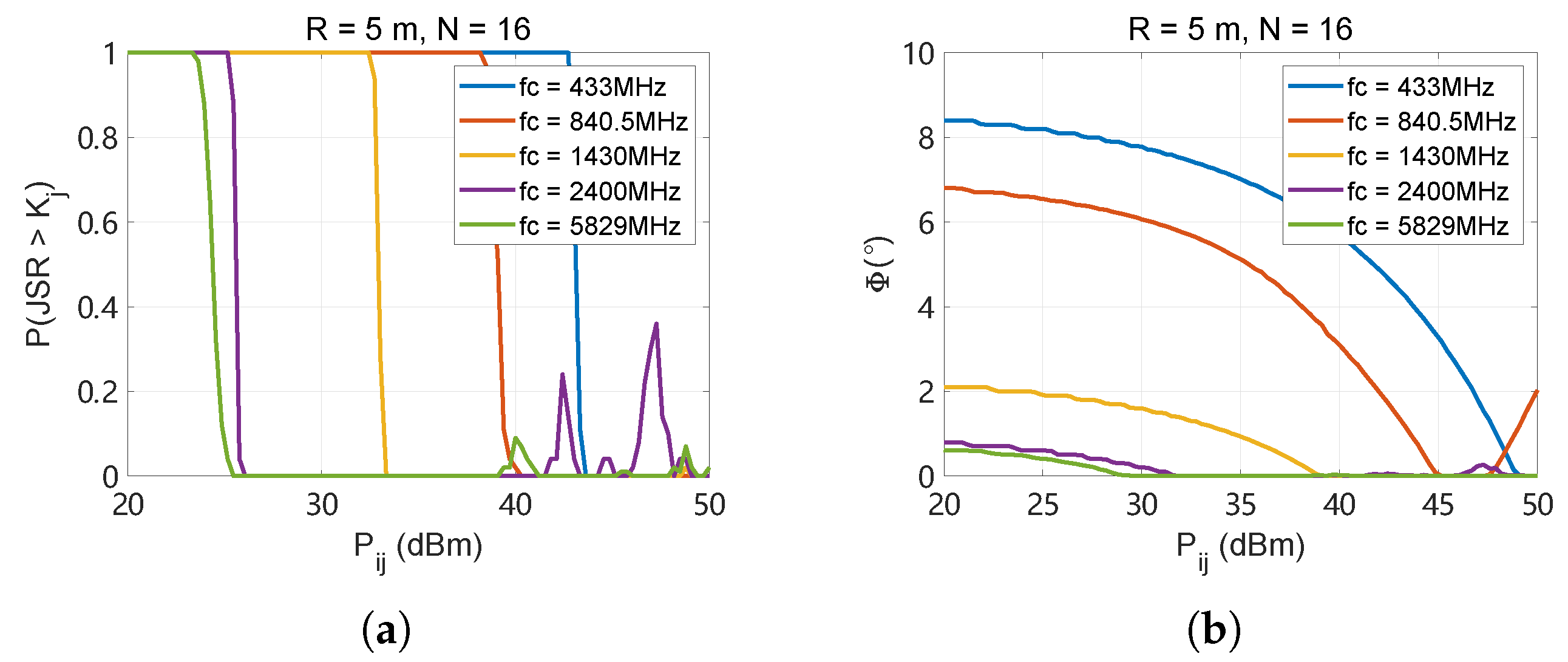
4.2.1. Jamming Performance with Azimuth Error

In order to analyze the jamming performance affected by $\mathrm{\Delta }{\varphi }_k$ and $\mathrm{\Delta }{r}_k$, respectively, firstly, increase the variance error (${\sigma }_{\varphi }$) of $\mathrm{\Delta }{\varphi }_k$ with $\mathrm{\Delta }{r}_k=0$, and ${\sigma }_{\varphi }$ conforms to Gaussian distribution. This paper mainly analyzes the positioning errors due to jitter and GPS (or other location technology), assuming that the time error $\mathrm{\Delta }{\tau }_k$ has been modified and that all nodes are synchronous. In addition, to obtain an accurate upper bound of the error based on the principle of control variables, $p_{ij}$ and $p_{is}$ are ignored when analyzing a single error. Furthermore, $p_{ij}$ and $p_{is}$ are at the same level in limited airspace, ${\widehat{P}}_{rs}$ and ${\widehat{P}}_{rj}$ are relatively stable, and setting $p_{ij}=p_{is}=0$ is feasible.

After several experiments under the same condition, the probability of $JS{R}_{av,0}$ being larger than $K_j$ ($P({\widehat{JSR}}_{av,0}>K_j)$) and ${\widehat{\mathrm{\Phi }}}_{av}$ is calculated. As shown in Figure 7a, with the increase in ${\sigma }_{\varphi }$, $P({\widehat{JSR}}_{av,0}>K_j)$ decreases totally, and the jamming performance at the high frequencies is worse than at the low frequencies. This occurs because the wavelength of the lower frequencies is longer than that of the high frequencies, the transmission loss is smaller, and the stability is higher. Since ${\sigma }_{\varphi }=0.6^{\circ }$, $P({\widehat{JSR}}_{av,0}>K_j)$ of the collaborative jamming array constructed with 16 nodes is already lower than 0.9. As the jamming frequency decreases to 433 MHz, the upper bound of ${\sigma }_{\varphi }$ is $7.5^{\circ }$ when $P({\widehat{JSR}}_{av,0}>K_j)\ge 0.9$.

Due to the increase in the error, the correlation of the jamming waveforms of each node decreases, which affects the jamming performance of the electromagnetic wave in the target area and results in a deviation in the beam direction from the target azimuth and a gradual reduction in ${\widehat{\mathrm{\Phi }}}_{av}$. Figure 7b shows the curve of ${\widehat{\mathrm{\Phi }}}_{av}$ with ${\sigma }_{\varphi }$. Since ${\sigma }_{\varphi }<{20}^{\circ }$, the low-frequency signal can cover more area than the high-frequency signal. This disparity can be attributed to the longer wavelengths associated with the lower frequencies, which allow for broader coverage. However, as ${\sigma }_{\varphi }$ continues to increase, ${\widehat{\mathrm{\Phi }}}_{av}$ correspondingly decreases, indicating a diminished capacity to maintain a wide jamming range under conditions of heightened azimuthal inaccuracies.

In order to further compare the influence of ${\sigma }_{\varphi }$ on jamming performance under different N, multiple experiments are carried out at the same frequency, and $P(\widehat{JSR}>K_j)$ is calculated in Figure 8a. The decline is steeper for smaller numbers of elements, indicating that systems with fewer elements are more sensitive to azimuthal errors while the larger arrays are more robust against azimuthal errors. This is because more nodes can converge stronger energy in the limited distribution space. Figure 8b depicts the effective jamming range as ${\sigma }_{\varphi }$ varies. Similar to $P(\widehat{JSR}>K_j)$, the effective range decreases with increasing ${\sigma }_{\varphi }$. However, the rate of decrease is less pronounced for larger arrays, indicating that larger arrays can maintain a broader jamming range even under higher azimuthal errors.

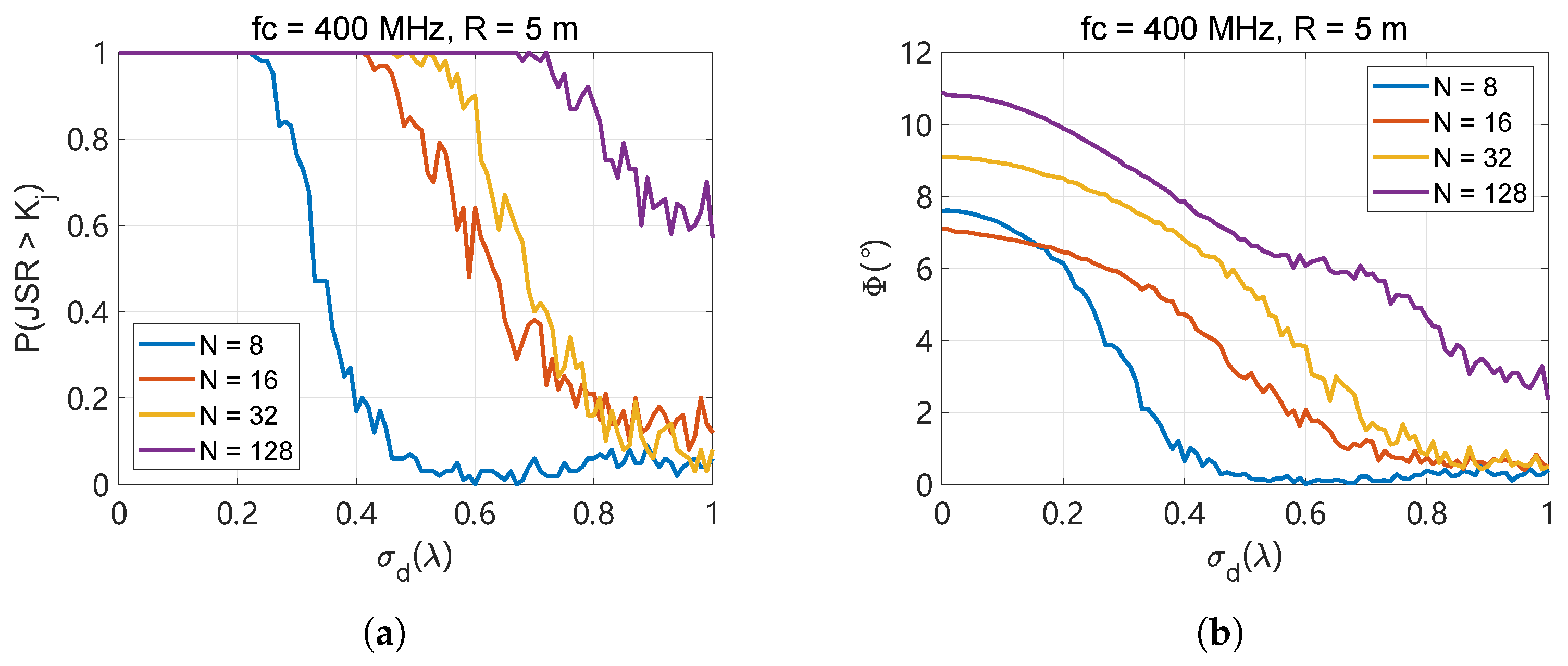
4.2.2. Jamming Performance with Distance Error

Distance error also affects the coherence of the waveforms, leading to a misalignment of the synthesized jamming beam with the target direction, ultimately reducing both $JS{R}_{av,0}$ and ${\mathrm{\Phi }}_{av}$. The upper bounds of $P({\widehat{JSR}}_{av,0}>K_j)=0.9$ are calculated based on different variances of ${\sigma }_d$, which ranges from 0 to $\lambda$.

Figure 9a illustrates the impact of distance error ${\sigma }_d$ on the probability of successful jamming $P({\widehat{JSR}}_{av,0}>K_j)$ across different frequencies. As ${\sigma }_d$ increases, $P({\widehat{JSR}}_{av,0}>K_j)$ gradually decreases. Notably, lower-frequency signals exhibit a heightened resilience against such errors. This phenomenon arises from the longer wavelength of low-frequency signals, which mitigates phase misalignment caused by distance errors, thereby maintaining higher JSR stability. In contrast, high-frequency signals with shorter wavelengths are more sensitive to phase errors, leading to a rapid decline in jamming effectiveness as ${\sigma }_d$ increases. Complementing this, Figure 9b illustrates the effective jamming range ${\widehat{\mathrm{\Phi }}}_{av}$ versus ${\sigma }_d$. For a given ${\sigma }_d$, the lower-frequency signals can cover a larger jamming range compared to their higher-frequency counterparts. This behavior is attributed to the broader beamwidth of low-frequency signals, which ensures wider coverage despite phase misalignment.

At a frequency of 400 MHz, $P({\widehat{JSR}}_{av,0}>K_j)$ is calculated, which is shown in Figure 10a. As ${\sigma }_d$ increases, $P({\widehat{JSR}}_{av,0}>K_j)$ gradually decreases. With fewer nodes, $P({\widehat{JSR}}_{av,0}>K_j)$ decreases more rapidly to below 0.9. This trend is attributed to the enhanced phase coherence and redundancy provided by a higher number of nodes, which mitigate the impact of distance errors on beamforming performance. Consequently, increasing N within resource constraints significantly improves the array’s stability, ensuring a higher probability of effective jamming even under moderate distance errors. And, with fewer nodes, ${\widehat{\mathrm{\Phi }}}_{av}$ also reduces faster, which is illustrated in Figure 10b. This behavior is due to the reduced spatial diversity and phase coherence in smaller arrays, which amplify the detrimental effects of distance errors on beamforming. In contrast, larger arrays maintain a more stable ${\widehat{\mathrm{\Phi }}}_{av}$ even at higher ${\sigma }_d$, owing to their improved ability to compensate for phase misalignment. These results emphasize the importance of node density in maintaining robust jamming performance and preserving the effective jamming range in distributed systems.

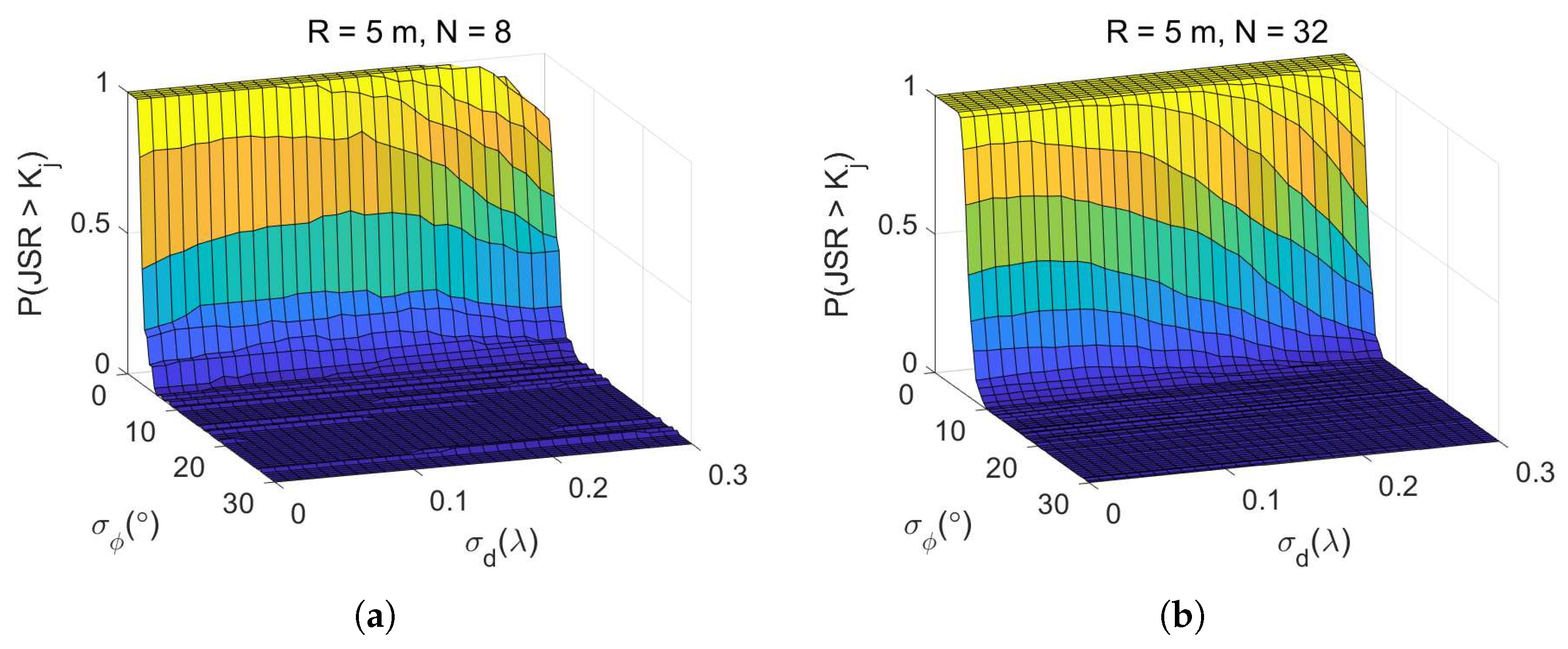
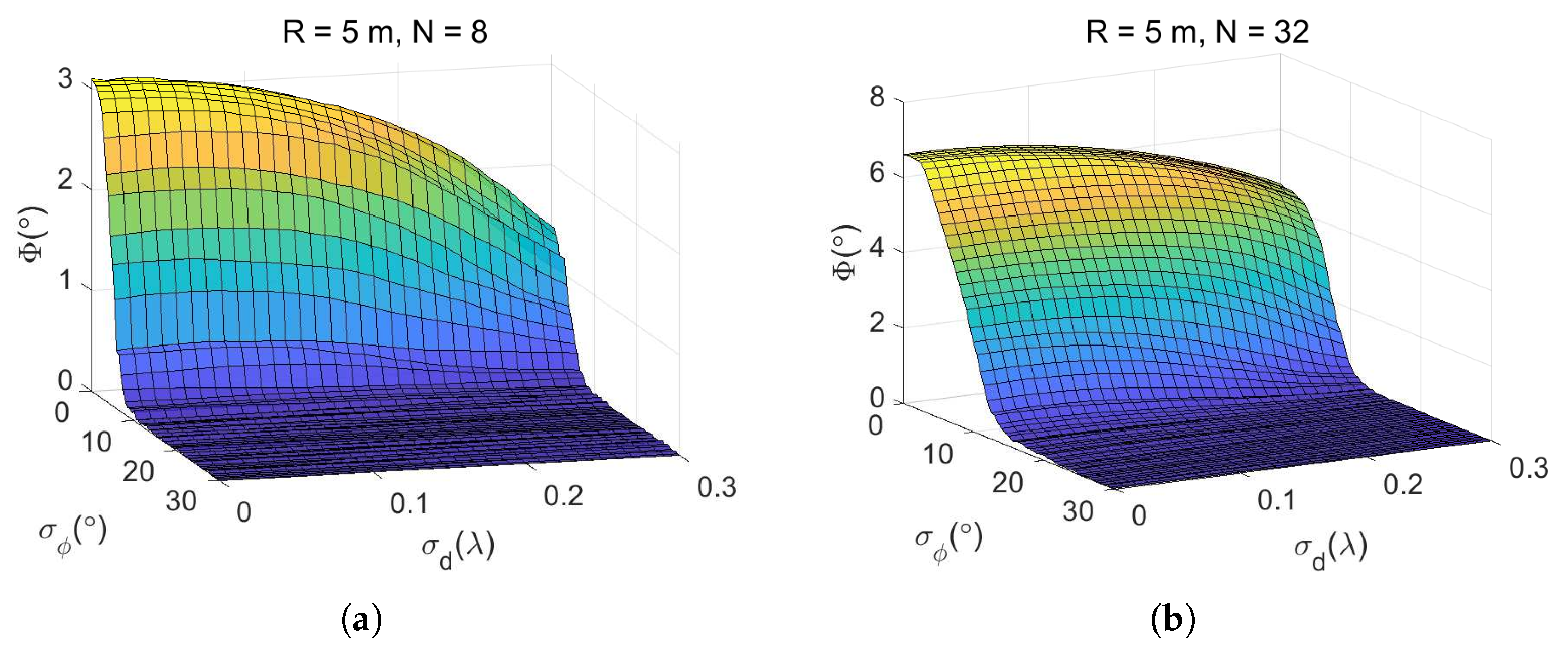
4.2.3. Joint Analysis of Positioning Errors

The azimuth and distance errors will act on the distributed nodes simultaneously, affecting the formation of the jamming beam. In the case of ${\sigma }_{\varphi }<{30}^{\circ },{\sigma }_d<0.3$, multiple experiments are carried out to calculate the upper bounds.

When N is 8 and 32, the joint results of positioning errors are compared. As shown in Figure 11, the impact of ${\sigma }_{\varphi }$ on $P({\widehat{JSR}}_{av,0}>K_j)$ is more significant. When ${\sigma }_d$ remains unchanged, ${\sigma }_{\varphi }$ increases to $5^{\circ }$ and $P({\widehat{JSR}}_{av,0}>K_j)$ will drop sharply. Finally, when ${\sigma }_{\varphi }=7^{\circ }$, $P({\widehat{JSR}}_{av,0}>K_j)$ is close to 0, and the jamming is completely ineffective. This indicates that the azimuth error has a more direct influence on beam direction and phase coherence, which are critical for effective jamming. In contrast, while ${\sigma }_{\varphi }$ is well controlled, ${\sigma }_d$ has a relatively minor impact on jamming effectiveness. After N increases to 32, the stability of the array is improved when ${\sigma }_{\varphi }<6^{\circ },{\sigma }_d<0.2$, $P({\widehat{JSR}}_{av,0}>K_j)$ can be maintained at 1, demonstrating the robustness of larger arrays against positioning errors. However, when ${\sigma }_d$ increases to 0.25, $P({\widehat{JSR}}_{av,0}>K_j)$ shows a downward trend, indicating that, even with a higher node count, excessive distance errors can degrade performance. In order to control $P({\widehat{JSR}}_{av,0}>K_j)\ge 0.9$, it is necessary to ensure that ${\sigma }_{\varphi }<5^{\circ },{\sigma }_d<0.2$.

In terms of ${\widehat{\mathrm{\Phi }}}_{av}$, the results are shown in Figure 12. The impact of ${\sigma }_{\varphi }$ is significantly greater than that of ${\sigma }_d$. When ${\sigma }_{\varphi }>{10}^{\circ }$, effective jamming can no longer be achieved in the target area. This underscores the critical necessity of maintaining ${\sigma }_{\varphi }$ within a tighter tolerance. When $N=32$, ${\widehat{\mathrm{\Phi }}}_{av}$ can be maintained above $8^{\circ }$ to some extent as positioning errors increase, showing improved stability against errors. This improvement is attributed to the larger number of nodes, which contributes to a more robust jamming pattern capable of withstanding higher error rates. The decrease in effective range slows down compared to $N=8$, indicating that a denser node deployment can effectively mitigate the adverse effects of positioning inaccuracies. However, this resilience is not without limits. Until ${\sigma }_{\varphi }>{20}^{\circ }$ and ${\sigma }_d>0.3\lambda$, the benefits of coordinated jamming are nullified, leading to a complete loss of jamming effectiveness. This threshold highlights the practical constraints within which jamming systems may operate effectively.

To investigate the inter-relationship between the azimuth error and the distance error, different lower bounds for $P({\widehat{JSR}}_{av,0}>K_j)$ are set. This led to the derivation of the upper bound variation curve for the azimuth error under different distance errors, as shown in Figure 13. As ${\sigma }_d$ increases, the upper bound of ${\sigma }_{\varphi }$ decreases. This trend is consistent across all subplots and all probability bounds, suggesting that more precise azimuth estimations can compensate for larger distance errors and vice versa. As the lower bound of $P({\widehat{JSR}}_{av,0}>K_j)$ increases, the precision requirements for both the azimuth and the distance errors also increase. This is evident from the steeper slopes of the curves in each subplot as the probability bound increases from 0.5 to 0.9. The curves demonstrate that higher success probabilities necessitate tighter control over positioning errors to achieve effective jamming. The augmentation of the number of nodes N is directly correlated with a diminished upper boundary for both ${\sigma }_{\varphi }$ and ${\sigma }_d$. This trend is uniformly observable across all subplots, indicating that larger arrays exhibit enhanced error resilience. The reduction in error bounds with increasing N suggests that larger arrays can more efficaciously mitigate the impact of positioning inaccuracies, culminating in a more robust jamming performance. The capability to select pertinent curves based on the jamming array’s node count facilitates the optimization of positioning methodologies. This adaptability ensures that the jamming system can be configured to align with particular operational criteria while preserving cost-effectiveness. The analysis offers invaluable insights into how diverse array configurations influence error tolerance, which is essential for deploying effective coordinated electronic countermeasures.

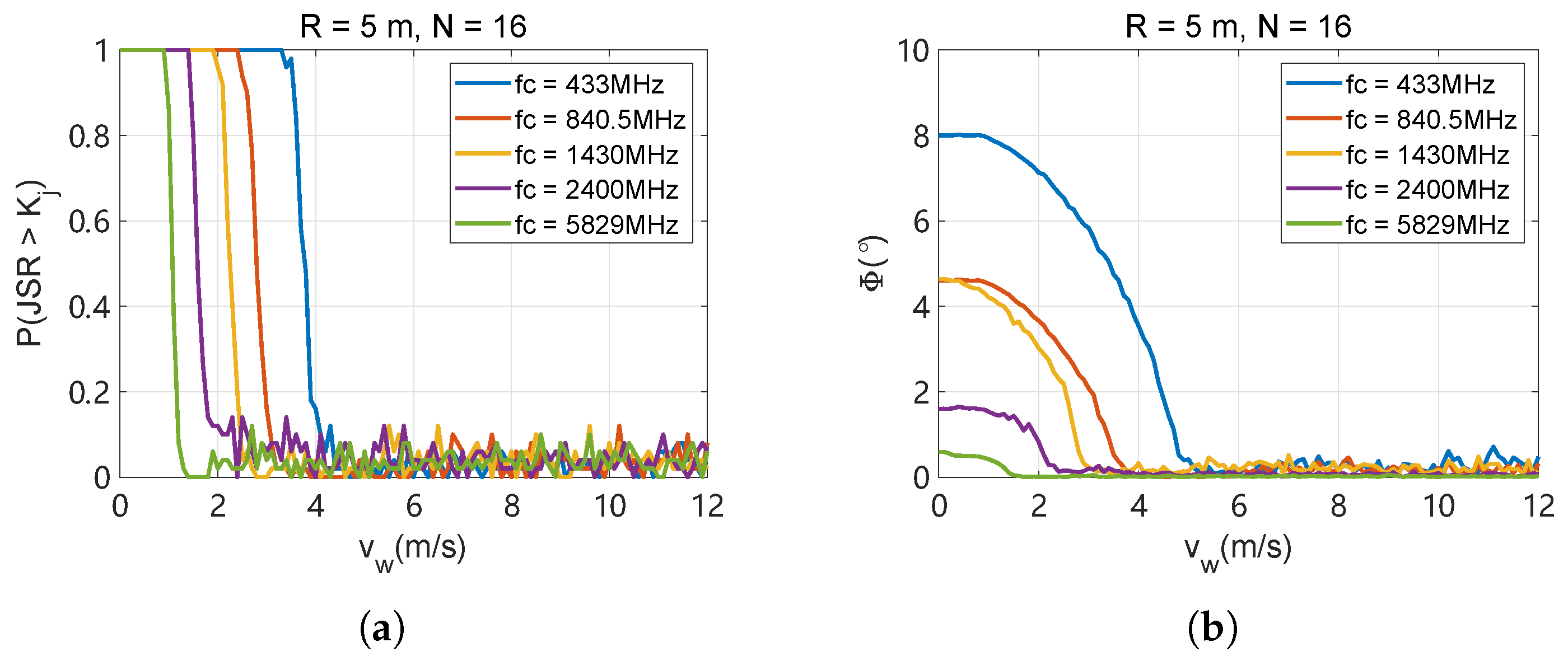
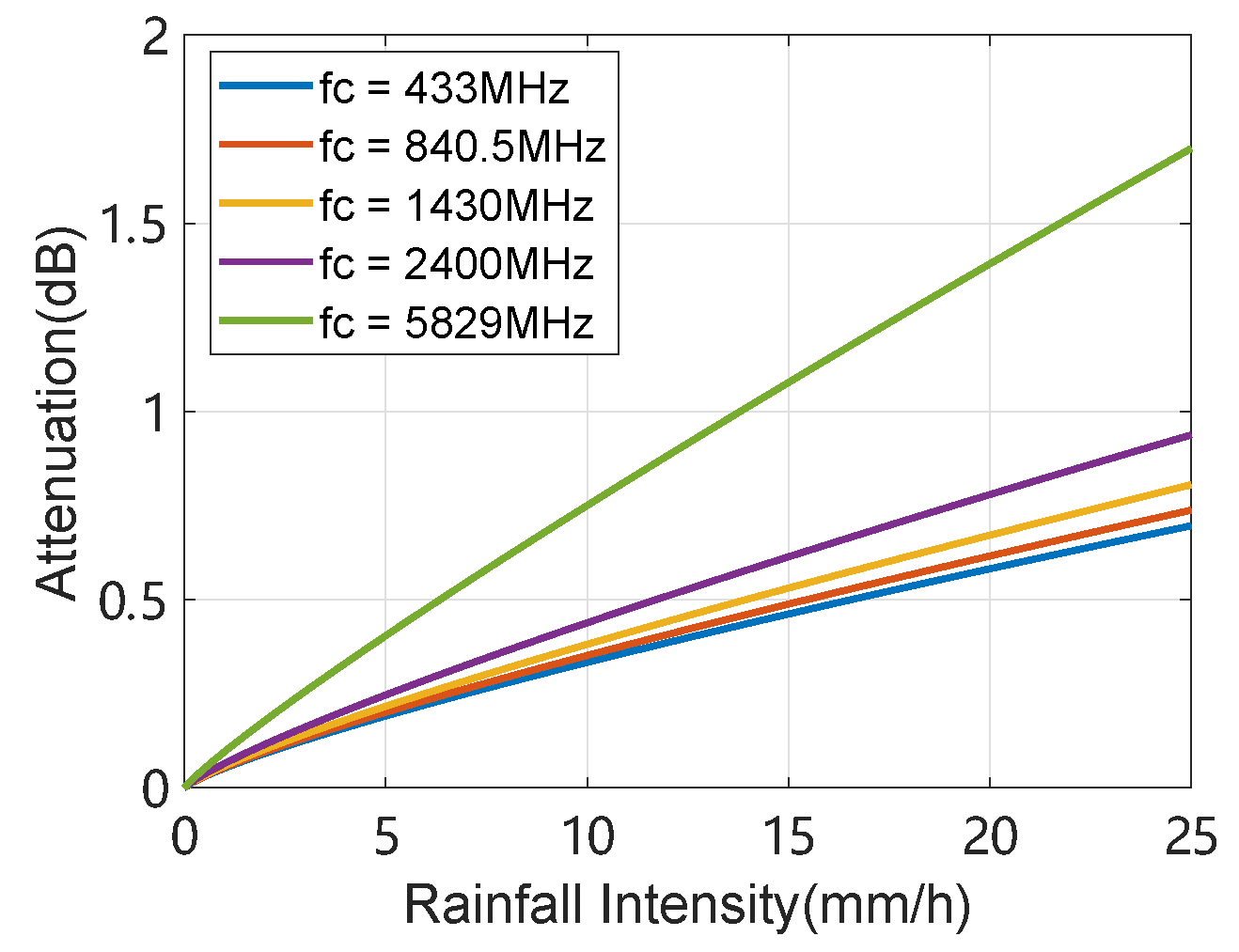
4.2.4. Jamming Performance in Different Environments

To comprehensively analyze the impact of various real-world factors on jamming effects, this section evaluates the influence of wind speed, precipitation, and other external interference sources on UAV attitude and GPS signal performance. The following analysis aims to better understand how these environmental and external factors contribute to the overall interference landscape.

(1)

Wind speed

Assume that the aerial wind speed is $v_w$; the yaw dynamics equation is given by the following [38]:

$$b_{\psi }\mathrm{\Delta }\varphi ={\tau }_y$$

(32)

where $b_{\psi }$ represents the yaw damping coefficient and $\mathrm{\Delta }\varphi$ denotes the azimuth angle deviation. The wind-induced torque ${\tau }_y$ caused by the wind speed $v_w$ is expressed as

$${\tau }_y={\displaystyle \frac{1}{2}}{\rho }_a{C}_{lat}Al{v}_w^2$$

(33)

where ${\rho }_a$ is the air density, $C_{lat}$ is the lateral force coefficient, A is the frontal area, and l is the moment arm length. By combining Equations (32) and (33), the azimuth angle deviation can be derived as

$$\mathrm{\Delta }\varphi ={\displaystyle \frac{{\tau }_y}{b_{\psi }}}={\displaystyle \frac{{\rho }_a{C}_{lat}Al{v}_w^2}{2b_{\psi }}}$$

(34)

During UAV hover, the thrust T and wind force $F_w$ should satisfy the following equilibrium condition:

$$T=\sqrt{{\left(mg\right)}^2+F_w^2}$$

(35)

where $mg$ represents the gravitational force of the UAV. The wind force is expressed as follows [39,40]:

$$F_w={\displaystyle \frac{1}{2}}{\rho }_a{C}_{d}A{v}_w^2$$

(36)

where $C_d$ is the drag coefficient. When $T\ge T_{max}$ (the maximum thrust of the UAV), hover fails. The critical wind speed is given by

$$v_{\mathrm{crit}}=\sqrt{{\displaystyle \frac{2(T_{max}-mg)}{{\rho }_a{C}_{d}A}}}$$

(37)

For $v_w\le v_{crit}$, the displacement $\mathrm{\Delta }r$ is expressed as

$$\mathrm{\Delta }r={\displaystyle \frac{F_w}{k_{\mathrm{spring}}}}$$

(38)

where $k_{\mathrm{spring}}$ is the equivalent spring stiffness, representing the wind resistance capability of the UAV’s flight control system.

For $v_w>v_{crit}$, the UAV accelerates under the wind force, and the equation of motion is

$$ma=F_w-F_{\mathrm{drag}}$$

(39)

where a is the acceleration, $F_{\mathrm{drag}}={\displaystyle \frac{1}{2}}{\rho }_a{C}_{d}A{v}^2$ is the aerodynamic drag during UAV movement, and v is the moving speed. When $a=0$, the steady-state speed is solved as

$$v_{\mathrm{steady}}=\sqrt{{\displaystyle \frac{2(F_w-mg)}{{\rho }_a{C}_{d}A}}}=\sqrt{v_w^2-v_{\mathrm{crit}}^2}$$

(40)

Integrating yields the following displacement:

$$\mathrm{\Delta }r(t)={\displaystyle \frac{m}{{\rho }_a{C}_{d}A}}ln\left(cosh\left(\sqrt{{\displaystyle \frac{{\rho }_a{C}_{d}A}{m}}}·t·v_{\mathrm{steady}}\right)\right)$$

(41)

For short durations ($t\ll \sqrt{m/\left({\rho }_a{C}_{d}A{v}_{\mathrm{steady}}\right)}$), $\mathrm{\Delta }d\left(t\right)$ is approximated as

$$\mathrm{\Delta }d(t)\approx {\displaystyle \frac{1}{2}}\left(v_w^2-v_{\mathrm{crit}}^2\right)t^2$$

(42)

Taking the DJI M300 as an example, with a maximum tolerable wind speed of 12 m/s, the horizontal jitter and displacement of each UAV were calculated under different wind speed levels. Multiple experiments were conducted for different carrier frequencies, and the jamming performance is shown in Figure 14. Figure 14a illustrates the variation in $P(JSR>K_j)$ with wind speed at different frequencies. It is evident that, as the wind speed increases, the UAV jitter becomes more pronounced, and the beams emitted by each node become more unstable. Due to their shorter wavelengths, higher frequencies are more severely affected than lower frequencies under the same jamming conditions. Figure 14b demonstrates the impact of wind speed on the effective jamming range. As the wind force increases, the uncertainty in the beam phase also rises, preventing optimal beam interference and reducing the high-power coverage area. High-frequency signals are more sensitive to jitter, resulting in narrower beam widths under the same wind speed conditions as low-frequency signals.

(2)

Rainfall intensity

The attenuation of electromagnetic wave propagation due to rainfall is also critical in wireless communication systems, particularly at higher frequencies. The specific attenuation $A_{rain}$ caused by rainfall can be modeled as a function of the carrier frequency $f_c$, rainfall intensity I, and propagation distance $d_k$. The relationship is expressed as follows [41]:

$$A_{\mathrm{rain}}=a\left(f\right)·I^{b\left(f\right)}·d_k$$

(43)

where $a\left(f\right)$ and $b\left(f\right)$ are frequency-dependent coefficients that characterize the attenuation properties of rainfall. The coefficients $a\left(f\right)$ and $b\left(f\right)$ are typically derived from empirical data and can be expressed as polynomial functions of frequency:

$$\begin{array}{cc}\hfill a\left(f\right)& =a_0+a_{1}f+a_2{f}^2\hfill \\ \hfill b\left(f\right)& =b_0+b_{1}f+b_2{f}^2\hfill \end{array}$$

(44)

Here, $a_0,a_1,a_2,b_0,b_1$, and $b_2$ are fitting parameters that depend on the specific frequency band and environmental conditions.

Based on the attenuation model, the extent of attenuation under different rainfall intensities has been determined. The DJI M300, with an IP45 protection rating, can withstand a maximum rainfall intensity of 25 mm/h. As shown in Figure 15, the loss during electromagnetic wave transmission increases as the rainfall intensity increases. Higher frequencies experience more substantial attenuation under the same rainfall intensity. The maximum attenuation observed is 1.7 dB within the results, which is almost negligible compared to the path loss.

(3)

External source of interference

Weather conditions, such as strong winds and rainfall, can significantly affect the stability of a drone’s attitude. In real-world scenarios, various sources of electromagnetic interference can further degrade the signal-to-interference-plus-noise ratio (SINR) of GPS signals, thereby introducing positioning errors. To quantify the impact of interference on GPS positioning performance, it is necessary to theoretically analyze the sources of range errors and azimuth errors and their relationship with the SINR.

The SINR is a key metric for evaluating signal quality and is given by

$$\mathrm{SINR}={\displaystyle \frac{P_r}{P_n+P_i}}$$

(45)

where $P_r$ is the received signal power of the GPS, $P_n$ is the noise power, and $P_i$ is the interference power. Pseudorange measurement errors primarily cause the range error $\mathrm{\Delta }r$, and its magnitude is inversely proportional to the square root of $\mathrm{SINR}$. The range error can be expressed as

$$\mathrm{\Delta }r={\displaystyle \frac{K_{\rho }}{\sqrt{\mathrm{SINR}}}}$$

(46)

where $K_{\rho }$ is the range error proportionality constant, which depends on the receiver’s performance and signal propagation environment.

The azimuth error is determined by both the range error and the satellite geometry, represented by the horizontal dilution of precision (HDOP). The azimuth error can be derived as

$$\mathrm{\Delta }\varphi =\mathrm{\Delta }\rho \times \mathrm{HDOP}$$

(47)

HDOP is a dimensionless value that reflects the impact of satellite geometry on horizontal positioning accuracy. A higher HDOP value indicates a greater amplification effect of positioning errors due to range errors.

This section analyzes the impact of varying levels of external interference on GPS L1 signals. The results, as shown in Figure 16a, demonstrate that, as the power of external interference increases, the SINR of the GPS signal decreases. This degradation in SINR directly impairs the ability of the drone’s positioning module to resolve accurate location information, thereby affecting the energy efficiency of the jamming beam. In Figure 16b, the effective jamming range is shown to shrink as external interference increases. This phenomenon occurs because the beamforming nodes, influenced by positioning errors, fail to align accurately with the target, resulting in a more dispersed beam pattern. Consequently, the concentration of energy in the intended direction diminishes, reducing the overall performance of the jamming.

5. Comprehensive Experiment

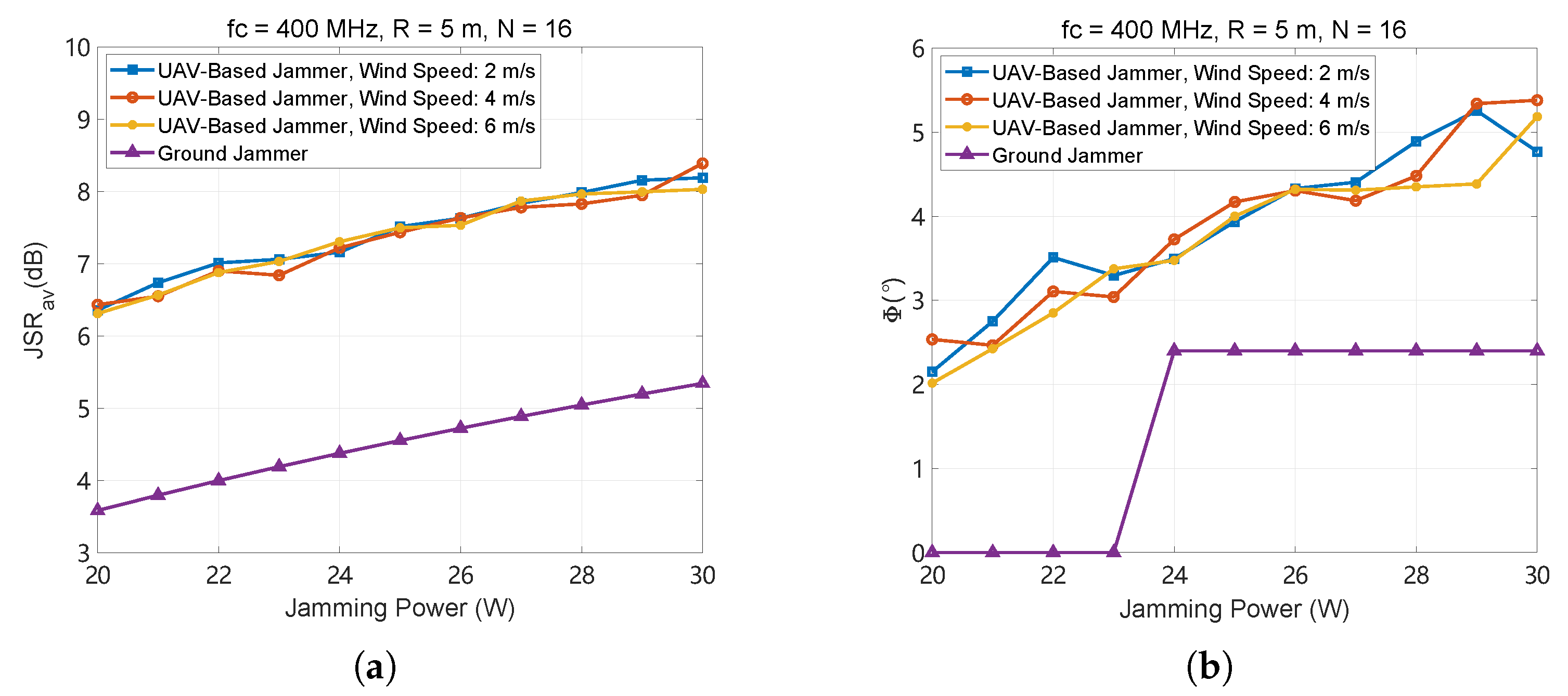
5.1. Simulation-Based Jamming Analysis in Realistic Scenarios

To verify the practical applicability of the upper bound of the azimuth and the distance error, a comprehensive experiment is carried out. The wind and the GPS instability cause both the azimuth and the distance error. Assume that the wind speed is 6 m/s and that the rainfall intensity is 10 mm/h. The external source of interference is also considered in the experiment. The environment noise $P_n$ and the external interference $P_i$ are set to −110 dBm and 45 dBm, respectively. The transmitted power of the jamming node is set to 1 dBm, while $P_{ts}$ is also set to 1 dBm. In addition, the distance between the jamming array and the target is 1 km, and the base station is 200 m away from the target.

The experimental outcomes depicted in Figure 17 provide a detailed examination of the impact of the azimuth error ${\sigma }_{\varphi }$ and the distance error ${\sigma }_d$ on ${\widehat{JSR}}_{av,0}$. As ${\sigma }_{\varphi }$ varies from $1^{\circ }$ to $5^{\circ }$ and ${\sigma }_d$ varies from $0.22\lambda$ to $0.35\lambda$, the plots reveal a consistent trend of decreasing ${\widehat{JSR}}_{av,0}$ with increasing positioning errors. This reduction signifies a degradation in the effectiveness of the jamming signal as the errors perturb the phase of the individual waves, thereby disrupting the coherence necessary for optimal beam steering. The plots illustrate that as ${\sigma }_{\varphi }$ increases, the peak of the ${\widehat{JSR}}_{av,0}$ curve, which represents the maximum jamming effectiveness, shifts away from the target direction ${\varphi }_0$. This shift indicates the beam’s main lobe deviating from the intended direction, leading to a less focused jamming pattern. Additionally, the amplitude of the ${\widehat{JSR}}_{av,0}$ diminishes with greater ${\sigma }_{\varphi }$, suggesting that not only is the beam misaligned but its overall effectiveness is also reduced. Similar to the azimuth error, an increase in ${\sigma }_d$ also decreases the ${\widehat{JSR}}_{av,0}$ peak values and a broadening of the main lobe. This broadening effect reduces the beam’s directivity, making it less effective at targeting specific directions. The distance error contributes to a more dispersed jamming pattern, as the phase discrepancies among the waves from different array elements become more pronounced, further diminishing the beam’s ability to concentrate energy toward ${\varphi }_0$. The yellow line at $K_j=6\mathrm{dB}$ acts as a threshold indicating the minimum required ${\widehat{JSR}}_{av,0}$ for successful jamming. As both ${\sigma }_{\varphi }$ and ${\sigma }_d$ increase, the ${\widehat{JSR}}_{av,0}$ curves approach and eventually fall below this threshold, signaling a failure to maintain effective jamming.

After a series of experiments, the jamming success probability $P({\widehat{JSR}}_{av,0}>K_j)$ and the effective jamming range ${\widehat{\mathrm{\Phi }}}_{av}$ with different positioning errors are analyzed. As shown in

Table 1. The jamming success probability $P(JS{R}_{av,0}>K_j)$ and the effective jamming range ${\widehat{\mathrm{\Phi }}}_{av}$ with different positioning errors.

Parameters	Data				Unit
${\sigma }_{\varphi }$	1	3.1	4.2	5	${}^{\circ }$
${\sigma }_d$	0.22	0.25	0.28	0.35	$\lambda$
$P({\widehat{JSR}}_{av,0}>K_j)$	100%	87%	58%	34%	/
${\widehat{\mathrm{\Phi }}}_{av}$	4.9	4.5	4.0	2.9	${}^{\circ }$

, the comprehensive analysis of both ${\sigma }_{\varphi }$ and ${\sigma }_d$ reveal their synergistic impact on the effectiveness of jamming operations. As ${\sigma }_{\varphi }$ escalates from $1^{\circ }$ to $5^{\circ }$ and ${\sigma }_d$ escalates from $0.22\lambda$ to $0.35\lambda$, there is a marked reduction in the jamming success probability, plummeting from 100% to 34%, and a concurrent contraction of the effective jamming range from $4.9^{\circ }$ to $2.9^{\circ }$. This decline is attributed to the errors’ propensity to misalign the jamming beam from the target direction, thereby undermining the jamming efficiency. The interplay between these errors underscores the imperative for meticulous positioning accuracy to sustain optimal jamming performance, highlighting that even modest increases in positioning discrepancies can significantly curtail the operational scope and success rate of jamming endeavors.

In conclusion, the experimental results underscore the critical role of precise positioning in maintaining the effectiveness of jamming signals. As both the azimuth and distance error increase, the jamming signal’s ability to target and maintain jamming over a desired area significantly diminishes, highlighting the need for robust error mitigation strategies in practical applications.

5.2. Comparison with Ground-Based Systems

The collaborative and mobile nature of unmanned aerial vehicles (UAVs) enables them to perform jamming operations at closer proximity to the target. The air-to-ground transmission channel, characterized by a higher probability of line-of-sight (LoS) propagation, significantly mitigates the losses caused by multipath effects. This presents a notable advantage over ground-based jamming devices, which are often hindered by severe multipath fading and shadowing in terrestrial environments. In this section, we conduct experimental comparisons to validate this advantage and demonstrate the superior effectiveness of UAV-assisted jamming in terms of interference–signal ratio (JSR) performance.

In a multipath environment, the received jamming power is the sum of the powers from all paths, including the direct path and reflected/scattered paths. The total received jamming power $P_{rj}^G$ is

$$P_{rj}^G=\sum _{n=1}^N{P}_{j,n}+\sum _{n\ne m}{\alpha }_n{\alpha }_m^{\ast }{R}_s({\tau }_n-{\tau }_m)\sqrt{P_{j,n}{P}_{j,m}}$$

(48)

where $P_{j,n}$ is the received power from the n-th path, ${\alpha }_n$ is the complex gain of the n-th path, $R_s({\tau }_n-{\tau }_m)$ is the autocorrelation function of the signal, representing the correlation between the n-th and m-th paths, and ${\tau }_n$ and ${\tau }_m$ are the delays of the n-th and m-th paths, respectively.

Therefore, the JSR of the ground jammer is given by

$$JS{R}_G={\displaystyle \frac{P_{rj}^G}{P_{rs}}}$$

(49)

In this experiment, the impact of ground-based jamming equipment on a target receiver in a multipath environment is investigated, focusing on the relationship between jamming power, jamming effectiveness, and effective jamming range under varying wind conditions. The setup consists of 16 UAVs distributed within a 5 m radius at a distance of 1 km from the target, each transmitting within a total power range of 20–30 W, and the variance in azimuth error and distance error is $1^{\circ }$ and $0.22\lambda$, respectively. Moreover, a ground-based jammer is located 2.5 km from the target with a jamming beamwidth of 20 degrees and a power range of 20–30 W. The carrier frequency is set to 400 MHz, with environmental noise and external interference levels of −110 dBm and 45 dBm, respectively. Under different wind speeds, the relationship curves of jamming power with jamming effect and effective jamming range are obtained.

The results depicted in Figure 18a illustrate the relationship between the $JS{R}_{av}$ and the jamming power for both UAV-based jammers and a ground-based jammer under different wind speeds. As the jamming power increases from 20 W to 30 W, the JSR for all configurations shows a corresponding increase, indicating improved jamming effectiveness with higher power levels. However, the ground-based jammer consistently exhibits lower JSR values than the UAV-based jammers. This discrepancy is primarily attributed to multipath fading, which causes the energy transmitted by the ground-based jammer to disperse and not effectively concentrate on the target area, thereby reducing its jamming efficiency. The impact of the wind speed on the UAV-based jammers is minimal, as they can stabilize their position in the air despite wind speeds of 2 m/s, 4 m/s, and 6 m/s. This stability allows the UAV-based jammers to maintain precise targeting and effective energy concentration on the target, showcasing a significant advantage over the ground-based jammer. Similarly, Figure 18b depicts the variation in the effective jamming range $\mathrm{\Phi }$ concerning jamming power for both UAV-based and ground-based jammers under different wind speeds. As the jamming power increases, $\mathrm{\Phi }$ grows, reflecting a broader jamming coverage at higher power levels. However, the ground-based jammer consistently achieves a smaller effective jamming range than the UAV-based jammers. Furthermore, due to the distributed characteristics of the UAV array, the UAV-based jammers exhibit a significantly more extensive effective jamming range. At different wind speeds, the stability of the UAV array is also demonstrated.

6. Conclusions

In collaborative jamming, when multiple waveforms meet the requirements of being coherent, they can achieve jamming in the target area, resulting in a quadratic increase in jamming power. The contrast experiment demonstrates that this approach offers superior jamming effectiveness and flexibility compared to ground-based jammers. Precise positioning and a synchronized launching time are necessary conditions for phase synchronization. When there are distance and azimuth errors, this directly leads to deviations in beam direction and power loss. Using UAVs as jamming nodes, various complex factors during flight can introduce positioning errors. This paper analyzes the upper bound of the azimuth and distance error required to achieve effective jamming under different frequencies, distribution radii, and node counts. The upper bounds of ${\sigma }_{\varphi }$ and ${\sigma }_d$ corresponding to $P(\widehat{JSR}>K_j)\ge 0.9$ are summarized in

Table 2. The requirements of ${\sigma }_{\varphi }$ and ${\sigma }_d$ versus carrier frequency $f_c$ when $P(\widehat{JSR}>K_j)\ge 0.9$. The distributed range R is 5 m and the number of nodes N is 16.

Parameters	Data					Unit
$f_c$	433	840.5	1430	2400	5829	MHz
${\sigma }_{\varphi }$	7.2	4.09	2.55	1.34	0.28	${}^{\circ }$
${\sigma }_d$	0.29	0.15	0.09	0.05	0.02	m

and

Table 3. The requirements of ${\sigma }_{\varphi }$ and ${\sigma }_d$ versus the number of nodes N when $P(\widehat{JSR}>K_j)\ge 0.9$. The carrier frequency $f_c$ is 400 MHz and the distributed range R is 5 m.

Parameters	Data				Unit
N	8	16	32	128	/
${\sigma }_{\varphi }$	5.35	12.65	27.44	39.05	${}^{\circ }$
${\sigma }_d$	0.20	0.35	0.43	0.57	m

.

Additionally, the comprehensive experiments bring the error analysis closer to real-world scenarios, providing reliable guidance for the rational deployment of nodes and the selection of positioning methods in practical electronic countermeasures. However, conducting experiments in real-world environments poses significant challenges due to uncontrollable factors, such as UAV jitter, electromagnetic interference, and GPS signal inaccuracies, making it difficult to measure true errors accurately. A potential solution is to experiment in a controlled environment, such as an anechoic chamber, where electromagnetic interference is minimized. Precision-controlled inertial navigation systems and gyroscopes can be used to measure positioning errors, while a receiver equipped with a rotating platform can assess jamming power and the effective jamming range. In future work, gyroscopes and positioning modules with varying performance levels will be mounted on UAVs to evaluate the impact of positioning errors on jamming effectiveness, particularly in GPS-denied environments, where inertial navigation systems are essential for estimating UAV position and velocity. A software-defined radio-based receiver will be employed to calculate jamming power under different error conditions and provide feedback on the effective jamming range. This approach will enhance the practical applicability of the study and address real-world implementation challenges.

References

1. Moseley, R.H. A Neural Network Classifier for Fault Correlation and Root Cause Determination in an Electronic Warfare System. In Proceedings of the AIAA SciTech Forum and Exposition, San Diego, CA, USA, 7–11 January 2019. [Google Scholar]
2. Jung, S. A Study on the Application of Artificial Intelligence for Naval Electronic Warfare. J. KNST 2020, 3, 118–124. [Google Scholar] [CrossRef]
3. Li, X.; Zhao, X.; Pu, W. An approach for predicting digital material consumption in electronic warfare. Def. Technol. 2020, 16, 263–273. [Google Scholar] [CrossRef]
4. Rahman, A.D.B.A.; Ghani, K.A.; Khamis, N.H.H.; Sidek, A.R.M. Unmanned Aerial Vehicle (UAV) GPS Jamming Test by using Software Defined Radio (SDR) platform. J. Phys. Conf. Ser. 2021, 1793, 012060. [Google Scholar]
5. Gao, Y.; Lv, N. UAV Swarm Cooperative Situation Awareness Theory Model Construction and Scenario Analysis. J. Phys. Conf. Ser. 2023, 2504, 012013. [Google Scholar]
6. Zhou, Y.; Rao, B.; Wang, W. UAV Swarm Intelligence: Recent Advances and Future Trends. IEEE Access 2020, 8, 183856–183878. [Google Scholar] [CrossRef]
7. Long, X.X.; Gao, F. Cooperative attack based on small-unit UAV swarms formation with trajectory tracking. J. Intell. Fuzzy Syst. 2023, 45, 2949–2965. [Google Scholar]
8. Javed, S.; Hassan, A.; Ahmad, R.; Ahmed, W.; Ahmed, R.; Saadat, A.; Guizani, M. State-of-the-Art and Future Research Challenges in UAV Swarms. IEEE Internet Things J. 2024, 11, 19023–19045. [Google Scholar] [CrossRef]
9. Xu, X.; Yan, X.; Yang, W.; An, K.; Huang, W.; Wang, Y. Algorithms and applications of intelligent swarm cooperative control: A comprehensive survey. Prog. Aerosp. Sci. 2022, 135, 100869. [Google Scholar] [CrossRef]
10. Abdelkader, M.; Guler, S.; Jaleel, H.; Shamma, J. Aerial Swarms: Recent Applications and Challenges. Curr. Robot. Rep. 2021, 2, 309–320. [Google Scholar] [CrossRef]
11. Paulsen, L.; Hoffmann, T.; Fulton, C.; Yeary, M.; Murmann, B. Impact: A low cost, reconfigurable, digital beamforming common module building block for next generation phased arrays. In Proceedings of the Open Architecture/Open Business Model Net-Centric Systems and Defense Transformation 2015, Tysons Corner, VA, USA, 13–16 April 2015. [Google Scholar]
12. Zhang, Y.; Cheng, R. Joint trajectory and power design for UAV-enabled cooperative jamming in two-way secure communication. Telecommun. Syst. Model. Anal. Des. Manag. 2023, 82, 487–498. [Google Scholar]
13. Li, A.; Wu, Q.; Zhang, R. UAV-Enabled Cooperative Jamming for Improving Secrecy of Ground Wiretap Channel. IEEE Wirel. Commun. Lett. 2019, 8, 181–184. [Google Scholar] [CrossRef]
14. Wu, Y.; Guan, X.; Yang, W.; Wu, Q. UAV Swarm Communication Under Malicious Jamming: Joint Trajectory and Clustering Design. IEEE Wirel. Commun. Lett. 2021, 10, 2264–2268. [Google Scholar] [CrossRef]
15. Bhattacharyya, A.; Nanzer, J.A. Multiobjective Distributed Beamforming Using High-Accuracy Synchronization and Localization. IEEE Trans. Microw. Theory Tech. 2024; early access. [Google Scholar] [CrossRef]
16. Deng, L.; Wu, C.; Jiang, H.; Xiao, H.; Luo, Y.; Zhang, Q.; Ye, C. Completion Time Minimization for Multiantenna UAV-Enabled Multicasting With Rank-Two Multicast Beamforming. IEEE Internet Things J. 2024, 11, 19549–19563. [Google Scholar] [CrossRef]
17. Mittal, A.; Xu, Z.; Du, K.; Kumar, S.S.; Shrivastava, A. An Ultralow-Power Closed-Loop Distributed Beamforming Technique for Efficient Wireless Power Transfer. IEEE Internet Things J. 2024, 11, 31301–31316. [Google Scholar] [CrossRef]
18. Hussain, K.; Oh, I.Y. Joint Radar, Communication, and Integration of Beamforming Technology. Electronics 2024, 13, 1531. [Google Scholar] [CrossRef]
19. Mghabghab, S.R.; Nanzer, J.A. Impact of Localization Error on Open-Loop Distributed Beamforming Arrays. In Proceedings of the 2021 XXXIVth General Assembly and Scientific Symposium of the International Union of Radio Science (URSI GASS), Rome, Italy, 28 August–4 September 2021; pp. 1–3. [Google Scholar] [CrossRef]
20. Nanzer, J.A.; Schmid, R.L.; Comberiate, T.M.; Hodkin, J.E. Open-Loop Coherent Distributed Arrays. IEEE Trans. Microw. Theory Tech. 2017, 65, 1662–1672. [Google Scholar] [CrossRef]
21. Shi, S.; Zhu, S.; Gu, X.; Hu, R. Extendable carrier synchronization for distributed beamforming in wireless sensor networks. In Proceedings of the 2016 International Wireless Communications and Mobile Computing Conference (IWCMC), Paphos, Cyprus, 5–9 September 2016; pp. 298–303. [Google Scholar] [CrossRef]
22. Mghabghab, S.R.; Nanzer, J.A. Impact of VCO and PLL Phase Noise on Distributed Beamforming Arrays with Periodic Synchronization. IEEE Access 2021, 9, 56578–56588. [Google Scholar] [CrossRef]
23. Elbir, A.M.; Mishra, K.V.; Vorobyov, S.A.; Heath, R.W. Twenty-Five Years of Advances in Beamforming: From convex and nonconvex optimization to learning techniques. IEEE Signal Process. Mag. 2023, 40, 118–131. [Google Scholar] [CrossRef]
24. Ding, Y.; Fusco, V.; Zhang, J. Phase error effects on distributed transmit beamforming for wireless communications. In Proceedings of the 2017 11th European Conference on Antennas and Propagation (EUCAP), Paris, France, 19–24 March 2017; pp. 3100–3103. [Google Scholar] [CrossRef]
25. Li, X.; Wang, Y.; Wang, Z.; Xu, S.; Zhang, Y. Effect of Errors in Beamforming Analysis Applied for MVDR and CBF Method. Open Electr. Electron. Eng. J. 2016, 10, 197–204. [Google Scholar]
26. Chen, P.; Yang, Y.; Wang, Y.; Ma, Y. Robust Adaptive Beamforming with Sensor Position Errors Using Weighted Subspace Fitting-Based Covariance Matrix Reconstruction. Sensors 2018, 18, 1476. [Google Scholar] [CrossRef] [PubMed]
27. Pirapaharan, K.; Prabhashana, W.H.S.C.; Medaranga, S.P.P.; Hoole, P.R.P.; Fernando, X. A New Generation of Fast and Low-Memory Smart Digital/Geometrical Beamforming MIMO Antenna. Electronics 2023, 12, 1733. [Google Scholar] [CrossRef]
28. Wang, H.M.; Luo, M.; Yin, Q.; Xia, X.G. Hybrid Cooperative Beamforming and Jamming for Physical-Layer Security of Two-Way Relay Networks. IEEE Trans. Inf. Forensics Secur. 2013, 8, 2007–2020. [Google Scholar] [CrossRef]
29. Kanatas, A.G. Spherical Random Arrays With Application to Aerial Collaborative Beamforming. IEEE Trans. Antennas Propag. 2023, 71, 550–562. [Google Scholar] [CrossRef]
30. Du, J.; Guo, W.; Yan, M.; Zhao, H.; Tang, Y. Location Error Analysis for Collaborative Beamforming in UAVs Random Array. IEEE Wirel. Commun. Lett. 2024, 13, 904–907. [Google Scholar] [CrossRef]
31. Zhao, M.; Wang, Z.; Guo, K.; Zhang, R.; Quek, T.Q.S. Against Mobile Collusive Eavesdroppers: Cooperative Secure Transmission and Computation in UAV-Assisted MEC Networks. IEEE Trans. Mob. Comput. 2025; early access. [Google Scholar] [CrossRef]
32. Ye, R.; Peng, Y.; Al-Hazemi, F.; Boutaba, R. A Robust Cooperative Jamming Scheme for Secure UAV Communication via Intelligent Reflecting Surface. IEEE Trans. Commun. 2024, 72, 1005–1019. [Google Scholar] [CrossRef]
33. Chen, P.; Li, H.; Ma, L. Distributed massive UAV jamming optimization algorithm with artificial bee colony. IET Commun. 2022, 17, 197–206. [Google Scholar]
34. Zhou, Y.; Zhou, F.; Zhou, H.; Ng, D.W.K.; Hu, R.Q. Robust Trajectory and Transmit Power Optimization for Secure UAV-Enabled Cognitive Radio Networks. IEEE Trans. Commun. 2020, 68, 4022–4034. [Google Scholar] [CrossRef]
35. Ge, Y.; Liu, H.; Wan, P.; Liu, C.; Liu, B.; Ren, Y. Active RIS Aided Secure UAV Communication with Cooperative Jamming. In Proceedings of the 2024 12th International Conference on Information Systems and Computing Technology (ISCTech), Xi’an, China, 8–11 November 2024; pp. 1–6. [Google Scholar] [CrossRef]
36. Tao, Z.; Zhou, F.; Wang, Y.; Liu, X.; Wu, Q. Resource allocation and trajectories design for UAV-assisted jamming cognitive UAV networks. China Commun. 2022, 19, 206–217. [Google Scholar] [CrossRef]
37. Balanis, C.A. Antenna Theory: Analysis and Design, 4th ed.; Wiley: Hoboken, NJ, USA, 2016. [Google Scholar]
38. Goldstein, H.; Poole, C.P.; Safko, J.L. Classical Mechanics, 3rd ed.; Addison-Wesley: Menlo Park, CA, USA, 2001. [Google Scholar]
39. Anderson, J.D., Jr. Fundamentals of Aerodynamics. AIAA J. 2010, 48, 2983. [Google Scholar]
40. White, F. Fluid Mechanics (7th Edition in SI Units); Tata Mcgraw Hill Education: Chennai, India, 2011. [Google Scholar]
41. ITU-R Recommendation P.838: Specific Attenuation Model for Rain for Use in Prediction Methods; Technical Report P.838; ITU Radiocommunication Sector: Geneva, Switzerland, 2005.
Figure 1. The distribution of jamming nodes.
Drones 09 00234 g001
Figure 2. The upper bound of the distribution range with respect to the jamming wavelengths.
Drones 09 00234 g002
Figure 3. JSR at the target and the effective jamming range.
Drones 09 00234 g003
Figure 4. JSR at the target and the effective jamming range versus the number of nodes N with different jamming frequencies f c , and the node distribution R = 5 m. (a) JSR at the target. (b) The effective jamming range.
Drones 09 00234 g004
Figure 5. JSR at the target and the effective jamming range versus the distribution radii of nodes R with different jamming frequencies f c , and the number of nodes N = 16 . (a) JSR at the target. (b) The effective jamming range.
Drones 09 00234 g005
Figure 6. JSR at the target and the effective jamming range.
Drones 09 00234 g006
Figure 7. The jamming success probabilities P ( J S R ^ a v , 0 > K j ) and the effective jamming range Φ ^ a v versus the azimuth error σ ϕ . Sixteen nodes are randomly distributed in a sphere with a radius of 5 m, and the carrier frequency f c varies from 433 MHz to 5829 MHz. (a) The Jamming success probabilities. (b) The effective jamming range.
Drones 09 00234 g007
Figure 8. The jamming success probabilities P ( J S R ^ a v , 0 > K j ) and the effective jamming range Φ ^ a v versus the azimuth error σ ϕ . The number of nodes N varies from 8 to 128. The distributed range R is set to 5 m, and the carrier frequency f c is 400 MHz. (a) The jamming success probabilities. (b) The effective jamming range.
Drones 09 00234 g008
Figure 9. The jamming success probabilities P ( J S R ^ a v , 0 > K j ) and the effective jamming range Φ ^ a v versus the distance error σ d . The distributed radius R is 5 m, the number of nodes is 16, and the carrier frequency f c varies from 433 MHz to 5829 MHz. (a) The jamming success probabilities. (b) The effective jamming range.
Drones 09 00234 g009
Figure 10. The jamming success probabilities P ( J S R ^ a v , 0 > K j ) and the effective jamming range Φ ^ a v versus the distance error σ d . The distributed radius R is 5 m and the carrier frequency f c is 400 MHz. (a) The jamming success probabilities. (b) The effective jamming range.
Drones 09 00234 g010
Figure 11. The jamming success probabilities P ( J S R ^ a v , 0 > K j ) versus the azimuth error σ ϕ and the distance error σ d . The distributed radius R is 5 m and the number of nodes is 8 and 32, respectively. The carrier frequency f c is 400 MHz. (a) The jamming success probabilities, N = 8 . (b) The jamming success probabilities, N = 32 .
Drones 09 00234 g011
Figure 12. The effective jamming range Φ ^ a v versus the azimuth error σ ϕ and distance error σ d . The distributed radius R is 5 m and the number of nodes is 8 and 32, respectively. The carrier frequency f c is 400 MHz. (a) The effective jamming range, N = 8 . (b) The effective jamming range, N = 32 .
Drones 09 00234 g012
Figure 13. The relationship between the azimuth error and the distance error; the upper bound of jamming success probability varies from 0.5 to 0.9. The carrier frequency f c is 400 MHz.
Drones 09 00234 g013
Figure 14. The jamming success probabilities P ( J S R ^ a v , 0 > K j ) and the effective jamming range Φ ^ a v versus the wind speed v m . The distributed radius R is 5 m and the number of nodes is 16, respectively. (a) The jamming success probabilities. (b) The effective jamming range.
Drones 09 00234 g014
Figure 15. The attenuation caused by the rain A rain versus the rainfall intensity I. The carrier frequency varies from 433 MHz to 5829 MHz.
Drones 09 00234 g015
Figure 16. The jamming success probabilities P ( J S R ^ a v , 0 > K j ) and the effective jamming range Φ ^ a v versus the external interference P i j . The distributed radius R is 5 m and the number of nodes is 16, respectively. (a) The jamming success probabilities. (b) The effective jamming range.
Drones 09 00234 g016
Figure 17. The jamming−to−signal ratio between ideal and real situation. The distribution range R is 5 m, the number of nodes is 16, and the carrier frequency f c is 400 MHz.
Drones 09 00234 g017
Figure 18. The average jamming-to-signal ratio and the effective jamming range Φ ^ a v versus the jamming power. The distributed radius R is 5 m and the number of nodes is 16, respectively. (a) The average jamming−to−signal ratio. (b) The average effective jamming range.
Drones 09 00234 g018