Abstract
The capabilities of hovering unmanned aerial vehicles (UAVs) in low-altitude sensing of atmospheric turbulence with high spatial resolution are studied experimentally. The vertical profile of atmospheric turbulence was measured at the Basic Experimental Observatory (Tomsk, Russian Federation) with three quadcopters hovering at altitudes of 4, 10, and 27 m in close proximity (~5 m) to anemometers installed on weather towers. The behavior of the longitudinal and lateral wind velocity components in the 0–10 Hz frequency band is analyzed. In addition, the obtained wind velocity components were smoothed over 1 min by the moving average method to describe long turbulent wind gusts. The discrepancy between the UAV and anemometer data is examined. It is found that after smoothing, the discrepancy does not exceed 0.5 m/s in 95% of cases. This accuracy is generally sufficient for measurements of the horizontal wind in the atmosphere. The spectral and correlation analysis of the UAV and anemometer measurements is carried out. The profiles of the longitudinal and lateral scales of turbulence determined from turbulence spectra and autocorrelation functions are studied based on the UAV and anemometer data.
Keywords:
profile; turbulence; wind velocity; quadcopters; anemometer; spectra; correlation; scales of turbulence 1. Introduction
Traditional aviation faces the necessity to monitor atmospheric vortices with a size larger than 100 m that carry high kinetic energy. In contrast to manned aviation, the flight dynamics of light unmanned aerial vehicles (UAV) in the atmosphere can be affected by relatively weak turbulent inhomogeneities with a size within 10 cm or more [1,2]. The atmospheric turbulence can result in UAV control loss, flying off the intended flight path or altitude, and rapid battery drain. Thus, the knowledge of the state of turbulence allows one to predict critical flight parameters such as attitude, altitude, speed, roll, pitch, yaw, and so on. It forms the basis for the development of UAV safe flight standards in a turbulent atmosphere as well as standards of micrometeorological turbulence data with high spatial resolution.
The development of these standards requires the use of modern methods for diagnosing turbulent vortex formations. An analysis of the existing diagnostic methods shows [3] that in the height range needed for low-altitude sensing (up to 500 m), there are no instruments that can be used for UAV navigation under adverse meteorological conditions and that have a unique characteristic in terms of high spatiotemporal resolution. For example, sodars, radars, and lidars [4,5,6,7,8,9] can provide spatial resolution from tens to hundreds of meters. However, it is insufficient for the diagnostic of small low-intensity vortices having a size of 10 cm and more to provide for navigation of small UAVs.
The capability of small copter-type UAVs to hover at a required spatial point for a considerable time allows them to be used for the solution of problems associated with microphysics of atmospheric turbulence. In addition to high spatiotemporal resolution, small copter-type UAVs have small mass and dimensions, low cost, and the capability to monitor turbulence in a territory with complex orography, such as an urban environment and various types of natural landscapes (rugged terrain cut by rivers, ditches, woodlands, etc.). Thus, the development and creation of devices for low-altitude monitoring of the state of atmospheric turbulence with high spatial resolution based on copter-type UAVs are considered an urgent problem primarily in UAV aviation micrometeorology, as well as in other scientific and applied issues for which the knowledge of the state of turbulence is decisive.
Such problems include a deterioration in the quality of drone images [10,11] and a deterioration of the communication quality in a quadcopter swarm in the presence of significant wind gusts [12]. In addition, the knowledge of the state of turbulence is decisive in the issue of including various types of UAVs in the Aircraft Meteorological Data Relay (AMDAR) system, one of the main tasks of which is to obtain atmospheric data for numerical weather forecasting (NWP) [13,14]. Large and expensive UAVs capable of flying at high altitudes should bridge the gap between satellite data [15] and measurements obtained from ground-based networks in global NWP. At the same time, small and inexpensive UAVs can fill the gaps in obtaining data on profiles of the turbulent atmospheric boundary layer, especially in hard-to-reach or dangerous places [16,17,18,19] for short-term forecasting in local territories.
Thus, knowledge of the state of turbulence will allow us to make UAV flights in the atmosphere safe, to develop methods for improving the quality of drone images, to formulate recommendations for overcoming the loss of communication in a quadcopter swarm in the presence of significant wind gusts, and to obtain data on the profiles of the turbulent atmospheric boundary layer that are necessary for numerical weather forecasting.
The main disadvantage of small and inexpensive UAVs is the limited battery life. In addition, the use of extra sensors, such as a pitot tube or an acoustic anemometer [19,20,21,22], can significantly increase the weight and cost of a drone. A possible solution to this problem is the use of the UAV itself as a detector of the state of the atmosphere. The use of a UAV as a detector makes it possible to obtain information about the wind velocity in a turbulent atmosphere from autopilot data of hovering UAVs [17,19,23,24,25,26,27,28,29].
The results of studying the profiles of the longitudinal and lateral relative spectra of turbulence and the longitudinal and lateral scales of turbulence with a copter-type UAV in a hover mode are presented in [3,30,31,32]. The theoretical part is considered most thoroughly in [3], where the model of ideal quadcopter hovering in a turbulent atmosphere is proposed. This model is based on dynamic equations of a quadcopter and the basic principles of the theory of turbulence. The aspects of the theory of turbulence that are necessary to carry out experiments correctly are detailed in [3]. They include determination of the correlation tensor of the wind velocity field, choice of the coordinate system, in which the turbulence tensor takes the canonical form, and the use of Taylor’s frozen turbulence hypothesis, which relates the spatial and temporal turbulence spectra.
The feasibility of measuring the longitudinal and lateral turbulence spectra was demonstrated in [30], despite the atmospheric hover of a quadcopter not being ideal. The possibility of measuring the turbulence profile is discussed in [31], which presents the longitudinal and lateral turbulence spectra at different heights, as well as the profile of the longitudinal and lateral turbulence scales calculated by the least square fit method for the von Karman model.
Turbulence close to isotropic in its properties is observed periodically in the atmosphere. This type of turbulence is well-studied theoretically [33,34,35]. Therefore, it is interesting to know to what extent the UAV data correspond to the theoretical ideas about this phenomenon. The capability of a quadcopter to measure the spectral profiles in the atmosphere in the case of isotropic turbulence was studied in [32]. This paper presents the results of comparative analysis of the turbulence spectra measured with UAV and an acoustic anemometer and studies the behavior of the turbulence spectra in the inertial and energy-containing ranges. In [3], we partly generalized the experimental results reported in [30,31,32], but the main result was the use of UAV for remote monitoring in an urban environment with complex orography, and turbulence spectra and scales were measured in different seasons (winter, spring, summer, and fall). It was shown in [3,30,31,32] that to determine the longitudinal and lateral turbulence scales, it is sufficient to measure the profile of the turbulence spectra. Consequently, UAV calibration is not necessary to obtain the result.
In addition to the measurement of the three wind velocity components, the turbulence spectra, turbulence kinetic energy, and variances of the three wind components were studied in [36,37]. It was shown that the results are in agreement with the reference data. The potential of copter-type UAVs for fundamental studies of the atmospheric boundary layer has been demonstrated by the obtained 4.5 h long continuous time series of the main atmospheric parameters at six heights [36,37].
The authors of [36,37] noted that in UAV calibration, they faced the problems associated with the use of the field data because they were subject to large errors due to complex air flows in the atmosphere. These problems are planned to be solved by conducting experiments in a wind tunnel for a more detailed study of aerodynamic effects in a wider range of horizontal and vertical wind speeds.
This paper presents the results of low-altitude sensing of atmospheric turbulence profiles with several UAVs hovering at different vertically spaced points. The measurements were carried out in the Basic Experimental Observatory (BEO) of the V.E. Zuev Institute of Atmospheric Optics SB RAS (Tomsk, Russian Federation). Two weather towers 4 and 30 m high are located next to each other in the BEO territory. Due to this arrangement of the weather towers with acoustic anemometers installed on them, we can obtain data about the state of the atmosphere at several vertically spaced points and compare these data with measurements by UAV hovering near the anemometers. The orography of the BEO territory is similar to the orography of the Tsimlyansk Scientific Station of the A.M. Obukhov Institute of Atmospheric Physics. Thus, we can compare our results concerning the turbulence scales with the results reported in [38,39].
Section 2 considers the models of atmospheric turbulence that are used for correlation and spectral analysis of measurements obtained with UAVs and acoustic anemometers. The territory and the weather conditions of the experiment are described. In addition, the scientific instrumentation used to measure wind velocity components at different altitudes is presented. The atmospheric turbulence profiles were measured with three anemometers installed at a weather tower at heights of 4, 10, and 27 m. The quadcopters hovered at the same heights in close proximity (~5 m) to the anemometers. When calibrating the quadcopter measurements of the longitudinal and lateral wind velocities, the approach described in [32] was used.
Section 3, the UAV speed relative to the ground during hovering is analyzed. The longitudinal and lateral components of the wind velocity, as judged from autopilot data of UAV in the hover mode, are given in the comparison with the results of measurements by the acoustic anemometers. Correlation and spectral properties of atmospheric turbulence at different altitudes are investigated, and profiles of the longitudinal and lateral turbulence scales are examined.
2. Materials and Methods
This section provides the main equations of the von Karman and Dryden models of atmospheric turbulence. These models are used to analyze measurements of quadcopters and AMK-03 anemometers [40,41] installed on the weather towers. The territory of the Basic Experimental Observatory (Tomsk, Russian Federation) and the weather conditions of the experiment are described.
2.1. Models of Atmospheric Turbulence
Turbulence can be described by various models, which allow us to explain the different behavior of the turbulence spectrum in the atmosphere. The most commonly used models of turbulence include the von Karman, Dryden, and Kaimal models [33,34,35,42], as well as the unified turbulence model [43]. The von Karman model is used to analyze UAV dynamics in a turbulent atmosphere [2]. The simpler but mathematically convenient Dryden model is also a suitable approximation for analyzing UAV dynamics [2]. The description of the von Karman and Dryden models and the determination of the longitudinal and lateral turbulence scales used by us for analysis of the measurements are given below.
2.1.1. Von Karman Model
The equations for the longitudinal and lateral spectra in the von Karman model have the form [33,34,35,42]
where is the longitudinal turbulence scale, is the lateral turbulence scale, and are the turbulence intensities, and is the average horizontal wind velocity.
One of the methods to determine the turbulence scales is to measure the maxima of the functions and [44]. For the von Karman model, the relation between the turbulence scales and the maxima takes the form
where is the maximum of the function and is the maximum of the function . These maxima can be calculated by Equations (1) and (2).
2.1.2. Dryden Model
The equations for the longitudinal and lateral spectra in the Dryden model are as follows [33,34,35,42]:
The relation between the turbulence scales and the maxima of the functions and for the Dryden model takes the form
where is the maximum of the function and is the maximum of the function . These maxima are calculated by Equations (5) and (6).
In the case of the von Karman model, the longitudinal and lateral correlation functions have a complex form and can be determined through second-kind Bessel functions of an imaginary argument [33,34,35,42]. For the Dryden model, the longitudinal and lateral correlation functions have a simple analytical form
With the Taylor hypothesis of frozen turbulence [33,34,35], we can pass to the spatial longitudinal and lateral correlation functions. Then, it follows from Equations (9) and (10) and that and have the meaning of the integral longitudinal and lateral scales of turbulence, that is, and . For Kolmogorov–Obukhov turbulence, the relation is true. This leads to the ratio of the integral turbulence scales [33,34,35]. If the ratio of the integral turbulence scales , this means that the turbulence observed in the atmosphere is anisotropic. Thus, the integral scales and describe the longitudinal and lateral dimensions of a turbulent structure, inside which an air vortex moves almost synchronously. The above properties of the integral scales have a general character and, in particular, are valid for the von Karman model [33,34,35].
It can be seen from Equations (1), (2), (5), and (6) that for the von Karman and Dryden models, the profile of the turbulence spectra depends only on the turbulence scales and is independent of the turbulence intensities and . This means that when determining the scales, it is sufficient to measure only the profile of the turbulence spectra, and the calibration of the UAV measurements of the longitudinal and lateral wind velocities is not required.
2.2. General Information about the Experiment
The experiment was conducted on 15 July 2021 at the territory of the Basic Experimental Observatory (BEO) of the V.E. Zuev Institute of Atmospheric Optics SB RAS near Akademgorodok (Tomsk, the Russian Federation). Figure 1 shows the Google map of the BEO territory and photographs of the 30 m and 4 m weather towers. The white arrow shows the location of the weather tower on the ground, and the red arrows show the positions of the AMK-03 acoustic anemometers [40,41] at heights of 4, 10, and 27 m on the weather towers. In the experiment, we used three commercial quadcopters: DJI Mini, DJI Air, and DJI Phantom 4 Pro. The starting point of the quadcopters was close to the weather tower, and hovering was carried out at a distance of 5 m from the acoustic anemometers. Table 1 gives the start, end, and hovering height for each quadcopter, as well as the wind speed profile at the studied altitude.
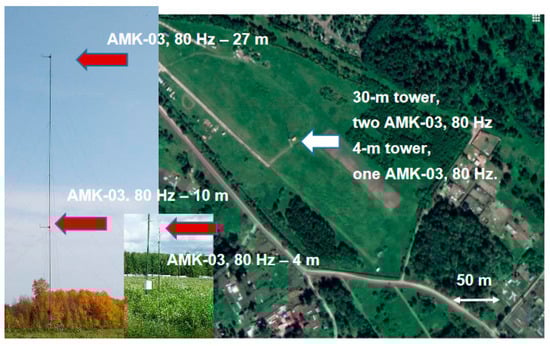
Figure 1.
Google map of the territory of the Basic Experimental Observatory and photographs of the 30 m and 4 m weather towers. Weather towers with acoustic anemometers installed on them at heights of 4, 10, and 27 m are located at the center of the Basic Experimental Observatory.

Table 1.
UAVs used in the experiment, the start and end time, the hover height, and wind speed.
Strictly speaking, the BEO territory is not a flat and uniform surface. The ground surface has a slope. It borders a villa community on one side and a forest on the other side. Earlier, we noted that turbulence over such a territory may deviate from isotropic [32].
The UAV measurements of the longitudinal and lateral wind velocities were calibrated during the experiment with the approach described in [32]. Table 2 presents the values of the calibration coefficients, average values of the longitudinal and lateral wind velocities and , and their standard deviations and in the hovering period.
Table 2.
Calibration coefficients, average values of the longitudinal and lateral wind velocity and , and their standard deviations and in the hovering period.
According to the data of the Tomsk International Airport located at a distance of ~10 km from BEO, the weather conditions observed during the experiment on 15 July 2021 were favorable in terms of quadcopter flight: south wind, speed of 5.0 m/s, air temperature of 17 °C, air humidity of 83%, horizontal visibility range of 10 km or more, and no precipitation. In contrast to the Tomsk International Airport data, the wind speed at the BEO territory was lower.
3. Results and Discussion
In this section, we consider the quadcopter velocity in the altitude hold mode. The behavior of this velocity allows us to judge how closely the experimental data correspond to ideal hovering. The longitudinal and lateral components of the wind velocity determined from the data of the quadcopters in the altitude hold mode are compared with the results of objective measurements by the AMK-03 anemometers. The correlation and spectral properties of atmospheric turbulence at different altitudes are analyzed, and the profiles of the longitudinal and transverse turbulence scales are studied.
3.1. Quadcopter Velocity
The theoretical model of ideal quadcopter hovering was proposed in [3,30,31,32]. One of the main principles of this model is that the components of the quadcopter velocity during hovering are equal to zero relative to the ground. According to this model, fluctuations of the longitudinal and lateral wind velocity components and the behavior of the turbulence spectra coincide with the reference data. However, the actual hover of a quadcopter in the atmosphere is not ideal, and the quadcopter may move along the axes x, y, and z during the experiment. Figure 2 shows the variations of the quadcopter velocity components relative to the ground along the x, y, and z axes during quadcopter hovering at altitudes of 4 (a), 10 (b), and 27 m (c) near AMK-03 anemometers installed on the weather towers. It can be seen that during the measurements, the quadcopter velocity components are equal to zero except for some periods of time. In these periods, the quadcopter velocity components are 0.1 m/s or 0.2 m/s, as can be seen from Figure 2.
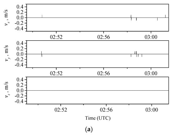
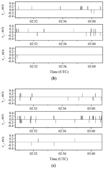
Figure 2.
Quadcopter velocity components along the x, y, and z axes during hovering; (a) 4 m, (b) 10 m, (c) 27 m.
As follows from [3,30,31,32], the deviation from the ideal hover leads to the appearance of high-frequency fluctuations in the fluctuations of the longitudinal and lateral wind components as compared to the reference data. However, despite the quadcopter hovering deviating from the ideal, the quadcopter data can be used to study the turbulence spectrum in the energy-containing and inertial ranges.
3.2. Longitudinal and Lateral Wind Velocity Components
Let us consider the behavior of the longitudinal and lateral components of the wind velocity estimated from the data of quadcopters in the altitude hold mode in the turbulent atmosphere in comparison with the reference results. Figure 3 shows the longitudinal and lateral wind velocity measured by the quadcopter (black curve) and AMK-03 anemometer (red curve) at heights of 4 (a, b), 10 (c, d), and 27 m (e, f). The top plot for each height corresponds to measurements in the 0–10 Hz band, while the bottom one is for the same data but smoothed for 1 min.
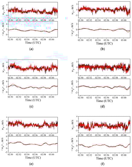
Figure 3.
Longitudinal and lateral wind velocities at a height of 4 (a,b), 10 (c,d), and 27 m (e,f); quadcopter (black curve) and AMK-03 acoustic anemometer (red curve) data. Top plots correspond to the values of and measured with a frequency of 10 Hz, bottom plots are for the 1 min smoothed data on and .
It is well known that the smoothing of random series leads to the averaging of high-frequency fluctuations. It can be seen from Figure 3 that the averaged data demonstrate the closest agreement between the UAV and AMK-03 data. Before the smoothing procedure, a significant discrepancy is observed in the data, including fluctuations in the 0–10 Hz frequency band.
The discrepancy between UAV and AMK-03 data before the smoothing procedure is characterized by the parameters and and, after the smoothing, by and . The series of and , as well as and , are random numbers whose scatter is characterized by
Table 3 gives the values of the variances at heights of 4, 10, and 27 m before and after the smoothing procedure. One can see that before the smoothing procedure, the variances are approximately m/s and m/s. After the smoothing of the measurement series, the variances decrease significantly down to m/s and m/s. Thus, the 1 min smoothing of the longitudinal and lateral wind velocities suppresses considerably high-frequency fluctuations, which leads to a significant decrease of the variances.
Table 3.
Variances , , and .
The variance is an integral characteristic of a random process. In contrast to the variance, the histogram and total probability in percent allows us to study the frequency distribution of random numbers and , as well as and . Figure 4 and Figure 5 show the histograms and total probabilities in percent for the discrepancy between the UAV and AMK-03 data before and after the smoothing procedure. It follows from Figure 4 that before the smoothing procedure, the discrepancy between the AMK-03 and quadcopter data does not exceed 0.7 m/s for the longitudinal component and ~1 m/s for the lateral component in 95% of cases (this level is shown by arrows in Figure 4 and Figure 5). After the 1 min smoothing of the measurement series, the discrepancy reduces significantly. Thus, for heights of 4 and 27 m, the discrepancy between the AMK-03 and quadcopter data does not exceed 0.5 m/s for both the longitudinal and lateral wind velocity components. For a height of 10 m, the discrepancy between the data ranges from 0 to 0.5 m/s in 95% of cases.
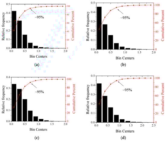
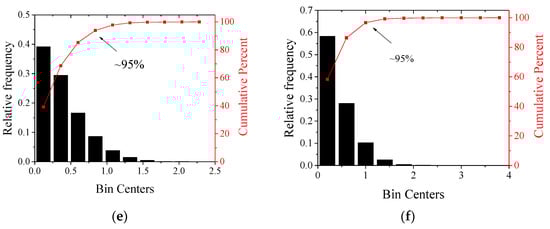
Figure 4.
Histograms and total probabilities in percent for the discrepancies between UAV and AMK-03 data for (a,c,e) and (b,d,f) before the smoothing procedure at a height of 4 (a,b), 10 (c,d), and 27 m (e,f).
Figure 5.
Histograms and total probabilities in percent for the discrepancies between UAV and AMK-03 data for (a,c,e) and (b,d,f) after the smoothing procedure at a height of 4 (a,b), 10 (c,d), and 27 m (e,f).
With 1 min averaging of the wind velocity components, insufficient smoothing of natural turbulent fluctuations of the wind velocity is observed [45], as can be seen from Figure 3. Aviation and other applications often use wind velocities averaged over this averaging time, and such results are treated as long turbulent gusts [45]. For many applications, the uncertainty of wind velocity measurements should not exceed 0.5 m/s for wind speeds less than 5 m/s [45]. These values are the most common meteorological requirements of the World Meteorological Organization for wind velocity measurements [45].
During our experiment, the wind speed at the heights under study did not exceed 5 m/s and the discrepancy did not exceed 0.5 m/s in 95% of cases for the longitudinal and lateral wind velocity components after the 1 min-smoothing procedure. Thus, a quadcopter swarm can provide the accuracy in determining the wind profile that meets the requirements of the World Meteorological Organization in the monitoring of long turbulent wind gusts [45].
3.3. Correlation Analysis
Let us analyze now the statistical correlation between the data measured with UAV and the AMK-03 acoustic anemometer. The correlation coefficient serves as a mathematical measure of the correlation between two random variables. Table 4 shows the values of the correlation coefficients for the longitudinal and lateral wind velocity components at heights of 4, 10, and 27 m before and after the smoothing procedure. We can see that the average values of the correlation coefficients before the smoothing procedure are, respectively, 0.71 and 0.66 for the longitudinal and lateral components. The 1 min smoothing leads to the average values of the correlation coefficients of 0.93 and 0.89, respectively, for the longitudinal and lateral components. Thus, the suppression of high-frequency fluctuations by applying the 1 min smoothing procedure to the series of longitudinal and lateral wind velocities leads to the significantly higher correlation manifesting itself in the higher correlation coefficient between the UAV and AMK-03 measurements.
Table 4.
Correlation coefficients.
Figure 6 shows the results of the calculation of the longitudinal and lateral autocorrelation functions of turbulent fluctuations of the wind velocity at heights of 4, 10, and 27 m. In addition to autocorrelation, of great interest is the cross-correlation between the quadcopter and AMK-03 acoustic anemometer data obtained at the same height. The behavior of cross-correlation functions of turbulent fluctuations at heights of 4, 10, and 27 m is shown in Figure 7.
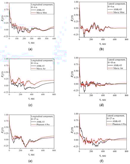
Figure 6.
Autocorrelation functions of longitudinal and lateral turbulent fluctuations of wind velocity at a height of 4 (a,b), 10 (c,d), and 27 m (e,f): AMK-03 anemometer (black curve) and UAV (red curve) data.
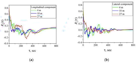
Figure 7.
Cross-correlation functions of turbulent fluctuations at a height of 4 (green curve), 10 (blue curve), and 27 m (red curve) for the longitudinal (a) and lateral (b) wind velocity components.
One can see that as increases, the autocorrelation for both UAV and AMK-03 data quickly drops down to zero and then oscillates around zero. The general behavior of the autocorrelation functions of longitudinal and lateral turbulent fluctuations of wind velocity for the two measurement methods coincides within the statistical uncertainty. It follows from Figure 7 that the cross-correlation also drops with time and then oscillates to zero. This behavior of autocorrelation and cross-correlation functions is typical for a turbulent atmosphere [44,46,47].
It is well-known [46,48] that oscillations of the autocorrelation functions around zero bear positive information about the state of the turbulent atmosphere. These oscillations are usually not studied because of the significant noise effect. It follows from Figure 6 that the noise effect may be insignificant in some cases, for example, (b) and (e), and far correlations coincide for the UAV and anemometer measurements. Thus, a quadcopter can be used to study far correlations, rather than in the range of small only.
3.4. Spectral Analysis
The spectra of turbulent wind velocity fluctuations were calculated by well-known methods using standard FFT software. It is known [33,34,35] that turbulence spectra change significantly with small variations of the frequency . These changes are random fluctuations about the main regularities of the turbulence spectra. To reveal these regularities in the turbulence spectra, a moving smoothing procedure over 50 points was used. We used this procedure for calculation of turbulence spectra in [3,30,31,32].
Figure 8 and Figure 9 show the calculated smoothed longitudinal and lateral spectra as judged from the quadcopter and AMK-03 anemometer data, and is the normalization coefficient. The green, blue, and red curves correspond to a height of 4, 10, and 27 m, respectively, while the black curve is the Kolmogorov–Obukhov turbulence spectrum. An analysis of the turbulence spectra shows that they coincide for the data measured with the quadcopters and acoustic anemometers at different heights, while differences are observed in the high-frequency spectral range of the spectrum. This behavior of the turbulence spectra measured by various methods was noted earlier in [3,30,31,32].
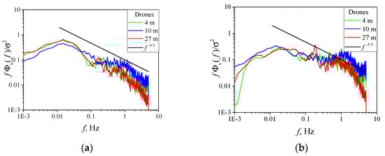
Figure 8.
Spectra of turbulent wind velocity fluctuations from quadcopter data at 4 (green curve), 10 (blue curve), and 27 m (red curve): (a) longitudinal and (b) lateral spectrum.
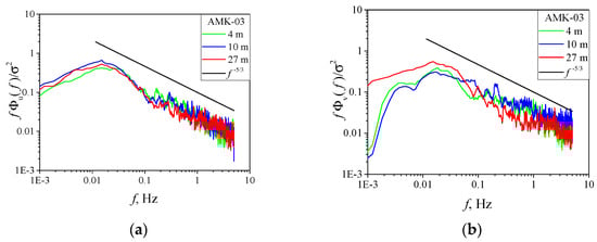
Figure 9.
Spectra of turbulent wind velocity fluctuations from AMK-03 anemometer data at 4 (green curve), 10 (blue curve), and 27 m (red curve): (a) longitudinal and (b) lateral spectrum.
3.5. Longitudinal and Lateral Scales of Turbulence
It is well-known that relative turbulence spectra contain information about the longitudinal and lateral scales of turbulence. The longitudinal and lateral turbulence scales were calculated based on Equations (3) and (4) for the von Karman model and Equations (7) and (8) for the Dryden model. The spectral maxima were determined from the smoothed experimental longitudinal and lateral spectra obtained from both the quadcopter and AMK-03 anemometer data. Table 5 presents the profiles of the longitudinal and lateral turbulence scales. The values calculated by the von Karman and Dryden models are separated by a slash. One can see from Table 5 that the values of the longitudinal turbulence scales coincide for both the quadcopter and AMK-03 anemometer data.
Table 5.
Profiles of the longitudinal and lateral turbulence scales for the von Karman model and Dryden model.
When analyzing the experimental data, a difference in the behavior of the ratio of turbulence scales from that in an isotropic atmosphere is marked. It follows from Table 5 that the experimentally measured value of the ratio of turbulence scales ranges from 0.59 to 0.74, whereas for isotropic turbulence. Thus, a deviation from the laws of isotropic turbulence was observed during the experiment.
We have noted earlier [32] that the same deviation from the laws of isotropic turbulence was observed in the experiment, which took place at the Basic Experimental Observatory. In the experiments [38,39], which were carried out for several years at the territory of the Tsimlyansk Research Station of the A.M. Obukhov Institute of Atmospheric Physics, it was found that the longitudinal scale, on average, exceeds the lateral scale 1.4 times or . The territories of the Basic Experimental Observatory and the Tsimlyansk Research Station have a nearly flat underlying surface. At such territories, slight deviations from isotropic turbulence can be observed, which is also confirmed by this study.
In contrast to a territory with a flat underlying surface, stronger deviations from isotropic turbulence can be observed in an urban environment [3]. For example, measurements of the ratio of turbulence scales for the urban environment in different seasons (winter, spring, summer, and fall) provide the ratios . Thus, the obtained results on the ratio of longitudinal and lateral turbulence scales are in agreement with the conclusions of [3,32,38,39].
During the experiment, the quadcopter was at a distance of ~5 m from the acoustic anemometer. This distance was chosen from safety reasons for the experiment. Let us estimate the drop in the correlation of the wind velocity field at a distance of ~5 m using the Dryden model (9) and (10). It follows from Table 5 that the turbulence scales varied from 10 to 17 m depending on the height. This relation of the turbulence scales and the distance from the acoustic anemometer to the quadcopter means that the instruments were within the same turbulent structure, within which an air vortex moves almost synchronously.
The calculations show that the average values of the correlation function for two points spaced by 5 m are 0.8 for the longitudinal wind velocity and 0.6 for the lateral wind velocity. Thus, during the experiment, the instruments were within the same turbulent structure, but at a significant distance. Thus, we can only approximately speak about the synchronism of motion inside the air vortex. The problems with calibration when field data are used, which are discussed in detail in [36,37], may be due to the decreasing correlation in the wind velocity field with an increase in the distance between the UAV and the anemometer. The complex airflow in the atmosphere and, as a consequence, partial synchronism of turbulent vortices, can lead to large errors, as indicated in [36,37].
The results of measurements of the autocorrelation functions allow us to estimate the longitudinal and lateral turbulence scales. These scales were estimated by the least square fit method with the Dryden model as the best fit curve. The longitudinal and lateral correlation functions of this model have a simple analytical form described by Equations (9) and (10). The turbulence scales are the best fit coefficients when this method is used. Also in [3], the least square fit method was applied to estimate the turbulence scales with the turbulence spectra used as the best-fit curve. The Dryden model qualitatively describes the state of atmospheric turbulence, so its use allows the longitudinal and lateral scales to be estimated only qualitatively. Table 6 provides the estimates of the longitudinal and lateral scales of turbulence obtained by the least square fit method. The comparison of and in Table 5 and Table 6 shows that they coincide in the order of magnitude.
Table 6.
Longitudinal and lateral scales of turbulence.
4. Conclusions
Atmospheric turbulence is a random medium, in which the wind velocity field varies significantly in space. The turbulent wind velocity field experiences the strongest variations in the vertical direction. Therefore, of great scientific and practical interest is monitoring of the vertical profile of turbulence with quadcopters in the hovering mode, which can provide high spatial resolution in atmospheric monitoring. In contrast to [3,30,31,32], in which atmospheric turbulence was studied based on spectral analysis, this paper presents the results of both spectral and correlation analysis in the monitoring of the vertical turbulence profile.
The profile of atmospheric turbulence was measured at the territory of the Basic Experimental Observatory (Tomsk, Russian Federation) at altitudes of 4, 10, and 27 m using both quadcopters and AMK-03 acoustic anemometers. In the experiment, the behavior of the longitudinal and lateral components of the wind velocity was studied, and the discrepancy between the quadcopter and AMK-03 data before and after the smoothing procedure was analyzed. The spectral and correlation analysis of the quadcopter and anemometer findings was carried out. The profiles of the longitudinal and lateral scales of turbulence were studied.
It is shown that the quadcopter and anemometer data measured in the 0–10 Hz frequency band have a discrepancy in the high-frequency spectral range, but are in agreement after 1 min of averaging. Before the smoothing procedure, the variances for the longitudinal and lateral wind velocity are about ~0.45 m/s, while the smoothing of the measurement series reduces them down to ~0.15 m/s. The analysis of the histograms and total probabilities of the discrepancies between the UAV and AMK-03 data allows us to state that during the experiment, the discrepancy did not exceed 0.5 m/s in 95% of cases for the longitudinal and lateral wind velocity components after the 1 min smoothing procedure. The correlation coefficients for the longitudinal and lateral components increase considerably from ~0.71 to ~0.9 after the smoothing procedure.
The calculations of the autocorrelation and cross-correlation functions, as well as turbulence spectra obtained from the quadcopter and anemometer data, show the behavior typical for a turbulent atmosphere [44,46,47]. The comparison of the longitudinal and lateral turbulence scales obtained from the quadcopter and anemometer data suggests that they coincide within the statistical uncertainty for the different methods of determining these parameters.
The analysis of the data obtained revealed a deviation from the laws of isotropic turbulence during the experiment: the measured ratio of the turbulence scales ranges from 0.59 to 0.74, whereas it should be 0.5 for isotropic turbulence. This behavior of the turbulence scale ratio is in agreement with the data of [38,39] obtained over several years at the territory of the Tsimlyansk Scientific Station of the A.M. Obukhov Institute of Atmospheric Physics, as well as with the results of the experiment in an urban environment [3].
Based on the results obtained, we can conclude that a swarm of quadcopters is a promising tool for determining atmospheric turbulence profiles with high spatial resolution. The use of several rotary wing UAVs in the hover mode can allow a detailed description of the state of turbulence, which significantly impacts many processes occurring in the atmosphere. Detailed description of the state of atmospheric turbulence is very important for solving numerous problems, including navigation of drones under adverse meteorological conditions over territories with complex orography, such as urban environments and various types of natural landscapes, as well as in hard-to-reach or dangerous places.
Author Contributions
Conceptualization, A.S.; methodology, A.S.; software, A.A. and E.S.; validation, A.K., A.T. and A.M.; investigation, A.S. and A.A.; data curation, A.K., A.T. and A.M.; writing—original draft preparation, O.P.; writing—review and editing, A.S.; supervision, A.S.; project administration, A.S. All authors have read and agreed to the published version of the manuscript.
Funding
The study was supported by the Russian Foundation for Basic Research (project no. 19-29-06066 mk).
Data Availability Statement
The data presented in this study are available on request from the corresponding author.
Acknowledgments
The authors are grateful to A.B. Gonchar for the help in preparing this paper.
Conflicts of Interest
The authors declare no conflict of interest. The funders had no role in the design of the study; in the collection, analyses, or interpretation of data; in the writing of the manuscript; or in the decision to publish the results.
References
- Cornman, L.B.; Chan, W.N. Summary of a workshop on integrating weather into unmanned aerial system traffic management. Bull. Am. Meteorol. Soc. 2017, 98, ES257–ES259. [Google Scholar] [CrossRef]
- Beard, R.; McLain, T. Small Unmanned Aircraft: Theory and Practice; Princeton University Press: Princeton, NJ, USA, 2010. [Google Scholar]
- Shelekhov, A.; Afanasiev, A.; Shelekhova, E.; Kobzev, A.; Tel’minov, A.; Molchunov, A.; Poplevina, O. Low-Altitude Sensing of Urban Atmospheric Turbulence with UAV. Drones 2022, 6, 61. [Google Scholar] [CrossRef]
- Kral, S.T.; Reuder, J.; Vihma, T.; Suomi, I.; O’Connor, E.; Kouznetsov, R.; Wrenger, B.; Rautenberg, A.; Urbancic, G.; Jonassen, M.O.; et al. Innovative strategies for observations in the arctic atmospheric boundary layer (ISOBAR)—The Hailuoto 2017 campaign. Atmosphere 2018, 9, 268. [Google Scholar] [CrossRef]
- Stith, J.L.; Baumgardner, D.; Haggerty, J.; Hardesty, M.; Lee, W.; Lenschow, D.; Pilewskie, P.; Smith, P.L.; Steiner, M.; Vömel, H. 100 Years of progress in atmospheric observing systems. Meteorol. Monogr. 2018, 59, 2.1–2.55. [Google Scholar] [CrossRef]
- Hocking, W.K.; Röttger, J.; Palmer, R.D.; Sato, T.; Chilson, P.B. Atmospheric Radar; Cambridge University Press: Cambridge, UK, 2016. [Google Scholar]
- Leosphere, Windcube, Vaisala. Available online: https://www.vaisala.com/en/wind-lidars/wind-energy/windcube/ (accessed on 30 April 2023).
- METEK Meteorologische Messtechnik GmbH. Available online: https://metek.de/product-group/doppler-sodar/ (accessed on 30 April 2023).
- Scintec. Available online: https://www.scintec.com/ (accessed on 30 April 2023).
- Zhu, B.; Qunbo, L.; Tan, Z. Adaptive Multi-Scale Fusion Blind Deblurred Generative Adversarial Network Method for Sharpening Image Data. Drones 2023, 7, 96. [Google Scholar] [CrossRef]
- Xiao, Y.; Zhang, J.; Chen, W.; Wang, Y.; You, J.; Wang, Q. SR-DeblurUGAN: An End-to-End Super-Resolution and Deblurring Model with High Performance. Drones 2022, 6, 162. [Google Scholar] [CrossRef]
- Tajima, Y.; Hiraguri, T.; Matsuda, T.; Imai, T.; Hirokawa, J.; Shimizu, H.; Kimura, T.; Maruta, K. Analysis of Wind Effect on Drone Relay Communications. Drones 2023, 7, 182. [Google Scholar] [CrossRef]
- Commission for Basic Systems and Commission for Instruments and Methods of Observation: Workshop on Use of Unmanned Aerial Vehicles (UAV) for Operational Meteorology WMO. 2019. Available online: https://library.wmo.int/doc_num.php?explnum_id=9951 (accessed on 30 April 2023).
- AMDAR Reference Manual: Aircraft Meteorological Data Relay WMO-No. 958, WMO. 2003. Available online: https://library.wmo.int/doc_num.php?explnum_id=9026 (accessed on 30 April 2023).
- Stoffelen, A.; Benedetti, A.; Borde, R.; Dabas, A.; Flamant, P.; Forsythe, M.; Hardesty, M.; Isaksen, L.; Källén, E.; Körnich, H.; et al. Wind Profile Satellite Observation Requirements and Capabilities. Bull. Amer. Meteor. Soc. 2020, 101, E2005–E2021. [Google Scholar] [CrossRef]
- Liao, X.; Xu, C.; Ye, H.; Tan, X.; Fang, S.; Huang, Y.; Lin, J. Critical Infrastructures for Developing UAVs’ Applications and Low-altitude Public Air-Route Network Planning. Bull. Chin. Acad. Sci. (Chin. Version) 2022, 37, 977–988. [Google Scholar]
- González-Rocha, J.; Bilyeu, L.; Ross, S.D.; Foroutan, H.; Jacquemin, S.J.; Ault, A.P.; Schmale, D.G., III. Sensing atmospheric flows in aquatic environments using a multirotor small unscrewed aircraft system (sUAS). Environ. Sci. Atmos. 2023, 3, 305–315. [Google Scholar] [CrossRef]
- Lepikhin, A.P.; Lyakhin, Y.S.; Lucnikov, A.I. The Experience in Drone Use to Evaluate the Coefficients of Turbulent Diffusion in Small Water Bodies. Water Resour. 2023, 50, 242–251. [Google Scholar] [CrossRef]
- McConville, A.; Richardson, T. High-altitude vertical wind profile estimation using multirotor vehicles. Front. Robot. AI 2023, 10, 1112889. [Google Scholar] [CrossRef] [PubMed]
- Villa, T.F.; Gonzalez, F.; Miljievic, B.; Ristovski, Z.D.; Morawska, L. An Overview of Small Unmanned Aerial Vehicles for Air Quality Measurements: Present Applications and Future Prospectives. Sensors 2016, 16, 1072. [Google Scholar] [CrossRef] [PubMed]
- Loubimov, G.; Kinzel, M.P.; Bhattacharya, S. Measuring Atmospheric Boundary Layer Profiles Using UAV Control Data. In Proceedings of the AIAA Scitech 2020 Forum, Orlando, FL, USA, 6–10 January 2020; American Institute of Aeronautics and Astronautics: Orlando, FL, USA, 2020. [Google Scholar] [CrossRef]
- Li, Z.; Pu, O.; Pan, Y.; Huang, B.; Zhao, Z.; Wu, H. A Study on Measuring the Wind Field in the Air Using a Multi-rotor UAV Mounted with an Anemometer. Bound.-Layer Meteorol. 2023, 188, 1–27. [Google Scholar] [CrossRef]
- González-Rocha, J.; De Wekker, S.F.J.; Ross, S.D.; Woolsey, C.A. Wind Profiling in the Lower Atmosphere from Wind-Induced Perturbations to Multirotor UAS. Sensors 2020, 20, 1341. [Google Scholar] [CrossRef]
- González-Rocha, J.; Woolsey, C.A.; Sultan, C.; De Wekker, S.F.J. Sensing wind from quadrotor motion. J. Guid. Control Dyn. 2019, 42, 836–852. [Google Scholar] [CrossRef]
- González-Rocha, J.; Woolsey, C.A.; Sultan, C.; De Wekker, S.F. Model-based wind profiling in the lower atmosphere with multirotor UAS. In Proceedings of the AIAA Scitech 2019 Forum, San Diego, CA, USA, 7–11 January 2019; p. 1598. [Google Scholar]
- Neumann, P.; Bartholmai, M. Real-time wind estimation on a micro unmanned aerial vehicle using its inertial measurement unit. Sens. Actuators A Phys. 2015, 235, 300–310. [Google Scholar] [CrossRef]
- Palomaki, R.T.; Rose, N.T.; van den Bossche, M.; Sherman, T.J.; De Wekker, S.F.J. Wind estimation in the lower atmosphere using multirotor aircraft. J. Atmos. Ocean. Technol. 2017, 34, 1183–1190. [Google Scholar] [CrossRef]
- Meier, K.; Hann, R.; Skaloud, J.; Garreau, A. Wind Estimation with Multirotor UAVs. Atmosphere 2022, 13, 551. [Google Scholar] [CrossRef]
- Cheng, X.; Wang, Y.; Cai, Z.; Liu, N.; Zhao, J. Wind Estimation of a Quadrotor Unmanned Aerial Vehicle. In Advances in Guidance, Navigation and Control; ICGNC 2022 Lecture Notes in Electrical Engineering; Yan, L., Duan, H., Deng, Y., Eds.; Springer: Singapore, 2023; Volume 845. [Google Scholar] [CrossRef]
- Shelekhov, A.P.; Afanasiev, A.L.; Kobzev, A.A.; Shelekhova, E.A. Opportunities to monitor the urban atmospheric turbulence using unmanned aerial system. In Remote Sensing Technologies and Applications in Urban Environments V; SPIE: Washington, DC, USA, 2020; Volume 11535, p. 1153506. [Google Scholar] [CrossRef]
- Shelekhov, A.P.; Afanasiev, A.L.; Shelekhova, E.A.; Kobzev, A.A.; Tel’minov, A.E.; Molchunov, A.N.; Poplevina, O.N. Profiling the turbulence from spectral measurements in the urban atmosphere using UAVs. In Remote Sensing Technologies and Applications in Urban Environments VI; SPIE: Washington, DC, USA, 2021; Volume 11864, p. 118640B. [Google Scholar] [CrossRef]
- Shelekhov, A.; Afanasiev, A.; Shelekhova, E.; Kobzev, A.; Tel’minov, A.; Molchunov, A.; Poplevina, O. Using small unmanned aerial vehicles for turbulence measurements in the atmosphere. Izv. Atmos. Ocean. Phys. 2021, 57, 533–545. [Google Scholar] [CrossRef]
- Monin, A.S.; Yaglom, A.M. Statistical Hydromechanics. Part 2. In Turbulent Mechanics; Nauka: Moscow, Russia, 1967. [Google Scholar]
- Stull, R.B. An Introduction to Boundary Layer Meteorology; Kluwer Academic Publishers: Dordrecht, The Netherlands, 1989. [Google Scholar]
- Kaimal, J.C.; Finnigan, J.J. Atmospheric Boundary Layer Flows: Their Structure and Measurement; Oxford University Press: Oxford, UK, 1994. [Google Scholar]
- Wildmann, N.; Wetz, T. Towards vertical wind and turbulent flux estimation with multicopter uncrewed aircraft systems. Atmos. Meas. Tech. 2022, 15, 5465–5477. [Google Scholar] [CrossRef]
- Wetz, T.; Wildmann, N. Spatially distributed and simultaneous wind measurements with a fleet of small quadrotor UAS. J. Phys. Conf. Ser. 2022, 2265, 022086. [Google Scholar] [CrossRef]
- Shishov, E.A.; Solenaya, O.A.; Chkhetiani, O.G.; Azizyan, G.V.; Koprov, V.M. Multipoint measurements of temperature and wind in the surface layer. Izv. Atmos. Ocean. Phys. 2021, 57, 254–263. [Google Scholar] [CrossRef]
- Shishov, E.A.; Solyonaya, O.A.; Koprov, B.M.; Koprov, V.M. Investigation into variations of wind directions near the surface. Izv. Atmos. Ocean. Phys. 2018, 54, 515–523. [Google Scholar] [CrossRef]
- Azbukin, A.A.; Bogushevich, A.Y.; Korolkov, V.A.; Tikhomirov, A.A.; Shelevoi, V.D. A field version of the AMK-03 automated ultrasonic meteorological complex. Russ. Meteorol. Hydrol. 2009, 34, 133–136. [Google Scholar] [CrossRef]
- Azbukin, A.A.; Bogushevich, A.Y.; Kobzev, A.A.; Korolkov, V.A.; Tikhomirov, A.A.; Shelevoy, V.D. AMK-03 Automatic weather stations, their modifications and applications. Sens. Syst. 2012, 3, 47–52. [Google Scholar]
- McCombs, A.G.; Hiscox, A.L. Always in flux: The nature of turbulence. In Conceptual Boundary Layer Meteorology; Hiscox, A.L., Ed.; Academic Press: Cambridge, MA, USA, 2023; pp. 19–35. [Google Scholar] [CrossRef]
- Tieleman, H.W. Universality of velocity spectra. J. Wind Eng. Ind. Aerodyn. 1995, 56, 55–69. [Google Scholar] [CrossRef]
- Flay, R.G.J.; Stevenson, D.C. Integral length scales in an atmospheric boundary-layer near the Ground. In Proceedings of the 9th Australasian Fluid Mechanics Conference, Auckland, New Zealand, 8–12 December 1986. [Google Scholar]
- Guide to Instruments and Methods of Observation Volume I—Measurement of Meteorological Variables (WMO-No. 8) WMO; WMO: Geneva, Switzerland, 2021.
- O’Neill, P.L.; Nicolaides, D.; Honnery, D.; Soria, J. Autocorrelation Functions and the Determination of Integral Length with Reference to Experimental and Numerical Data. In Proceedings of the 15th Australasian Fluid Mechanics Conference, Sydney, Australia, 13–17 December 2004. [Google Scholar]
- Emes, M.J.; Arjomandi, M.; Kelso, R.M.; Ghanadi, F. Integral length scales in a low-roughness atmospheric boundary layer. In Proceedings of the 18th Australasian Wind Engineering Society Workshop, McLaren Vale, Australia, 6–8 July 2016; pp. 1–4. [Google Scholar]
- Yaglom, A.M. Correlation Theory of Stationary and Related Random Functions, Volume 1: Basic Results; Springer: Berlin/Heidelberg, Germany, 1987. [Google Scholar]
Disclaimer/Publisher’s Note: The statements, opinions and data contained in all publications are solely those of the individual author(s) and contributor(s) and not of MDPI and/or the editor(s). MDPI and/or the editor(s) disclaim responsibility for any injury to people or property resulting from any ideas, methods, instructions or products referred to in the content. |
© 2023 by the authors. Licensee MDPI, Basel, Switzerland. This article is an open access article distributed under the terms and conditions of the Creative Commons Attribution (CC BY) license (https://creativecommons.org/licenses/by/4.0/).