Geometric and Radiometric Quality Assessments of UAV-Borne Multi-Sensor Systems: Can UAVs Replace Terrestrial Surveys?

Abstract

Unmanned aerial vehicles (UAVs), also known as drones, are a cost-effective alternative to traditional surveying methods, and they can be used to collect geospatial data over inaccessible or hard-to-reach locations. UAV-integrated miniaturized remote sensing sensors such as hyperspectral and LiDAR sensors, which formerly operated on airborne and spaceborne platforms, have recently been developed. Their accuracies can still be guaranteed when incorporating pieces of equipment such as ground control points (GCPs) and field spectrometers. This study conducted three experiments for geometric and radiometric accuracy assessments of simultaneously acquired RGB, hyperspectral, and LiDAR data from a single mission. Our RGB and hyperspectral data generated orthorectified images based on direct georeferencing without any GCPs. Because of this, a base station is required for the post-processed Global Navigation Satellite System/Inertial Measurement Unit (GNSS/IMU) data. First, we compared the geometric accuracy of orthorectified RGB and hyperspectral images relative to the distance of the base station to determine which base station should be used. Second, point clouds could be generated from overlapped RGB images and a LiDAR sensor. We quantitatively and qualitatively compared RGB and LiDAR point clouds in this experiment. Lastly, we evaluated the radiometric quality of hyperspectral images, which is the most critical factor of the hyperspectral sensor, using reference spectra that was simultaneously measured by a field spectrometer. Consequently, the distance of the base station for post-processing the GNSS/IMU data was found to have no significant impact on the geometric accuracy, indicating that a dedicated base station is not always necessary. Our experimental results demonstrated geometric errors of less than two hyperspectral pixels without using GCPs, achieving a level of accuracy that is comparable to survey-level standards. Regarding the comparison of RGB- and LiDAR-based point clouds, RGB point clouds exhibited noise and lacked details; however, through the cleaning process, their vertical accuracy was found to be comparable with LiDAR’s accuracy. Although photogrammetry generated denser point clouds compared with LiDAR, the overall quality for extracting the elevation data greatly relies on factors such as the original image quality, including the image’s occlusions, shadows, and tie-points, for matching. Furthermore, the image spectra derived from hyperspectral data consistently demonstrated high radiometric quality without the need for in situ field spectrum information. This finding indicates that in situ field spectra are not always required to guarantee the radiometric quality of hyperspectral data, as long as well-calibrated targets are utilized.

1. Introduction

Increased interests in remote sensing and unmanned aerial vehicles (UAVs), which are motivated by a desire to detect and characterize detailed information about targets of interest, have led to the development of advanced and miniaturized sensors. In recent years, the amount of high-resolution geospatial data acquired from UAVs has significantly increased to replicate the real world into the digital space and find a solution for the real-world problems that we are facing [1]. Moreover, integrating multiple sensor-based data can provide an improved capacity for exploiting practical remote sensing applications [2,3].

A digital camera is the most basic and simplest type of UAV instrument. Although it is cheap, easy to process, and provides relatively high-resolution images, it is challenging for it to provide scientifically meaningful information. On the other hand, high spectral resolution sensors in hundreds of spectral bands of narrow bandwidths enhance the capability to identify materials compared with multispectral sensors [4]. Hyperspectral images are generally acquired from airborne (e.g., Airborne Visible/Infrared Imaging Spectrometer (AVIRIS) [5]) or spaceborne (e.g., Hyperion [6], PRecursore IperSpettrale della Missione Applicativa (PRISMA) [7]) platforms. However, recent advances in sensor technologies have led to the development of miniaturized hyperspectral sensors for UAV platforms [8]. Light detection and ranging (LiDAR) technology, which measures the range, position, and attitude to determine three-dimensional coordinates accurately, has been widely used in various applications, such as agriculture, forest, mobility, and urban applications, due to it being an accurate, efficient, and low-cost surveying scheme. Airborne LiDAR systems were commonly used to map extended areas with a relatively low point density; UAV-borne LiDAR systems at a low altitude are emerging as an alternative to field surveys. Multi-modal remote sensing data refer to the use of different types of sensor data, and this method generally allows for a more comprehensive and accurate understanding of the Earth’s surface than either data type alone [2,3]. Simultaneously acquired data from the integrated multi-sensor systems can be easily associated with each other as they observe the same status of the ground targets if they are able to guarantee geometric and radiometric quality.

The widely used Global Navigation Satellite System/Inertial Measurement Unit (GNSS/IMU) of UAVs has a few meters of positioning errors [9]. The digital numbers of optical sensors (e.g., RGB, multispectral, or hyperspectral) have no physical meanings. A quantitative analysis can be limited for practical and scientific applications without correcting for the geometric errors and conversions from digital numbers to physical units. Although UAV-borne geospatial data acquisitions should be easy and fast, additional field surveys using geometric/radiometric targets and instruments in order to guarantee geometric and radiometric quality are still costly. As an alternative, the use of survey-level GNSS/IMU and diffuse reflectance targets may reduce efforts for field surveys and help to obtain high-quality scientific data.

This study evaluated the geometric and radiometric quality of GNSS/IMU-assisted RGB, hyperspectral, and LiDAR sensor data that were simultaneously acquired from a small UAV to establish more efficient UAV data acquisitions and potential applications. Three experiments were carried out: (1) Survey-level GNSS/IMU data can be processed using dedicated base station data or using GNSS data providing services such as continuously operating reference stations (CORSs). In general, the closer the base station, the better the accuracy. In this experiment, we investigated the geometric accuracies according to the distance of the base station and then determined whether the on-site base station was required. (2) The vertical information of the ground targets is helpful for industrial/scientific applications and essential for generating orthorectified images. Point clouds can be obtained from both LiDAR and overlapped RGB images. This experiment aimed to compare LiDAR and RGB point clouds qualitatively and quantitatively using three-dimensional objects. (3) Hyperspectral sensors record reflected radiation from a ground target over a continuous range of wavelengths and detect the individual absorption features that are related to specific chemical bonds [4,9,10,11]. Therefore, radiometric quality and stability are critical for determining the performance of hyperspectral sensors. In this experiment, we compared image-derived spectra with the ground truth data that were simultaneously measured using a field spectrometer.

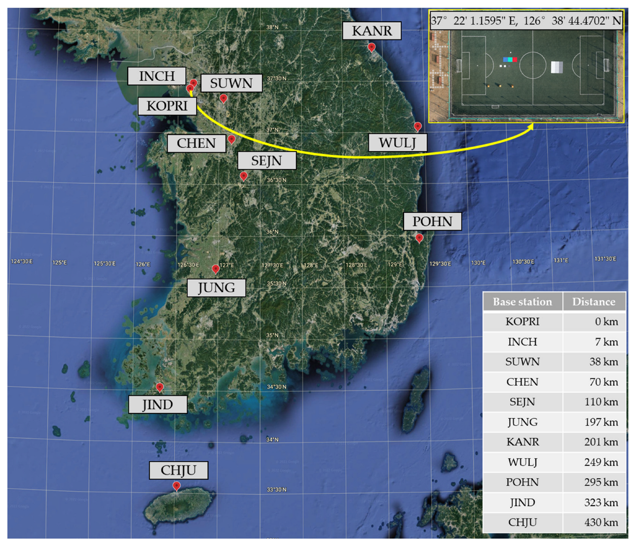
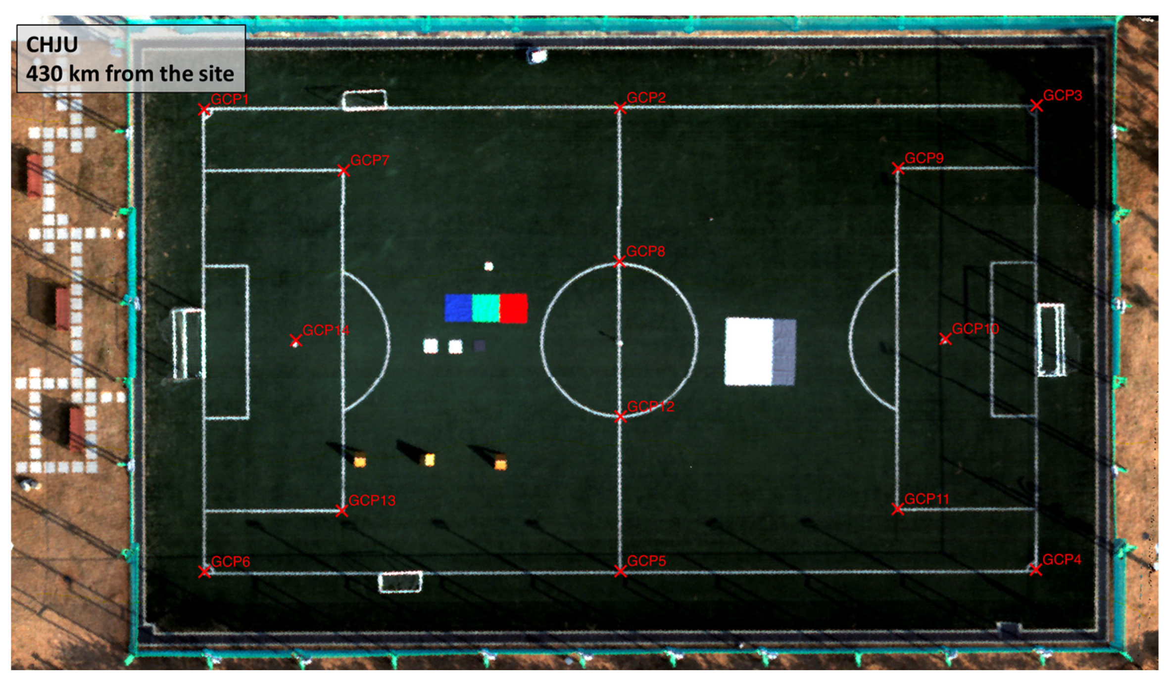
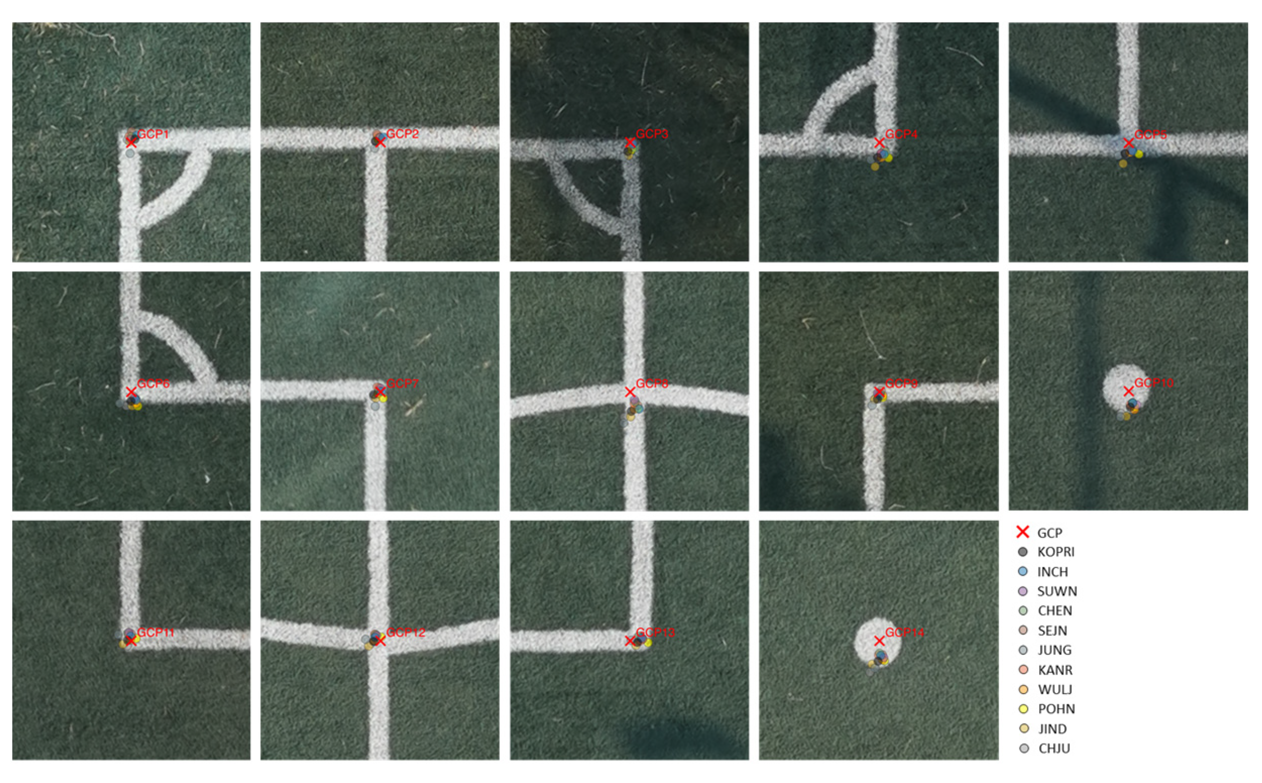
2. Data Acquisitions

We acquired RGB, hyperspectral, and LiDAR data using an integrated multi-sensor system onboard a DJI Matrice 600 Pro drone (Figure 1) on 26 January 2022 over a playground in Incheon, Korea (37°22′1.1595″ E; 126°38′44.4702″ N). The datasheet of each sensor is presented in

Table 1. Datasheet of the RGB, hyperspectral, and LiDAR sensor.

RGB (SONY A7R III)
Spatial pixels (image size)	7952 × 5304
Sensor size	35.943 mm × 23.974 mm
Detector pixel size	4.52 µm
Focal length	35 mm
Hyperspectral (Headwall Nano-Hyperspec)
Spectral range	400–1000 nm
Spectral pixels (or bands)	270
Detector pixel size	7.4 µm
Spatial pixels	640
Charge-coupled device (CCD) technology	Complementary metal oxide semiconductor (CMOS)
Maximum frame rate	350 Hz
Pixel depth (dynamic range)	12-bit
Focal length of lens	8 mm
LiDAR (Velodyne Puck Hi-Res)
Number of channels	16
Maximum measurement range	100 m
Range accuracy (typical)	Up to ±3 cm
Field of view	−10°–10° (vertical); 360° (horizontal)
Angular resolution	1.33° (vertical); 0.1°–0.4° (horizontal)
Rotation rate	5–20 Hz
Laser wavelength	903 nm
Laser pulses per second	300,000 (single return mode) 600,000 (dual return mode)

.

Ground control points (GCPs) are often deployed and surveyed to provide accurate positions, but they are costly. To accurately provide the position and orientation of the sensors for direct georeferencing without GCPs, a survey-grade GNSS/IMU, the Trimble APX-15 system, was integrated with the remote sensing sensors. Applanix’s differential GNSS-aided inertial post-processing software, POSPac UAV, generated more accurate post-processed kinematic (PPK) data than standard positioning service (SPS). The expected errors are 0.02–0.05 m for a position, 0.015 m/s for the velocity, 0.025° for the roll and pitch angles, and 0.08° for the heading, which are significantly more accurate results than SPS (e.g., 1.5–3.0 m for a position, 0.05 m/s for the velocity, 0.04° for the roll and pitch angles, and 0.3° for heading) [12]. Especially, PPK data are essential for the pushbroom hyperspectral sensor, which requires the exterior orientation parameters for every scan line [13], and for LiDAR, which determines three-dimensional coordinates using the position and attitude [14].

For geometric and radiometric quality assessments of RGB, hyperspectral, and LiDAR sensors, we deployed several targets or used existing objects in the soccer field, as shown in Figure 2. First, the exposure time and frame period of the hyperspectral sensor were determined based on the illumination conditions to acquire the best radiometric quality hyperspectral images. Flight speed and altitude were then determined. We obtained data from four flight lines at a flight speed of 3 m/s and an altitude of 44 m. As a result, the ground sample distance (GSD) of the RGB and hyperspectral images was approximately 0.6 cm and 4 cm, respectively. The LiDAR point density from a single pass was approximately 316 points/m².

3. Methods

Figure 3 illustrates a brief workflow of this study. To evaluate positioning errors (see red rectangles in Figure 3), we first compared the non-PPK system with the PPK system using orthomosaic images from RGB images. Then, we investigated the impact of the distance of the CORSs for the PPK using hyperspectral images. For the second experiment, point clouds generated from RGB and LiDAR data were quantitatively and qualitatively evaluated (see the blue rectangle in Figure 3). Lastly, the radiometric quality of the hyperspectral images was determined with respect to the wavelength and flight passes (see the green rectangle in Figure 3).

In our data processing workflow, we used PIX4Dmapper software to process the RGB point clouds and orthomosaic images while using our custom code to generate the LiDAR point clouds and orthomosaic processing of the hyperspectral data. The technical details of our code are described in [13,15].

3.1. Position Accuracy of Orthorectified Images

In this experiment, we compared the geometric accuracy of the orthorectified images acquired from the RGB and hyperspectral sensors according to the distance of the base station. First, we selected 14 corners or intersections of soccer field lines as GCPs (Figure 2). To survey these points, we used a Trimble R8 as a rover. The rover received real-time kinematic (RTK) corrections from a network RTK service that was provided by the National Geographic Information Institute in Korea; this allowed for the high-accuracy positioning of the GCPs, and the results are listed in

Table 2. Ground coordinates of 14 ground control points (GCPs) (UTM Zone 52N, unit: m).

GCP	X	Y	GCP	X	Y
#1	291,510.212	4,138,204.498	#8	291,520.020	4,138,188.103
#2	291,524.214	4,138,193.245	#9	291,531.900	4,138,183.662
#3	291,538.254	4,138,182.009	#10	291,528.850	4,138,176.649
#4	291,525.611	4,138,166.438	#11	291,522.622	4,138,172.227
#5	291,511.632	4,138,177.683	#12	291,515.831	4,138,182.864
#6	291,497.650	4,138,188.961	#13	291,503.926	4,138,187.281
#7	291,513.239	4,138,198.653	#14	291,507.010	4,138,194.246

.

As a baseline for investigating the nominal geometric errors of widely used UAV platforms, we acquired images from a DJI Phantom 4, which is a non-RTK- or PPK-supported platform. For the PPK, the Receiver Independent Exchange Format (RINEX) files from the CORSs are easy to access. However, the positioning accuracy generally drops as the distance between the rover and base station increases. The number of CORSs in remote places such as deserts, oceans, and polar regions is less than those in areas of civilization. The operation of a dedicated on-site base station may be ideal, but it is costly and difficult to determine an accurate location. Therefore, we used a Trimble R8 receiver as a dedicated base station and selected ten CORSs in Korea as reference stations, as shown in Figure 4, to compare the impact on the geometric accuracy relative to the rover–base distance.

We used individually orthorectified hyperspectral images in this experiment. Because the hyperspectral sensor is a pushbroom scanner, it requires exterior orientation parameters (EOPs), which can be determined from the PPK data for every scan line. Subtle differences in the boresight angles and lever-arm offsets of the sensor systems are critical to the quality of orthorectified hyperspectral images [13,15]. We used precisely estimated boresight angles and lever-arm offsets. Because the digital surface model (DSM) over the mission area is also crucial to the successful orthorectification of hyperspectral data, we used a DSM that was generated by LiDAR point clouds.

3.2. Quality and Vertical Accuracy of RGB and LiDAR Point Clouds

Although point clouds can be generated using LiDAR, photogrammetry using overlapped RGB images can be considered as an alternative. This experiment compared the visual and statistical accuracy between RGB- and LiDAR-generated point clouds. First, we generated RGB and LiDAR point clouds using the PPK data processed by the on-site base station. Then, we used three types of ground objects: two soccer goals, two futsal goals, and three A-frame signs (yellow rectangles in Figure 2). We measured the heights of the targets using a ruler and calculated the average size of each type of target. Because selecting the bottom/top of the targets from thousands of three-dimensional points may contain uncertainties, we used histograms of the targets for more generalized point picking, as shown in Figure 5.

3.3. Radiometric Quality of Hyperspectral Images

Because the use of hyperspectral sensors, also known as imaging spectroscopy, records the reflected radiation from a ground target using continuous spectral bands, radiometric similarity with ground truth spectra should be guaranteed before using hyperspectral sensors. The raw image pixels of hyperspectral sensors are not physically meaningful values, and they should be converted to radiance or reflectance data. Two radiometric processing steps are usually imposed: (1) converting raw digital numbers to radiance and (2) converting radiance to reflectance. For the first step, the sensor collects dark reference images under light-free conditions using a lens cover before or after a flight; it removes the dark current and calculates radiance values using the calibration data provided by the manufacturer [11,15,16]. For a quantitative analysis, radiance is then typically converted to reflectance, which is the fraction of incident electromagnetic energy as a function of the wavelength. The empirical linear regression uses spectrally uniform and known ground targets. The use of the ground truth spectra of the calibration targets collected during the flight for the development of regression models may be ideal. Nevertheless, it is time-consuming and requires an expensive field spectrometer. This study used spectrally uniform radiometric targets and their laboratory spectra for converting to reflectance values. We deployed nine radiometric calibration targets, as shown in the blue rectangles in Figure 2 and Figure 6, and also used artificial turf for the radiometric quality assessments. Two types of radiometric targets were used. We used six fabric radiometric tarps (11%, 30%, and 56% of gray, red, green, and blue), which were constructed using lightweight woven polyester (Group 8 Technology Inc., UT, USA). The sizes of each of the gray and color scale targets were 1 × 3 m and 1 × 1 m, respectively. We also deployed three non-fabric diffuse targets (5%, 50%, and 95% of gray scale steps), which provide nearly ideal diffuse Lambertian reflectance values ranging from 250 nm to 2450 nm, are extremely hydrophobic, and can withstand harsh environments (Labsphere Inc., North Sutton, NH, USA). Field spectra were also collected before and after the flight using an ASD Fieldspec 4 field spectrometer (Malvern Panalytical Ltd., Malvern, UK) at a spectral resolution of 1 nm. Then, we compared the radiometrically corrected hyperspectral image spectra with the field spectra to determine if the use of the lab spectra could guarantee the radiometric quality of the hyperspectral images.

We used spectral angles and root-mean-square errors (RMSEs) as the radiometric quality measures according to the following equations:

$$\mathrm{Spectral} \mathrm{angle}={\cos }^{-1}\left(\frac{{\sum }_1^n{x}_i{y}_i}{\sqrt{{\sum }_1^n{x}_i^2}\sqrt{{\sum }_1^n{y}_i^2}}\right)$$

$$\mathrm{RMSE}=\sqrt{\frac{{\sum }_1^n{(x_i-y_i)}^2}{n}}$$

where $n$ is the number of spectral bands, and $\mathbf{x}={(x_1,x_2,\cdots ,x_n)}^{\mathrm{T}}$ and $\mathbf{y}={(y_1,y_2,\cdots ,y_n)}^{\mathrm{T}}$ are the field- and image-driven spectra, respectively. The spectral angle, which is the most widely used spectral similarity measure between the two spectral signatures, is invariant to brightness [17], while the RMSE shows the differences in the brightness temperature of the spectra. Smaller spectral angles and RMSEs are associated with a higher similarity. Our hyperspectral dataset was acquired from four overlapped flight trajectories. Because the radiometric targets were located along the center or the edge of the covered swath of each flight line, we compared the reflectance values at the corresponding geometric locations from different flight lines.

4. Results

4.1. Position Accuracy of Orthorectified Images

Figure 7 illustrates the orthorectified images that were acquired from a widely used Phantom 4 drone that did not use RTK or PPK data and a GNSS/IMU-assisted multi-sensor system.

Table 3. Root-mean-square errors of the non-PPK and PPK drone systems (unit: m).

System	PPK	Easting	Northing	Planar
DJI Phantom 4 (21 February 2022)	N/A	1.412	3.344	3.630
DJI Phantom 4 (22 February 2022)	N/A	0.364	4.609	4.623
GNSS/IMU-assisted RGB	Yes	0.018	0.019	0.026

summarizes the statistical accuracies between the surveyed and image-driven ground coordinates of the GCPs. The surveyed GCPs were located in each orthorectified image. The Phantom 4 images were acquired on different dates. Compared with the exact locations of the GCPs, as shown in Figure 2, significant geometric errors in the x and y directions were observed without incorporating the PPK data. The directions and amounts of errors varied according to the time as the number of visible satellites was different (Figure 7a,b). Figure 7c illustrates the orthorectified image using the PPK data processed by the on-site dedicated base station. The surveyed GCP coordinates corresponded to the orthorectified image. The combined RMSEs of the non-PPK images were larger than 3 m, while the errors of the direct georeferenced image using the PPK data were approximately 2 cm, as listed in Table 3.

We also compared the impact of the geometric accuracies of the orthorectified hyperspectral images according to the distance between the rover and the CORSs, as shown in Figure 8 and Figure S1 (see Supplementary Materials). Small misalignments were observed in the orthorectified images that were processed using distant CORSs due to slightly inaccurate position and attitude, but these misalignments were trivial. Overall, all surveyed GCPs (red crosses) were spotted around the right places in all cases. Figure 9 illustrates the positional differences of the reprojected points according to the distance of the CORS, but there were no significant errors and the image-driven coordinates showed high precision.

Table 4. RMSE comparisons between the surveyed and image-driven ground coordinates of the GCPs according to the distance of the CORS.

CORS	Distance (km)	Easting (cm)	Northing (cm)	Planar (cm)
KOPRI (On-site)	0	4.25	4.38	6.11
INCH	7	2.68	4.59	5.32
SUWN	38	2.25	4.34	4.89
CHEN	70	2.06	4.03	4.52
SEJN	110	2.28	4.27	4.85
JUNG	197	8.07	5.53	9.78
KANR	201	2.38	4.23	4.85
WULJ	249	3.09	5.23	6.07
POHN	295	2.76	6.37	6.94
JIND	323	6.55	5.68	8.67
CHJU	430	6.81	4.69	8.27

summarizes the RMSEs according to the distance of the CORS. Similar to the visual inspections, the error trend generally increased as the rover-base distance increased, but there was no direct relationship between them.

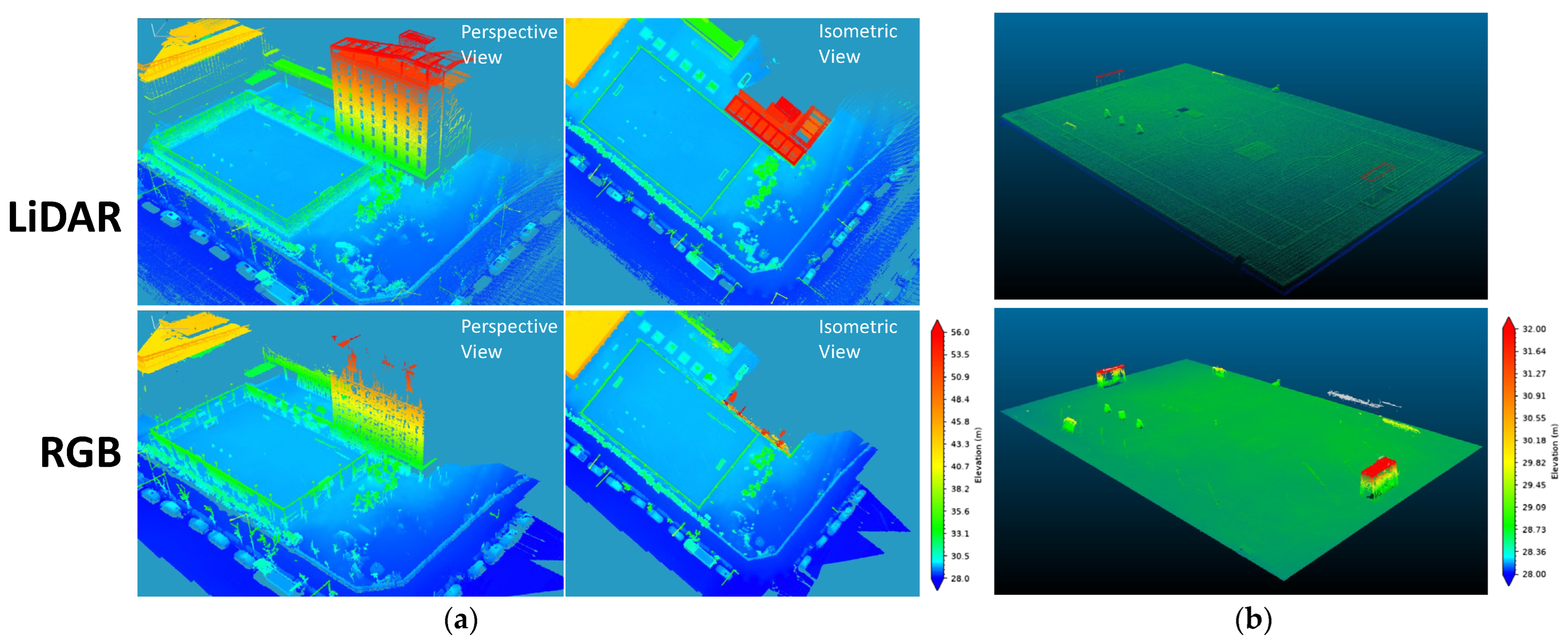
4.2. Quality and Vertical Accuracy of RGB and LiDAR Point Clouds

Figure 10a illustrates the point clouds generated from the LiDAR and RGB sensors. Figure 10b shows the enlarged point clouds of the playground. As seen in Figure 10, the RGB-driven point clouds showed good visual agreements with the LiDAR point clouds. The RGB point clouds were excessively denser than the LiDAR point clouds, but they had more artifacts and did not capture complex object characteristics. Specifically, the critical issue of the RGB point clouds was that the shadows on the ground had small elevations and some saturated uncertain points on the homogeneous surface, as seen in Figure 10b.

We statistically calculated the height of some objects on the ground.

Table 5. Comparisons of the object height between the LiDAR and RGB point clouds (unit: cm).

	Soccer Goals	Futsal Goals	A-Frame Signs
Ground Truth	210	120	85
LiDAR Height	211	122	86
RGB Height	205	118	87

summarizes the real and data-driven heights of the targets. The heights from the LiDAR point clouds were slightly more accurate than the RGB, but the differences between the two sensors were not significant. Although RGB-driven height information was acceptable, it was challenging to measure the generalized heights from the RGB point clouds due to significant artifacts and uncertainties, as seen in Figure 10, which must be handled by point cloud cleaning. Unlike photogrammetry, which uses multiple near-nadir images, LiDAR allows for the precise capturing of the building’s profile, including the architectural features, wall angles, and even small surface irregularities.

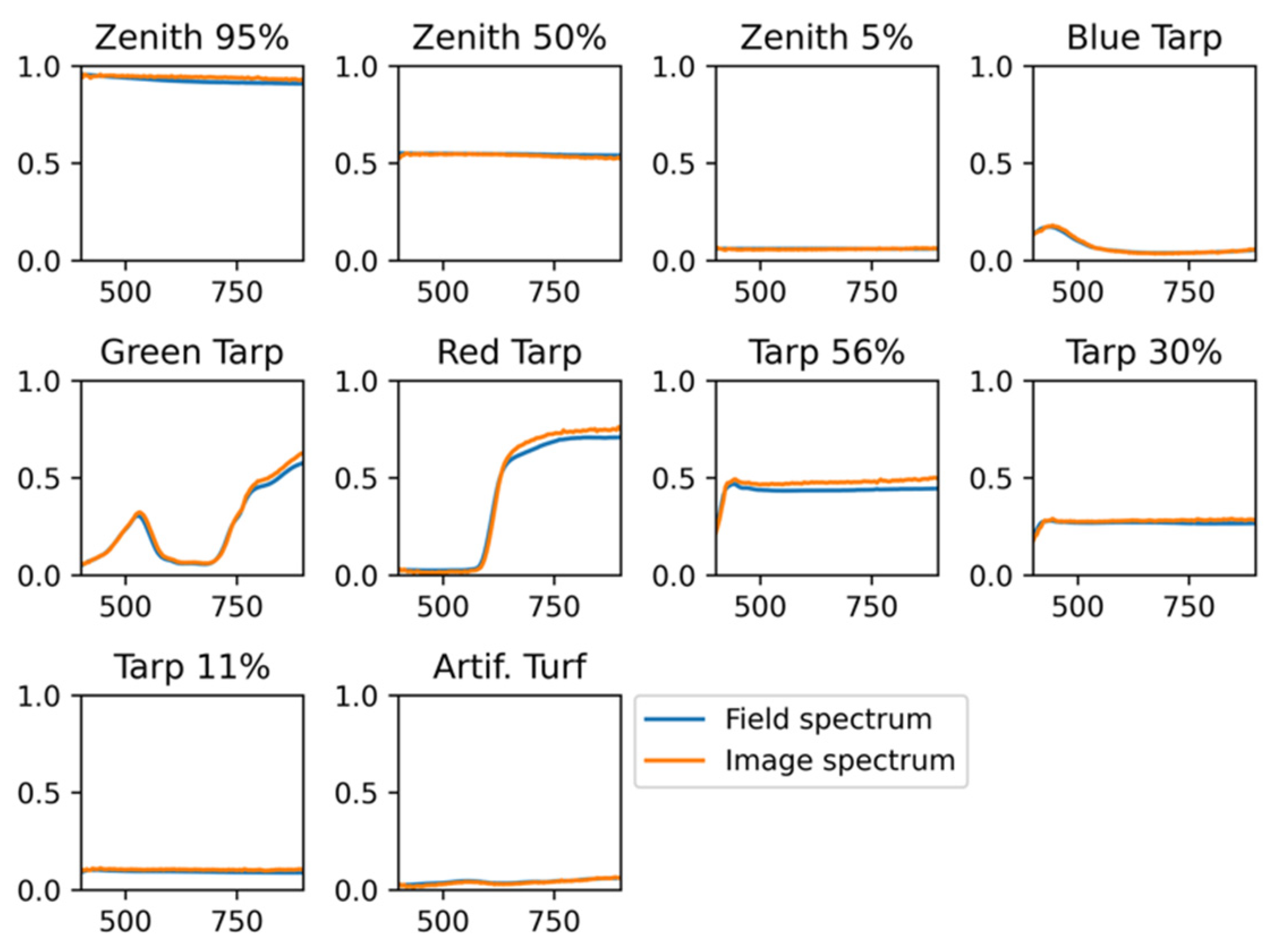
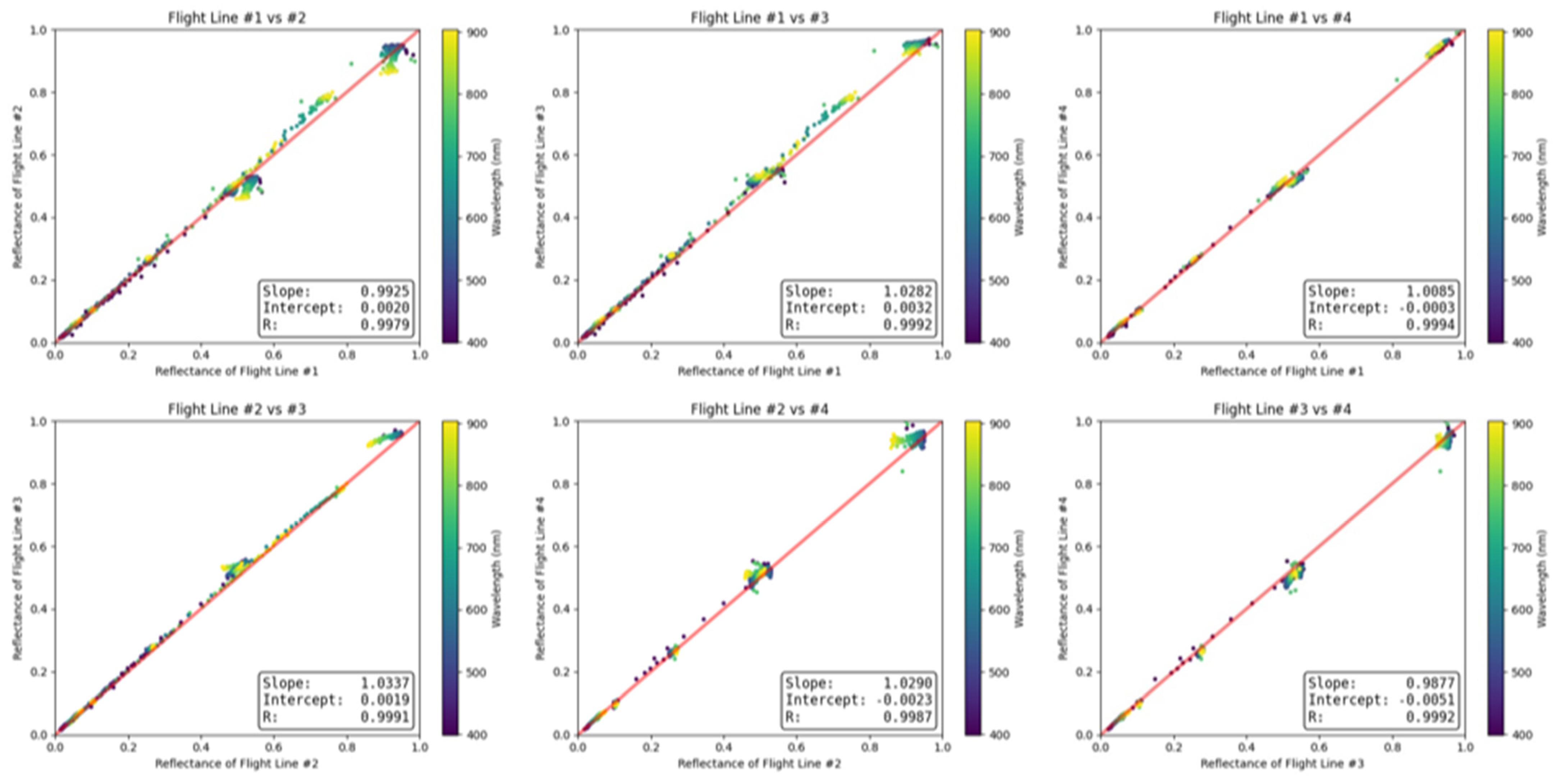
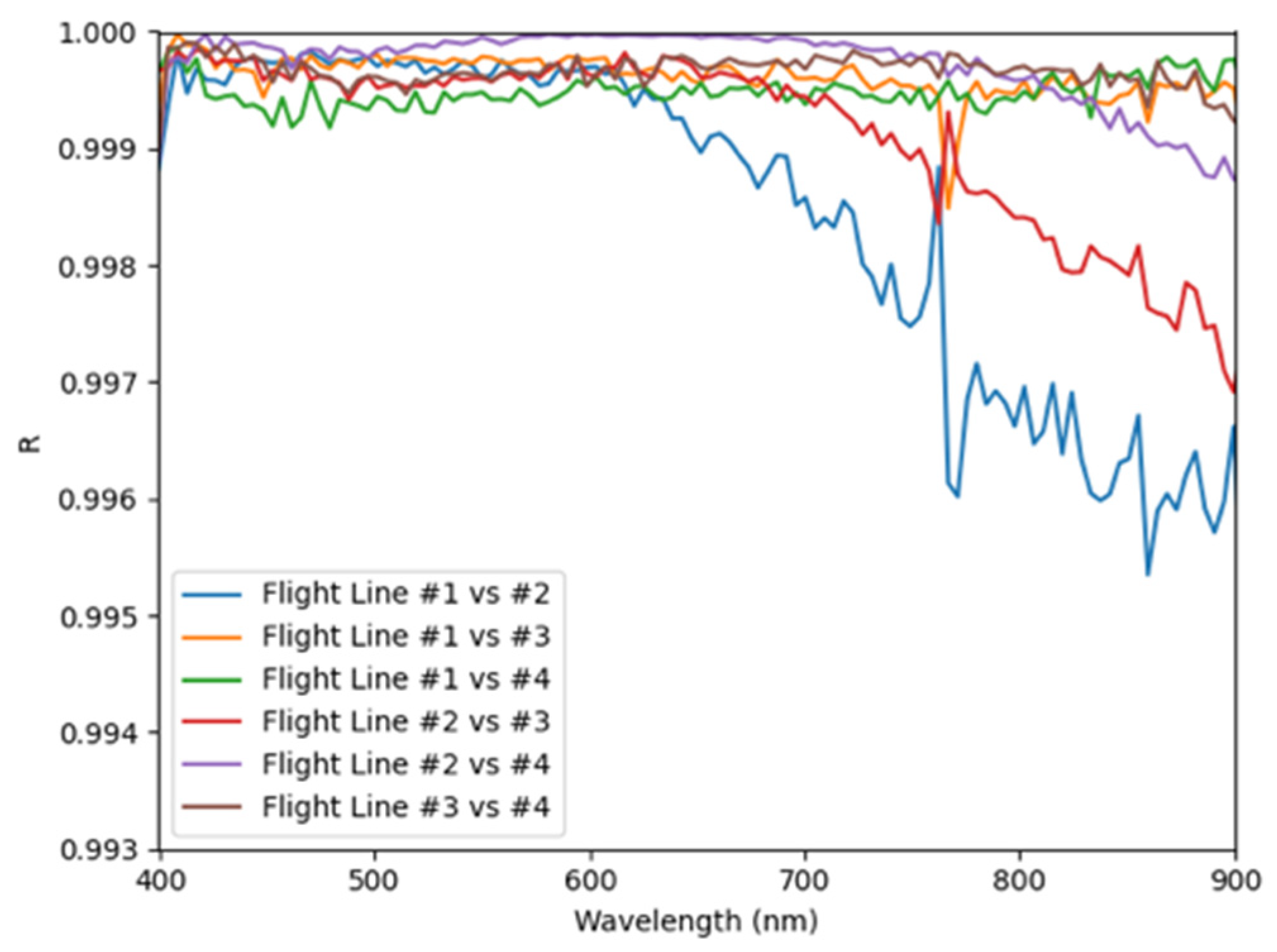
4.3. Radiometric Quality of Hyperspectral Images

Because we used the lab spectra of three zenith targets for the radiometric corrections, we compared the image-driven and field spectra to determine whether the in situ field spectra were required, as shown in Figure 11. The field spectra were averaged using ten iterative measurements for each target, and the image spectra were the mean spectral reflectance curves that were associated with the radiometrically corrected hyperspectral image pixels. We removed spectral bands that were above 900 nm because of the low signal-to-noise ratio. In Figure 11, the image spectra (orange lines) generally exhibit good visual agreement with the field spectra (blue lines). The absorption features and overall shapes of the target are preserved in the image spectra.

We compared the spectral angle and RMSE between the image-driven and field spectra for the quantitative analysis, as listed in

Table 6. Spectral angle and RMSE comparisons of the field and image spectra of the radiometric targets.

	Spectral Angle (Unit: Radian)	RMSE
Zenith 95%	0.0108	0.0194
Zenith 50%	0.0093	0.0080
Zenith 5%	0.0461	0.0031
Blue Tarp	0.0453	0.0041
Green Tarp	0.0333	0.0206
Red Tarp	0.0305	0.0312
56% Tarp	0.0281	0.0389
30% Tarp	0.0305	0.0129
11% Tarp	0.0360	0.0107
Artificial Turf	0.1031	0.0051

. Generally, a spectral angle that is less than 0.08 indicates a good similarity between two spectra, while a threshold for poor similarity is an angle that is greater than 0.14 [18]. All targets except for the artificial turf had a spectral angle of less than 0.05 with respect to the reference field spectrum. Although the spectral angle of the artificial turf was slightly larger than the cut-off for good similarity, it was fair. Compared with other targets, which were designed for radiometric correction, the surface of the artificial turf was not homogeneous. This may result in uncertainties in the field and image spectrum measurements. For the RMSE comparisons, all targets showed tiny differences in the brightness between the field and image spectra. The brightness temperature can vary according to the incidence angles and surface homogeneity. Therefore, the fabric targets showed relatively large RMSE values compared with the zenith targets, as the surface of the zenith targets is more homogeneous and similar to the Lambertian surface.

We acquired four overlapped images over the study area, as shown in Figure 2, and there were differences in the reflectance values for the same targets obtained from different flight trajectories due to the varying incidence angles. Figure 12 illustrates comparisons of the corresponding image reflectance values of the ground targets between different flight trajectories, with the wavelengths being denoted by the color intensity. The distribution of most match-up points in the scatter plots was formed around the one-to-one line with a near-zero offset. High Pearson correlation coefficients were achieved in all combinations. In Figure 13, we compared the Pearson correlation between the match-up reflectance values in terms of the wavelengths, showing high agreement. However, in these experiments, small differences were observed between the flight lines. Specifically, the correlation slightly decreased in longer wavelength ranges.

5. Discussions

UAV-borne geospatial data acquisitions have been recognized in various disciplines as they allow for more data to be recorded in less time. Integrating data from multiple sensors are more informative and provide the high capability of capturing various phenomena of the Earth’s surface. Although UAVs could supplement or even replace terrestrial survey methods for many applications, their accuracy has been called into question. The aim of this study was to answer three questions: (1) How accurate is direct georeferencing? Is a dedicated on-site base station required? (2) Do we need LiDAR sensors instead of RGB point clouds for vertical measurements? (3) Can hyperspectral data guarantee radiometric quality without incorporating a field spectrometer? To address these questions, we conducted experiments to compare the accuracy of the multi-sensor data acquired from an integrated UAV system with the ground truth.

Because the widely used GNSS/IMU for drones contains several meters of positioning errors [9], the installation and surveying of GCPs are required to guarantee reasonable geometric accuracy; however, it is costly and particularly ineffective for the pushbroom scanner, which requires EOPs for every scan line. However, the high-precision GNSS/IMU-assisted drone can produce sufficient quality to suggest this approach as a suitable alternative to a terrestrial survey. For the PPK of the GNSS/IMU data, the use of a dedicated on-site base station may be ideal, but one must pay for it, and it needs a piece of additional equipment to determine the accurate coordinates of the base station. Instead, we may want to use the CORSs that are located near the study area. Generally speaking, the geometric accuracy allows for roughly 1 cm of error per 10 km of distance to the base station [19,20]. However, our experiments demonstrated that there was no hard limit with respect to the baseline if a few centimeters of accuracy, which is equivalent to less than two hyperspectral pixels, is acceptable. While RTK technology uses broadcast ephemeris, which is transmitted from the navigation satellite in real time, PPK technology uses precision ephemeris, which provides precise satellite orbital information from International GNSS Service stations located around the world [21]. The reason for the low accuracy of the on-site base would be due to the inaccurate coordinates of the base station and number of visible satellites due to the relatively short mission time and 30 m tall building near the base station. Relatively high geometric errors of the JUNG station may be due to the atmospheric interference, which is one of the primary sources of GNSS receiver positioning error as well as orbital path error [22].

Overlapped, high-resolution RGB images could provide more dense point clouds than LiDAR and an acceptable vertical accuracy if the target points are reasonably selected. However, as photogrammetry relies on capturing multiple images from different viewpoints to extract 3D information, occlusions caused by objects or terrain features obstructing parts of the scene and shadows cast by objects can result in missing or inaccurate data, leading to errors in the DSM. As seen in our experimental results, the RGB point clouds included significant artifacts and unnecessary features and did not capture the detailed characteristics of the ground objects. For example, although we did not measure the heights of other objects, such as buildings, fences, trees, and cars around the soccer field, the LiDAR point clouds captured more details about the targets and had less noise than the RGB point clouds. This could be because LiDAR sensors emit laser pulses that directly penetrate and reflect off of the objects, while photogrammetry can be challenging due to the limited visibility from near-nadir angles. If necessary post-processing is applied to RGB point clouds, they can be utilized in the generation of DSMs for the orthorectification of relatively low-resolution images such as hyperspectral images; for the generation of a digital elevation (or terrain) model that ignores objects on the ground, however, photogrammetry will be problematic due to the occlusions and shadows compared with LiDAR’s laser signals. In addition, although we used very high-resolution RGB images to generate the point clouds, low-quality images, such as those affected by motion blur or noise, may lead to inaccurate elevation measurements. Image matching and tie-point selection algorithms that identify the corresponding features in multiple images are computationally expensive and challenging, especially in areas with repetitive patterns or textureless regions. Therefore, LiDAR technology should be highly recommended to extract accurate and detailed 3D information.

Finally, collecting the field spectra of radiometric targets during the mission may be ideal for the radiometric correction of hyperspectral data, but it requires additional cost. In our experiments, the use of lab spectra somewhat guarantees the radiometric quality regardless of the trajectories if there is no illumination change during the flight or contamination of the targets. The reasons for the small differences between the flight lines may be explained as follows: (1) there were different numbers in the overlapped pixels between the flight lines that needed to be calculated in the statistical comparisons; (2) there were slightly different pixel locations for the corresponding pixels between the flight lines though we performed accurate boresight calibrations; and (3) although we did not consider atmospheric attenuation because of the low flight altitude, decreasing atmospheric transmission in near-infrared may have resulted in relatively high errors in longer wavelengths [23].

References

1. Alex, T.; Maican, L.; Muhammad, H.B.M.H.; Joseph, G.D.; Jeannie, S.A.L.; Henrik, H.; Hoang, D.N. Drone-Based AI and 3D Reconstruction for Digital Twin Augmentation; Springer International Publishing: Berlin/Heidelberg, Germany, 2021; pp. 511–529. [Google Scholar]
2. Dong, J.; Zhuang, D.; Huang, Y.; Fu, J. Advances in Multi-Sensor Data Fusion: Algorithms and Applications. Sensors 2009, 9, 7771–7784. [Google Scholar] [CrossRef] [PubMed] [Green Version]
3. Sankey, T.; Donager, J.; McVay, J.; Sankey, J.B. UAV Lidar and Hyperspectral Fusion for Forest Monitoring in the Southwestern USA. Remote Sens. Environ. 2017, 195, 30–43. [Google Scholar] [CrossRef]
4. Goetz, A.F.H.; Vane, G.; Solomon, J.E.; Rock, B.N. Imaging Spectrometry for Earth Remote Sensing. Science 1985, 228, 1147–1153. [Google Scholar] [CrossRef] [PubMed]
5. Green, R.O.; Eastwood, M.L.; Sarture, C.M.; Chrien, T.G.; Aronsson, M.; Chippendale, B.J.; Faust, J.A.; Pavri, B.E.; Chovit, C.J.; Solis, M.; et al. Imaging Spectroscopy and the Airborne Visible/Infrared Imaging Spectrometer (AVIRIS). Remote Sens. Environ. 1998, 65, 227–248. [Google Scholar] [CrossRef]
6. Pearlman, J.S.; Barry, P.S.; Segal, C.C.; Shepanski, J.; Beiso, D.; Carman, S.L. Hyperion, a Space-Based Imaging Spectrometer. IEEE Trans. Geosci. Remote Sens. 2003, 41, 1160–1173. [Google Scholar] [CrossRef]
7. Loizzo, R.; Guarini, R.; Longo, F.; Scopa, T.; Formaro, R.; Facchinetti, C.; Varacalli, G. Prisma: The Italian Hyperspectral Mission. In Proceedings of the IGARSS 2018—2018 IEEE International Geoscience and Remote Sensing Symposium, Valencia, Spain, 22–27 July 2018; pp. 175–178. [Google Scholar] [CrossRef]
8. Adão, T.; Hruška, J.; Pádua, L.; Bessa, J.; Peres, E.; Morais, R.; Sousa, J. Hyperspectral Imaging: A Review on UAV-Based Sensors, Data Processing and Applications for Agriculture and Forestry. Remote Sens. 2017, 9, 1110. [Google Scholar] [CrossRef] [Green Version]
9. Sanz-Ablanedo, E.; Chandler, J.H.; Rodríguez-Pérez, J.R.; Ordóñez, C. Accuracy of Unmanned Aerial Vehicle (UAV) and SfM Photogrammetry Survey as a Function of the Number and Location of Ground Control Points Used. Remote Sens. 2018, 10, 1606. [Google Scholar] [CrossRef] [Green Version]
10. Martin, M.E.; Aber, J.D. High Spectral Resolution Remote Sensing of Forest Canopy Lignin, Nitrogen, and Ecosystem Processes. Ecol. Appl. 1997, 7, 431–443. [Google Scholar] [CrossRef]
11. Barreto, M.A.P.; Johansen, K.; Angel, Y.; McCabe, M.F. Radiometric Assessment of a UAV-Based Push-Broom Hyperspectral Camera. Sensors 2019, 19, 4699. [Google Scholar] [CrossRef] [PubMed] [Green Version]
12. Trimble APX-15 UAV Datasheet. Available online: https://www.applanix.com/downloads/products/specs/APX15_UAV.pdf (accessed on 17 March 2022).
13. Habib, A.; Zhou, T.; Masjedi, A.; Zhang, Z.; Flatt, J.E.; Crawford, M. Boresight Calibration of GNSS/INS-Assisted Push-Broom Hyperspectral Scanners on UAV Platforms. IEEE J. Sel. Top. Appl. Earth Obs. Remote Sens. 2017, 11, 1734–1749. [Google Scholar] [CrossRef]
14. Ravi, R.; Shamseldin, T.; Elbahnasawy, M.; Lin, Y.-J.; Habib, A. Bias Impact Analysis and Calibration of UAV-Based Mobile LiDAR System with Spinning Multi-Beam Laser Scanner. Appl. Sci. 2018, 8, 297. [Google Scholar] [CrossRef] [Green Version]
15. Kim, J.; Chi, J.; Masjedi, A.; Flatt, J.E.; Crawford, M.M.; Habib, A.F.; Lee, J.; Kim, H. High-resolution Hyperspectral Imagery from Pushbroom Scanners on Unmanned Aerial Systems. Geosci. Data J. 2022, 9, 221–234. [Google Scholar] [CrossRef]
16. Hruska, R.; Mitchell, J.; Anderson, M.; Glenn, N.F. Radiometric and Geometric Analysis of Hyperspectral Imagery Acquired from an Unmanned Aerial Vehicle. Remote Sens. 2012, 4, 2736–2752. [Google Scholar] [CrossRef] [Green Version]
17. Yuhas, R.H.; Goetz, A.F.; Boardman, J.W. Discrimination among Semi-Arid Landscape Endmembers Using the Spectral Angle Mapper (SAM) Algorithm. In Proceedings of the JPL, Summaries of the Third Annual JPL Airborne Geoscience Workshop, Pasadena, CA, USA, 1 January 1992; Volume 1, pp. 147–149. [Google Scholar]
18. L3 Harris Geospatial Documentation Center. Available online: https://www.l3harrisgeospatial.com/docs/thormaterialidentification.html (accessed on 7 April 2022).
19. Feng, Y.; Wang, J. GPS RTK Performance Characteristics and Analysis. J. Glob. Position. Syst. 2008, 7, 1–8. [Google Scholar] [CrossRef] [Green Version]
20. Khomsin; Anjasmara, I.M.; Pratomo, D.G.; Ristanto, W. Accuracy Analysis of GNSS (GPS, GLONASS and BEIDOU) Obsevation For Positioning. E3s Web Conf. 2019, 94, 01019. [Google Scholar] [CrossRef]
21. Ma, L.; Wang, X.; Li, S. Accuracy Analysis of GPS Broadcast Ephemeris in the 2036th GPS Week. IOP Conf. Ser. Mater. Sci. Eng. 2019, 631, 042013. [Google Scholar] [CrossRef]
22. Möller, G.; Landskron, D. Atmospheric Bending Effects in GNSS Tomography. Atmos. Meas. Tech. 2018, 12, 23–34. [Google Scholar] [CrossRef] [Green Version]
23. Kääb, A.; Bolch, T.; Casey, K.; Heid, T.; Kargel, J.S.; Leonard, G.J.; Paul, F.; Raup, B.H. Global Land Ice Measurements from Space. In Global Land Ice Measurements from Space; Springer: Berlin/Heidelberg, Germany, 2014; pp. 75–112. ISBN 9783540798170. [Google Scholar]
Figure 1. Integrated multi-sensor system onboard UAV.
Drones 07 00411 g001
Figure 2. Overview of the multi-sensor data acquisition. Targets for calibration and evaluation were deployed on the soccer field (red marks: ground control points; yellow rectangles: LiDAR targets; blue rectangles: radiometric targets).
Drones 07 00411 g002
Figure 3. Overview of the proposed study. The red, blue, and green rectangles are related to the geometric (X and Y directions) accuracy of orthomosaic images, vertical accuracy and qualitative quality of point clouds, and radiometric accuracy of the hyperspectral image, respectively.
Drones 07 00411 g003
Figure 4. Location of the base stations used in this study with the distance from the study area (KOPRI).
Drones 07 00411 g004
Figure 5. Example of histogram of target point clouds to determine the bottom/top height of the target.
Drones 07 00411 g005
Figure 6. Targets for radiometric correction and evaluation.
Drones 07 00411 g006
Figure 7. (a) DJI Phantom 4 image acquired on 21 February 2022; (b) DJI Phantom 4 image acquired on 22 February 2022; (c) RGB image acquired from the GNSS/IMU-assisted multi-sensor systems on 26 January 2022. Yellow lines are the geometric errors between the surveyed and image-driven coordinates.
Drones 07 00411 g007
Figure 8. Image locations of the surveyed GCPs in the hyperspectral orthomosaic image using the furthest CORS.
Drones 07 00411 g008
Figure 9. Illustrations of the positioning errors according to the distance of the CORS; The background image is a georeferenced orthomosaic generated from the RGB images of a frame camera for visual inspection.
Drones 07 00411 g009
Figure 10. Comparison of the LiDAR- and RGB-generated point clouds. (a) Overview of the study area; (b) enlarged point clouds.
Drones 07 00411 g010
Figure 11. Comparison of the field and image spectra of ten radiometric targets. Blue lines represent the field spectra of the targets, and orange lines are the mean spectral reflectance curves of the image pixels acquired using a hyperspectral sensor.
Drones 07 00411 g011
Figure 12. Comparison of the reflectance values for the same targets acquired from different flight trajectories.
Drones 07 00411 g012
Figure 13. Comparison of the correlation coefficients of the empirical line method according to the wavelengths.
Drones 07 00411 g013