Adjustable Fully Adaptive Cross-Entropy Algorithms for Task Assignment of Multi-UAVs

Abstract

This paper investigates the multiple unmanned aerial vehicle (multi-UAV) cooperative task assignment problem. Specifically, we assign different types of UAVs to accomplish the classification, attack, and verification tasks of targets under resource, precedence, and timing constraints. Due to complex coupling among these tasks, we decompose the considered problem into two subproblems: one with continuous and independent tasks and another with continuous and correlative tasks. To solve them, we first present an adjustable, fully adaptive cross-entropy (AFACE) algorithm based on the cross-entropy (CE) method, which serves as a stepping stone for developing other algorithms. Secondly, to overcome task precedence in the first subproblem, we propose a mutually independent AFACE (MIAFACE) algorithm, which converges faster than the CE method when obtaining the optimal scheme vectors of these continuous and independent tasks. Thirdly, to deal with task coupling in the second subproblem, we present a mutually correlative AFACE (MCAFACE) algorithm to find the optimal scheme vectors of these continuous and correlative tasks, while its computational complexity is inferior to that of the MIAFACE algorithm. Finally, numerical simulations demonstrate that the proposed MIAFACE (MCAFACE, respectively) algorithm consumes less time than the existing algorithms for the continuous and independent (correlative, respectively) task assignment problem.

1. Introduction

Due to its rapid deployment and nearly unlimited mobility, an unmanned aerial vehicle (UAV) has great potential in both military and civilian applications, including modern warfare, disaster search and rescue, traffic control, celestial exploration, and a variety of other fields [1,2,3,4]. UAVs for these applications have limited capabilities and require sufficient resources to perform tasks autonomously. As a result, multi-UAVs can be regarded as a promising method by which to handle complex tasks. As more attention is focused on them, two problems in multi-UAV collaboration, such as multi-UAV cooperative path planning and cooperative task assignment, are becoming more widely recognized. The main consideration of this paper is the multi-UAV cooperative task assignment problem.

In recent years, many scholars have paid attention to the multi-UAV cooperative task assignment problem, while the related research of this problem is as follows. Chen et al. [5] utilized mixed integer linear programming (MILP) to address the problem of multi-UAV cooperative task assignment and path planning for moving targets on the ground, but it had low scalability while maintaining global optimality. References [6,7] used a heuristic approach to produce near-optimal results in real time, which has been widely considered for large-scale problems and dynamic scenarios. For swarm intelligence algorithms, e.g., particle swarm optimization (PSO) [8], ant colony optimization (ACO) [9], and genetic algorithm (GA) [10], when solving the task assignment problem, they had a fast convergence speed and could effectively obtain optimal assignment schemes, but there is a possibility of falling into local optimum. Moreover, the auction algorithm, game theory, and reinforcement learning have also been applied to the multi-UAV task assignment problem. Duan et al. [11] presented a novel hybrid “two-stage” auction algorithm that combines the structural advantages of the centralized and distributed auction algorithms, which greatly facilitates the performance of UAVs in dynamic task assignments. Chen et al. [12] studied the cooperative reconnaissance and spectrum access (CRSA) problem for task-driven heterogeneous coalition-based UAV networks, and proposed a joint bandwidth allocation and coalition formation (JBACF) algorithm to solve the task assignment and bandwidth allocation. Qie et al. [13] proposed an artificial intelligence method called simultaneous target assignment and path planning (STAPP) to solve the multi-UAV target assignment and path planning problem, and the effectiveness of the algorithm was experimentally verified. In addition, references [14,15,16,17,18,19,20,21] provide a variety of alternative algorithms for the solution of analogous problems.

Similarly, some novel works on task assignment, e.g., UAV-assisted task assignment, have been presented. Liu et al. [22] studied a UAV-assisted IoT system while presenting a nonconvex age-of-information (AoI) minimization problem, which was solved by jointly optimizing task assignment, interaction point selection (IPT), and UAV trajectories. Zhu et al. [23] considered the problem of task loss rate (TLR) fairness among IoTs and equal energy consumption (EC) fairness among UAVs, and proposed a multiagent deep deterministic policy gradient (MA-DDPG) method by which to assign UAVs to accomplish tasks and guarantee the balance between IoT TLR and UAV EC. Seid et al. [24] considered the assignment of UAVs to perform aerial base station tasks based on a multi-UAV-assisted IoT network framework, while presenting a joint optimization problem for computational offloading with energy harvesting (EH) and resource price, and the resource demands and pricing strategies between IoT devices and UAVs were continuously adjusted by the Stackelberg game. Hu et al. [25] considered the aging of cache refreshing, computation offloading, and state updates in UAV-assisted vehicle task awareness, and formulated a task-assignment energy-minimization problem that was solved by a deep deterministic policy gradient (DDPG) method. Zhou et al. [26] studied UAV-assisted mobile crowd sensing (MCS) scenarios and proposed a UAV-assisted multitasking assignment (UMA) method, while demonstrating the effectiveness of UMA. In addition, compared the UAV-assisted task assignment with the UAV task assignment, the difference is that UAVs play a secondary role in the former while serving as the primary reconnaissance and attack objects in the latter. Furthermore, the simulation scenarios in the paper are not consistent with the existing works (e.g., references [22,23,24,25,26]).

In the complex stochastic network, the cross-entropy (CE) method [27], a relatively new technique for dealing with combinatorial optimization problems, was initially utilized to estimate rare event probabilities. Then, references [28,29] discussed and analysed its convergence. Additionally, the cross-entropy (CE) method was proved by the authors in [30] to be particularly meaningful for handling combinatorial optimization problems. Since then, it has also been proven by many scholars to be a simple and effective tool for different fields, e.g., vehicle routing [31], buffer allocation [31], and machine learning [32]. In addition, researchers have also considered applying the cross-entropy (CE) method to the UAV task assignment [33,34,35]. However, the authors of these papers did not consider the specific precedence and timing constraints among these tasks.

When it comes to task-assignment schemes in the field of UAVs, some researchers usually assume that each UAV is assigned to only one target, and they rarely consider the execution sequence and the time constraints among tasks. On the other hand, multi-UAVs are sometimes needed to perform some complex combinatorial tasks, such as classifying the target, attacking it, and then verifying the target’s damage level in a reasonable time on the battlefield. In addition, such deterministic approaches may not be able to find the optimal solution in a reasonable time for large-scale task assignment problems. Under these circumstances, we present an adjustable fully adaptive cross-entropy (AFACE) algorithm based on CE method.

Therefore, the purpose of this paper is to study the AFACE algorithm for the multi-UAV cooperative task assignment problem under resource, precedence, and timing constraints. The main contributions are summed up as follows.

• We consider the multi-UAV cooperative task assignment problem in which different types of UAVs are assigned to perform classification, attack and verification tasks of targets under resource, and precedence and timing constraints. Considering complex coupling among these tasks, we decompose the considered problem into two subproblems: one with continuous and independent tasks and another with continuous and correlative tasks.
• We propose an AFACE algorithm, which changes the random sample and the quantile at each iteration and adds a parameter to adjust the maximum sample based on the CE method. Meanwhile, the algorithm serves as a stepping stone for developing other algorithms.
• To overcome task precedence and task coupling existing in these two problems, respectively, we present a mutually independent AFACE (MIAFACE) algorithm and a mutually correlative AFACE (MCAFACE) algorithm with polynomial time complexity. The former algorithm converges faster than the CE method, while the computational complexity of the latter algorithm is inferior to that of the former algorithm.
• Simulation results demonstrate that both MIAFACE and MCAFACE algorithms consume less time than other existing optimization algorithms for solving the corresponding problem.

The rest of this paper is organized as follows. In Section 2, we introduce the related works of the CE method and other algorithms for the UAV task assignment. Section 3 depicts the multi-UAV cooperative task assignment problem with its mathematical formulation. In Section 4, we decompose the considered problem into two subproblems, and propose an AFACE algorithm, a MIAFACE algorithm, and a MCAFACE algorithm, and apply the latter two algorithms to solving the corresponding problem. Section 5 conducts several simulations and comparisons to verify the feasibility and effectiveness of the proposed algorithms. This paper is concluded in Section 6.

2. Related Work

This section reviews the related works on CE method and other algorithms used for UAV task assignment.

2.1. CE Method Used for UAV Task Assignment

Due to CE’s merits, the authors of [33] first proposed using the CE method for tackling the multi-UAV task assignment problem to tackle the large traveling salesman problem (TSP), the vehicle routing problem (VRP), and Markov decision process (MDP). In particular, compared to other algorithms, CE could solve optimization problems efficiently because of its ability to deal with these problems with nonlinear objective functions. Three separate multi-UAV task assignment problems were then formulated, including a nonlinear objective function with distance penalty, a nonlinear objective function with no distance penalty, and nonlinear constraints. In these problems, the authors considered the distance penalty and required that each task must be assigned to at least one vehicle. Then, the task scores were considered as nonlinear functions, and the CE method was used to determine the optimal schemes for the functions of these problems. Finally, simulation results verified that the performance of the CE method was superior to other algorithms.

The authors in [34] considered the multi-UAV task assignment problem. Then, the score function of this problem was determined with the constraint that each UAV was used for only one task. Subsequently, the CE method was used to find the optimal scheme of this problem. Finally, simulation results showed that the CE method outperformed the Branch and Bound algorithm in solving the above problem, especially on a large scale.

Referring to [33,34], the authors in [35] described the multitype UAV task assignment problem. In this problem, different types of UAVs, or the same type of UAV as well as resource constraints, were considered. The authors then formulated the problem and provided a score function under resource constraints. Then, the CE method was used to determine the optimal scheme of this problem by assigning multitype UAVs to complete tasks. Finally, numerical simulations of the CE method for task assignment, as well as comparisons with the exhaust search method, were conducted to verify its merits in solving the considered problem.

In [36], the authors first analyzed the CE method, then redefined its construct and applied it to UAV swarms. Subsequently, due to the robustness of this method, it could be used as an effective measure to control UAV swarms in the face of obstacles and unforeseen problems. Finally, it was validated to support UAV swarms in achieving mission objectives.

The authors of [37] considered the multi-UAV task assignment problem under resource constraint and precedence constraint. The fully adaptive cross-entropy (FACE) algorithm based on the CE method was then applied to solve the considered problem. Then, simulation results verified that the FACE algorithm was better than the CE method and PSO algorithm in terms of convergence speed.

2.2. Other Algorithms Used for UAV Task Assignment

The authors in [8] improved the PSO algorithm with an inertia weight factor and applied it to handle the multi-UAV task assignment problem, then conducted several simulations and comparisons. Then, it was verified that the improved algorithm has a faster convergence speed and global optimization capability compared with the standard PSO algorithm.

In [38], the authors presented a novel hierarchical task assignment method to solve the multi-UAV task assignment problem, and the method was decomposed into two phases, including the hierarchical decomposition phase and the task assignment phase. The former phase reduced the computational complexity by using the balance cluster method to simplify the large-scale UAV model; the latter phase maintained the diversity of the population by an improved firefly algorithm. Then, simulations showed that compared with other algorithms, the proposed hierarchical method becomes more efficient in terms of search ability and convergence speed.

The authors in [39] defined the task assignment problem for cooperative multi-UAV road network reconnaissance and formulated a multi-UAV road network reconnaissance traveling salesman problem (MRRTSP) model. Furthermore, a customized genetic algorithm for road network reconnaissance (CGA-RNR) was proposed and used to solve the considered problem. Then, simulations showed that the algorithm can quickly obtain feasible solutions and converge to the optimal solution.

3. Problem Description and Formulation

The main parameters of this paper is shown in Table 1.

Table 1. Simulation parameter settings.

Variables	Explanation
$N_{\mathrm{b}}$	The number of bases
$N_{\mathrm{t}}$	The number of targets
j	The target index
$\mathcal{K}$	The set of tasks of targets
$N_{\mathrm{m}}$	The number of tasks of targets
m	The task index of targets
$\mathcal{X}$	The set of all possible UAV deployment schemes
L	The number of $\mathcal{X}$ for each task
z	The maximum number of UAVs in each scheme of $\mathcal{X}$
$\mathcal{Z}$	The set of all possible UAV deployment scheme indexes
k	A UAV deployment scheme index or a UAV formation index
$\mathit{x}(m)$	A feasible UAV deployment scheme vector of task m
$x_j(m)$	A feasible UAV deployment scheme or a UAV formation of task m of target j
$g(x_j(m);k)$	A 0–1 decision variable
$\mathcal{Y}$	The set of all feasible $\mathit{x}(m)$
$\Omega (\mathit{x}(m))$	The performance of task m
$\Omega$	The performance vector of $\Omega (\mathit{x}(m))$
$\rho$	The total objective function
$\psi (x_j(2))$	The reward benefit of the attack task of target j
$\phi (x_j(m))$	The cost of assigning UAV formation $x_j(m)$ to accomplish task m of target j
$p_{\mathrm{k}}^j$	The probability of killing target j
$p_{\mathrm{s}}^j$	The UAV survival probability of accomplishing tasks of target j
$w_1$, $w_2$ and $w_3$	Weight coefficients
$P_{\mathrm{c}}$ and V	The target identification certainty and the constant velocity of each UAV
$y_j$ and $s_j$	The value and the threat level of target j
$d_j(m)$	The farthest distance from the base corresponding to UAV formation $x_j(m)$ to target j
$D_{\max }$	The maximum flying distance
$T_m$	The execution time of task m

Problem Description

On the battlefield, multi-UAVs are deployed to perform different tasks, for example, to classify targets before attacking them, and then to verify them to check whether these tasks have been accomplished. The problem considered in this paper is the selection of a mix of the same type of UAV or different types of UAVs from their bases to perform the classification, attack and verification tasks of targets. As shown in Figure 1, there are $N_{\mathrm{b}}$ types of UAVs with the same speed, and the related components of this problem can be defined as a 5-tuple $\{\mathcal{A},\mathcal{B},\mathcal{G},\mathcal{K},\mathcal{T}\}$. In the 5-tuple, $\mathcal{A}:=\{1,2,\dots ,N_{\mathrm{m}}\}$ denotes the set of task index of targets, $\mathcal{B}:=\{1,2,\dots ,N_{\mathrm{b}}\}$ represents the set of $N_{\mathrm{b}}$ bases, $\mathcal{G}:=\{1,2,\dots ,N_{\mathrm{t}}\}$ denotes the set of $N_{\mathrm{t}}$ targets with known positions, $\mathcal{K}:=\{K_1,K_2,\dots ,K_{N_{\mathrm{m}}}\}$ represents the set of $N_{\mathrm{m}}$ tasks of targets, and $\mathcal{T}:=\{T_1,T_2,\dots ,T_{N_{\mathrm{m}}}\}$ denotes the set of the execution time of $N_{\mathrm{m}}$ tasks of targets. Note that the time required to allocate tasks is ignored.

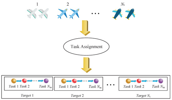
Figure 1. Task assignment diagram.

Moreover, let $\mathit{x}(m)={[x_1(m),x_2(m),\dots ,x_{N_{\mathrm{t}}}(m)]}^T$ denote a feasible UAV deployment scheme vector, and define $\mathcal{Y}$ as the set of all feasible $\mathit{x}(m)$. Let $\mathcal{Z}:=\{1,2,\dots ,L\}$ be the set of all possible UAV deployment scheme indices. Thus, $\mathit{x}(m)$ satisfies

$$g(x_j(m);k)=\left\{\begin{array}{c}1,if\varphi (x_j(m))=k,j\in \mathcal{G},m\in \mathcal{A},k\in \mathcal{Z}\hfill \\ 0,if\varphi (x_j(m))\ne k,x_j(m)\in \mathcal{X}\hfill \end{array}\right.,$$

(1)

where j denotes the target index, m designates the task index, $x_j(m)$ is a feasible UAV deployment scheme or a UAV formation of task m of target j, k represents a UAV deployment scheme index or a UAV formation index, $\varphi (x_j(m))$ is an index function that serves to output the subscript corresponding to $x_j(m)$ in $\mathcal{X}$, and $g(x_j(m);k)$ is a 0–1 decision variable, i.e., the kth UAV formation is assigned to accomplish task m of target j.

Then, the total objective function $\rho$ based on $\mathit{x}(m)$ is defined as

$$\begin{array}{cc}\hfill \rho & ={\displaystyle \sum _{m=1}^{N_{\mathrm{m}}}}\Omega (\mathit{x}(m))\hfill \\ \hfill & ={\displaystyle \sum _{j=1}^{N_t}}\psi (x_j(2))-{\displaystyle \sum _{m=1}^{N_{\mathrm{m}}}}{\displaystyle \sum _{j=1}^{N_{\mathrm{t}}}}\phi (x_j(m)),\hfill \end{array}$$

(2)

where $\Omega (\mathit{x}(m))$ is the subobjective function of task m, $\psi (x_j(2))$ and $\phi (x_j(m))$ denote the reward benefit of the attack task and the cost of assigning $x_j(m)$ to accomplish tasks of target j, respectively, which are

$$\begin{array}{cc}\hfill \psi (x_j(2))& =w_1\times P_{\mathrm{c}}\times p_{\mathrm{k}}^j\times y_j\hfill \end{array}$$

(3)

$$\begin{array}{cc}\hfill \phi (x_j(m))& =w_2\times p_{\mathrm{s}}^j\times s_j+w_3\times (V\times T_m+d_j(m)),\hfill \end{array}$$

(4)

where $P_{\mathrm{c}}$ is the target identification certainty, $y_j$ represents the value of target j, $s_j$ denotes the threat level of target j, V is the constant velocity of each UAV, $T_m$ represents the execution time of task m, $d_j(m)$ denotes the farthest distance from the bases corresponding to UAV formation $x_j(m)$ to target j, $w_1$, $w_2$ and $w_3$ represent weight coefficients, indicating the information about the relative importance of each subobjective, $p_{\mathrm{k}}^j$ denotes the probability of killing target j, and $p_{\mathrm{s}}^j$ is the UAV survival probability of accomplishing task m of target j.

In addition, $p_{\mathrm{k}}^j$ and $p_{\mathrm{s}}^j$ are defined as

$$\begin{array}{cc}\hfill p_{\mathrm{k}}^j& =\prod _{a\in x_j(2)}{p}_{aj}\hfill \end{array}$$

(5)

$$\begin{array}{cc}\hfill p_{\mathrm{s}}^j& =1-\prod _{b\in x_j(m)}{p}_{bj},\hfill \end{array}$$

(6)

where a stands for a UAV in UAV formation $x_j(2)$; $p_{aj}$ is the probability of killing target j with UAV a, b represents a UAV in UAV formation $x_j(m)$, and $p_{bj}$ is the UAV survival probability of accomplishing task m of target j with UAV b.

According to Equations (2)–(6), $\rho$ is rewritten as

$$\begin{array}{cc}\hfill \rho =& {\displaystyle \sum _{j=1}^{N_{\mathrm{t}}}}{w}_1\times P_{\mathrm{c}}\times p_{\mathrm{k}}^j\times y_j-{\displaystyle \sum _{m=1}^{N_{\mathrm{m}}}}{\displaystyle \sum _{j=1}^{N_{\mathrm{t}}}}[w_2\times p_{\mathrm{s}}^j\times s_j\hfill \\ \hfill & +w_3\times (V\times T_m+d_j(m))].\hfill \end{array}$$

(7)

Then, our objective is to maximize $\rho$, and the considered problem can be formulated as

$$\begin{array}{cc}\hfill \mathcal{P}:\underset{\mathit{x}(m)\in \mathcal{Y}}{max}& \rho ={\displaystyle \sum _{m=1}^{N_{\mathrm{m}}}}\Omega (\mathit{x}(m))\hfill \end{array}$$

(8)

$$\begin{array}{cc}\hfill \mathrm{s}.\mathrm{t}.& w_1+w_2+w_3=1,0\le w_1,w_2,w_3\le 1\hfill \end{array}$$

(9)

$$\begin{array}{cc}\hfill & d_j(m)+V\times T_m\le D_{\max }\forall j,m\hfill \end{array}$$

(10)

$$\begin{array}{cc}\hfill & K_1^j\prec K_2^j\prec K_3^j\forall j.\hfill \end{array}$$

(11)

Constraint (9) represents the range of $w_1$, $w_2$, and $w_3$. Constraint (10) is that, for target j, the sum of $d_j(m)$ and the farthest flying distance performed by the UAV formation $x_j(m)$ does not exceed the maximum flying distance $D_{\max }$. Constraint (11) means that $K_1^j$, $K_2^j$, and $K_3^j$ are the classification, attack, and verification tasks of the target j, which are executed in a specific order, and ≺ denotes the preceding symbol.

According to Equation (11), the specific precedence and timing constraints are equal to

$$\left\{\begin{array}{c}{t}_{\mathrm{s}1}^j\ge {\mathrm{s}}_1,{\mathrm{e}}_1\ge t_{\mathrm{s}1}^j+T_1\hfill \\ t_{\mathrm{s}2}^j\ge {\mathrm{s}}_2,{\mathrm{e}}_2\ge t_{\mathrm{s}2}^j+T_2\hfill \\ t_{\mathrm{s}3}^j\ge {\mathrm{s}}_3,{\mathrm{e}}_3\ge t_{\mathrm{s}3}^j+T_3\hfill \end{array}\right.,$$

(12)

where $[{\mathrm{s}}_1,{\mathrm{e}}_1]$, $[{\mathrm{s}}_2,{\mathrm{e}}_2]$, and $[{\mathrm{s}}_3,{\mathrm{e}}_3]$ represent the classification, attack, and verification time windows and $t_{\mathrm{s}1}^j$, $t_{\mathrm{s}2}^j$ and $t_{\mathrm{s}3}^j$ denote the start time of classification, attack, and verification tasks of the target j, respectively.

Moreover, we set a certain value $\gamma$, which ensures that the optimal scheme vector ${\mathit{x}}^{*}(m)$ conforms to $\Omega ({\mathit{x}}^{*}(m))\ge \gamma$. After that, the maximum ${\rho }^{*}$ is written as

$${\rho }^{*}={\displaystyle \sum _{m=1}^{N_{\mathrm{m}}}}\Omega ({\mathit{x}}^{*}(m))\ge N_{\mathrm{m}}\gamma .$$

(13)

Therefore, to obtain ${\mathit{x}}^{*}(m)$, we present an AFACE algorithm.

4. Algorithm Analysis

In this section, an AFACE algorithm will be introduced for the considered problem, and the differences between the algorithm and cross-entropy (CE) method are that the former changes the random sample $N_{\mathrm{d}}^t$ and the quantile ${\theta }_t$ at each iteration t, and adds a parameter to adjust the maximum sample $N^{\max }$. For details, please refer to the analysis of the algorithm below.

4.1. Adjustable Fully Adaptive Cross-Entropy Algorithm

Referring to the principle of CE method in references [30,35] and maximizing the subobjective function $\Omega (\mathit{x}(m))$ of the considered problem, we have

$${\gamma }^{*}=\Omega ({\mathit{x}}^{*}(m))=\underset{\mathit{x}(m)\in \mathcal{Y}}{max}\Omega (\mathit{x}(m)),$$

(14)

where ${\gamma }^{*}$ is the maximum of $\Omega (\mathit{x}(m))$ on $\mathcal{Y}$; that is, the optimal scheme vector is ${\mathit{x}}^{*}(m)$.

After that, transform this problem into a probability estimator problem, which can be explained by the probability density function (PDF) $f(·;u)$ with respect to u, and the problem can be written as

$$\begin{array}{cc}\hfill \ell (\gamma )& ={\mathbb{P}}_u(\Omega (\mathit{x}(m))\ge \gamma )\hfill \\ \hfill & =\sum _{\mathit{x}(m)}{I}_{\{\Omega (\mathit{x}(m))\ge \gamma \}}f(\mathit{x}(m);u)\hfill \\ \hfill & ={\mathbb{E}}_u{I}_{\{\Omega (\mathit{x}(m))\ge \gamma \}},\hfill \end{array}$$

(15)

where $\gamma$ denotes a value close to ${\gamma }^{*}$, ${\mathbb{P}}_u$ represents the probability measure under which the random vector $\mathit{x}(m)$ has the PDF $f(·;u)$, ${\mathbb{E}}_u$ is the corresponding expectation operator, and $I(\mathit{x}(m);\gamma )$, i.e., $I_{\{\Omega (\mathit{x}(m))\ge \gamma \}}$, denotes the indicator function, which is

$$I(·;\gamma )=\left\{\begin{array}{c}1,if\Omega (\mathit{x}(m))\ge \gamma \hfill \\ 0,if\Omega (\mathit{x}(m))<\gamma \hfill \end{array}\right..$$

(16)

Then, at the tth iteration of AFACE algorithm, we obtain

$${\Omega }_{t,1}\le \cdots {\Omega }_{t,i}\le \cdots \le {\Omega }_{t,N_{\mathrm{d}}^t},$$

(17)

where ${\Omega }_{t,i}$ ($i=1,2,\dots ,N_{\mathrm{d}}^t$) denotes the ith sample performance, and $\Omega ({\mathit{x}}_i(m)))$ and ${\Omega }_{t,N_{\mathrm{d}}^t}$ are defined by ${\Omega }_{t,i}$ and ${\Omega }_t^{*}$ for convenience. Meanwhile, AFACE algorithm parameters $N_{\mathrm{d}}^t$ and ${\theta }_t$ satisfy

$$\left\{\begin{array}{c}{N}^{\min }\le N_{\mathrm{d}}^t\le N^{\max }\hfill \\ {\theta }_t={\beta }_m/N_{\mathrm{d}}^t\hfill \end{array}\right.,$$

(18)

where $N_{\mathrm{d}}^t$ denotes the random sample of the tth iteration, varying between $N^{\min }$ and $N^{\max }$ ($N^{\min }=N,N^{\max }=hN,h\in \{2,3,4,5\}$) and ${\theta }_t$ represents the quantile of the tth iteration. The reason for presenting h is that by adjusting the size of $N^{\max }$, we can obtain the optimal $N^{\max }$ that matches the combat scenario, which can be conducted by the following simulations in Section 5.

For the AFACE algorithm, the main idea is to update $N_{\mathrm{d}}^t$ and ${\theta }_t$ based on the elite sample ${\beta }_m$ (${\beta }_m=c_{m}N$), where $c_m$ and N are the elite sample influence coefficient of task m (usually $0.01\le c_m\le 0.1$) and the fixed random sample, respectively. Therefore, the set of elite samples ${\epsilon }_t$ (${\epsilon }_t\in \mathcal{Y}$) are comprised of such ${\beta }_m$ samples in $\{{\mathit{x}}_1(m),{\mathit{x}}_2(m),\dots ,{\mathit{x}}_{N_{\mathrm{d}}^t}(m)\}$ with the highest performances ${\Omega }_{t,1},{\Omega }_{t,2},\dots ,{\Omega }_{t,N_{\mathrm{d}}^t}$.

Next, referring to the formulas for solving ${\widehat{\gamma }}_t$ and ${\widehat{v}}_t$ of CE method [30], they are modified as

$$\begin{array}{cc}\hfill {\widehat{\gamma }}_t& ={\Omega }_{(\lceil (1-{\theta }_t)N_{\mathrm{d}}^t\rceil )}\hfill \end{array}$$

(19)

$$\begin{array}{cc}\hfill {\widehat{v}}_t& =\underset{v}{argmax}\sum _{{\mathit{x}}_i(m)\in {\epsilon }_t}lnf({\mathit{x}}_i(m);v),\hfill \end{array}$$

(20)

where ${\mathit{x}}_i(m)$ is generated from $f(·;u)$, $f(·;v)$ denotes another PDF with respect to v on $\mathcal{Y}$ via minimizing the Kullback–Leibler distance, ${\widehat{\gamma }}_t$ is equal to the worst sample performance among the elite performances, while ${\Omega }_t^{*}$ is the best sample performance among the elite performances, and ${\widehat{v}}_t$ converges to the probability density when ${\Omega }_t^{*}$ occurs.

Then, we devise a sampling scheme for each iteration t, ensuring high probability that

$$\left\{\begin{array}{c}{\Omega }_t^{*}>{\Omega }_{t-1}^{*}\hfill \\ {\widehat{\gamma }}_t>{\widehat{\gamma }}_{t-1}\hfill \end{array}\right..$$

(21)

Moreover, we simultaneously generate two sequences to validate the correctness of AFACE algorithm. One is the levels ${\widehat{\gamma }}_1,{\widehat{\gamma }}_2,\dots ,{\widehat{\gamma }}_t$, and the other is the parameters ${\widehat{v}}_1,{\widehat{v}}_2,\dots ,{\widehat{v}}_t$. After that, the initialization process is set to ${\widehat{v}}_0=u$, and the quantile ($1-{\theta }_t$) is calculated at the tth iteration according to Equation (18), followed by the next two steps of Algorithm 1.

In addition, the main steps of AFACE algorithm applied to solving the subobjective function $\Omega (\mathit{x}(m))$ of the considered problem are given by Algorithm 2.

Algorithm 1 Adaptive updating of ${\widehat{\gamma }}_t$ and ${\widehat{v}}_t$.

Adaptive updating of ${\widehat{\gamma }}_t$: 1: Given a fixed ${\widehat{v}}_{t-1}$ at the tth iteration; 2: Let ${\gamma }_t$ be a ($1-{\theta }_t$)-quantile of $\Omega (\mathit{x}(m))$ under ${\widehat{v}}_{t-1}$, then ${\gamma }_t$ satisfies ${\mathbb{P}}_{{\widehat{v}}_{t-1}}(\Omega (\mathit{x}(m))\le {\gamma }_t)\ge 1-{\theta }_t$, where $\mathit{x}(m)\sim f\left(·;{\widehat{v}}_{t-1}\right)$; 3: Obtain a simple estimator ${\widehat{\gamma }}_t$ of ${\gamma }_t$ by drawing $N_{\mathrm{d}}^t$ random samples ${\mathit{x}}_1(m),{\mathit{x}}_2(m),\dots ,{\mathit{x}}_{N_{\mathrm{d}}^t}(m)$ from $f(·;{\widehat{v}}_{t-1})$; 4: Calculate and order all performances of $\Omega (\mathit{x}(m))$ from smallest to biggest: ${\Omega }_{t,1}\le \cdots \le {\Omega }_{t,N_{\mathrm{d}}^t}$; 5: Compute ${\widehat{\gamma }}_t$ according to Equation (19); Adaptive updating of ${\widehat{v}}_t$: 6: Given a fixed ${\widehat{\gamma }}_t$ and ${\widehat{v}}_{t-1}$ at the tth iteration, then derive ${\widehat{v}}_t$ according to Equation (20).

Algorithm 2 AFACE algorithm.

Input: ${\widehat{v}}_0$, h, N. Output: ${\Omega }_t^{*}$. 1: Set t = 1, $N^{\min }=N$ and $N^{\max }=hN$; 2: while at the tth iteration ($t\ge 1$) do 3:    if $t=1$ then 4:      Generate $N_{\mathrm{d}}^t$ ($N_{\mathrm{d}}^t=N^{\min }$) random samples ${\mathit{x}}_1(m),{\mathit{x}}_2(m),\dots ,{\mathit{x}}_{N_{\mathrm{d}}^t}(m)$ from $f(·;{\widehat{v}}_0)$; 5:      Calculate ${\widehat{\gamma }}_t$ and ${\widehat{v}}_t$ according to Equations (19) and (20); 6:    else 7:      Draw $N_{\mathrm{d}}^t$ ($N^{\min }\le N_{\mathrm{d}}^t\le N^{\max }$) random samples ${\mathit{x}}_1(m),{\mathit{x}}_2(m),\dots ,{\mathit{x}}_{N_{\mathrm{d}}^t}(m)$ from $f(·;{\widehat{v}}_{t-1})$; 8:    end if 9:    Update ${\widehat{\gamma }}_t$ and ${\widehat{v}}_t$ according to Algorithm 1, then calculate ${\Omega }_t^{*}$; 10:    if Equation (21) occurs then 11:      Set t = t + 1 and go to step 2; 12:    else 13:      Check whether or not ${\Omega }_t^{*}=\cdots ={\Omega }_{t-d}^{*}$ for some $t\ge d$, e.g., $d=5$; 14:      if ${\Omega }_t^{*}=\cdots ={\Omega }_{t-d}^{*}$ then 15:         Stop, obtain ${\Omega }_t^{*}$ and return${\Omega }_t^{*}$; 16:      else 17:         Set $t=t+1$, take random integer $N_{\mathrm{d}}^t$ in $[N^{\min },N^{\max }]$ and go to step 2; 18:      end if 19:    end if 20: end while

4.2. Adjustable Fully Adaptive Cross-Entropy Algorithm for Solving Problem

Considering complex coupling among the three tasks, we decompose the considered problem $\mathcal{P}$ into two subproblems: the problem $\mathcal{P}1$ with continuous and independent tasks and the problem $\mathcal{P}2$ with continuous and correlative tasks.

Before discussing the algorithm for solving problem $\mathcal{P}$, we have to determine the number of the available schemes for each task. Please refer to Theorem 1 for the specific derivation process.

Theorem 1.

Assume that $z\ge 1$ and $N_{\mathrm{b}}=3$, the number of the available schemes for each task of targets is L. Then, according to the mathematical formulas of permutation and combination, we can obtain

$$L=3z+\frac{z(z-1)(z+7)}{6},z\ge 1.$$

(22)

Proof. 

Please see Appendix A.    □

4.2.1. Mutually Independent AFACE Algorithm for Solving Problem $P1$

In problem $\mathcal{P}1$, assume that there are $N_{\mathrm{m}}$ continuous and mutually independent tasks for each target. Time continuity among these tasks then needs to be considered. Assume that there are L available schemes for each task, i.e., the scheme chosen by the previous task has no effect on the choice of the scheme for the next task, indicating that the available schemes among these tasks are independent. Thus, the problem $\mathcal{P}1$ is rewritten as

$$\begin{array}{cc}\hfill \mathcal{P}1:\underset{\mathit{x}(m)\in \mathcal{Y}}{max}& \rho ={\displaystyle \sum _{m=1}^{N_{\mathrm{m}}}}\Omega (\mathit{x}(m))\hfill \\ \hfill \mathrm{s}.\mathrm{t}.& (9)-(12)\hfill \\ \hfill & l_m^1=L\forall m\hfill \end{array},$$

(23)

where $l_m^1$ is the available schemes when performing the mth task.

Considering time sequence and independence of the available schemes among these tasks, we present a MIAFACE algorithm, which is a combination of $N_{\mathrm{m}}$ AFACE algorithms. For MIAFACE algorithm, we first introduce the probability matrix vector $\mathit{P}={[\mathit{P}(1),\mathit{P}(2),\dots ,\mathit{P}(N_{\mathrm{m}})]}^T$ and the performance vector $\Omega ={[\Omega (\mathit{x}(1)),\Omega (\mathit{x}(2)),\dots ,\Omega (\mathit{x}(N_{\mathrm{m}}))]}^T$, where $\mathit{P}(m)$ and $\Omega (\mathit{x}(m))$ are the probability matrix and the performance of task m, respectively. Then, $\mathit{P}(m)$ is defined as

$$\begin{array}{c}\hfill \mathit{P}(m)={\left(\begin{array}{cccc}p(1|1,m)& p(2|1,m)& \cdots & p(l_m^1|1,m)\\ p(1|2,m)& p(2|2,m)& \cdots & p(l_m^1|2,m)\\ ⋮& ⋮& \ddots & ⋮\\ p(1|N_{\mathrm{t}},m)& p(2|N_{\mathrm{t}},m)& \cdots & p(l_m^1|N_{\mathrm{t}},m)\end{array}\right)}_{N_{\mathrm{t}}\times l_m^1},\end{array}$$

where $p(k|j,m)$ represents the probability of assigning the kth UAV formation to accomplish task m of target j and $\mathit{P}(m)$ is subjected to ${\displaystyle \sum _{k=1}^{l_m^1}}p(k|j,m)=1$.

Then, for the mth task, we initialize ${\mathit{P}}_0(m)={(p_0(k|j,m))}_{N_{\mathrm{t}}\times l_m^1}$ with a uniform distribution. Let $n_{jm}^1$ be the number of the feasible schemes of target j, and define $p_0(k|j,m):=\frac{1}{n_{jm}^1}$ as the element of ${\mathit{P}}_0(m)$. After that, we set ${\widehat{\mathit{v}}}_0={\mathit{P}}_0(m)$.

At the tth iteration, we assume that the samples ${\mathit{x}}_1(m),{\mathit{x}}_2(m),\dots ,{\mathit{x}}_{N_{\mathrm{d}1}^t}(m)$ are drawn from $f(\mathit{x}(m);{\widehat{\mathit{v}}}_{t-1}(m))$. In addition, we calculate the performances ${\Omega }_{t,i}$$(i=1,2,\dots ,N_{\mathrm{d}1}^t)$, and order them from smallest to largest: ${\Omega }_{t,1}\le {\Omega }_{t,2}\le \cdots \le {\Omega }_{t,N_{\mathrm{d}1}^t}$. It is noted that ${\beta }_m^1$ is calculated by ${\beta }_m^1=c_m^{1}N$, and ${\widehat{\gamma }}_t$ is updated by Equation (20). After that, we compare ${\Omega }_{t,i}$ with ${\widehat{\gamma }}_t$, and obtain all eligible performances greater than ${\widehat{\gamma }}_t$ and merge them into a set ${\mathcal{S}}_1:=\{{\Omega }_{(t,\lceil (1-{\theta }_t)N_{\mathrm{d}1}^t\rceil )},{\Omega }_{(t,\lceil (1-{\theta }_t)N_{\mathrm{d}1}^t\rceil +1)},\dots ,{\Omega }_{t,N_{\mathrm{d}1}^t}\}$, where ${\beta }_m^1$ is the number of the element of ${\mathcal{S}}_1$, and ${\Omega }_t^{*}$ is the maximum element of ${\mathcal{S}}_1$. Then, $p_t(k|j,m)$ is calculated, and the specific derivation process can be seen in Theorem 2. Thus, ${\mathit{P}}_t(m)$ is the probability matrix composed of $p_t(k|j,m)$, and ${\widehat{\mathit{v}}}_t$ is equal to ${\mathit{P}}_t(m)$.

Theorem 2.

Assume that there are $N_{\mathrm{m}}$ continuous and mutually independent tasks for each target. After that, $N_{\mathrm{m}}$ tasks correspond to $N_{\mathrm{m}}$ AFACE algorithms, which has an elite sample of ${\beta }_m^1=c_m^{1}N$. In the MIAFACE algorithm, ${\mathit{c}}_1$ is a combined vector of $c_m^1$, e.g., ${\mathit{c}}_1={[c_1^1,c_2^1,\dots ,c_{N_{\mathrm{m}}}^1]}^T$. Thus, when performing the mth task, we can then obtain the updating formula of $\mathit{P}(m)$ as follows:

$$\left\{\begin{array}{c}p(k|j,m)=\frac{{\displaystyle \sum _{n=1}^{c_m^{1}N}}g(x_j^n(m);k)}{c_m^{1}N}\hfill \\ k\in \{1,\dots ,L\},n\in \{1,\dots ,c_m^{1}N\},c_m^1\in {\mathit{c}}_1\hfill \end{array}\right..$$

(24)

Proof. 

Please see Appendix B.    □

Through the iterative updating of $\mathit{P}(m)$, the optimal probability matrix vector ${\mathit{P}}^{*}$ and the maximum performance vector ${\Omega }^{*}$ are obtained. Then, the main steps of the MIAFACE algorithm applied to solving problem $\mathcal{P}1$ are described in Algorithm 3, and the convergence of the MIAFACE algorithm is similar to that of the CE method in  [40].

Algorithm 3 MIAFACE algorithm.

Input: $N_{\mathrm{m}}$, $l_m^1$, N, h. Output: ${\mathit{P}}^{*}$, ${\Omega }^{*}$. 1: Set $N^{\min }=N$ and $N^{\max }=hN$; 2: for$m=1$; $m<N_{\mathrm{m}}$; $m++$do 3:    Initialize ${\mathit{P}}_0(m)$ with a uniform distribution and define ${\widehat{\mathit{v}}}_0={\mathit{P}}_0(m)$, then set $t=1$; 4:    while at the tth iteration ($t\ge 1$) do 5:      if $t=1$ then 6:         Generate $N_{\mathrm{d}1}^t$ ($N_{\mathrm{d}1}^t=N^{\min }$) random samples ${\mathit{x}}_1(m),{\mathit{x}}_2(m),\dots ,{\mathit{x}}_{N_{\mathrm{d}1}^t}(m)$ from $f(·;{\widehat{\mathit{v}}}_0)$; 7:      else 8:         Draw $N_{\mathrm{d}1}^t$ ($N^{\min }\le N_{\mathrm{d}1}^t\le N^{\max }$) random samples ${\mathit{x}}_1(m),{\mathit{x}}_2(m),\dots ,{\mathit{x}}_{N_{\mathrm{d}1}^t}(m)$ from $f(·;{\widehat{\mathit{v}}}_{t-1})$; 9:      end if 10:      Update ${\widehat{\gamma }}_t$ according to Equation (19) and calculate ${\Omega }_t^{*}$; 11:      Calculate $p_t(k|j,m)$ by Equation (A14) in Appendix B; 12:      if ${\displaystyle \sum _{k=1}^{l_m^1}}{p}_t(k|j,m)=1$ and $p_t(k|j,m)\in \{0,1\}$ then 13:         Stop, obtain ${\mathit{P}}_t^{*}(m)$ and ${\Omega }_t^{*}$, then ${\mathit{P}}^{*}(m)\leftarrow {\mathit{P}}_t^{*}(m)$ and $\Omega ({\mathit{x}}^{*}(m))\leftarrow {\Omega }_t^{*}$; 14:      else 15:         Calculate ${\mathit{P}}_t(m)$ and update ${\widehat{\mathit{v}}}_t$ by ${\widehat{\mathit{v}}}_t={\mathit{P}}_t(m)$; 16:         Set $t=t+1$, take random integer $N_{\mathrm{d}1}^t$ in $[N^{\min },N^{\max }]$, then go to step 4; 17:      end if 18:    end while 19: end for 20: Return${\mathit{P}}^{*}$ and ${\Omega }^{*}$.

4.2.2. Mutually Correlative AFACE Algorithm for Solving Problem $P2$

In problem $\mathcal{P}2$, assume that there are $N_{\mathrm{m}}$ continuous and mutually correlative tasks for each target. Then, time continuity among these tasks also needs to be considered. Assume that when performing the mth task, there are only $L-m+1$ available schemes since $m-1$ schemes have been deleted before performing the mth task. It means that the available schemes among these tasks are correlative. Thus, the problem $\mathcal{P}2$ is rewritten as

$$\begin{array}{cc}\hfill \mathcal{P}2:\underset{\mathit{x}(m)\in \mathcal{Y}}{max}& \rho ={\displaystyle \sum _{m=1}^{N_{\mathrm{m}}}}\Omega (\mathit{x}(m))\hfill \\ \hfill \mathrm{s}.\mathrm{t}.& ()-()\hfill \\ \hfill & l_m^2=L-m+1\forall m\hfill \end{array},$$

(25)

where $l_m^2$ is the remaining schemes when performing the mth task.

Considering time sequence and relevance of the available schemes among these tasks, we present a MCAFACE algorithm, which is also combined by $N_{\mathrm{m}}$ AFACE algorithms. For the MCAFACE algorithm, we first introduce the probability matrix vector $\mathit{Q}={[\mathit{Q}(1),\mathit{Q}(2),\dots ,\mathit{Q}(N_{\mathrm{m}})]}^T$ and the performance vector $\Omega =[\Omega (\mathit{x}(1)),\Omega (\mathit{x}(2)),\dots ,$$\Omega (\mathit{x}(N_{\mathrm{m}})){]}^T$, where $\mathit{Q}(m)$ and $\Omega (\mathit{x}(m))$ are the probability matrix and the performance of task m, respectively. Then, $\mathit{Q}(m)$ is defined as

$$\begin{array}{c}\hfill \mathit{Q}(m)={\left(\begin{array}{cccc}q(1|1,m)& q(2|1,m)& \cdots & q(l_m^2|1,m)\\ q(1|2,m)& q(2|2,m)& \cdots & q(l_m^2|2,m)\\ ⋮& ⋮& \ddots & ⋮\\ q(1|N_{\mathrm{t}},m)& q(2|N_{\mathrm{t}},m)& \cdots & q(l_m^2|N_{\mathrm{t}},m)\end{array}\right)}_{N_{\mathrm{t}}\times l_m^2},\end{array}$$

where $q(k|j,m)$ represents the probability of assigning the kth UAV formation to accomplish task m of target j and $\mathit{Q}(m)$ is subjected to ${\displaystyle \sum _{k=1}^{l_m^2}}q(k|j,m)=1$.

Then, for the mth task, we initialize ${\mathit{Q}}_0(m)={(q_0(k|j,m))}_{N_{\mathrm{t}}\times l_m^2}$ with a uniform distribution. Let $n_{jm}^2$ be the number of the feasible schemes of target j and define $q_0(k|j,m):=\frac{1}{n_{jm}^2}$ as the element of ${\mathit{Q}}_0(m)$. After that, we set ${\widehat{\mathit{v}}}_0={\mathit{Q}}_0(m)$.

At the tth iteration, we assume that the samples ${\mathit{x}}_1(m),{\mathit{x}}_2(m),\dots ,{\mathit{x}}_{N_{\mathrm{d}2}^t}(m)$ are drawn from $f(\mathit{x}(m);{\widehat{\mathit{v}}}_{t-1}(m))$. In addition, we calculate the performances ${\Omega }_{t,i}$$(i=1,2,\dots ,N_{\mathrm{d}2}^t)$, and order them from smallest to largest: ${\Omega }_{t,1}\le {\Omega }_{t,2}\le \cdots \le {\Omega }_{t,N_{\mathrm{d}2}^t}$. It is noted that ${\beta }_m^2$ is calculated by ${\beta }_m^2=c_m^{2}N$, and ${\widehat{\gamma }}_t$ is updated by (20). After that, we compare ${\Omega }_{t,i}$ with ${\widehat{\gamma }}_t$, and obtain all eligible performances greater than ${\widehat{\gamma }}_t$ and merge them into a set ${\mathcal{S}}_2:=\{{\Omega }_{(t,\lceil (1-{\theta }_t)N_{\mathrm{d}2}^t\rceil )},{\Omega }_{(t,\lceil (1-{\theta }_t)N_{\mathrm{d}2}^t\rceil +1)},\dots ,{\Omega }_{t,N_{\mathrm{d}2}^t}\}$, where ${\beta }_m^2$ is the number of the element of ${\mathcal{S}}_2$ and ${\Omega }_t^{*}$ is the maximum element of ${\mathcal{S}}_2$. Then, $q_t(k|j,m)$ is calculated and the specific derivation process can be found in Theorem 3. Thus, ${\mathit{Q}}_t(m)$ is the probability matrix composed of $q_t(k|j,m)$, and ${\widehat{\mathit{v}}}_t$ is equivalent to ${\mathit{Q}}_t(m)$.

Theorem 3.

Assume that there are $N_{\mathrm{m}}$ continuous and mutually correlative tasks for each target. After that, the selected scheme is required to be deleted after each task is accomplished. The other settings are the same as Theorem 2. Thus, when performing the mth task, we can obtain the updating formula of $\mathit{Q}(m)$, as follows:

$$\left\{\begin{array}{c}q(k|j,m)=\frac{{\displaystyle {\displaystyle \sum _{n=1}^{c_m^{2}N}}}g(x_j^n(m);k)}{c_m^{2}N}\hfill \\ k\in \{1,\dots ,L-m+1\},n\in \{1,\dots ,c_m^{2}N\},c_m^2\in {\mathit{c}}_2\hfill \end{array}\right..$$

(26)

Proof. 

Please see Appendix C.    □

Through the iterative updating of $\mathit{Q}(m)$, the optimal probability matrix vector ${\mathit{Q}}^{*}$ and the maximum performance vector ${\Omega }^{*}$ are obtained. Then, the main steps of the MCAFACE algorithm for dealing with problem $\mathcal{P}2$ are explained in Algorithm 4, and the convergence of the MCAFACE algorithm is also close to that of CE method in  [40].

Algorithm 4 MCAFACE algorithm.

Input: $N_{\mathrm{m}}$, $l_m^2$, N, h. Output:${\mathit{Q}}^{*}$, ${\Omega }^{*}$. 1: Set $N^{\min }=N$ and $N^{\max }=hN$; 2: for$m=1$; $m<N_{\mathrm{m}}$; $m++$do 3:    Initialize ${\mathit{Q}}_0(m)$ with a uniform distribution and define ${\widehat{\mathit{v}}}_0={\mathit{Q}}_0(m)$, then set $t=1$; 4:    while at the t-th iteration ($t\ge 1$) do 5:      if $t=1$ then 6:         Generate $N_{\mathrm{d}2}^t$ ($N_{\mathrm{d}2}^t=N^{\min }$) random samples ${\mathit{x}}_1(m),{\mathit{x}}_2(m),\dots ,{\mathit{x}}_{N_{\mathrm{d}2}^t}(m)$ from $f(·;{\widehat{\mathit{v}}}_0)$; 7:      else 8:         Draw $N_{\mathrm{d}2}^t$ ($N^{\min }\le N_{\mathrm{d}2}^t\le N^{\max }$) random samples ${\mathit{x}}_1(m),{\mathit{x}}_2(m),\dots ,{\mathit{x}}_{N_{\mathrm{d}2}^t}(m)$ from $f(·;{\widehat{\mathit{v}}}_{t-1})$; 9:      end if 10:      Update ${\widehat{\gamma }}_t$ according to Equation (19) and calculate ${\Omega }_t^{*}$; 11:      Calculate $q_t(k|j,m)$ by Equation (A15) in Appendix C; 12:      if ${\displaystyle \sum _{k=1}^{l_m^2}}{q}_t(k|j,m)=1$ and $q_t(k|j,m)\in \{0,1\}$ then 13:         Stop, obtain ${\mathit{Q}}_t^{*}(m)$ and ${\Omega }_t^{*}$, then ${\mathit{Q}}^{*}(m)\leftarrow {\mathit{Q}}_t^{*}(m)$ and $\Omega ({\mathit{x}}^{*}(m))\leftarrow {\Omega }_t^{*}$; 14:      else 15:         Calculate ${\mathit{Q}}_t(m)$ and update ${\widehat{\mathit{v}}}_t$ by ${\widehat{\mathit{v}}}_t={\mathit{Q}}_t(m)$; 16:         Set $t=t+1$, take random integer $N_{\mathrm{d}2}^t$ in $[N^{\min },N^{\max }]$, then go to step 4; 17:      end if 18:    end while 19: end for 20: Return${\mathit{Q}}^{*}$ and ${\Omega }^{*}$.

4.3. Complexity Analysis of the MIAFACE Algorithm and the MCAFACE Algorithm

Let $N_{\mathrm{m}}$ represent the number of tasks, $n_{\mathrm{d}}$ denote the random sample to perform each task, $n_{\mathrm{f}}$ represent the iteration number of AFACE algorithm to perform each task, $N_{\mathrm{e}}$ denote the elite sample, $N_{\mathrm{t}}$ represent the number of targets, and L denote the number of all possible UAV deployment schemes. The computational complexity of AFACE algorithm is divided into four parts: initialization $C_1$, sample $C_2$, sort $C_3$, and update $C_4$. Meanwhile, these parts can be defined as

$$\begin{array}{cc}\hfill C_1& =N_{\mathrm{t}}\times L\hfill \end{array}$$

(27)

$$\begin{array}{cc}\hfill C_2& =n_{\mathrm{f}}\times n_{\mathrm{d}}\hfill \end{array}$$

(28)

$$\begin{array}{cc}\hfill C_3& =n_{\mathrm{f}}\times n_{\mathrm{d}}log{n}_{\mathrm{d}}\hfill \end{array}$$

(29)

$$\begin{array}{cc}\hfill C_4& =n_{\mathrm{f}}\times (n_{\mathrm{d}}-N_{\mathrm{e}}).\hfill \end{array}$$

(30)

Specifically, the computational complexity of AFACE algorithm can be written as

$$\begin{array}{cc}\hfill C_{\mathrm{f}}& =C_1+C_2+C_3+C_4\hfill \\ \hfill & =N_{\mathrm{t}}\times L+n_{\mathrm{f}}\times (n_{\mathrm{d}}+n_{\mathrm{d}}log{n}_{\mathrm{d}}+n_{\mathrm{d}}-N_{\mathrm{e}})\hfill \end{array}.$$

(31)

Obviously, $n_{\mathrm{f}}$ increases with the increment of $(N_{\mathrm{t}}\times L)$, i.e., $n_{\mathrm{f}}\propto (N_{\mathrm{t}}\times L)$. Then, Equation (31) is rewritten as

$$\begin{array}{cc}\hfill C_{\mathrm{f}}& =N_{\mathrm{t}}\times L\times (1+n_{\mathrm{d}}+n_{\mathrm{d}}log{n}_{\mathrm{d}}+n_{\mathrm{d}}-N_{\mathrm{e}})\hfill \\ \hfill & =N_{\mathrm{t}}\times L\times (n_{\mathrm{d}}log{n}_{\mathrm{d}}+2n_{\mathrm{d}}-N_{\mathrm{e}}+1)\hfill \end{array},$$

(32)

where $n_{\mathrm{d}}log{n}_{\mathrm{d}}$ is greater than the other terms in the bracket on the right side of the equation. Thus, the time complexity of AFACE algorithm can be computed as $\mathcal{O}(N_{\mathrm{t}}\times L\times n_{\mathrm{d}}log{n}_{\mathrm{d}})$.

When the proposed algorithms are applied to accomplishing $N_{\mathrm{m}}$ tasks of targets in problems $\mathcal{P}1$ and $\mathcal{P}2$, respectively, according to Algorithm 3 and Equation (32), the computational complexity of MIAFACE algorithm is

$$C_{\mathrm{mi}}=N_{\mathrm{m}}\times C_{\mathrm{f}}.$$

(33)

Thus, its time complexity is written as $\mathcal{O}(N_{\mathrm{m}}\times N_{\mathrm{t}}\times L\times n_{\mathrm{d}}log{n}_{\mathrm{d}})$. However, based on Algorithm 4 and Equation (32), the computational complexity of the MCAFACE algorithm is

$$\begin{array}{cc}\hfill C_{\mathrm{mc}}=& N_{\mathrm{t}}\times (L+L-1+\cdots +L-N_{\mathrm{m}}+1)\times (n_{\mathrm{d}}log{n}_{\mathrm{d}}+2n_{\mathrm{d}}-N_{\mathrm{e}}+1)\hfill \\ \hfill =& N_{\mathrm{t}}\times (N_{\mathrm{m}}\times L-(1+2+\cdots +N_{\mathrm{m}}-1))\times (n_{\mathrm{d}}log{n}_{\mathrm{d}}+2n_{\mathrm{d}}-N_{\mathrm{e}}+1)\hfill \\ \hfill =& N_{\mathrm{t}}\times N_{\mathrm{m}}\times (L-\frac{(N_{\mathrm{m}}-1)}{2})\times (n_{\mathrm{d}}log{n}_{\mathrm{d}}+2n_{\mathrm{d}}-N_{\mathrm{e}}+1).\hfill \end{array}$$

(34)

Since $N_{\mathrm{m}}\ge 3$, its time complexity is approximately equal to $\mathcal{O}(N_{\mathrm{m}}\times N_{\mathrm{t}}\times (L-1)\times n_{\mathrm{d}}log{n}_{\mathrm{d}})$.

5. Simulation and Analysis

In order to verify the effectiveness of the proposed algorithms, we compared these proposed algorithms with the CE method and other intelligent algorithms by applying them to the multi-UAV cooperative task assignment problem. The simulations were implemented in Pycharm Community’s 2019.1.1 x64 version of the programming environment on an Intel Core PC with 8 GB memory. The total cumulative reward that the UAV formations earn by successfully completing three tasks from all targets are used to measure the system performance.

On the basis of the above algorithms, various simulations were performed by assigning three types of UAVs located in the corresponding bases to accomplish three tasks of 20 targets in a 200 m × 200 m combat scenario. The position of each base and these targets are shown in Figure 2. Bases B1, B2, and B3 are located in (0,0), (0,200), and (200,0), respectively. The information of three types of UAVs and 20 target are given in Table 2 and Table 3, respectively, where a and b represent two types of resources, for example, the number of resources a and b needed for different types of UAVs or to accomplish different tasks, and also they have no units.

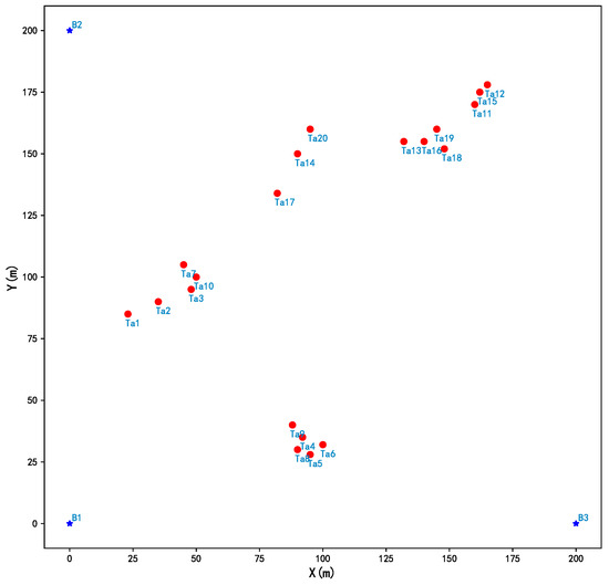
Figure 2. Initial bases and targets state.

Table 2. Information of three types of UAVs.

UAV	Base	${\mathbf{U}}_{\mathbf{resource}}$ (Units)		${\mathit{p}}_{\mathit{k}}$	${\mathit{p}}_{\mathit{s}}$
		a	b
Type A	B1	1	2	0.9	0.7
Type B	B2	2	2	0.8	0.8
Type C	B3	3	3	0.7	0.9

Table 3. Information of 20 targets.

Target	Position	${\mathbf{T}}_{\mathbf{resource}}$			y	s
		${\mathit{K}}_{\mathbf{1}}$ ([a,b])	${\mathit{K}}_{\mathbf{2}}$ ([a,b])	${\mathit{K}}_{\mathbf{3}}$ ([a,b])
Target 1	(23,85)	[2,3]	[2,3]	[2,3]	30	2
Target 2	(35,90)	[3,3]	[3,3]	[3,3]	70	6
Target 3	(48,95)	[2,3]	[2,3]	[2,3]	50	4
Target 4	(92,35)	[3,2]	[3,2]	[3,2]	100	10
Target 5	(95,28)	[2,2]	[2,2]	[2,2]	120	8
Target 6	(100,32)	[3,2]	[3,2]	[3,2]	40	5
Target 7	(45,105)	[3,3]	[3,3]	[3,3]	65	3
Target 8	(90,30)	[2,2]	[2,2]	[2,2]	78	7
Target 9	(88,40)	[2,2]	[2,2]	[2,2]	35	9
Target 10	(50,100)	[3,2]	[3,2]	[3,2]	63	5
Target 11	(160,170)	[2,3]	[5,3]	[4,3]	30	2
Target 12	(165,178)	[3,3]	[5,3]	[5,3]	70	6
Target 13	(132,155)	[3,3]	[5,3]	[6,3]	50	4
Target 14	(90,150)	[3,3]	[3,5]	[4,4]	100	10
Target 15	(162,175)	[2,2]	[4,5]	[4,4]	120	8
Target 16	(140,155)	[2,3]	[6,3]	[5,3]	40	5
Target 17	(82,134)	[3,3]	[4,3]	[4,3]	65	3
Target 18	(148,152)	[2,3]	[4,2]	[5,2]	78	7
Target 19	(145,160)	[3,2]	[3,4]	[4,3]	35	9
Target 20	(95,160)	[2,2]	[3,4]	[4,4]	63	5

Referring to Theorem 1, we note that when z exceeds 3, these simulations are complicated. Thus, z is set to be 3, i.e., no more than 3 UAVs are needed to accomplish three tasks of targets in a specific order, and then the total number of each type of UAV is unrestricted. Then, each target in the following cases has 19 possible schemes, i.e., A, B, C, $AA$, $AB$, $AC$, $BB$, $BC$, $CC$, $AAA$, $AAB$, $AAC$, $ABB$, $ACC$, $BBB$, $BBC$, $BCC$, $CCC$, and $ABC$, respectively, and these schemes correspond to numbers from 1 to 19. After that, we can use a matching approach to quickly find the feasible schemes. The resources needed to accomplish three tasks of targets are randomly generated and satisfy the maximum cooperative number of UAVs.

In the following simulations, the notations used in the tables and the figures are displayed as

• ${\mathrm{U}}_{\mathrm{resource}}$ represents the initial resources consumed by three types of UAVs;
• ${\mathrm{T}}_{\mathrm{resource}}$ represents the resources consumed by three tasks; and
• Time is CPU time in seconds for each case, and the time of each case is the average consumption time of running 100 times of each algorithm.

The parameters of the CE method, MIAFACE algorithm, MCAFACE algorithm, PSO algorithm, ACO algorithm, and GA algorithm are assumed to be set in Table 4, where the settings of the speed and maximum flying distance of the UAV are referred to [35] and they have no effect on the simulation results. For more detailed theory and parameter settings of CE, PSO, ACO, and GA (see [8,9,10,30,35,41]). For the targets in Table 3, there are two scenarios in the multi-UAV cooperative task assignment problem.

Table 4. Simulation parameter settings.

Parameter	Value
The target identification	$P_{\mathrm{c}}=1$
Weight coefficients	$w_1=0.8$, $w_2=0.18$, $w_3=0.02$
The UAV’s speed	$V=40$ m/s
The maximum flying distance	$D_{\max }=1000$ m
Time window of task $K_1$ (s)	$[{\mathrm{e}}_1,{\mathrm{s}}_1]=[3,10]$
Time window of task $K_2$ (s)	$[{\mathrm{e}}_2,{\mathrm{s}}_2]=[8,20]$
Time window of task $K_3$ (s)	$[{\mathrm{e}}_3,{\mathrm{s}}_3]=[18,26]$
Consumption time of task $K_1$	$T_1=5$ s
Consumption time of task $K_2$	$T_2=10$ s
Consumption time of task $K_3$	$T_3=5$ s
The number of targets	$N_{\mathrm{t}}\in [5,20]$
The fixed random samples	$N=1000$
The quantile in CE	$\theta =0.1$
Inertial weight in PSO	$w=0.75$
Learning factors in PSO	${\eta }_1={\eta }_2=0.5$
The number of ants in ACO	$N_{\mathrm{a}}=200$
Pheromone evaporation coefficient in ACO	$\epsilon =0.9$
Transfer probability in ACO	$P_{\mathrm{a}}=0.2$
Mating probability in GA	$P_1=0.8$
Mutation probability in GA	$P_2=0.01$

(1)

In scenario 1, we consider the first 10 targets or more similar targets. When performing the three tasks of each target, we obtain the identical optimal scheme vector of each task. Therefore, the situation in which each target has different tasks but each task has the same optimal scheme is called the problem with continuous and independent tasks.

(2)

In scenario 2, the last 10 targets or more similar targets are considered. When performing the three tasks of each target, we obtain the different optimal scheme vector of each task. Thus, the situation in which each target has different tasks and each task does not have the same optimal scheme is called the problem with continuous and correlative tasks.

5.1. Scenario 1

In case 1, we used the first 10 targets in Table 3 to perform continuous and independent tasks of problem $\mathcal{P}1$, and the results are shown in Table 5.

Table 5. Iterative results of three algorithms in case 1.

Algorithm	CE	MIAFACE	MCAFACE
Task	$K_1$	$K_1$	$K_1$
	$K_2$	$K_2$	$K_2$
	$K_3$	$K_3$	$K_3$
Iterations	4	3	3
			2
			1
Optimal scheme vector	[3,3,3,2,2,2,3,2,2,3]	[3,3,3,2,2,2,3,2,2,3]	[3,3,3,2,2,2,3,2,2,3]
			[9,9,9,7,7,7,9,7,7,9]
			[18,18,18,15,15,15,18,15,15,18]
Result of each task	−79.50	−79.50	−79.50
	274.90	274.90	179.0
	−79.50	−79.50	−82.14
Sum of each task’s result	115.9	115.9	17.36
Total time(s)	3.36	3.29	2.17

According to Table 5, we note that the optimal scheme vector and the total result of CE and MIAFACE are identical, while that of MCAFACE is suboptimal to the other two algorithms. Moreover, we can obtain some observations. (i) For CE, the number of iterations and the optimal scheme vector are both 4 and [3,3,3,2,2,2,3,2,2,3], respectively, and the results of each task are −79.50, 274.90, and −79.50, and the sum of the results of each task is 115.9. The situations of MIAFACE are similar to CE, except that the number of iterations is 3. (ii) For MCAFACE, the numbers of iterations and the optimal scheme vectors are 3, 2, 1 and [3,3,3,2,2,2,3,2,2,3], [9,9,9,7,7,7,9,7,7,9], [18,18,18,15,15,15,18,15,15,18], respectively, and the results of each task are −79.50, 179.0, and −82.14, and the sum of the results of each task is 17.36. (iii) The total times of using CE, MIAFACE and MCAFACE are 3.36, 3.29, and 2.17, respectively.

In case 2, we tested the MIAFACE algorithm and MCAFACE algorithm under h and ${\mathit{c}}_1$, and their times change with $N_{\mathrm{t}}$ in Figure 3a–c and Figure 4a–c, respectively.

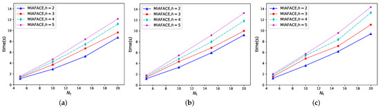
Figure 3. Time changing with $N_{\mathrm{t}}$ under MIAFACE algorithm in scenario 1. (a) ${\mathit{c}}_1$ = [0.01,0.02,0.03]. (b) ${\mathit{c}}_1$ = [0.02,0.03,0.04]. (c) ${\mathit{c}}_1$ = [0.03,0.04,0.05].

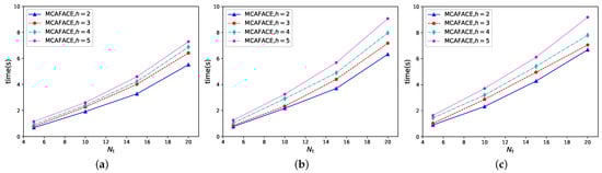
Figure 4. Time changing with $N_{\mathrm{t}}$ under MCAFACE algorithm in scenario 1. (a) ${\mathit{c}}_1$ = [0.01,0.02,0.03]. (b) ${\mathit{c}}_1$ = [0.02,0.03,0.04]. (c) ${\mathit{c}}_1$ = [0.03,0.04,0.05].

From Figure 3 and Figure 4, the curves of MIAFACE and MCAFACE both show an increasing trend as $N_{\mathrm{t}}$ grows, and their times increase with the increment of ${\mathit{c}}_1$ and h. Meanwhile, the time differences between the curves gradually increase with the growth of $N_{\mathrm{t}}$ in each figure. In Figure 3a, the curve with $h=2$ is at the lowest of the four curves, while the curve with $h=5$ is at the highest of the four curves. The remaining two curves are in the middle, and the curve with $h=4$ is at the top and the other one is at the bottom. Moreover, the time ranges of the four curves are both approximately in [1,12]. In Figure 3b,c, their situations are described similarly to Figure 3a, and their time ranges are in [1,14] and [1,15], respectively. From Figure 4a, the order of the four curves is similar to Figure 3a. Moreover, their time ranges are both roughly in [0.3,10]. In Figure 4b,c, their situations are analogous to Figure 4a, and their time ranges are in [0.3,10] and [0.3,12], respectively.

In case 3, the CE method, PSO algorithm, ACO algorithm, and GA algorithm are both used three times for three tasks continuously. We compared them with MIAFACE algorithm by obtaining the same optimal score under $h=2$ and ${\mathit{c}}_1$, and their times change with $N_{\mathrm{t}}$ in Figure 5a–c. Since MCAFACE algorithm obtains suboptimal results in scenario 1, it is not compared to other algorithms.

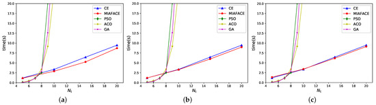
Figure 5. Time changing with $N_{\mathrm{t}}$ under $h=2$ and different algorithms in scenario 1. (a) ${\mathit{c}}_1$ = [0.01,0.02,0.03]. (b) ${\mathit{c}}_1$ = [0.02,0.03,0.04]. (c) ${\mathit{c}}_1$ = [0.03,0.04,0.05].

From Figure 5, we note that the curves of CE and MIAFACE grow linearly, while the curves of PSO, ACO, and GA increase exponentially. In addition, their times increase gradually with the increment of ${\mathit{c}}_1$ and $N_{\mathrm{t}}$. In Figure 5a, when $N_{\mathrm{t}}$ is in [5,20], the time of MIAFACE is less than that of CE, and the time difference between the two algorithms grows as $N_{\mathrm{t}}$ increases. Meanwhile, when $N_{\mathrm{t}}$ is below 8, the times of PSO, ACO, and GA are lower than that of CE and MIAFACE, but when $N_{\mathrm{t}}$ is more than 8, the situation is reversed. In addition, the time ranges of CE and MIAFACE are both approximately in [1,10], while the times of other algorithms are over 20 when $N_{\mathrm{t}}$ is larger than 10. From Figure 5b,c, their situations are similar to Figure 5a, except that the time difference between CE and MIAFACE in Figure 5b is lower than that in Figure 5a, and the time difference in Figure 5c first decreases gradually to intersect at a point where $N_{\mathrm{t}}$ is 10, then increases slowly with the increment of $N_{\mathrm{t}}$.

5.2. Scenario 2

In case 4, we utilized the last 10 targets in Table 3 to perform continuous and correlative tasks of problem $\mathcal{P}2$, and the results are shown in Table 6.

Table 6. Iterative results of three algorithms in case 4.

Algorithm	CE	MIAFACE	MCAFACE
Task	$K_1$	$K_1$	$K_1$
	$K_2$	$K_2$	$K_2$
	$K_3$	$K_3$	$K_3$
Iterations	5	4	4
			4
			3
Optimal scheme vector	[3,3,3,2,2,2,3,2,2,3]	[3,3,3,2,2,2,3,2,2,3]	[3,3,3,2,2,2,3,2,2,3]
	[9,9,9,7,7,7,9,7,7,9]	[9,9,9,7,7,7,9,7,7,9]	[9,9,9,7,7,7,9,7,7,9]
	[18,18,18,15,15,15,18,15,15,18]	[18,18,18,15,15,15,18,15,15,18]	[18,18,18,15,15,15,18,15,15,18]
Result of each task	−298.65	−298.65	−298.65
	819.85	819.85	819.85
	−302.48	−302.48	−302.48
Sum of each task’s result	218.72	218.72	218.72
Total time(s)	7.33	7.11	6.9

According to Table 6, we note that the optimal scheme vectors and the total results of CE, MIAFACE, and MCAFACE are the same. The reason for this phenomenon is that for three tasks of the same 10 targets, the optimal scheme vectors are eventually obtained and identical by using the three algorithms, which leads to the same score of the total objective function; however, the consumption time by the different algorithms varies. Moreover, some observations are available. First, for CE, the number of iterations and the sum of each task’s result are 5 and 218.72, and the optimal solution vectors are [3,3,3,3,3,3,3,3,3,3], [9,9,9,7,7,7,9,7,7,9], [18,18,18,15,15,15,18,15,15,18], and the results of each task are −298.65, 819.85, and −302.48, respectively. Secondly, the situations using MIAFACE and MCAFACE are similar to that of CE, apart from the fact that the number of iterations in MIAFACE is 4 and the numbers of iterations in MCAFACE are 4, 4, and 3. Finally, the total times using CE, MIAFACE, and MCAFACE are 7.33, 7.11, and 6.9, respectively.

In case 5, we tested the MIAFACE algorithm and MCAFACE algorithm under h and ${\mathit{c}}_2$, and their times change with $N_{\mathrm{t}}$ in Figure 6a–c and Figure 7a–c, respectively.

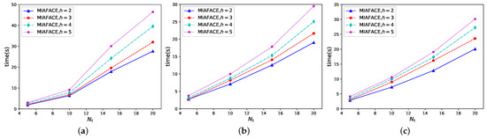
Figure 6. Time changing with $N_{\mathrm{t}}$ under MIAFACE algorithm in scenario 2. (a) ${\mathit{c}}_2$ = [0.01,0.02,0.03]. (b) ${\mathit{c}}_2$ = [0.02,0.03,0.04]. (c) ${\mathit{c}}_2$ = [0.03,0.04,0.05].

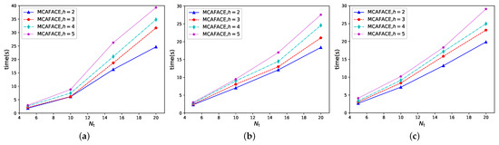
Figure 7. Time changing with $N_{\mathrm{t}}$ under MCAFACE algorithm in scenario 2. (a) ${\mathit{c}}_2$ = [0.01,0.02,0.03]. (b) ${\mathit{c}}_2$ = [0.02,0.03,0.04]. (c) ${\mathit{c}}_2$ = [0.03,0.04,0.05].

From Figure 6 and Figure 7, the variations of the curves, the times and the time differences are both similar to Figure 3 and Figure 4, while in Figure 6a and Figure 7a, the time grows rapidly when $N_{\mathrm{t}}$ is over 10. The reason is that the results of these two figures are suboptimal to others. In Figure 6a, the order of the curves is the same as that of each figure in Figure 3 and Figure 4. In addition, the time ranges of these four curves are both approximately in [1,50]. From Figure 6b,c, the situations are described similarly to that of Figure 6a and their time ranges are in [2,30] and [2,32], except that their results are the optimal results. In Figure 7, the situation of each figure is roughly similar to that of the corresponding figure in Figure 6, apart from the fact that the time range is lower than that in Figure 6.

In case 6, we compared the CE method, MIAFACE algorithm, MCAFACE algorithm, PSO algorithm, ACO algorithm, and GA algorithm by obtaining the same optimal score under $h=2$ and ${\mathit{c}}_2$, and their times change with $N_{\mathrm{t}}$ in Figure 8a–c. The CE method, PSO algorithm, ACO algorithm, and GA algorithm are also used three times for three tasks continuously.

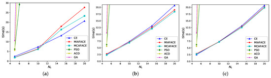
Figure 8. Time changing with $N_{\mathrm{t}}$ under $h=2$ and different algorithms in scenario 2. (a) ${\mathit{c}}_2$ = [0.01,0.02,0.03]. (b) ${\mathit{c}}_2$ = [0.02,0.03,0.04]. (c) ${\mathit{c}}_2$ = [0.03,0.04,0.05].

From Figure 8, we note that for CE, MIAFACE, MCAFACE, PSO, ACO, and GA, the variations of the curves and the times are similar to the case in Figure 5. In Figure 8a, when $N_{\mathrm{t}}$ is below 11, the times of MIAFACE and MCAFACE are relatively close and less than that of CE; however, when $N_{\mathrm{t}}$ is over 11, the times of MIAFACE and MCAFACE grow quickly and more than that of CE due to obtaining the suboptimal results. Moreover, the time ranges of CE, MIAFACE, and MCAFACE are both approximately in [1,30]. Meanwhile, the times of PSO, ACO, and GA are much higher than that of CE, MIAFACE, and MCAFACE, and their time ranges are over 30 when $N_{\mathrm{t}}$ is more than 6. From Figure 8b,c, the situations of PSO, ACO, and GA are similar to Figure 8a. In Figure 8b, the time differences between CE, MIAFACE, and MCAFACE grow as $N_{\mathrm{t}}$ increases. In addition, the time of MCAFACE is lower than that of CE and MIAFACE, and the curves of CE and MIAFACE intersect at $N_{\mathrm{t}}=8$ and the time of CE is also lower than that of MIAFACE when $N_{\mathrm{t}}$ is below 8, then the situation is reversed after $N_{\mathrm{t}}$ exceeds 8. Moreover, the time ranges of CE, MIAFACE, and MCAFACE are both in [2,22]. In Figure 8c, the time differences between CE, MIAFACE, and MCAFACE decrease, and then increase as $N_{\mathrm{t}}$ grows. Furthermore, the curves of CE, MIAFACE, and MCAFACE intersect at $N_{\mathrm{t}}=9$ and the time of CE is lower than that of MIAFACE and MCAFACE when $N_{\mathrm{t}}$ is below 9, then the situation is reversed after $N_{\mathrm{t}}$ exceeds 9.

5.3. Analysis

Analysing the results of case 1 and case 4, we note that the optimal scheme vectors of using MIAFACE and MCAFACE algorithms in problems $\mathcal{P}1$ and $\mathcal{P}2$, respectively, are obtained by initializing and updating the probability matrices $\mathit{P}(m)$ and $\mathit{Q}(m)$, which conforms to Algorithms 3 and 4 described in Section 4.2. In addition, the result of MCAFACE in case 1 is suboptimal to that of other algorithms due to deleting the corresponding optimal solution after the end of each task.

Comprehensively considering the situations of case 2 and case 5, we note that the times of CE, MIAFACE, and MCAFACE increase with the increment of $N_{\mathrm{t}}$, h, as well as $\mathit{c}$ and the time complexity of MCAFACE is lower than that of MIAFACE, and these phenomena comply with the complexity analysis of MIAFACE and MCAFACE in Section 4.3. In addition, the time of case 5 is superior to that of case 2 because there are more available solutions for each target in case 5 than in case 2 after each iteration. Meanwhile, in case 5, using MIAFACE and MCAFACE for solving this problem is easy to fall into local optimum when $\mathit{c}$ is inferior to a certain vector, e.g., $\mathit{c}=[0.01,0.02,0.03]$. The reason behind this phenomenon is that when all elements in $\mathit{c}$ are small and more solutions exist after each iteration, the optimal scheme may not be selected during one of the iterations of MIAFACE and MCAFACE, leading to a suboptimal result.

Comparing the situations of case 3 and case 6, we note that the times of PSO, ACO, and GA are only related to the growth of $N_{\mathrm{t}}$. Meanwhile, CE, MIAFACE, and MCAFACE are superior to PSO, ACO, and GA for large-scale allocation problems, e.g., more than 8 targets of case 3 and 5 targets of case 6. Moreover, CE is inferior to MIAFACE in scenario 1, e.g., Figure 5, when $N_{\mathrm{t}}$ is over 10. Moreover, e.g., Figure 8c in scenario 2, MCAFACE is superior to MIAFACE and CE when $N_{\mathrm{t}}$ is over 9.

6. Conclusions

In this paper, the multi-UAV cooperative task assignment problem was described and formulated, and three types of UAVs were considered, cooperatively accomplishing the classification, attack, and verification tasks of targets under resource, precedence, and timing constraints. After that, considering complex coupling among these three tasks, we decomposed the considered problem into two subproblems. In order to solve them, we proposed an AFACE algorithm, a MIAFACE algorithm, and a MCAFACE algorithm. Finally, simulation results verified that both MIAFACE and MCAFACE consume less time than other intelligent algorithms for solving the corresponding problem.

Nevertheless, there still exist challenges when applying the MIAFACE algorithm and MCAFACE algorithm to processing optimization problems, e.g., appropriate parameter settings, falling into local optimum when using lower elements in $\mathit{c}$, etc. In future work, it will be meaningful to concentrate on promoting these two algorithms on problems where it is vulnerable to local optimum when the number of samples is limited and on task assignment problems in complex dynamic scenarios.

References

- Singh, H.; Sharma, M. Electronic Warfare System Using Anti-Radar UAV. In Proceedings of the 2021 8th International Conference on Signal Processing and Integrated Networks, Noida, India, 26–27 August 2021; pp. 102–107. [Google Scholar]
- Deng, Z.; Gao, Y.; Hu, A.; Zhang, Y. A Mobile Phone Uplink CPDP-DTDOA Positioning Method Using UAVs for Search and Rescue. IEEE Sens. J. 2022, 22, 18170–18179. [Google Scholar] [CrossRef]
- Fan, B.; Jiang, L.; Chen, Y.; Zhang, Y.; Wu, Y. UAV Assisted Traffic Offloading in Air Ground Integrated Networks With Mixed User Traffic. IEEE T. Intell. Transp. 2022, 23, 12601–12611. [Google Scholar] [CrossRef]
- D’Arcy, S.; Gonzalez, F. Design and Flight Testing of a Rocket-Launched Folding UAV for Earth and Planetary Exploration Applications. In Proceedings of the 2022 IEEE Aerospace Conference, Big Sky, MT, USA, 5–12 March 2022; pp. 1–15. [Google Scholar]
- Chen, X.; Liu, Y.; Yin, L.; Qi, Y. Cooperative Task Assignment and Track Planning For Multi-UAV Attack Mobile Targets. J. Intell. Robot. Syst. 2020, 100, 1383–1400. [Google Scholar]
- Sabo, C.; Kingston, D.; Cohen, K. A Formulation and Heuristic Approach to Task Allocation and Routing of UAVs under Limited Communication. Unmanned Syst. 2014, 2, 1–17. [Google Scholar] [CrossRef]
- Wang, J.; Zhang, Y.F.; Geng, L.; Fuh, J.Y.H.; Teo, S.H. A Heuristic Mission Planning Algorithm for Heterogeneous Tasks with Heterogeneous UAVs. Unmanned Syst. 2015, 3, 205–219. [Google Scholar] [CrossRef]
- Gou, Q.; Li, Q. Task assignment based on PSO algorithm based on Logistic function inertia weight adaptive adjustment. In Proceedings of the 2020 3rd International Conference on Unmanned Systems, Harbin, China, 1–4 September 2020; pp. 825–829. [Google Scholar]
- Li, Y.; Zhang, S.; Chen, J.; Jiang, T.; Ye, F. Multi-UAV Cooperative Mission Assignment Algorithm Based on ACO method. In Proceedings of the 2020 International Conference on Computing, Networking and Communications, Big Island, HI, USA, 17–20 February 2020; pp. 304–308. [Google Scholar]
- Ma, Y.; Zhang, H.; Zhang, Y.; Gao, R.; Xu, Z.; Yang, J. Coordinated Optimization Algorithm Combining GA with Cluster for Multi-UAVs to Multi-tasks Task Assignment and Path Planning. In Proceedings of the 2019 IEEE 15th International Conference on Control and Automation, Edinburgh, UK, 22–26 August 2019; pp. 1026–1031. [Google Scholar]
- Duan, X.; Liu, H.; Tang, H.; Cai, Q.; Zhang, F.; Han, X. A Novel Hybrid Auction Algorithm for Multi-UAVs Dynamic Task Assignment. IEEE Access 2020, 8, 86207–86222. [Google Scholar] [CrossRef]
- Chen, J.; Wu, Q.; Xu, Y.; Qi, N.; Guan, X.; Zhang, Y.; Xue, Z. Joint Task Assignment and Spectrum Allocation in Heterogeneous UAV Communication Networks: A Coalition Formation Game-Theoretic Approach. IEEE Trans. Wirel. Commun. 2021, 20, 440–452. [Google Scholar] [CrossRef]
- Qie, H.; Shi, D.; Shen, T.; Xu, X.; Li, Y.; Wang, L. Joint Optimization of Multi-UAV Target Assignment and Path Planning Based on Multi-Agent Reinforcement Learning. IEEE Access 2019, 7, 146264–146272. [Google Scholar] [CrossRef]
- Tang, J.; Chen, X.; Zhu, X.; Zhu, F. Dynamic Reallocation Model of Multiple Unmanned Aerial Vehicle Tasks in Emergent Adjustment Scenarios. IEEE Trans. Aerosp. Electron. Syst. 2022, 1–43. [Google Scholar] [CrossRef]
- Qie, H.; Shi, D.; Shen, T.; Xu, X.; Li, Y.; Wang, L. Distributed Cooperative Search Algorithm With Task Assignment and Receding Horizon Predictive Control for Multiple Unmanned Aerial Vehicles. IEEE Access 2021, 9, 6122–6136. [Google Scholar]
- Fu, X.; Feng, P.; Gao, X. Swarm UAVs Task and Resource Dynamic Assignment Algorithm Based on Task Sequence Mechanism. IEEE Access 2019, 7, 41090–41100. [Google Scholar] [CrossRef]
- Chen, Y.; Yang, D.; Yu, J. Multi-UAV Task Assignment With Parameter and Time-Sensitive Uncertainties Using Modified Two-Part Wolf Pack Search Algorithm. IEEE Trans. Aerosp. Electron. Syst. 2018, 54, 2853–2872. [Google Scholar] [CrossRef]
- Zhu, F.; Wu, F.; Chen, C.F.; Li, D.; Guo, Y.; Zhang, J.G.; Zhao, X. A coordinated assignment method for multi-UAV area search tasks. In Proceedings of the CSAA/IET International Conference on Aircraft Utility Systems, Nanchang, China, 17–20 August 2022; pp. 751–756. [Google Scholar]
- Chen, Y.; Chen, J.; Du, C. Allocation of Multi-UAVs Timing-dependent Tasks based on Completion Time. In Proceedings of the 2022 WRC Symposium on Advanced Robotics and Automation, Beijing, China, 20 August 2022; pp. 71–76. [Google Scholar]
- Yan, S.; Xu, J.; Song, L.; Pan, F. Heterogeneous UAV collaborative task assignment based on extended CBBA algorithm. In Proceedings of the 2022 7th International Conference on Computer and Communication Systems, Wuhan, China, 22–25 April 2022; pp. 825–829. [Google Scholar]
- Yan, S.; Pan, F.; Zhang, D.; Xu, J. Research on Task Reassignment Method of Heterogeneous UAV in Dynamic Environment. In Proceedings of the 2022 6th International Conference on Robotics and Automation Sciences, Wuhan, China, 9–11 June 2022; pp. 57–61. [Google Scholar]
- Liu, C.; Guo, Y.; Li, N.; Song, X. AoI-Minimal Task Assignment and Trajectory Optimization in Multi-UAV-Assisted IoT Networks. IEEE Internet Things J. 2022, 9, 21777–21791. [Google Scholar] [CrossRef]
- Zhu, C.; Zhang, G.; Yang, K. Fairness-Aware Task Loss Rate Minimization for Multi-UAV Enabled Mobile Edge Computing. IEEE Wirel. Commun. Lett. 2023, 12, 94–98. [Google Scholar] [CrossRef]
- Seid, A.M.; Lu, J.; Abishu, H.N.; Ayall, T.A. Blockchain-Enabled Task Offloading with Energy Harvesting in Multi-UAV-assisted IoT Networks: A Multi-agent DRL Approach. IEEE J. Sel. Areas Commun. 2022, 40, 3517–3532. [Google Scholar] [CrossRef]
- Hu, N.; Qin, X.; Ma, N.; Liu, Y.; Yao, Y.; Zhang, P. Energy-efficient Caching and Task offloading for Timely Status Updates in UAV-assisted VANETs. In Proceedings of the 2022 IEEE/CIC International Conference on Communications in China, Sanshui, Foshan, China, 11–13 August 2022; pp. 1032–1037. [Google Scholar]
- Gao, H.; Feng, J.; Xiao, Y.; Zhang, B.; Wang, W. A UAV-assisted Multi-task Allocation Method for Mobile Crowd Sensing. IEEE Trans. Mob. Comput. 2022. [Google Scholar] [CrossRef]
- Rubinstein, R.Y. Optimization of computer simulation models with rare events. Eur. J. Oper. Res. 1997, 99, 89–112. [Google Scholar] [CrossRef]
- Rubinstein, R.Y. The cross-entropy method for combinatorial and continuous optimization. Methodol. Comput. Appl. Probab. 1999, 1, 127–190. [Google Scholar] [CrossRef]
- Rubinstein, R.Y. Combinatorial optimization, cross-entropy, ants and rare events. In Stochastic Optimization: Algorithms and Applications; Springer: Boston, MA, USA, 2001; pp. 303–363. [Google Scholar]
- De Boer, P.-T.; Kroese, D.P.; Mannor, S.; Rubinstein, R.Y. A tutorial on the cross-entropy method. Ann. Oper. Res. 2005, 134, 19–67. [Google Scholar] [CrossRef]
- Chepuri, K.; Homem-de-Mello, T. Solving the vehicle routing problem with stochastic demands using the cross-entropy method. Ann. Oper. Res. 2005, 134, 153–181. [Google Scholar] [CrossRef]
- Rubinstein, R.Y.; Kroses, D.P. The cross-entropy method: A unified approach to combinatorial optimization Monte-Carlo simulation and machine learning. Technometrics 2006, 48, 147–148. [Google Scholar]
- Undurti, A.; How, J. A Cross-Entropy Based Approach for UAV Task Allocation with Nonlinear Reward. In Proceedings of the AIAA Guidance, Navigation, and Control Conference, Toronto, ON, Canada, 2–5 August 2010; pp. 1–16. [Google Scholar]
- Le Thi, H.A.; Nguyen, D.M.; Dinh, T.P. Globally solving a nonlinear UAV task assignment problem by stochastic and deterministic optimization approaches. Optim. Lett. 2012, 6, 315–329. [Google Scholar] [CrossRef]
- Huang, L.; Qu, H.; Zuo, L. Multi-Type UAVs Cooperative Task Allocation Under Resource Constraints. IEEE Access 2018, 6, 17841–17850. [Google Scholar] [CrossRef]
- Cofta, P.; Ledziński, D.; Śmigiel, S.; Gackowska, M. Cross-Entropy as a Metric for the Robustness of Drone Swarms. Entropy 2020, 22, 597. [Google Scholar] [CrossRef] [PubMed]
- Zhang, X.; Wang, K.; Dai, W. Multi-UAVs Task Assignment Based on Fully Adaptive Cross-Entropy Algorithm. In Proceedings of the 2021 11th International Conference on Information Science and Technology, Chengdu, China, 7–10 May 2021; pp. 286–291. [Google Scholar]
- Wei, Y.; Wang, B.; Liu, W.; Zhang, L. Hierarchical Task Assignment of Multiple UAVs with Improved Firefly Algorithm Based on Simulated Annealing Mechanism. In Proceedings of the 2021 40th Chinese Control Conference, Shanghai, China, 26–28 July 2021; pp. 1943–1948. [Google Scholar]
- Wang, Q.; Liu, L.; Tian, W. Cooperative Task Assignment of Multi-UAV in Road-network Reconnaissance Using Customized Genetic Algorithm. In Proceedings of the 2021 IEEE 4th Advanced Information Management, Communicates, Electronic and Automation Control Conference, Chongqing, China, 18–20 June 2021; pp. 803–809. [Google Scholar]
- Costa, A.; Jones, O.D.; Kroese, D. Convergence properties of the cross-entropy method for discrete optimization. Oper. Res. Lett. 2007, 35, 573–580. [Google Scholar] [CrossRef]
- Kennedy, J.; Eberhart, R. Particle swarm optimization. In Proceedings of the ICNN’95—International Conference on Neural Networks, Perth, WA, Australia, 27 November–1 December 1995; pp. 1942–1948. [Google Scholar]
- Luo, Z.-Q.; Yu, W. An introduction to convex optimization for communications and signal processing. IEEE J. Sel. Areas Commun. 2006, 24, 1426–1438. [Google Scholar]
Disclaimer/Publisher’s Note: The statements, opinions and data contained in all publications are solely those of the individual author(s) and contributor(s) and not of MDPI and/or the editor(s). MDPI and/or the editor(s) disclaim responsibility for any injury to people or property resulting from any ideas, methods, instructions or products referred to in the content. |
© 2023 by the authors. Licensee MDPI, Basel, Switzerland. This article is an open access article distributed under the terms and conditions of the Creative Commons Attribution (CC BY) license (https://creativecommons.org/licenses/by/4.0/).