Abstract
Grassland biomass yield reflects a complex interaction of management intensity and environmental factors, yet quantifying the relative role of practices such as mowing and fertilization remains challenging. In this study, we introduce a multi-class machine learning framework to predict above-ground biomass on 150 permanent grassland plots across eight years (2009–2016) in Germany’s Biodiversity Exploratories and to evaluate the influence of key management variables. Following rigorous data cleaning, imputation of missing nitrogen values, feature standardization, and encoding of categorical practices, we trained CatBoost classifiers optimized via Bayesian hyperparameter search and mitigated class imbalance with ADASYN oversampling. We assessed model performance under binary, three-class, four-class, and five-class quantile-based categorizations, achieving test accuracies of 0.76, 0.57, 0.42, and 0.38, respectively. Across all schemes, mowing frequency and mineral nitrogen input emerged as the dominant predictors, while secondary variables such as drainage and conditioner use contributed as well. These results demonstrate that broad biomass categories can be forecast reliably from standardized management records, whereas finer distinctions necessitate additional environmental information or automated sensing to capture nonlinear effects and reduce reporting bias. This work shows both the potential and the limits of machine learning for informing sustainable grassland management and explainability thereof. Frequent mowing and higher mineral nitrogen inputs explained most of the predictable variation, enabling a 76% accurate separation of low and high biomass categories. Predictive accuracy fell below 60% for finer class resolutions, indicating that management records alone are insufficient for detailed yield forecasts without complementary environmental data.
1. Introduction
Grasslands play a crucial role in global ecosystems, serving as a primary source of forage for livestock, supporting biodiversity, and contributing to carbon sequestration [1,2]. Understanding the factors that influence grassland productivity is essential for optimizing land management practices, ensuring sustainable agricultural yields, and minimizing environmental impacts [3]. Nitrogen input and mowing frequency are widely recognized as major drivers of grassland biomass production, influencing both productivity and species composition [4,5]. The global rise in fertilizer use is largely driven by the need to sustain healthy biomass under increased mowing frequency, with improved yields further amplified by advancements in machinery and more efficient fertilization practices [6]. Nitrogen availability is a key limiting factor for primary productivity, directly influencing vegetative growth rates and biomass accumulation, but can lead to shifts in plant community composition, often promoting fast-growing, competitive species [7]. Mowing regimes, in turn, regulate regrowth dynamics and total biomass yield by periodically resetting plant developmental stages, reducing vertical structural complexity within the sward, which is, however, dependent on the plant species [8].
Machine learning (ML) offers tools to model complex, nonlinear relationships in agricultural data. ML and deep learning methods have been applied to forecasts in a diverse range of applications, e.g., in population studies, seizure prediction, and financial markets [9]. Within agriculture, ML models estimate crop yields and infer soil nitrogen status from field measurements [10]. Other examples of AI applications in agriculture can be found for supervised machine learning techniques in [11], for reinforcement learning in [12], and for unsupervised machine learning in [13,14].
In this study, we implement a multi-class ML pipeline to predict grassland biomass and to quantify the relative importance of management practices. Biomass is first grouped into two, three, four, and five classes using quantile-based thresholds. For each granularity, we train a CatBoost classifier—tuned via Bayesian optimization—and apply ADASYN oversampling to address class imbalance. We then evaluate model performance (accuracy, precision, recall, F1-score) on test and training sets, and extract feature importance scores to rank the influence of mineral and organic nitrogen inputs, mowing frequency, and other land use variables. This framework allows us to assess how predictive power varies with classification detail and which practices most strongly drive biomass yield.
1.1. Research Gap
Despite extensive use of machine learning techniques for biomass prediction—ranging from random forests to deep neural networks trained on remote sensing data—no study has combined a multi-class classification framework with a detailed feature importance analysis of management practices, as discussed in detail in Section 2. Our approach fills this gap by applying CatBoost across two to five biomass categories and quantifying the relative influence of mowing, mineral and organic nitrogen inputs, and other agronomic variables. Moreover, by evaluating model performance as class granularity increases, we clarify the limits of predicting yield outcomes from management records alone and identify which combinations of practices most reliably distinguish low, medium, and high biomass regimes.
1.2. Research Questions
Building on this gap, we address three research questions:
- 1.
- How accurately can ML models predict distinct biomass regimes, and which factors most strongly drive these predictions?
- 2.
- What is the relative influence of organic and mineral nitrogen inputs on biomass outcomes?
- 3.
- How do nitrogen inputs compare with mowing frequency and other management practices in determining biomass yield?
The remainder of the paper is organized as follows. Section 2 reviews related work. Section 3 describes the data, preprocessing steps, and ML methods. Section 4 presents classification performance and feature importance results. Section 5 summarizes conclusions and outlines future research directions.
2. Related Work
In the following section, we discuss two aspects of our approach: machine learning methods in agriculture, particularly to predict grassland biomass, and relevant publications from the Biodiversity Exploratories, which serve as the primary data source for this study.
Machine learning methods have been extensively applied to estimate biomass in various ecosystems, including grasslands and forests. Xu et al. [15] investigated the estimation of aboveground biomass (AGB) in degraded grasslands using terrestrial laser scanning (TLS). They evaluated several regression models—simple regression (SR), stepwise multiple regression (SMR), random forest (RF), and artificial neural networks (ANNs)—and found that SMR achieved the highest prediction accuracy, significantly influenced by minimum grass height and canopy coverage. Similarly, Wang et al. [16] analyzed 11 years of AGB data from the Three-River Headwaters Region, demonstrating that machine learning, particularly RF optimized through stepwise regression, effectively predicted grassland biomass across temporal and spatial scales. Their study highlighted the importance of variable selection for improving model accuracy. Peng and Karimi Sadaghiani [17] further extended the application of machine learning to forest biomass, illustrating its potential to enhance both quality and quantity through predictive modeling and decision support tools for forestry management.
Hyperspectral and remote sensing methods have become an important component in biomass estimation, offering scalable and efficient solutions for ecological monitoring. Huang et al. [18] combined hyperspectral remote sensing with various machine learning techniques to estimate grassland AGB in alpine meadows, identifying Gaussian process regression as the most accurate predictive model. Their work emphasized the improved predictive power achieved by combining spectral characteristics with temporal growth data. Complementing this, Morais et al. [19] reviewed the use of machine learning in combination with remote and proximal sensing data for grassland biomass estimation. They observed that prediction accuracy generally increased with sensor proximity and the number of field samples, although no single machine learning algorithm consistently outperformed the others. Finally, Shafizadeh et al. [20] applied machine learning to optimize hydrothermal liquefaction processes for biomass conversion, showing that Gaussian process regression could accurately predict optimal processing conditions. This body of research demonstrates the versatility and efficacy of machine learning in ecological biomass monitoring and optimization.
The Biodiversity Exploratories project, established in 2006, provides a comprehensive research platform to study interactions between land use, biodiversity, and ecosystem processes in forests and grasslands across Germany. With standardized data collection covering vegetation, soil, climate, and biodiversity, a wide range of research topics is addressed. Biomass estimation has been a central focus. Muro et al. [21] applied deep neural networks and remote sensing data, including Sentinel-1 and Sentinel-2, to predict grassland biomass and species richness, achieving improved prediction performance and robustness compared to conventional RF models.
Beyond biomass estimation, the Biodiversity Exploratories address broader ecological processes influenced by land use intensity. Künast et al. [22] examined the effects of mowing on arthropod populations, finding that some taxa are negatively affected while others benefit. Hartlieb et al. [23] developed an index to quantify mowing intensity, providing a tool for evaluating the relationship between grassland management and biodiversity. This tool can be integrated into the Land-Use Intensity (LUI) index by Blüthgen et al. [24], which combines mowing, grazing, and fertilization intensities. The LUI has shown that intensified land use reduces species and functional diversity across trophic levels, leading to ecological homogenization [25]. Collectively, these works illustrate the broad research scope of the Biodiversity Exploratories, contributing to the understanding of land use impacts on biodiversity and ecosystem functionality.
Despite extensive use of machine learning for biomass prediction—ranging from random forests to deep neural networks trained on remote sensing data—no study has combined a multi-class classification framework with a detailed feature importance analysis of management practices. Our approach fills this gap by applying CatBoost across two to five biomass categories and quantifying the relative influence of mowing, mineral and organic nitrogen inputs, and other agronomic variables. Moreover, by evaluating model performance as class granularity increases, we clarify the limits of predicting yield outcomes from management records alone and identify which combinations of practices most reliably distinguish low, medium, and high biomass regimes.
3. Methodology
This section details the experimental framework and machine learning techniques used to predict grassland biomass yield from fertilizer and mowing practice data. The methodology is implemented in Python, to automate data preprocessing, categorization, model training, evaluation, and logging of outputs. The full code is available in a corresponding GitHub repository: https://github.com/Raubkatz/Nitrogen_Classification (accessed on 1 April 2025).
- The Biodiversity Exploratories
Our data is obtained from the Biodiversity Exploratories, which are a long-term research platform, established in 2006, designed to explore the relationship between land use, biodiversity, and ecosystem processes within forest and grassland ecosystems [26]. The project involves standardized data collection on 300 plots, recording vegetation, soil parameters, climatic conditions, and various fauna and microbial communities. The studies are conducted across three distinct regions of Germany: the Schwäbische Alb (located in Baden-Württemberg, southwest Germany), the Hainich (in central Thüringen), and the Schorfheide-Chorin (in Brandenburg, northeast Germany). Our research focused on the 150 grassland plots—50 in each region—each spanning 50 m by 50 m. These plots encompass a wide range of land use intensities, from intense to minimally managed areas, and are situated within larger management units where land use practices are consistent. Approximately 35% of the plots are meadows, 35% grazed pastures, 27% mown pastures (which experience both grazing and mowing within the same year), and 3% left fallow. Fertilization was applied to about two-thirds of the meadows and mown pastures, but only 15% of the grazed pastures received fertilization [27].
3.1. The Dataset
Our analysis draws on two openly available data sets. The first is the biomass series, which reports annual dry-matter yield for all 150 permanent grassland plots from 2009 onward [28]. The second is the grassland management file released with [27]; it lists mowing, grazing and fertilizer inputs for the same plots from 2006 to 2016. Because the management file ends in 2016 and biomass sampling starts in 2009, the merged working table is limited to 2009–2016. The reason to choose these particular files is that they are openly available and thus accessible to us and other researchers who want to expand or reproduce this study.
3.1.1. Biomass Sampling
Each spring, eight sub-plots per plot were clipped to a 4 cm stubble before any land management activity between mid-May and mid-June. The harvested material was oven-dried at for 48 h and weighed to 0.01 g accuracy. The response variable is the mean dry mass per square meter [28,29].
3.1.2. Management Variables
Annual questionnaires completed by farmers record the number and timing of cuts, grazing pressure, machine type, conditioner use, and separate mineral and organic fertilizer amounts. Dung from grazing livestock is excluded from fertilizer totals. Nitrogen figures come from producer certificates or standard conversion factors. Overall, 116 variables are available for every plot-year between 2006 and 2016, from which we use a subset, as detailed in Table 1.

Table 1.
Features used as model inputs after cleaning.
3.1.3. Data Preprocessing and Cleaning
Both datasets include a unique identifier for each plot and the corresponding survey year. Biomass measurements were matched with features describing mowing and other management practices, forming a dataset where biomass serves as the target variable. Table 1 provides an overview of these features and the target variable.
Raw data is imported from a merged biomass and management practices file. The processing begins by removing non-informative features and discarding rows with missing target values. The remaining features are divided into numeric and categorical groups. Numeric features are standardized using a StandardScaler, which subtracts the mean and scales the data to unit variance. Missing values are kept as missing values except for nitrogen, which is discussed below.
Furthermore, biomass values are segmented into discrete categories using quantile-based thresholds. The script supports various classification schemes:
- Binary Classification: The mean value is used to distinguish between “low” and “high” biomass.
- Three-Class Classification: The 33rd and 66th percentiles define thresholds for “low”, “medium”, and “high” biomass.
- Four-Class Classification: The 25th, 50th, and 75th percentiles are used to assign four classes, typically labeled as “low”, “medium-low”, “medium-high”, and “high” biomass.
- Five-Class Classification: Quintiles (20%, 40%, 60%, 80%) are computed to assign labels “very_low”, “low”, “medium”, “high”, and “very_high” biomass.
In Table 1 we give a listing and brief description of the used variables to predict biomass quantiles from. Note that “org” and “min” refer to fertilizers of organic or mineral origin, respectively. Further details can be found in [27].
3.1.4. Fertilization Preprocessing
Accurate quantification of fertilizer-derived nutrients is essential for assessing grassland fertility; however, direct measurements are often incomplete or confounded by placeholder zeros. To avoid bias, we applied a uniform preprocessing rule to every fertilizer-related variable in the dataset:
NbFertilization, Manure_tha, Slurry_m3ha, orgNitrogen_kgNha, minNitrogen_kgNha, totalNitrogen_kgNha, minPhosphorus_kgPha, minPotassium_kgKha, Sulphur_kgSha
- Step 1: Remove non-positive entries. For each variable, values (including special codes such as −1) were set to missing.
- Step 2: Distinguish fertilized from non-fertilized samples. If the categorical field Fertilization was “no,” every fertilizer variable for that sample was left as missing. This prevents artificial zeros from compressing distribution ranges.
By removing spurious zeros, it preserves the natural spread of the fertilizer distributions and prevents downward bias in subsequent analyses.
3.2. Machine Learning
In this work, we used CatBoost, a widely utilized boosting algorithm [30,31]. Decision trees, which underlie boosting methods, are non-parametric supervised learning models that can handle both classification and regression tasks [32].
Boosting classifiers build on the principle of iteratively training multiple weak learners, typically shallow decision trees, and combining their predictions to form a robust ensemble. In contrast to bagging techniques, which train models independently and in parallel, boosting methods focus on errors identified at each iteration. Notable boosting frameworks include Random Forest [33], XGBoost [34], and LightGBM [35].
CatBoost implements gradient boosting with a permutation-based approach to handle categorical variables, minimizing the need for data transformation. It often achieves reliable accuracy across diverse applications with only minor hyperparameter adjustments [36,37]. CatBoost has also shown consistent results when utilizing complexity metrics and engineered features in domains such as software testing and particularly agriculture [11,38]. Its built-in GPU support further helps manage large-scale datasets.
To fine-tune parameters such as learning rate, tree depth, and regularization terms, we employed Bayesian optimization [39], a model-based method that seeks high-performance configurations while balancing exploration and exploitation. We automated this procedure using the scikit-opt Python package [40].
- Feature Importance Analysis
We conducted a feature importance analysis to determine how each feature influenced model predictions. This was carried out using CatBoost’s built-in functionality, which evaluates a feature’s impact on the model output [41].
Specifically, we applied the PredictionValuesChange method, which calculates the average variation in the predicted value when a particular feature is altered. This approach quantifies how the model’s output changes as feature values vary and is the default setting for non-ranking metrics. It helped us pinpoint the most significant features and offered insights into the relationships captured by the model.
- Train/Test Split and Scaling
The dataset is partitioned into training (90%) and validation (10%) sets using stratified sampling to maintain the class distribution. Numeric features in both sets are scaled with a StandardScaler fitted on the training data.
- Data Augmentation with ADASYN
To address class imbalance, the Adaptive Synthetic Sampling (ADASYN) algorithm is applied to the training set. The oversampling strategy is defined such that each class is upsampled to a target count determined by multiplying the majority class count by a specified OVERSAMPLE_FACTOR. ADASYN generates synthetic samples for classes based on the local feature space density, effectively balancing the dataset.
- Hyperparameter Tuning
A CatBoost classifier is utilized for all prediction tasks. To optimize its performance, Bayesian Optimization is performed using BayesSearchCV from the scikit-optimize library. The optimization is configured to run for 20 iterations with 3-fold cross-validation, targeting the maximization of accuracy. The best hyperparameter set identified during the search is then used to train the final model and tested against the out-of-the-box implementation of CatBoost. We do this because it is known that CatBoost’s out-of-the-box implementation already yields strong performances across various problems [37]. We then kept the optimized or out-of-the-box implementation based on their performance.
- Model Evaluation and Visualization
The best trained CatBoost model is evaluated on the validation set, the training set and the ADASYN-synthesized training set. Performance is quantified using accuracy metrics, a detailed classification report, and a confusion matrix. All feature importances are calculated from the CatBoost model and visualized as a bar plot, providing insights into the relative contributions of each feature to the biomass prediction.
- Overview Experimental Setup
The key points of our experimental design are depicted in Figure 1 and detailed in the following:
- 1.
- Data Loading and Cleaning: Load the raw dataset, remove irrelevant columns, and handle missing values.
- 2.
- Feature Engineering: Separate features into numeric and categorical sets, standardize numeric variables, and encode categorical variables.
- 3.
- Biomass Categorization: Compute quantile-based thresholds and assign biomass observations to binary, three, four, or five classes.
- 4.
- Data Splitting and Scaling: Split the data into training and validation sets; fit a StandardScaler on the training set and apply it to both sets.
- 5.
- Oversampling: Use ADASYN to generate synthetic samples for minority classes and balance the training set.
- 6.
- Hyperparameter Optimization and Training: Perform Bayesian Optimization with BayesSearchCV to tune CatBoost hyperparameters on the ADASYN training data, then train the final model.
- 7.
- Validation and Analysis: Evaluate each model’s accuracy and other metrics on the original training set, the ADASYN-augmented training set, and the validation set. Generate confusion matrices, classification reports, distribution plots for nitrogen-related features, and extract feature importance scores.

Figure 1.
Overview of the experimental pipeline. Starting from raw grassland management and biomass data, we perform cleaning and quantile-based categorization into two to five classes. The training set is then upsampled using ADASYN, and a CatBoost classifier is trained to predict biomass categories. Finally, we evaluate model performance on test, original, and augmented training sets using classification reports, confusion matrices, feature importance rankings, and distribution plots of key predictors.
4. Results and Discussion
This section presents the outcomes of our classification experiments, comparing performance across four quantile-based schemes (binary, three-class, four-class, and five-class). For each scheme, we report accuracy, precision, recall, and F1-scores on test, augmented, and original training sets. We then examine how predictive performance changes as class granularity increases, and identify the best-performing models under default and Bayesian-optimized hyperparameters.
Feature importance results are presented to highlight the relative influence of mowing frequency, mineral and organic nitrogen inputs, and other management variables. Finally, we interpret these findings in light of similar studies, discuss potential sources of bias—such as imputation effects—and outline limitations and directions for future improvement.
4.1. Preliminary Evaluation
To examine relationships between management practices and biomass yield, we perform an initial exploratory analysis using quantile-based class definitions. For each of the four classification schemes (binary, three-class, four-class, and five-class), biomass values were divided according to the relevant quantile thresholds. We generated boxplots of mowing frequency, mineral nitrogen input (minNitrogen_kgNha), total nitrogen input (totalNitrogen_kgNha), and organic nitrogen input (orgNitrogen_kgNha) for each biomass class (Figure 2, Figure 3, Figure 4 and Figure 5).
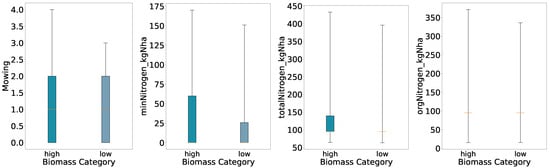
Figure 2.
Distributions of key features for predicted categories (two quantiles, full whisker range).
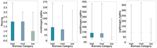
Figure 3.
Distributions of key features for predicted categories (three quantiles, full whisker range).
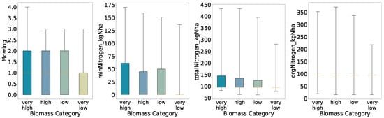
Figure 4.
Distributions of key features for predicted categories (four quantiles, full whisker range).
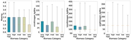
Figure 5.
Distributions of key features for predicted categories (five quantiles, full whisker range).
These visualizations facilitated a clear comparison of feature distributions across increasing biomass levels.
Overall, the preliminary analysis reveals that mowing frequency and nitrogen inputs generally increase with higher biomass classes under coarse segmentation (binary and three-class schemes). As class granularity increases, the spreads broaden almost monotonically up to four classes, indicating consistent positive relationships between inputs and yield. In the five-class scheme, however, the interquartile ranges for mineral and total nitrogen inputs in the High class narrow relative to the Medium class, suggesting that at finer resolution the relationship between nitrogen application and biomass yield becomes more complex and non-linear.
With a binary split the High class shows wider full ranges for all four variables than the Low class. The boxes for orgNitrogen_kgNha and the lower end of totalNitrogen_kgNha nearly collapse at the median, meaning that when organic nitrogen was applied as a fertilizer, farmers used mostly the same amount, with some rare events of drastically high amounts of fertilizer and many plots not applying any organic nitrogen (i.e., zero).
Using three quantiles, both High and Medium retain broader inter-quartile ranges for all variables, while the Low class remains compact for all features. Here we further see decreased ranges and interquartile ranges for low yields, supporting the previous findings for the binary biomass categories; increased amounts of mowing and nitrogen fertilization accompany increased biomass.
With four quantiles the spread increases almost monotonically from Very Low through Very High; only the Low group deviates slightly. Further, for mineral nitrogen we see a deviation in the interquartile ranges for the high biomass class, i.e., the high biomass class has a slightly lower interquartile range than the low biomass class.
At five quantiles the pattern becomes non-monotonic; for minNitrogen_kgNha and totalNitrogen_kgNha the inter-quartile range of the High class is narrower than that of the Medium class. This indicates a more complex, non-linear relationship in which additional nitrogen does not always lead to higher biomass once the classes are defined more finely.
4.2. Results of Binary Quantile Classification
Dividing biomass into Low and High classes at the median yields robust discrimination. On the test set (Table 2), overall accuracy reaches 0.7667. Precision for the High class is 0.72, with a recall of 0.69 (34 of 49 correctly identified), while the Low class attains precision 0.79 and recall 0.82 (58 of 71 correctly identified). The macro-averaged F1-score of 0.76 indicates balanced performance across classes. Confusion matrices (Figure 6) reveal that most errors consist of High samples misclassified as Low (15 of 49) rather than the reverse, a pattern consistent across original and ADASYN-augmented training sets, where accuracy remains near 0.76–0.77. This suggests the model is slightly conservative in assigning the High label but maintains overall stability after oversampling.
Table 2.
Binary quantile classification report.
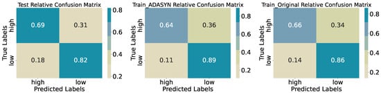
Figure 6.
Confusion matrices for training, synthetic training, and test sets (binary quantiles).
For the distribution of the predicted classes of mowing and nitrogen (Figure 7), we see similar behavior as for the initial evaluation, shown in Figure 2; however, for the predicted classes the differences in the distribution for Mowing and minNitrogen_kgNha are much more pronounced. This indicates that the behavior the model learned from the data is that increased mowing intensity and increased mineral nitrogen applied lead to increased yields. Both distributions for organic nitrogen and total nitrogen look very similar to the initial evaluation; however, particularly for total nitrogen we see an increased median in the boxplots of the distribution, which accords with the previous findings of a more pronounced increase in mineral nitrogen for the high-yield regime, as total nitrogen is just the sum of organic and mineral nitrogen.
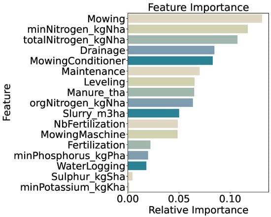
Figure 7.
Feature importance for binary quantile classification.
Feature importance analysis (Figure 8) highlights mowing frequency as the strongest predictor (13.1%), followed by mineral nitrogen input (minNitrogen_kgNha, 11.7%) and total nitrogen input (totalNitrogen_kgNha, 10.7%). Drainage application (8.5%) and the use of a mowing conditioner (8.3%) also contribute substantially. Lower importance scores for secondary variables—such as phosphorus input (2.0%) and a generic fertilization indicator (2.2%)—indicate that precise nitrogen measures and specific management practices drive model decisions. Overall, the prominence of mowing and nitrogen features confirms that both mechanical and nutrient inputs are key determinants of end-of-season biomass under a coarse, two-class framework.
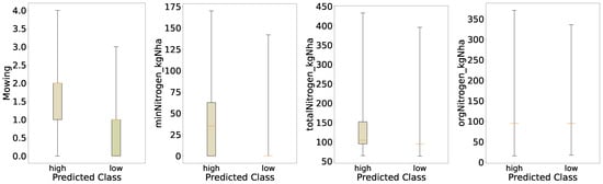
Figure 8.
Distributions of key features for predicted categories (binary quantiles).
4.3. Results of Three-Quantile Classification
The three-class model attains an accuracy of 0.5833 on the test set (Table 3). Precision and recall vary substantially across classes; the High class achieves 0.66 precision and 0.64 recall (25 of 39 correctly identified), the Low class reaches 0.55 precision and 0.88 recall (36 of 41), while the Medium class lags with 0.56 precision and 0.23 recall (9 of 40). The confusion matrix (Figure 9) shows that 22 of 40 true Medium samples are misclassified as Low, and 9 as High, indicating substantial overlap in feature distributions at intermediate biomass levels. On the original training data, accuracy is 0.6788 with medium recall 0.48, and ADASYN oversampling raises training accuracy to 0.7129 and medium recall to 0.53, though the medium class remains the most error-prone. This difference in training and testing accuracies and performance shows that the model is overfitted on the training data and the model does not generalize well for predicting three quantiles of biomass regimes.
Table 3.
Three-quantile classification report.
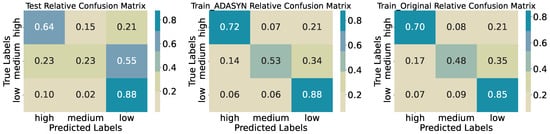
Figure 9.
Confusion matrices for training, synthetic training, and test sets (three quantiles).
For the distribution of the predicted classes of mowing and nitrogen (Figure 10), we see similar behavior to the initial evaluation, shown in Figure 3; however, for the predicted classes the differences in the distributions of Mowing and minNitrogen_kgNha are changed. First, the medians are shifted for the medium biomass class, i.e., we see increased medians for mowing, mineral, and organic nitrogen in the medium class. Further, the medium biomass class shows a decreased interquartile range for mowing, pointing toward reduced variation in biomass for regimes with, on average, more cuts per year. We see similar behavior for mineral nitrogen: an increased median for the medium class and an increased interquartile range, indicating that the highest biomass is not necessarily linked to the highest amount of mineral nitrogen applied to the fields.
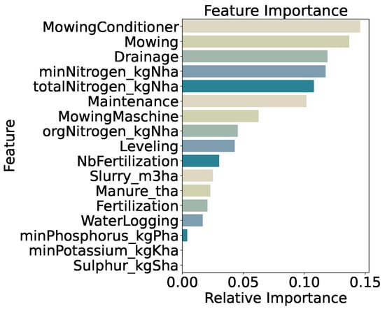
Figure 10.
Feature importance for three-quantile classification.
Feature importance for the three-class model (Figure 11) is led by use of a mowing conditioner (14.6%), mowing frequency (13.7%), and drainage application (11.9%). Mineral nitrogen input (minNitrogen_kgNha, 11.7%) and total nitrogen input (totalNitrogen_kgNha, 10.8%) are also highly ranked, with general maintenance practices (10.2%) following. The prominence of these management-related features confirms that mechanical disturbance and precise nutrient inputs drive differentiation among low, medium, and high biomass classes, while lower-ranked variables contribute marginally to model decisions.
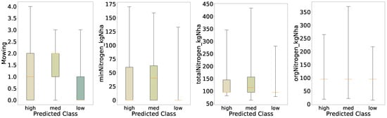
Figure 11.
Distributions of key features for predicted categories (three quantiles).
4.4. Results of Four-Quantile Classification
Dividing biomass into four classes (very_low, low, high, very_high) yields a test accuracy of 0.4250 (Table 4). Performance varies markedly by class; very_high achieves precision 0.57 and recall 0.47, while very_low reaches precision 0.45 and recall 0.59. The middle classes fare worse—high records precision 0.21 and recall 0.33; low has precision 0.42 and recall 0.28—resulting in a macro-averaged F1-score of 0.41.
Table 4.
Four-quantile classification report.
The confusion matrices (Figure 12) show frequent misclassification between adjacent classes. Only 33% of true high samples are correctly identified, with 27% mislabelled as very_high and 27% as very_low. Similarly, 44% of true low samples are predicted as very_low, indicating limited separation in the feature space at intermediate biomass levels. On the original training set, accuracy rises to 0.6153, with recall 0.70 for very_high and 0.78 for very_low. ADASYN oversampling further increases training accuracy to 0.6692 and recall across classes (very_high: 0.73; high: 0.54; low: 0.56; very_low: 0.84), though the high class remains challenging. Again, as for the three-quantile classification, this shows that the model does not generalize well, as the performance drops sharply for the test data set, meaning that the model overfits the training data.
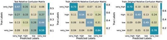
Figure 12.
Confusion matrices for training, synthetic training, and test sets (four quantiles).
Again, the distributions of the predicted four-class results (Figure 13) are similar to the initial distributions (Figure 4); however, we observe narrower interquartile ranges for the high and low classes in terms of mowing intensity per year, and an increased median—particularly for the high class—compared with the initial evaluation. A further difference is that the low-biomass class shows a very low median for mineral nitrogen input. Mineral nitrogen also lost feature importance relative to the binary classification, which means the class differences are less distinct for this variable within the model. We see slightly similar behavior for total nitrogen, as it is linked to mineral nitrogen, while organic nitrogen remains mostly unchanged. Moreover, the model does not generalize well and appears overfitted; we therefore conclude that these deviations for the non-extreme classes mark areas where the model fails to account for variation.
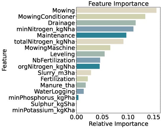
Figure 13.
Feature importance for four-quantile classification.
Feature importance (Figure 14) is led by mowing frequency (15.5%) and use of a mowing conditioner (13.4%), followed by drainage (11.5%), mineral nitrogen input (minNitrogen_kgNha, 11.1%), general maintenance practices (9.7%), and total nitrogen input (9.1%). Distributions of these features across classes (Figure 14) show generally increasing medians and interquartile ranges from very_low to very_high, confirming that both mechanical disturbance and nutrient inputs remain the primary drivers of biomass even under finer class segmentation.
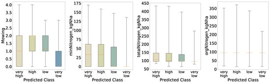
Figure 14.
Distributions of key features for predicted categories (four quantiles).
4.5. Results of Five-Quantile Classification
Splitting biomass into five quantile-based classes yields a test accuracy of 0.3250 (Table 5). Precision and recall vary substantially across classes; very_high achieves precision 0.59 and recall 0.36, while very_low attains precision 0.39 and recall 0.64. The intermediate classes perform poorly—high has precision 0.15, recall 0.18; medium and low register recalls of 0.21 and 0.19, respectively—resulting in a macro-averaged F1-score of 0.31. Confusion matrices (Figure 15) reveal that many true high and medium instances are misclassified into adjacent categories (e.g., 29% of high as medium, 24% as very_high; 33% of medium as very_low), indicating limited separability at finer granularity. Training accuracy improves to 0.5621 on the original data and to 0.6237 with ADASYN oversampling, yet misclassification patterns persist, particularly among the middle three classes.
Table 5.
Five-Quantile classification report.
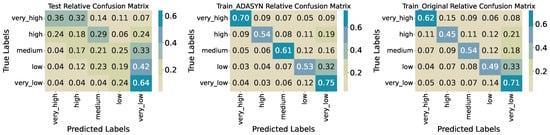
Figure 15.
Confusion matrices for training, synthetic training, and test sets (five quantiles).
Feature importance for the five-class model (Figure 16) remains dominated by management variables; mowing frequency (15.9%) and use of a mowing conditioner (13.8%) together account for nearly 30% of total importance. Drainage (12.4%) and mineral nitrogen input (minNitrogen_kgNha, 12.2%) follow, with general maintenance (9.4%) and total nitrogen input (totalNitrogen_kgNha, 8.8%) also contributing. The relative decline in importance of nitrogen features compared to the two- and three-class models suggests that at very fine biomass resolution, mechanical management practices drive most of the predictive signal. Distributions of these top features across quantile classes (Figure 17) show progressively increasing medians and interquartile ranges from very_low to very_high, confirming their central role even under challenging classification conditions.
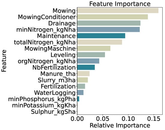
Figure 16.
Feature importance for five-quantile classification.
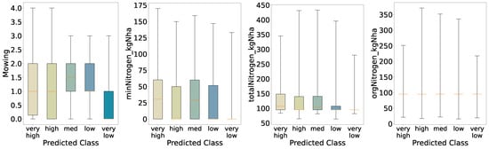
Figure 17.
Distributions of key features for predicted categories (five quantiles).
Once more, the distributions obtained from the five-class predictions (Figure 17) resemble those from the initial analysis (Figure 5) and the four-quantile scheme; nevertheless, the medium and low groups exhibit tighter interquartile ranges for annual mowing intensity and a higher median—most pronounced in the medium class—than in the initial evaluation. Another notable change is that the very high biomass class displays a low median for mineral nitrogen input. This suggests that the model inferred a link between reduced mineral nitrogen and increased biomass. Again, consistent with this, mineral nitrogen has lost feature importance relative to the binary classification, so class contrasts for this variable are less sharp. Total nitrogen follows a broadly similar pattern, as it depends on mineral nitrogen, whereas organic nitrogen remains largely unchanged. Finally, because the model does not generalize well and appears overfitted, we interpret these shifts in the non-extreme classes as signs of where the model fails to capture underlying variability.
4.6. Discussion
Our experiments demonstrate that machine learning can reliably distinguish broad biomass yield categories from standardized grassland management data, but that predictive power diminishes as class granularity increases. In the binary classification (Table 2), the CatBoost model achieved 77% accuracy on unseen data. Mowing frequency and mineral nitrogen input together accounted for just under 25% of feature importance (Figure 7), confirming that both mechanical disturbance and precise nutrient inputs are primary drivers of overall biomass. The high ranking of mowing conditioner and drainage variables further indicates that intensive management regimes—characterized by frequent cutting, use of conditioners, and effective water control—are strongly associated with higher yields.
When the task was extended to three classes, accuracy fell to 58% (Table 3). The confusion matrix (Figure 9) reveals that the Medium class overlaps substantially with both Low and High, resulting in only 23% recall for medium yields. This reflects the preliminary distribution analysis (Section 4.1), where interquartile ranges for key features in the medium class remained relatively broad and similar over all classes. Moving to four and five classes further reduced accuracy to 42% and 33%, respectively (Table 4 and Table 5). In these finer schemes, misclassifications occur predominantly between adjacent categories, e.g., true high yields labeled as very_high or low, indicating that small differences in management inputs do not translate into clear class separations.
It is noteworthy that, for all schemes beyond the binary classification, accuracy drops substantially from training to test data. This suggests overfitting to the training samples rather than capture of underlying relationships between management practices and biomass outcomes. Consequently, our binary classification results—and the associated feature importance rankings—are the most reliable. In that model, mowing frequency and mineral nitrogen input emerge as the dominant drivers of increased biomass. Total nitrogen (the sum of organic and mineral nitrogen) ranks third, but organic nitrogen alone never appears among the top five features, indicating that the mineral component drives its importance. Although existing studies highlight the role of soil/organic nitrogen in plant-based crop rotation planning and overall soil fertility (e.g., [12,42,43]), our findings cannot rule out its true influence; rather, they underscore the need for more complete data on organic nitrogen application.
Despite declining accuracy and generalizability, feature importance patterns remained stable across the three- to five-class schemes (Figure 10, Figure 11, Figure 12, Figure 13, Figure 14, Figure 15 and Figure 16). Mowing frequency and conditioner use consistently ranked highest, followed by drainage, mineral nitrogen input, and general maintenance. This suggests that, even when precise class assignments are unreliable, these core practices dominate the available information on biomass regimes. However, given the low accuracy and limited generalizability, these importance scores most likely reflect strong patterns in the training data rather than true causal effects.
Secondary features—such as phosphorus input and binary fertilization flags—contributed minimally across all schemes, implying that precise, quantitative measures of nitrogen and exact mowing records carry more predictive value than simple categorical indicators.
Compared to regression or correlation analyses, our multi-class classification approach offers two key advantages. First, it quantifies classification limits; the stepwise decline in test accuracy with increasing class number (77% → 58% → 42% → 33%) defines how much yield detail can be inferred from management logs. Second, it provides direct measures of model confidence for each class—valuable for advisory purposes where broad categories (e.g., “low” vs. “high” yield) can be forecast reliably, while finer distinctions are gradually more difficult.
Data quality and completeness remain major constraints. Monotonic values in fertilization measurements compress distribution ranges (Section 3.1.4) and may bias importance estimates, particularly for organic nitrogen. Agricultural data acquisition is resource-intensive and methods evolve rapidly, making long-term consistency challenging. Beyond farmer questionnaires, valuable data sources now include (i) satellite imagery such as Sentinel-2 and Landsat-9 for annual to decadal coverage, (ii) UAV multispectral or hyperspectral surveys that capture sub-plot nitrogen status and canopy traits, (iii) LiDAR for three-dimensional biomass and surface roughness, (iv) on-board yield monitors on harvesters, and (v) ground-based IoT probes that stream soil moisture, temperature, and mineral nitrogen in real time [44,45,46,47]. UAV-derived red-edge and chlorophyll indices have already estimated leaf nitrogen concentration with a root-mean-square error (RMSE) below 1.5 mg g−1 for winter wheat [48]. Integrating these sources with local weather stations, and potentially other data sources, will enlarge spatial and temporal coverage, reduce reliance on self-reported inputs, and support site-specific fertilizer decisions. Thus, future work should integrate automated sensing (e.g., drone-based hyperspectral imaging, in-field robotic probes) to obtain continuous, objective measurements of nutrient status and soil moisture, reduce reliance on farmer-reported entries, and improve spatial and temporal coverage.
5. Conclusions
This study applied a multi-class machine learning pipeline to predict grassland biomass yield from detailed management records collected by the Biodiversity Exploratories. Using CatBoost classifiers tuned via Bayesian optimization and balanced with ADASYN oversampling, we achieved robust separation of low versus high biomass (77 % accuracy) and progressively finer, though less reliable, classification into three (58 %), four (42 %), and five (33 %) quantile-based classes. Across all schemes, mowing frequency and precise nitrogen inputs—particularly mineral nitrogen and total nitrogen—emerged as the dominant drivers of biomass variability, together accounting for just under one quarter of the total feature importance in the binary model. Secondary management factors (e.g., conditioner use, drainage) contributed meaningfully, whereas broad nutrient indicators (e.g., binary fertilization flags, phosphorus input) offered limited additional predictive value.
Using the same pipeline, we again observed that, beyond the binary split, model accuracy dropped substantially from the training to the test set, indicating limited generalizability and a tendency to overfit the training data when class granularity increased. Across all schemes and particularly for the binary model, mowing frequency and nitrogen inputs—especially mineral nitrogen and total nitrogen—are dominant drivers of biomass variability, together accounting for nearly one quarter of the total feature importance. Secondary management factors (e.g., conditioner use, drainage) contributed meaningfully, whereas broad nutrient indicators (e.g., binary fertilization flags, phosphorus input) offered limited additional predictive value.
Our results quantify the practical limits of predicting fine-grain yield categories from farmer-reported management data alone. The decline in accuracy with increasing class number highlights nonlinear and threshold effects in the input–yield relationship, and indicates that subsampling errors and missing values introduce additional uncertainty at intermediate yield levels. To improve precision for three-class and finer schemes, future work should integrate complementary environmental covariates—such as soil moisture, weather data, or plant species composition—and employ automated sensing technologies (e.g., drone-mounted hyperspectral imagery, in-field soil probes) to capture key variables more objectively and at higher resolution.
These findings also have direct implications for grassland management. The clear dichotomy between high-intensity regimes (frequent mowing, high nitrogen input) and low-intensity regimes suggests distinct farmer strategies. Advisory services or incentive schemes could target mid-intensity practitioners to optimize yield without excessive inputs.
- Research Questions Answered
Based on our results, we address the three research questions as follows:
- 1.
- Prediction accuracy and key drivers: Machine learning models can predict broad biomass regimes (binary split) with good accuracy (77%) and clearly identify key drivers, but their reliability declines with finer class granularity.
- 2.
- Influence of nitrogen inputs: Mineral nitrogen input consistently ranks among the top predictors; while organic nitrogen’s role cannot be fully assessed due to data limitations, total nitrogen remains an important feature.
- 3.
- Comparison of management factors: Mowing frequency and mineral nitrogen inputs outweigh other management practices in determining biomass yield, with secondary factors (e.g., drainage, maintenance) providing additional, but smaller, predictive value.
To the best of our knowledge, this is the first study that (i) applies a multi-class CatBoost framework—tuned by Bayesian optimization and balanced with ADASYN—to grassland biomass prediction, (ii) couples those predictions with a systematic, model-intrinsic feature importance ranking of mowing and fertilizer variables, and (iii) quantifies how both accuracy and variable relevance decline step-wise as class granularity increases from two to five categories. By working only with farmer-reported management data and an eight-year, plot-level time series, we show the practical resolution limit of such records and provide a workflow that can be transferred to other long-term ecological datasets or extended with remote sensing covariates in future work.
Consequently, this study highlights the value of long-term, standardized datasets like the Biodiversity Exploratories, while underscoring the need for improved data protocols and novel sensing technologies to capture soil variables more completely. By combining robust field experiments with advanced machine learning and automated sensing, future research can develop more precise and sustainable grassland management strategies.
Author Contributions
Conceptualization, S.R., M.H. and K.M.; methodology, S.R.; software, S.R. and K.M.; validation, S.R., M.H., P.K. and K.M.; formal analysis, S.R.; investigation, S.R.; resources, M.H.; data curation, S.R. and J.H.; writing—original draft preparation, S.R., M.H., K.M. and P.K.; writing—review and editing, M.H., P.K. and K.M.; visualization, S.R.; supervision, M.H. and K.M.; project administration, K.M.; funding acquisition, K.M., S.R. and M.H. All authors have read and agreed to the published version of the manuscript.
Funding
The Biodiversity Exploratories (BE) are a research project funded by Deutsche Forschungsgemenischaft (DFG Priority Program 1374).
Institutional Review Board Statement
Not applicable.
Informed Consent Statement
Not applicable.
Data Availability Statement
All code used in this study is publicly available in the corresponding GitHub repository: https://github.com/Raubkatz/Nitrogen_Classification, accessed on 1 April 2025. Reproducibility is further ensured through the use of openly accessible datasets. Biomass data were sourced from [29] and can be downloaded via the BEXIS database at https://www.bexis.uni-jena.de/ddm/data/Showdata/31448, accessed on 1 April 2025. Grassland management data are from [27] and are available on the project’s data portal: https://bdj.pensoft.net/article/36387/element/4/5226558//, accessed on 1 April 2025. Together, these resources provide a fully transparent foundation for replicating and extending our findings.
Acknowledgments
SBA Research (SBA-K1 NGC) is a COMET Center within the COMET – Competence Centers for Excellent Technologies Programme and funded by BMIMI, BMWET, and the federal state of Vienna. The COMET Programme is managed by FFG. We would like to thank the Interviewers: Juliane Vogt, Anna Franke, Manfred Ayasse, Miriam Teuscher, Robert Künast, Ralf Lauterbach, Sonja Gockel, Claudia Seilwinder, Steffen Both, Niclas Otto, Christin Schreiber, Uta Schumacher, Stephan Getzin, as well as Metke Lilienthal, who also contributed in the development of the questionnaire for the information of the land use. We thank the staff of the three exploratories, the BE office and the BExIS team for their work in maintaining the plot and project infrastructure, and Markus Fischer, the late Elisabeth Kalko, Eduard Linsenmair, Dominik Hessenmöller, Jens Nieschulze, Daniel Prati, Ingo Schöning, François Buscot, Ernst-Detlef Schulze and Wolfgang W. Weisser for their role in setting up the Biodiversity Exploratories project. The financial support by the Austrian Federal Ministry of Labour and Economy, the National Foundation for Research, Technology and Development and the Christian Doppler Research Association is gratefully acknowledged.
Conflicts of Interest
The authors declare no conflicts of interest.
Correction Statement
This article has been republished with a minor correction to the reference 28. This change does not affect the scientific content of the article.
Abbreviations
The following abbreviations are used in this manuscript:
| ADASYN | Adaptive Synthetic Sampling Approach |
| CAT | CatBoost |
| BO | Bayesian Optimization |
| ML | Machine Learning |
References
- O’Mara, F.P. The role of grasslands in food security and climate change. Ann. Bot. 2012, 110, 1263–1270. [Google Scholar] [CrossRef] [PubMed]
- Bengtsson, J.; Bullock, J.M.; Egoh, B.; Everson, C.; Everson, T.; O’Connor, T.; O’Farrell, P.J.; Smith, H.G.; Lindborg, R. Grasslands—More important for ecosystem services than you might think. Ecosphere 2019, 10, e02582. [Google Scholar] [CrossRef]
- Gibon, A. Managing grassland for production, the environment and the landscape. Challenges at the farm and the landscape level. Livest. Prod. Sci. 2005, 96, 11–31. [Google Scholar] [CrossRef]
- Socher, S.A.; Prati, D.; Boch, S.; Müller, J.; Klaus, V.H.; Hölzel, N.; Fischer, M. Direct and productivity-mediated indirect effects of fertilization, mowing and grazing on grassland species richness. J. Ecol. 2012, 100, 1391–1399. [Google Scholar] [CrossRef]
- Hautier, Y.; Niklaus, P.A.; Hector, A. Competition for light causes plant biodiversity loss after eutrophication. Science 2009, 324, 636–638. [Google Scholar] [CrossRef]
- Zhang, Y.; Loreau, M.; He, N.; Zhang, G.; Han, X. Mowing exacerbates the loss of ecosystem stability under nitrogen enrichment in a temperate grassland. Funct. Ecol. 2017, 31, 1637–1646. [Google Scholar] [CrossRef]
- Socher, S.A.; Prati, D.; Boch, S.; Müller, J.; Baumbach, H.; Gockel, S.; Hemp, A.; Schöning, I.; Wells, K.; Buscot, F.; et al. Interacting effects of fertilization, mowing and grazing on plant species diversity of 1500 grasslands in Germany differ between regions. Basic Appl. Ecol. 2013, 14, 126–136. [Google Scholar] [CrossRef]
- Klimeš, L.; Klimešová, J. The effects of mowing and fertilization on carbohydrate reserves and regrowth of grasses: Do they promote plant coexistence in species-rich meadows? In Ecology and Evolutionary Biology of Clonal Plants: Proceedings of Clone-2000. An International Workshop Held in Obergurgl, Austria, 20–25 August 2000; Stuefer, J.F., Erschbamer, B., Huber, H., Suzuki, J.I., Eds.; Springer: Dordrecht, Germany, 2002; pp. 141–160. [Google Scholar] [CrossRef]
- Hey, T.; Butler, K.; Jackson, S.; Thiyagalingam, J. Machine learning and big scientific data. Philos. Trans. R. Soc. A Math. Phys. Eng. Sci. 2020, 378, 20190054. [Google Scholar] [CrossRef]
- Chlingaryan, A.; Sukkarieh, S.; Whelan, B. Machine learning approaches for crop yield prediction and nitrogen status estimation in precision agriculture: A review. Comput. Electron. Agric. 2018, 151, 61–69. [Google Scholar] [CrossRef]
- Mallinger, K.; Raubitzek, S.; Neubauer, T.; Lade, S. Potentials and limitations of complexity research for environmental sciences and modern farming applications. Curr. Opin. Environ. Sustain. 2024, 67, 101429. [Google Scholar] [CrossRef]
- Goldenits, G.; Mallinger, K.; Raubitzek, S.; Neubauer, T. Current applications and potential future directions of reinforcement learning-based Digital Twins in agriculture. Smart Agric. Technol. 2024, 8, 100512. [Google Scholar] [CrossRef]
- Mallinger, K.; Corpaci, L.; Neubauer, T.; Tikász, I.E.; Banhazi, T. Unsupervised and supervised machine learning approach to assess user readiness levels for precision livestock farming technology adoption in the pig and poultry industries. Comput. Electron. Agric. 2023, 213, 108239. [Google Scholar] [CrossRef]
- Mallinger, K.; Corpaci, L.; Neubauer, T.; Tikász, I.E.; Goldenits, G.; Banhazi, T. Breaking the barriers of technology adoption: Explainable AI for requirement analysis and technology design in smart farming. Smart Agric. Technol. 2024, 9, 100658. [Google Scholar] [CrossRef]
- Xu, K.; Su, Y.; Liu, J.; Hu, T.; Jin, S.; Ma, Q.; Zhai, Q.; Wang, R.; Zhang, J.; Li, Y.; et al. Estimation of degraded grassland aboveground biomass using machine learning methods from terrestrial laser scanning data. Ecol. Indic. 2020, 108, 105747. [Google Scholar] [CrossRef]
- Wang, Y.; Qin, R.; Cheng, H.; Liang, T.; Zhang, K.; Chai, N.; Gao, J.; Feng, Q.; Hou, M.; Liu, J.; et al. Can Machine Learning Algorithms Successfully Predict Grassland Aboveground Biomass? Remote Sens. 2022, 14, 3843. [Google Scholar] [CrossRef]
- Peng, W.; Karimi Sadaghiani, O. Enhancement of quality and quantity of woody biomass produced in forests using machine learning algorithms. Biomass Bioenergy 2023, 175, 106884. [Google Scholar] [CrossRef]
- Huang, W.; Li, W.; Xu, J.; Ma, X.; Li, C.; Liu, C. Hyperspectral Monitoring Driven by Machine Learning Methods for Grassland Above-Ground Biomass. Remote Sens. 2022, 14, 2086. [Google Scholar] [CrossRef]
- Morais, T.G.; Teixeira, R.F.; Figueiredo, M.; Domingos, T. The use of machine learning methods to estimate aboveground biomass of grasslands: A review. Ecol. Indic. 2021, 130, 108081. [Google Scholar] [CrossRef]
- Shafizadeh, A.; Shahbeig, H.; Nadian, M.H.; Mobli, H.; Dowlati, M.; Gupta, V.K.; Peng, W.; Lam, S.S.; Tabatabaei, M.; Aghbashlo, M. Machine learning predicts and optimizes hydrothermal liquefaction of biomass. Chem. Eng. J. 2022, 445, 136579. [Google Scholar] [CrossRef]
- Muro, J.; Linstädter, A.; Magdon, P.; Wöllauer, S.; Männer, F.A.; Schwarz, L.M.; Ghazaryan, G.; Schultz, J.; Malenovský, Z.; Dubovyk, O. Predicting plant biomass and species richness in temperate grasslands across regions, time, and land management with remote sensing and deep learning. Remote Sens. Environ. 2022, 282, 113262. [Google Scholar] [CrossRef]
- Künast, R.; Weisser, W.W.; Seibold, S.; Mayr, D.; Siegmüller, N.; Schneider, I.; Westenrieder, M.; Blüthgen, N.; Staab, M.; Meyer, S.T.; et al. Differential effect of grassland mowing on arthropod taxa. Ecol. Entomol. 2025, 50, 288–298. [Google Scholar] [CrossRef]
- Hartlieb, M.; Raubitzek, S.; Berger, J.L.; Staab, M.; Vogt, J.; Ayasse, M.; Ostrowski, A.; Weisser, W.; Blüthgen, N. Assessing mowing intensity: A new index incorporating frequency, type of machinery, and technique. Grassl. Res. 2024, 3, 264–274. [Google Scholar] [CrossRef]
- Blüthgen, N.; Dormann, C.F.; Prati, D.; Klaus, V.H.; Kleinebecker, T.; Hölzel, N.; Alt, F.; Boch, S.; Gockel, S.; Hemp, A.; et al. A quantitative index of land-use intensity in grasslands: Integrating mowing, grazing and fertilization. Basic Appl. Ecol. 2012, 13, 207–220. [Google Scholar] [CrossRef]
- Gossner, M.M.; Lewinsohn, T.M.; Kahl, T.; Grassein, F.; Boch, S.; Prati, D.; Birkhofer, K.; Renner, S.C.; Sikorski, J.; Wubet, T.; et al. Land-use intensification causes multitrophic homogenization of grassland communities. Nature 2016, 540, 266–269. [Google Scholar] [CrossRef]
- Fischer, M.; Bossdorf, O.; Gockel, S.; Hänsel, F.; Hemp, A.; Hessenmöller, D.; Korte, G.; Nieschulze, J.; Pfeiffer, S.; Prati, D.; et al. Implementing large-scale and long-term functional biodiversity research: The Biodiversity Exploratories. Basic Appl. Ecol. 2010, 11, 473–485. [Google Scholar] [CrossRef]
- Vogt, J.; Klaus, V.H.; Both, S.; Fürstenau, C.; Gockel, S.; Gossner, M.M.; Heinze, J.; Hemp, A.; Hölzel, N.; Jung, K.; et al. Eleven years’ data of grassland management in Germany. Biodivers. Data J. 2019, 7, e36387. [Google Scholar] [CrossRef]
- Hinderling, J.; Penone, C.; Fischer, M.; Prati, D.; Penone, C. Biomass data for grassland EPs, 2009–2022. 2024. Dataset ID: 31448. Available online: https://www.bexis.uni-jena.de/ddm/data/Showdata/31448?version=9 (accessed on 1 April 2025).
- Bazzichetto, M.; Sperandii, M.G.; Penone, C.; Keil, P.; Allan, E.; Lepš, J.; Prati, D.; Fischer, M.; Bolliger, R.; Gossner, M.M.; et al. Biodiversity promotes resistance but dominant species shape recovery of grasslands under extreme drought. J. Ecol. 2024, 112, 1087–1100. [Google Scholar] [CrossRef]
- Prokhorenkova, L.; Gusev, G.; Vorobev, A.; Dorogush, A.V.; Gulin, A. CatBoost: Unbiased boosting with categorical features. In Proceedings of the Advances in Neural Information Processing Systems (NeurIPS), Montreal, QB, Canada, 3–8 December 2018; pp. 6638–6648. Available online: http://arxiv.org/abs/1706.09516 (accessed on 10 March 2025).
- Dorogush, A.V.; Ershov, V.; Gulin, A. CatBoost: Gradient boosting with categorical features support. In Proceedings of the Workshop on ML Systems at NeurIPS, Montreal, QB, Canada, 3–8 December 2018. [Google Scholar]
- Quinlan, J.R. Induction of Decision Trees. Mach. Learn. 1986, 1, 81–106. [Google Scholar] [CrossRef]
- Breiman, L. Random Forests. Mach. Learn. 2001, 45, 5–32. [Google Scholar] [CrossRef]
- Chen, T.; Guestrin, C. XGBoost: A Scalable Tree Boosting System. In Proceedings of the 22nd ACM SIGKDD International Conference on Knowledge Discovery and Data Mining, New York, NY, USA, 13–17 August 2016; pp. 785–794. [Google Scholar] [CrossRef]
- Ke, G.; Meng, Q.; Finley, T.; Wang, T.; Chen, W.; Ma, W.; Ye, Q.; Liu, T.Y. LightGBM: A highly efficient gradient boosting decision tree. In Proceedings of the 31st International Conference on Neural Information Processing Systems, Red Hook, NY, USA, 4–9 December 2017; pp. 3149–3157. [Google Scholar]
- Raubitzek, S.; Corpaci, L.; Hofer, R.; Mallinger, K. Scaling Exponents of Time Series Data: A Machine Learning Approach. Entropy 2023, 25, 1671. [Google Scholar] [CrossRef]
- Raubitzek, S.; Mallinger, K. On the Applicability of Quantum Machine Learning. Entropy 2023, 25, 992. [Google Scholar] [CrossRef] [PubMed]
- Corpaci, L.; Wagner, M.; Raubitzek, S.; Kampel, L.; Mallinger, K.; Simos, D.E. Estimating Combinatorial t-Way Coverage Based on Matrix Complexity Metrics. In Proceedings of the Testing Software and Systems, 36th IFIP WG 6.1 International Conference, ICTSS 2024, London, UK, 30 October–1 November 2024; Menéndez, H.D., Bello-Orgaz, G., Barnard, P., Bautista, J.R., Farahi, A., Dash, S., Han, D., Fortz, S., Rodriguez-Fernandez, V., Eds.; Springer: Cham, Switzerland, 2025; pp. 3–20. [Google Scholar]
- Snoek, J.; Larochelle, H.; Adams, R.P. Practical Bayesian Optimization of Machine Learning Algorithms. In Proceedings of the 26th International Conference on Neural Information Processing Systems, Lake Tahoe, NV, 3–6 December 2012. [Google Scholar]
- Head, T.; Kumar, M.; Nahrstaedt, H.; Louppe, G.; Shcherbatyi, I. Scikit-Optimize/Scikit-Optimize (v0.9.0). 2021. Available online: https://zenodo.org/records/5565057 (accessed on 1 April 2025). [CrossRef]
- Developers, C. Feature Importance Calculation in CatBoost. 2024. Available online: https://catboost.ai/docs/en/features/feature-importances-calculation (accessed on 10 March 2025).
- Fenz, S.; Neubauer, T.; Heurix, J.; Friedel, J.K.; Wohlmuth, M.L. AI- and data-driven pre-crop values and crop rotation matrices. Eur. J. Agron. 2023, 150, 126949. [Google Scholar] [CrossRef]
- Goldenits, G.; Neubauer, T.; Raubitzek, S.; Mallinger, K.; Weippl, E. Tabular Reinforcement Learning for Reward Robust, Explainable Crop Rotation Policies Matching Deep Reinforcement Learning Performance. Preprints 2024. [Google Scholar] [CrossRef]
- Zhang, C.; Kovacs, J.M. The application of small unmanned aerial systems for precision agriculture: A review. Precis. Agric. 2012, 13, 693–712. [Google Scholar] [CrossRef]
- Mulla, D.J. Twenty five years of remote sensing in precision agriculture: Key advances and remaining knowledge gaps. Biosyst. Eng. 2013, 114, 358–371. [Google Scholar] [CrossRef]
- Wang, J.; Zhang, S.; Lizaga, I.; Zhang, Y.; Ge, X.; Zhang, Z.; Zhang, W.; Huang, Q.; Hu, Z. UAS-based remote sensing for agricultural Monitoring: Current status and perspectives. Comput. Electron. Agric. 2024, 227, 109501. [Google Scholar] [CrossRef]
- Bossung, C.; Schlerf, M.; Machwitz, M. Estimation of canopy nitrogen content in winter wheat from Sentinel-2 images for operational agricultural monitoring. Precis. Agric. 2022, 23, 2229–2252. [Google Scholar] [CrossRef]
- Chen, X.; Li, F.; Shi, B.; Chang, Q. Estimation of Winter Wheat Plant Nitrogen Concentration from UAV Hyperspectral Remote Sensing Combined with Machine Learning Methods. Remote Sens. 2023, 15, 2831. [Google Scholar] [CrossRef]
Disclaimer/Publisher’s Note: The statements, opinions and data contained in all publications are solely those of the individual author(s) and contributor(s) and not of MDPI and/or the editor(s). MDPI and/or the editor(s) disclaim responsibility for any injury to people or property resulting from any ideas, methods, instructions or products referred to in the content. |
© 2025 by the authors. Licensee MDPI, Basel, Switzerland. This article is an open access article distributed under the terms and conditions of the Creative Commons Attribution (CC BY) license (https://creativecommons.org/licenses/by/4.0/).