Abstract
In the field of deep learning, the design of optimization algorithms and neural network structures is crucial for improving model performance. Recent advances in medical image analysis have revealed that many pathological features exhibit fractal-like characteristics in their spatial distribution and morphological patterns. This observation has opened new possibilities for developing fractal-inspired deep learning approaches. In this study, we propose the following: (1) a novel Region-Module Adam (RMA) optimizer that incorporates fractal-inspired region-weighting to prioritize areas with higher fractal dimensionality, and (2) an ECA-Enhanced Shuffle MobileNet (ESM) architecture designed to capture multi-scale fractal patterns through its enhanced feature extraction modules. Our experiments demonstrate that this fractal-informed approach significantly improves classification accuracy compared to conventional methods. On gastrointestinal image datasets, the RMA algorithm achieved accuracies of 83.60%, 81.60%, and 87.30% with MobileNetV2, ShuffleNetV2, and ESM networks, respectively. For glaucoma fundus images, the corresponding accuracies reached 84.90%, 83.60%, and 92.73%. These results suggest that explicitly considering fractal properties in medical image analysis can lead to more effective diagnostic tools.
1. Introduction
Medical image classification plays a crucial role in medical diagnosis. Accurate and efficient classification methods can help doctors quickly identify lesions and then formulate more accurate treatment plans. In recent years, the rapid development of deep learning technology provides new possibilities for medical image classification. Study [1] used deep learning techniques to segment brain tumors. Study [2] used convolutional networks to classify the severity of gross glass-like opacities. Study [3] used convolutional neural network pooled layer multi-space images for optimization to predict lung cancer. Study [4] proposed two DGrad-based deep networks to test the dataset for medical image classification.
With the increasing volume and complexity of medical imaging data, traditional deep learning models and their optimization algorithms face many challenges in dealing with these data [5]. The Adam algorithm [6] is a commonly used optimization algorithm in deep learning, and combines the momentum method and the adaptive learning rate property to train neural networks and optimize the objective function. For the Adam algorithm, study [7] proposed the Adaplus algorithm, which combines Nesterov momentum and accurate step size adjustment, and synthesizes the advantages of the NAdam [8] algorithm and the AdaBelief [9] algorithm on the basis of the AdamW algorithm, without introducing additional hyperparameters. Study [10] proposes the StochGradAdam algorithm to take advantage of selective gradient consideration for more reliable convergence. Ref. [11] combines the Warmup algorithm and cosine annealing algorithm to improve the performance of the Adam algorithm for deep learning. Study [12] proposed a learning rate control with linear interpolation with a curvature control gradient strategy to improve on the shortcomings of the Adam algorithm in terms of convergence speed and generalization ability. Modeling Daniel Haase et al. [13] proposed a blueprint separable convolution as an efficient building block for CNNs. They were motivated by a quantitative analysis of kernel properties of the trained model. Hoang V T et al. [14] proposed capturing more spatial information with pyramid networks using pyramid kernel size. Zheng Qin et al. [15] used a down-sampling strategy for the optimization of neural networks. Hao Wang et al. [16] proposed a neural network called Many-MobileNet to address key challenges such as overfitting and limited dataset variability. Mahdie Ahmadi et al. [17] put the pre-trained network to the test for breast cancer. All of these algorithms and models have been widely used in various deep learning models that can help doctors diagnose diseases more accurately in the future.
Glaucoma [18,19] and gastrointestinal diseases [20] are common health problems in today’s medical field; each of them has different pathogenesis and clinical manifestations, but both of them have a significant impact on the quality of life of patients [21]. Glaucoma is one of the three leading blinding eye diseases that can lead to human blindness and is characterized by progressive damage to the optic nerve and retinal nerve fiber layer, and the fundus image usually has some distinctive features, such as a marked enlargement of the optic cup, peripapillary optic disc atrophy, and retinal nerve fiber layer defects [22,23]. In contrast, gastrointestinal diseases are a series of disorders that affect the function of the gastrointestinal tract [24,25]. They include gastritis, gastric ulcer, enteritis, irritable bowel syndrome, etc. Medical images of gastrointestinal diseases can be obtained by a variety of imaging techniques such as gastroscopy, enteroscopy, X-ray, ultrasound, CT scanning, MRI, etc., and they are able to visualize the morphology, structure, and lesions inside the gastrointestinal tract, etc. [26,27].
With the development of computer vision and deep learning technology, the classification methods for glaucoma fundus images and gastrointestinal images based on deep learning have been widely studied and applied [28,29]. These methods learn to extract effective feature representations from medical images by training deep neural network models and automatically classify and diagnose diseases. This enables doctors to recognize signs of disease more quickly and accurately, and to provide more timely and effective treatment plans for patients.
In recent years, the application of fractal theory in medical image classification has made significant progress. This technology provides a new perspective for disease diagnosis by quantifying the complexity and self-similarity features of tissue structure. Aziz et al. [30] proposed a multifractal feature extraction method based on eye retinal images, combined with a multi-layer perceptron (MLP) to achieve the classification of diabetes retinopathy, showing the effectiveness of fractal dimensions in early disease detection; Yang et al. [31] introduced empirical mode decomposition (EMD) technology to enhance the stability of multifractal feature extraction and reveal the complexity of retinal morphology changes with the degree of lesion. Selvakumar et al. [32] mainly explored the application of fractal geometry in biomedical image analysis, especially the use of a fractal dimension to evaluate the complexity of tissue structure. The study emphasizes the potential of fractal features in disease detection, but does not address in depth the issues of multi-scale adaptability and dynamic feature fusion. However, existing methods have three key limitations:
- (1)
- They mainly rely on fractal features as static inputs and fail to dynamically interact with the model training process.
- (2)
- They lack an adaptive capture mechanism for multi-scale fractal characteristics.
- (3)
- The differential weight allocation of fractal features of different anatomical parts was not considered. This study breaks through these limitations through the following innovations.
The ECA Enhanced Shuffle MobileNet (ESM) network architecture and Region-Module Adam (RMA) optimizer have formed a deep collaborative innovation system guided by fractal theory. The core breakthrough of the ESM network lies in its unique feature processing mechanism: by introducing an improved SECA (Scaled ECA) attention module, the network can autonomously identify and enhance feature channels with fractal characteristics. This module innovatively adds learnable scaling factor γ and offset b, allowing the model to dynamically adjust the contribution strength of different fractal-scale features; meanwhile, the channel recombination mechanism in the network breaks the fixed pattern of traditional convolution by periodically rearranging the topological structure of feature channels, forcing the network to continuously learn cross-scale fractal feature correlations.
The design of the RMA optimizer begins with a deep observation of the characteristics of key regions in medical images. In medical imaging, regions with diagnostic value often exhibit typical fractal characteristics: these regions not only have statistical differences in grayscale distribution, but more importantly, their spatial structure presents significant irregularity, heterogeneity, and multi-scale self-similarity. Traditional optimization algorithms rely solely on pixel intensity gradients for parameter updates, making it difficult to effectively capture this complex structural information. To this end, the RMA optimizer innovatively introduced a fractal feature region-weighting mechanism to enhance the model’s ability to focus on key regions in medical images. This mechanism utilizes a combination of image pixel values and local shape dimensions to construct a region weight tensor W. By controlling the contribution of each pixel to gradient updates, it achieves the region weighting of gradients. Meanwhile, the learning rate is dynamically adjusted based on the sum of weights to avoid training instability caused by uneven regional distribution.
2. RMA Algorithm Design
2.1. Adam Optimization Algorithm
The Adam optimizer is an optimization algorithm that combines the momentum method and the adaptive learning rate feature for training neural networks and optimizing objective functions. The core idea is to dynamically adjust the learning rate according to the gradient of each parameter, as well as to accelerate convergence using the momentum term. The Adam algorithm optimizes the parameters by maintaining first-order and second-order moment estimates for each parameter. The first-order moment estimates are moving averages of the gradients, which estimate the expectation of the gradient; the second-order moment estimates are moving averages of the squared gradients, which estimate the variance of the gradient. When updating the parameters, the Adam algorithm combines these two moment estimates and performs bias correction to ensure that the initial estimates are not affected by bias. The parameter updating formula includes the learning rate , gradient , first-order moment estimate , second-order moment estimate , and regularization constant , calculating the bias correction and to account for the zero initialization so that the parameters can be repeatedly updated based on the gradient and historical information t times, and finally updating the parameters to obtain a new iteration . A fast and stable optimization process is achieved. The implementation of the specific Adam algorithm is shown in Algorithm 1.
| Algorithm 1: Adam Algorithm |
| 1: Input: Initial point
, first-moment decay
, second-moment decay
, and regularization constant
. 2: Initialize and . 3: For t = 1 to do 4: 5: 6: 7: 8: 9: 10: End for Return . |
2.2. Fractal-Inspired Regional-Weighting Mechanism
In medical images, key areas such as lesions, lesion edges, irregular tissue structures, etc., often have highly complex and irregular geometric shapes. These areas not only differ significantly from surrounding tissues in grayscale or color distribution, but also exhibit strong nonlinear features in spatial structure. This complexity is usually reflected in morphological features such as tortuous boundaries, non-uniform textures, and rich details, which are difficult to fully capture by traditional intensity-based threshold methods.
In order to more effectively identify these key structural regions, we introduced the concept of fractal dimension (FD) in the region-weighting mechanism to measure the complexity of local image regions at the spatial structural level. The fractal dimension can reflect the degree of detail variation in an image at different scales, and is an effective geometric indicator for describing self-similarity, irregularity, and morphological complexity. Generally, the higher the fractal dimension, the more complex the structure and irregular the edges of the region, and the more likely it is to contain diagnostic information in medicine.
In medical image analysis, the input image X usually contains multiple channels (an RGB image or a grayscale image), with each pixel representing a feature of the image. The dimensions of image X are , where B represents batch size, C represents channels, and H and W represent the height and width of the image.
The pixel value in each image sample is the sample gray value or color value at position (b, c, h, w). In order to introduce the region-weighting mechanism, the region weight tensor W is first defined as a tensor with the same shape as the input image tensor, and the weight for each pixel position is shown in Equation (1).
Fractal dimension is a quantitative indicator that measures the filling ability of geometric objects in space, and can reflect the complexity of image regions in multi-scale structures. Specifically, the higher the fractal dimension value, the more geometric details the region contains, the more tortuous the edges, and the more irregular the texture, usually indicating that the region has higher medical attention value. Therefore, fractal dimension can serve as an effective indicator of regional importance, complementing traditional pixel grayscale features.
In the region-weighting mechanism, fractal dimension is combined with pixel intensity distribution to more comprehensively evaluate the importance of each pixel in the image. Each element of the regional weight tensor depends not only on the degree of deviation between the current pixel value and its channel mean (i.e., whether it satisfies the grayscale saliency condition), but also on whether the local shape dimension α at that position is higher than the set threshold . The formula for calculating the region weight W is shown in Equation (2).
The core idea of this dual condition judgment strategy is that only when a region exhibits significant abnormalities in both pixel statistical features and structural complexity features, will it be considered as the region that needs to be focused on during model training. The deviation of pixel intensity can reflect the contrast and saliency of the region, which helps to identify grayscale mutations or boundary positions. The increase in fractal dimension indicates that the region has a complex structure, rich boundaries, and prominent multi-scale features, making it a potential lesion area. Through this mechanism, the region-weighted tensor W can effectively filter out background regions or regions with a single structure, avoiding their interference in gradient propagation. At the same time, it significantly enhances the gradient contribution of key regions in backpropagation, thereby playing a guiding role similar to the attention mechanism when the optimizer updates model parameters. In practical medical image analysis, the threshold can be set based on the experience of medical experts, or a more appropriate value can be determined by a pre-trained model. In this way, key regions in the image can be distinguished from the background regions to ensure that the optimizer pays more attention to these key regions during the training process.
In traditional optimization methods (Adam algorithm), the gradient is used to update the model parameters, but this method does not differentiate the gradient contribution of each region. The regional-weighting mechanism makes the contribution of different regions to parameter updating different through the weighting gradient. By weighting the region weights, the weighted gradient can be calculated as shown in Equation (3).
Equation (3) implies that only regions with weight 1 have an effect on the gradient update, while regions with weight 0 are not involved in the gradient calculation. This approach helps the model to focus on the critical regions in the medical image and ignore the background or other unimportant regions.
To ensure that the gradient update during optimization does not become too large or too small due to region weighting, the learning rate can also be dynamically adjusted. By calculating the sum of the region weights and adjusting the learning rate according to this sum, it can be ensured that the learning rate is reasonably distributed between the key regions and the background regions. The formula for adjusting the learning rate is shown in Equation (4).
is the sum of region weights and is the total number of pixels in the image. In this way, the learning rate is dynamically adjusted according to the distribution of region weights, thus ensuring that the learning of critical regions is not limited by too low a learning rate.
2.3. Multi-Momentum Method and Adaptive Gradient Update
In traditional optimization algorithms, the Adam algorithm uses a momentum term to accelerate convergence and smooth gradient updates. However, a single momentum term may not be sufficient to accommodate the different gradient behaviors of complex data. For example, in medical image analysis, the gradients may show multiple different distributions, with certain regions having potentially larger gradients and other regions having smaller gradients. Therefore, introducing multiple momentum terms allows each momentum to focus on different gradient behaviors, thus making the optimization process more flexible.
In this study, momentum terms are introduced; each momentum term updates the gradient with a different attenuation coefficient. These momentum terms exist in parallel and are weighted to the gradient separately, so that each momentum term can reflect historical information on different time scales or different gradient behavior. For each momentum term , the update formula is shown in Equation (5).
denotes the update of the ith momentum term, is the decay coefficient of the ith momentum, and is the current moment gradient.
In this way, the model not only considers the current gradient information in the optimization process, but also weights the updates according to different historical momentum information. This multi-momentum mechanism can better handle complex gradient distributions, especially when there is less or unstable gradient information in some regions, and the over-reliance on gradient updates is avoided by the supplementation of other momentum terms.
After multiple momentum terms are updated, these momentum terms need to be weighted and combined to get a final update direction. Different momentum terms can affect the final gradient update through different weights. These momentum terms are combined in a weighted average way to obtain a weighted average momentum , which is shown in Equation (6).
is the weight of the ith momentum term and is the total number of momentum terms.
Through this weighted average, the information of multiple momentum terms can be synthesized to obtain a comprehensive gradient update direction, which makes the gradient update smoother and can better adapt to different gradient characteristics.
Once a weighted average of multiple momentum terms is obtained, it can be applied to parameter updates. Unlike the traditional Adam algorithm, the update here does not rely on a single momentum term, but adjusts the gradient update by weighted average momentum terms. This approach makes the optimization process more flexible, allowing the direction and step size of the gradient to be dynamically adjusted based on the contributions of multiple momentum terms.
In the multi-momentum approach, adaptive tuning is performed for each parameter update. Second-order moments (the mean of the squared gradient) will be used to scale the learning rate to more accurately control the pace of the update for each parameter. For each parameter, the final update formula is shown in Equation (7).
denotes the current value of the parameter, is the adaptive learning rate at the current moment, is an estimate of the second-order moments, and is a small constant that prevents division by zero.
By introducing multi-momentum terms and adaptive gradient updating, the adaptability of the optimizer to complex gradient distributions can be improved, especially for gradients with multiple scales, and the gradient information at different time scales can be reflected more effectively.
2.4. RMA Algorithm
In complex data processing tasks such as medical image analysis, a single momentum may not adequately reflect the diversity of gradients, especially when some regions of the image may be more important than others. For this reason, multiple momentum terms are introduced to capture the different time-scale information of the gradient separately, and these momentums are weighted and adjusted according to the regional weights of the image to better reflect the contribution of different regions to the gradient update.
The RMA algorithm makes the following improvements on the basis of the traditional Adam algorithm.
The regional-weighting mechanism is to assign higher weights to key areas of medical images, so that the optimizer can focus on these areas and improve diagnostic accuracy.
Multi-momentum terms design is to introduce multiple momentum terms, capture the gradient information of different time scales, and dynamically adjust the weights to enhance the adaptability of the optimization process.
Based on the traditional multi-momentum method, regional weights are introduced into the updating process of each momentum, so that gradient updates with higher weights in key regions are more significant, while gradient updates in other less important regions are suppressed.
For the update formula of the ith momentum term, the update process after combining the region weights is shown in Equation (8).
is the gradient at the current moment, is the region weight tensor, and denotes the relative importance of each region to the update. Regions with high region weights have more influence on the gradient update, while regions with low weights have less influence on the gradient update.
After updating several momentum terms, a weighted combination is needed to obtain a comprehensive momentum update term. By means of weighted average, we get an updated term which combines multiple measurements of momentum and regional weights. The weighted momentum term is shown in Equation (9).
is the weight of the ith momentum term, M is the total number of momentum terms, and is the momentum term after combining the regional weights.
The synthesized momentum term is obtained, which can then be used for parameter updating. In this process, the updating of the gradient not only depends on the information of multiple momentum terms, but also adjusts dynamically according to the importance of different regions in the image. The final parameter update formula is shown in Equation (10).
The is the adaptive learning rate at the current moment, is an estimate of the second-order moments, and is a small constant that prevents division by zero.
This innovative approach is especially suitable for tasks that require complex data processing, and can enhance the model’s ability to learn in key regions, improve the model’s sensitivity to key features, and improve the overall accuracy and robustness of the model. The RMA algorithm consists of multiple momentum terms, each of which is responsible for processing the gradient information in different time scales. The RMA algorithm can capture the gradient information more accurately by combining multiple momentum terms and a regional-weighting mechanism, which improves the flexibility and accuracy of the optimization process. The RMA algorithm is able to capture the gradient information more accurately and adapt to the gradient characteristics of different regions by combining multiple momentum terms and the region-weighting mechanism, which improves the flexibility and accuracy of the optimization process. Combining the two can optimize the situation where the Adam optimizer appears to be unstable, and the specific algorithm is shown in Algorithm 2.
| Algorithm 2: RMA Algorithm |
| 1: Input: Initial point
, first-moment decay
, second-moment decay
, regularization constant
, regional weight
, momentum quantity M, and
. 2: Initialize , , and , . 3: For t = 1 to do 4: Calculate the current gradient . 5: 6: 7: 8: 9: 10: For i = 1 to M do 11: 12: 13: 14: 15: 16: 17: 18: End for 19: End for Return . |
3. Establishment of the ESM Neural Network
3.1. MobileNetV2 Network
MobileNetV2 [33] is an efficient and lightweight neural network architecture designed for resource-constrained scenarios, such as mobile devices and embedded systems. The main features are the introduction of the reciprocal residual module and the depth-separable convolution to significantly reduce the computational complexity and the number of model parameters, while maintaining high classification performance. The inverse residuals module enhances the capability of feature representation through channel expansion, and combines the computational tasks of deep convolution and point-by-point convolution in a separate space and channel.
The network structure extracts the underlying features through an initial convolutional layer, and stacks multiple backward residual modules with increasing complexity to capture the feature information at different levels. At the tail of the network, the final prediction is completed by a fully connected classification header after further aggregating the feature information through global average pooling. The model as a whole achieves a balance between computational efficiency and classification performance through the fine-grained design of the number of channels and module parameters, which is particularly suitable for use in real-time and power-sensitive applications.
The structure of the MobileNetV2 network consists of multiple convolutional layers and inverted residual modules. The following is a brief description of each layer, listed in order for a total of 17 layers, and the network architecture composition is shown in Table 1.

Table 1.
Main software versions.
In this network, layers 2 to 13 are mainly composed of backward residual modules, each containing a combination of deep convolution and point-by-point convolution. Each backward residual module is designed so that information can flow efficiently through the network, and the input and output can be passed directly under specific conditions through skip connections. Layer 14 is a point-by-point convolution layer that maps the number of channels to 1280, which does not use the ReLU activation function. Finally, the network integrates the feature information through a global averaging pooling layer, then passes through the dropout layer to prevent overfitting, and finally outputs the classification results through a fully connected layer.
3.2. ESM Network
The ESM network combines the following modules based on MobileNetV2.
- (1)
- The SECA module learns the weight of each channel through an efficient channel attention mechanism to improve feature selection ability.
- (2)
- The channel rearrangement mechanism module is used to rearrange the feature map channels and enhance the information flow between different channels.
- (3)
- The LeakyReLU activation function replaces the traditional ReLU6, alleviates the problem of dead neurons, and improves the stability of the model.
The internal working mechanism of the model and the image processing flow need to be further clarified to enhance the understanding of its function. Figure 1 is the image processing process diagram, showing the feature changes of the input image after processing at each network layer, and gradually extracting advanced features and mapping them to the final output.
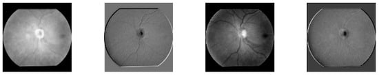
Figure 1.
Image processing process.
Figure 2 shows the workflow of the whole experiment. The process starts from the input image, goes through the selection of the neural network and optimization algorithm, carries out hyperparameter tuning and parameter training iteration, and finally classifies the image, and completes the whole classification process by confirming the classification accuracy.
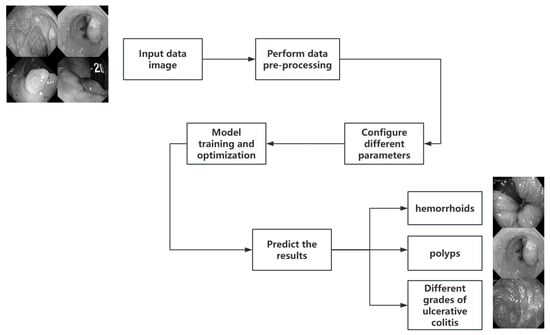
Figure 2.
Overall workflow.
3.2.1. Channel Rearrangement Mechanism
Channel rearrangement [34] is a method that facilitates the exchange of information between different channels by rearranging the channels of a feature map. It improves the representation capability by disrupting the channel order of the feature map in a convolutional operation, enabling the network to better learn the feature complementarities across channels.
Suppose the size of the input feature map is ; B represents batch size, C represents channels, and H and W represent the height and width of the image.
The steps of the channel rearrangement operation are as follows.
- (1)
- Divide the number of channels of the input feature map into G groups, each containing channels.
- (2)
- Rearrange the feature map into , the channels of each group are considered as independent dimensions.
- (3)
- Perform the transposition of the channel dimensions to obtain a new feature map .
- (4)
- Spread and output in the new order, enabling the exchange of information between channels. The formula representation is shown in Equation (11).
Suppose the input tensor is , denoting one sample with three channels of size 32 × 32. Divide the number of channels C = 3 into G = 3 groups. The number of channels in each group is shown in Equation (12).
Each group contains one channel. Divide the 3 input channels into 3 groups to obtain a new tensor, the dimensions of which are shown in Equation (13).
After grouping, the tensor has 3 groups with only 1 channel in each group, and the dimensions of each group are 1 × 32 × 32. Next, the order of the channels in these groups needs to be swapped. Since there is only 1 channel in each group, the effect of swapping is relatively simple here. It actually rearranges the order of each group in the channel dimension. By switching the channels within the group, a new tensor is obtained, as shown in Equation (14).
For G = 3, the effect of channel swapping may be that the first group becomes the original second group, the second group becomes the original third group, and the third group becomes the original first group. The final output tensor is still 1 × 3 × 32 × 32, but the order of the channels is disrupted. So the original tensor shape needs to be restored, i.e., to 1 × 3 × 32 × 32. It is worth noting, however, that although the shape has not changed, the order of the channels has been rearranged. After this operation, the model will learn the correlation relationship between different channels, thus enhancing the ability to model channel information.
In this way, the network is able to enhance the feature interaction between different groups without increasing the effort, thus improving the information flow.
3.2.2. SECA Attention Mechanism
The ECA module (Efficient Channel Attention) is a lightweight channel attention mechanism that automatically learns the importance of each channel by weighting the features of each channel. Unlike traditional channel attention methods, the ECA module captures the dependencies between channels through 1D convolution, thus reducing computation and improving efficiency.
The components of the ECA module are as follows.
(1) Global average pooling (GAP) is performed for each channel to obtain the global statistics of the channel. The pooling operation averages each channel over the spatial dimension to obtain a C-dimensional vector with the mathematical formulation shown in Equation (15).
denotes the value of channel c at position (h, w) in the feature map X, and is the average value of channel c.
(2) One-dimensional convolution calculates channel weights by passing the pooled feature y into a 1D convolution layer to get the attention weights of each channel. The size of the convolution kernel is typically 3, the step size is 1, and the padding is 1. After the convolution operation, the channel attention coefficient is obtained as shown in Equation (16).
denotes the activation function and Conv1D denotes the 1D convolution operation.
(3) Weighted feature plots represent that in the ECA module, the final channel attention coefficient a is broadcast onto the original input feature plot X and multiplied channel by channel, thus weighting the features of each channel. The final output feature map does the weighting of the channels, thus allowing the network to automatically focus on the more important channels. The mathematical formula for this step is shown in Equation (17).
is the channel attention coefficient obtained by 1D convolution, which is multiplied with X through the broadcast mechanism to obtain a weighted feature map.
In order to understand the working principle of the ECA module more intuitively, a flowchart is used to show its main computational process. Starting from the input feature map, the channel information is extracted through global average pooling, and then the channel weights are learned through 1D convolution and the activation function, and finally the weighted feature map is generated. The flowchart of the ECA module is shown in Figure 3.
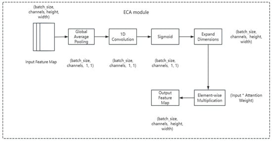
Figure 3.
ECA module flowchart.
SECA (Scaled ECA) is based on the design of the ECA module and introduces two additional adjustable hyperparameters γ and b, which can be used to scale and shift the attention weights. With these parameters, SECA can control the intensity of attention, thereby increasing or decreasing attention to a particular channel. The attention calculation method is different from the original ECA module. The SECA module scales and shifts the weights after convolution, and the calculation formula is shown in Equation (18).
is the channel importance of the convolutional output, controls the intensity of the attention, and b controls the offset of the attention. This allows you to be more flexible in adjusting the role of the attention mechanism rather than simply compressing it into the [0, 1] interval via sigmoid activation. The difference between the ECA and SECA modules is shown in Table 2.
Table 2.
Differences between ECA and SECA modules.
The SECA module is more flexible than the ECA module, and parameters γ and b allow the model to adjust the intensity of channel attention according to different task requirements. This is useful for some complex tasks, such as working with different types of images or different network architectures, where the model’s attention mechanism can be adapted to the characteristics of the data. In general, the SECA module adds a flexible adjustment mechanism while retaining the core structure of the original ECA module.
3.2.3. Activation Function and Architecture Optimization
In the original MobileNetV2, the activation function used was ReLU6, which is a variant of ReLU with restrictions, mainly used to stabilize the gradient in low-precision computational and quantization models, preventing the value from being too large or too small. However, the problem of “dead neurons” (i.e., some neurons always output zero during training, resulting in the disappearance of the gradient) still exists in ReLU6, especially when the network is deep, which affects the efficiency of the model training.
To solve this problem, replace the ReLU6 activation function with the LeakyReLU activation function. The LeakyReLU activation function is shown in Equation (19).
is a very small constant, usually taking the value of 0.01. LeakyReLU is able to maintain a small slope in the negative region, so that even if the neuron’s input is negative, the output will not be completely zero, thus avoiding the problem of “dead neurons” in ReLU. This allows the gradients in the network to flow better, improving the stability and efficiency of the training process. Figure 4 and Figure 5 show the internal modules of ESM and the structure of the network architecture.
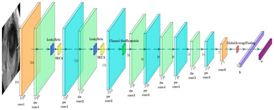
Figure 4.
ESM network architecture diagram.
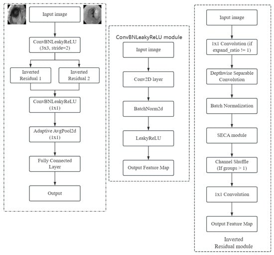
Figure 5.
ESM internal structure diagram.
The ESM network architecture and parameters are shown in Table 3.
Table 3.
ESM network architecture and parameter configuration.
4. Experimental Design and Analysis of Results
4.1. Experimental Dataset and Pre-Processing
The entire experimental code was written using the PyTorch lightning framework. The programming language is Python, Python language version is 3.10, the torch version is 2.0.1, the torch vision version is 0.15.0, the lightning version is 2.1.2, and the wandb version is 0.16.0.
The standard dataset CIFAR10 was used in the experiment, as well as image classification experiments in the medical field to test the performance and effectiveness of the RMA algorithm and the ESM network. There are three datasets involved in this experiment: CIFAR10 is a color image dataset containing different types of items and the image size is 32 × 32 in the experiment; the medical datasets used are the fundus glaucoma dataset [35] and the gastrointestinal disease dataset. The gastrointestinal disease dataset contains a total of eight classifications mainly consisting of different grades of hemorrhoids, polyps, and ulcerative colitis; the fundus glaucoma dataset mainly includes two categories, with and without glaucoma. The data volume, dataset division, and number of data classifications for the three datasets are shown in Table 4.
Table 4.
Data volume, dataset division, and number of data categories for the three datasets.
During the experiment, a center cropping operation is performed on the original picture. The images are randomly rotated 15 degrees, which helps to increase the diversity of the data and improve the generalization ability of the model. The image is enlarged to 1.25 times its original size, which is done to increase the diversity of the data while ensuring that the image is not distorted. The regularization process is carried out to standardize the pixel values of the image, so that it falls in a unified range, which is conducive to the training and convergence of the network. Taking an image in the fundus green-light dataset as an example, the image pre-processing process is shown in Figure 6.
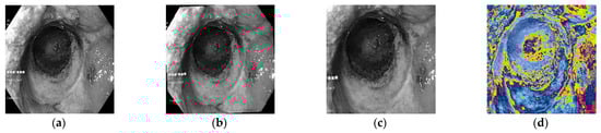
Figure 6.
Image pre-processing process. (a) Original drawing. (b) Randomly rotate 15°. (c) Cut and enlarge the center by 1.25 times. (d) Normalization.
During the training process, by comparing the accuracy and loss values, the performance of different optimization algorithms on the current task can be evaluated to find the most suitable optimization strategy.
Accuracy is a measure of the overall prediction accuracy of a classification model, defined as the ratio of the number of samples correctly predicted by the model to the total number of samples. Its formula is shown in Equation (20).
(true positive) represents the number of positive samples that are correctly predicted as positive classes; (true negative) is the number of negative samples that are correctly predicted as negative classes; (false positive) is the number of negative samples incorrectly predicted as a positive class; and (false negative) is expressed as the number of positive samples that are incorrectly predicted as negative classes.
The cross-entropy loss function is a measure of the difference between two probability distributions and is widely used in deep learning. For a given true distribution P and predictive distribution Q, the formula is shown in Equation (21).
represents the probability of the ground truth distribution, which is usually one-hot coding for classification tasks; is expressed as a prediction distribution (the probability of model output); and is expressed as the logarithm of the predicted probability of the real class, multiplied by the corresponding true probability, and summed to take a negative sign.
Such comparative experiments on pretreatment and optimization algorithms were used to guide the selection of the best data processing and optimization strategy in practical applications.
4.2. Experimental Setup
The RMA algorithm aims to quickly discover locally optimal solutions to enable optimal levels of test accuracy and loss values to enhance the performance of the optimization algorithm. In order to fully evaluate the performance of the RMA algorithm on different neural networks and to highlight the comparative results of the comparative experiments, extensive tests and studies were conducted on three datasets and neural network models. The CIFAR10, fundus glaucoma, and gastroenterology datasets were selected; all three datasets contain color RGB images. Two lightweight neural networks, MobileNetV2 and ShuffleNetV2, were chosen as the base models for training.
The specific steps during the experiment are as follows.
- (1)
- Optimization algorithms: This experiment covers five optimization algorithms, namely SGD, Adagrad, Adam, NAdam, and RMA algorithms, aiming at comparing the performance difference between them.
- (2)
- Batch size: The batch size used in each experiment is 32 to ensure the consistency and fairness of the experiment.
- (3)
- Statistical analysis and repeatability verification: To ensure the statistical reliability of the experimental results, we conducted 5 independent repeated experiments on all optimization algorithms and network combinations, recorded the classification accuracy and loss values of the test set, calculated the mean and standard deviation to evaluate stability, and presented the final results in the form of “accuracy (mean ± standard deviation)”(such as 92.73 ± 0.82%).
- (4)
- Hyperparameter selection method: For key hyperparameters in the RMA algorithm and ESM network (momentum term quantity M, scaling factor γ, and offset β of the SECA module), Optuna optimized with hyperparameters will be used for automated hyperparameter optimization. Set the search space (integers M ∈ [2, 5], γ ∈ [0.5, 2.0], and β ∈ [−0.5, 0.5]) with validation set accuracy as the optimization objective, and select the optimal parameter combination for performance.
- (5)
- Data pre-processing: Before conducting the experiments, necessary pre-processing of the data was carried out, including data normalization, standardization, data enhancement, and other operations to ensure the quality and consistency of the input data.
4.3. Experimental Results and Analysis
4.3.1. Application of RMA Algorithm on CIFAR10 Dataset
As for the selection of parameters, in this experiment, a total of three groups of different learning rates are involved, and a comparative analysis is carried out. In the experiment, the size of the learning rate should be determined in order to better determine the values of other hyperparameters. This is essential for the accuracy and reliability of the experiment. CIFAR10 dataset was selected for testing, the optimization algorithm was the Adam algorithm, and the epoch rounds were 30 rounds. The experimental results of different learning rates of CIFAR10 datasets in the test set are shown in Table 5.
Table 5.
Experimental results of CIFAR10 dataset with different learning rates.
From Table 5, it can be observed that there are differences in the classification performance of MobileNetV2, ShuffleNetV2, and ResNet50 under 30 rounds of training using the Adam optimizer with different learning rates. These results are only intended as a reference for performance testing and not as a final performance evaluation, as actual experiments usually require 100 rounds or more to draw more stable conclusions. The following is a specific analysis of the results.
With a learning rate of 0.01, the ShuffleNetV2 network has a higher loss, possibly due to the unstable gradient update caused by the larger learning rate. When the learning rate is 0.001, the performance of the MobileNetV2 network improves significantly, the accuracy rate reaches 70.48%, and the loss drops to 1.224, indicating that this is the best test learning rate. For the ShuffleNetV2 network, the accuracy rate also improves, reaching 65.39%, and the loss decreases to 1.61. Similarly, the ResNet50 network achieves its best results at this learning rate, with accuracy increasing to 72.43% and loss decreasing to 1.099. A learning rate of 0.0001 is too low, resulting in poor performance across all models. The accuracy of MobileNetV2, ShuffleNetV2, and ResNet50 networks drops to 40.77%, 40.76%, and 46.01%, respectively, with losses of 1.6988, 2.181, and 1.459, indicating that the training effect is not fully reflected at this rate.
The next experiment will test the performance of different algorithms on the CIFAR10 dataset in more depth, based on a learning rate of 0.001. The number of training rounds is expanded to 100 to fully tap the potential of each algorithm and ensure that the model can converge to a more stable state. By extending the training time, we hope to more comprehensively evaluate the performance of different optimization algorithms on MobileNetV2, ShuffleNetV2, and ResNet50. The exact values of the five optimization algorithms in the two neural networks are shown in Figure 7.
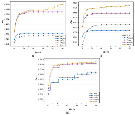
Figure 7.
Comparison of the accuracy effect of the three networks: (a) The accuracy values of the MobileNetV2 network. (b) The accuracy values of the ShuffleNetV2 network. (c) The accuracy values of the ResNet50 network.
On the test set, the accuracy rate and loss value of different optimization algorithms in the CIFAR10 dataset are shown in Table 6.
Table 6.
Accuracy and magnitude of loss values for different optimizers on CIFAR10 dataset.
4.3.2. Application of RMA Algorithm on Gastroenterology Dataset
The gastrointestinal disease dataset covers eight different classifications, including hemorrhoids, polyps, and ulcerative colitis with varying severity levels. Hemorrhoids are one of the most common diseases of the anus and rectum, affecting the quality of life of a large number of patients. Polyps are abnormal growths in the lining of the digestive tract that have the potential to become malignant and may develop into cancer. Ulcerative colitis is a complex inflammatory bowel disease that is classified into several severity levels, including mild, moderate, and severe. The objective of this dataset is to provide comprehensive coverage of these diseases and their variation characteristics, and to provide high-quality training data for relevant medical research and the development of intelligent diagnostic models.
In the experimental setup, the gastrointestinal disease dataset was used for training, aiming to explore the performance of different optimization algorithms on this specific dataset. During the training process, special attention was paid to the performance of the optimization algorithms in dealing with complex medical data, whether they can reach convergence quickly in extracting and classifying the features of different classes of diseases, and their ability to deal with difficult-to-distinguish classes. The accuracy values of the five optimization algorithms in the two neural networks are shown in Figure 8.
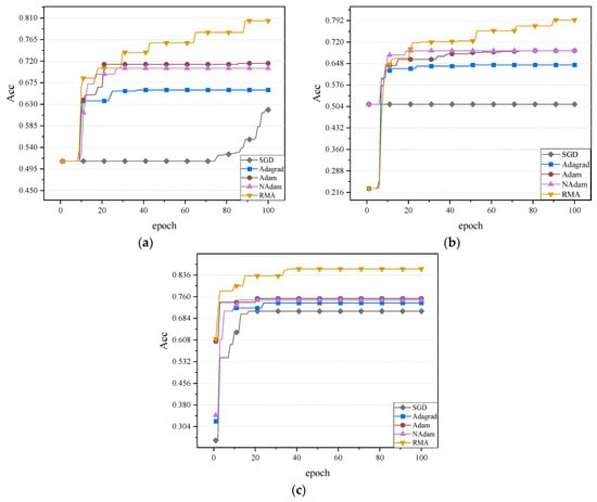
Figure 8.
Comparison of the accuracy effect of the three networks: (a) The accuracy values of the MobileNetV2 network. (b) The accuracy values of the ShuffleNetV2 network. (c) The accuracy values of the ResNet50 network.
The increase in classification accuracy and the decrease in loss value are important indicators of algorithm performance, and these data will provide a basis for further optimization of the model and algorithm. The magnitude of accuracy and loss values of different optimizers on the test set for the gastroenterology dataset are shown in Table 7.
Table 7.
Accuracy and magnitude of loss values for optimizers on the gastroenterology dataset.
It can be observed from Table 7 that there are significant differences in the performance of different optimization algorithms on gastrointestinal disease datasets, which is reflected in the classification accuracy and loss value indexes of MobileNetV2, ShuffleNetV2, and ResNet50 models. This effect is especially significant when the model reaches a stable state after 100 training cycles. This finding emphasizes the key role of optimization algorithms in the training of deep learning models and provides a valuable reference for subsequent research.
The RMA algorithm performs better than other optimization algorithms on both models. On the MobileNetV2 model, the classification accuracy of RMA reaches 83.60% with the lowest loss value of 0.741. The accuracy and loss performance are similar on the NAdam and Adam algorithms. With the ShuffleNetV2 model, RMA also performs well, with a classification accuracy of 81.60% and loss value of 0.808, which is better than other optimizers. On the ResNet50 model, RMA also performed well, with a classification accuracy of 84.94% and a loss value of 0.708, outperforming other optimizers.
Taking the ResNet50 model as an example, the confusion matrix of the RMA algorithm on the gastrointestinal disease dataset is shown in Figure 9.
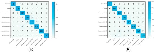
Figure 9.
Confusion matrix: (a) Confusion matrix under verification set. (b) Confusion matrix under test set.
In summary, the optimization ability of the RMA algorithm on complex medical datasets has been reflected. This shows that RMA algorithm has great potential in processing medical image data and improving the performance of deep learning models.
4.3.3. Application of the RMA Algorithm to the Fundus Glaucoma Dataset
The fundus glaucoma dataset mainly includes cases with and without glaucoma. Cases with glaucoma included fundus images of those who had already been diagnosed with glaucoma, while cases without glaucoma included healthy fundus images or images of patients who had not been diagnosed with glaucoma. The accuracy and loss values of five optimizers on the validation set on the neural network MobileNetV2, ShuffleNetV2, and ResNet50 are shown in Figure 10, Figure 11 and Figure 12.
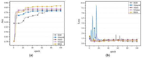
Figure 10.
Accuracy and loss values of five optimizers on neural network MobileNetV2: (a) Comparison of accuracy rates. (b) Comparison of loss values.
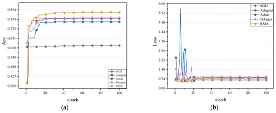
Figure 11.
Accuracy and loss values of five optimizers on neural network ShuffleNetV2: (a) Comparison of accuracy rates. (b) Comparison of loss values.
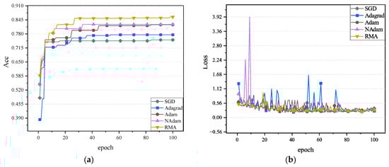
Figure 12.
Accuracy and loss values of five optimizers on neural network ResNet50: (a) Comparison of accuracy rates. (b) Comparison of loss values.
It can be observed in Figure 10, Figure 11 and Figure 12 that the RMA algorithm is superior to the other four algorithms in terms of accuracy. Secondly, the Adam algorithm and NAdam algorithm also perform better. In contrast, the performance of the SGD algorithm and Adagrad algorithm still needs to be further improved, especially the low accuracy on ShuffleNetV2. In terms of loss value, the SGD algorithm performs best. Future work will focus on further optimizing the loss-value performance of the RMA algorithm. In general, the RMA algorithm significantly improves the classification performance of the model and effectively reduces the loss value. The accuracy and loss values of the five optimizers on the fundus glaucoma dataset on the test set are shown in Table 8.
Table 8.
Accuracy and magnitude of loss values for the optimizers on the fundus glaucoma dataset.
The results of different optimization algorithms after 100 rounds of training can be observed from the data in Table 8. The classification accuracy and loss values of MobileNetV2, ShuffleNetV2, and ResNet50 models are compared. The RMA algorithm performed well on both models, with MobileNetV2 achieving an accuracy of 84.90% and a loss of 0.56, while ShuffleNetV2 achieved an accuracy of 83.60% and a loss of 0.621, while ResNet50 achieved an accuracy of 85.94% and a loss of 0.531. Although the RMA algorithm is superior to other algorithms in accuracy, its loss value is slightly higher than that of the SGD algorithm. Secondly, the performance of Adam and NAdam is also prominent, especially on MobileNetV2, where the accuracy rate of NAdam is 81.26% and the loss value is 0.489. In general, the RMA algorithm significantly improves the classification performance of the model and effectively reduces the loss value, demonstrating its advantages in the optimization process.
Taking the ResNet50 model as an example, the confusion matrix of the RMA algorithm on the gastrointestinal disease dataset is shown in Figure 13.
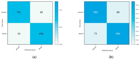
Figure 13.
Confusion matrix: (a) Confusion matrix under verification set. (b) Confusion matrix under test set.
The RMA algorithm demonstrates excellent optimization performance on complex medical imaging data, and its innovative region-weighting mechanism and multi-momentum term design significantly enhance the model’s feature learning ability. The experimental results show that the algorithm can effectively capture key region features with fractal characteristics in medical images, while maintaining more stable convergence while improving the classification accuracy of the model. This optimization method designed for the characteristics of medical images provides a new technological path for building high-performance medical diagnostic models, especially in early lesion recognition and fine-grained classification tasks, and demonstrates unique advantages.
4.3.4. Combination of RMA Algorithm and ESM Neural Network
To further enhance the network performance, the RMA algorithm is combined with the ESM network structure. The RMA algorithm strengthens the feature extraction capability for important regions by dynamically adjusting the feature attention strength in different regions. This algorithm works in conjunction with the channel attention mechanism of the SECA module and the feature reorganization mechanism of the Channel Shuffle module to achieve more efficient multi-scale feature expression. The combined network can capture global information as well as accurately recognize detailed features in key regions when dealing with complex scenes, thus significantly improving the performance of the model in diverse tasks.
After combining the RMA algorithm with the current network structure, a series of experiments are conducted to verify its effectiveness. The experimental results show that after the introduction of the RMA algorithm, the model demonstrates higher accuracy in processing multi-scale features, especially in the processing of complex backgrounds and detailed parts. By working in concert with the SECA and Channel Shuffle modules, the model is able to focus on important regions more effectively, significantly improving the recognition accuracy. In addition, the combined network outperforms the benchmark model without the RMA algorithm on different datasets, demonstrating greater adaptability and robustness. The accuracy effect graphs of the experimental results of the two datasets on the validation set are shown in Figure 14.
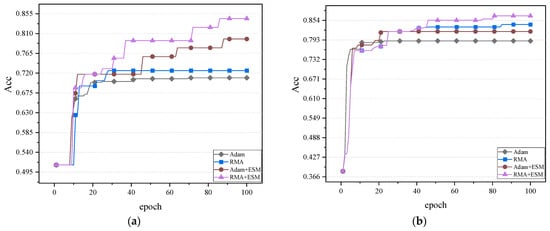
Figure 14.
Comparison of the accuracy effect of the two datasets: (a) Comparison of accuracy of gastrointestinal disease dataset. (b) Comparison of accuracy of fundus glaucoma dataset.
It can be observed from Figure 14 that the comparison of four combinations, including the Adam algorithm and the RMA algorithm, is conducted in combination with the ESM network, respectively. In the validation sets of different datasets, the combination effect of the RMA algorithm and ESM network is obviously better than the other three combination methods. Due to its innovative region-weighting mechanism, the RMA algorithm can dynamically identify key regions with diagnostic value in medical images, and combine multi-momentum term design to achieve more accurate gradient updates. At the same time, the ESM network effectively enhances the model’s ability to extract multi-scale medical features through its improved SECA attention module and channel recombination mechanism.
This indicates that the RMA algorithm combined with ESM network optimization has stronger advantages in improving model accuracy and reducing loss. This result shows that the optimization ability of RMA algorithm and the feature extraction and model generalization ability of the ESM network complement each other, and jointly promote model performance.
For the medical field, the effectiveness of this combination of optimization can not only improve the accuracy of disease diagnosis, but also provide more accurate model support for personalized medicine, thereby helping early diagnosis and disease prevention.
Table 9 shows the accuracy and loss values of the three neural networks on the test set of the gastrointestinal disease dataset.
Table 9.
Accuracy and loss values of three neural networks on test set of gastrointestinal disease.
By comparing the performance of the Adam and RMA optimization algorithms on MobileNetV2, ShuffleNetV2, ResNet50, and ESM networks, it can be found that the RMA algorithm exhibits a significant advantage over the Adam algorithm in terms of both accuracy rate and loss value. Specifically, in the MobileNetV2 model, the RMA algorithm resulted in an 11.2% increase in accuracy and a reduction in the loss value to 0.741, while the Adam algorithm had an accuracy of 72.40% and a loss value of 0.892.It performs the best among the five optimization algorithms.
In the ShuffleNetV2 model, the RMA algorithm achieved an accuracy of 81.60% with a loss value of 0.808, compared to the Adam algorithm with an accuracy of 70.40% and a loss value of 0.92 again achieving better results.
In the ResNet50 model, the RMA algorithm achieved an accuracy of 84.94% with a loss value of 0.708, compared to the Adam algorithm with an accuracy of 72.56% and a loss value of 0.824, again achieving better results.
In the ESM network, the RMA algorithm also performs well, with an accuracy of 87.30% and a loss value of 0.601, which is significantly superior compared to the Adam algorithm with an accuracy of 76.10% and a loss value of 0.71. Table 10 shows the accuracy and loss values of the three neural networks on the test set fundus glaucoma dataset.
Table 10.
Accuracy and loss values of three neural networks on test set of fundus glaucoma.
By comparing the performance of Adam and RMA optimization algorithms on MobileNetV2, ShuffleNetV2, ResNet50, and ESM network models on the fundus green-light dataset, it can be clearly seen that the RMA algorithm is significantly better than the Adam algorithm on all models. Specifically, in the MobileNetV2 model, the RMA algorithm achieves an accuracy of 84.90%, which is a 3.5% improvement compared to the 81.40% of the Adam algorithm. In terms of loss value, the RMA algorithm is 0.56, which is significantly lower compared to the 0.653 of the Adam algorithm.
In the ShuffleNetV2 model, the RMA algorithm has an accuracy of 83.60% and a loss value of 0.621, which is better than the Adam algorithm’s 80.82% accuracy and 0.834 loss value.
In the ResNet50 model, the RMA algorithm achieved an accuracy of 85.94% with a loss value of 0.521. It performs the best among the five optimization algorithms.
In the ESM network model, the RMA algorithm performs the most outstandingly, with an accuracy of 92.73%, which is improved by 8.53% compared to the 84.20% of the Adam algorithm. Also, the loss value is significantly reduced to 0.419, which is much lower than the 0.582 of the Adam algorithm.
Taking ResNet50 and ESM models as examples, the running times of Adam and RMA optimization algorithms are shown in Table 11.
Table 11.
The running time of the five optimization algorithms.
The experimental results combining the improved network and algorithm were compared with the accuracy of previous work on the glaucoma dataset and gastrointestinal disease dataset. The comparison results are shown in Table 12 and Table 13.
Table 12.
Comparison of accuracy on fundus glaucoma dataset.
Table 13.
Comparison of accuracy on gastrointestinal disease dataset.
In general, the RMA algorithm can effectively improve the classification accuracy of the model on the fundus glaucoma and gastrointestinal disease datasets, and significantly reduce the loss value, which further demonstrates its potential in medical image analysis, especially in improving the accuracy of early disease diagnosis.
5. Conclusions
Aiming at the limitations of traditional optimization algorithms in medical image analysis tasks, an RMA optimization algorithm based on a region-weighted mechanism and multi-momentum term design is proposed in this study, and an ESM neural network is constructed by combining them for an improved feature extraction module. The RMA optimization algorithm improves the stability and convergence efficiency of the optimization process by introducing the region-weighted mechanism and combining it with the multi-momentum design. On the basis of the traditional feature extraction module, the ESM neural network further improves the ability to capture the subtle features of medical images through the channel rearrangement mechanism. It is worth noting that the current method performs direct calculations based on the fractal features of the original image. In the future, the combination of adaptive contrast enhancement technology and fractal analysis can be explored to improve image quality while ensuring the preservation of key texture features. Future research can be carried out to further optimize the adaptability of the model, so that it can better process different modes of medical image data, and to explore the potential application of the RMA algorithm and ESM network in more medical fields, such as in tumor detection and pathological analysis. These improvements will help drive the widespread application of deep learning-based medical image analysis technology in clinical practice.
Author Contributions
Conceptualization, J.Y.; methodology, J.Y.; writing—original draft preparation, J.Y.; software, Y.S.; project administration, Y.S.; resources, Y.S.; data curation, W.Z.; writing—review and editing, H.S.; supervision, H.S.; formal analysis, H.S.; funding acquisition, Q.G. All authors have read and agreed to the published version of the manuscript.
Funding
This research was funded by Liaoning Provincial Department of Education Basic Research Project for Higher Education Institutions (General Project), Shenyang University of Technology, Research on Optimization Design of Wind Turbine Cone Angle Based on Fluid Physics Method (LJKZ0159); Basic Research Project of Liaoning Provincial Department of Education “Training and Application of Multimodal Deep Neural Network Models for Vertical Fields” Project Number: JYTMS20231160; Research on the Construction of a New Artificial Intelligence Technology and High Quality Education Service Supply System in the 14th Five Year Plan for Education Science in Liaoning Province, 2023-2025, Project Number: JG22DB488; “Chunhui Plan” of the Ministry of Education, Re-search on Optimization Model and Algorithm for Microgrid Energy Scheduling Based on Biological Behavior, Project No. 202200209; Shenyang Science and Technology Plan “Special Mission for Leech Breeding and Traditional Chinese Medicine Planting in Dengshibao Town, Faku Country”, Project No. 22-319-2-26 and Research on Compression Algorithm of Deep Neural Network Model for Personnel Re identification, Project number: 2024PY025.
Data Availability Statement
The original data presented in the study are openly available. The location of the Python code used in this paper is https://github.com/icecream1024/RMA-ESM (accessed on 6 May 2024). The website for the standard CIFAR10 dataset is https://www.cs.toronto.edu/~kriz/cifar.html (accessed on 6 May 2024). The website for the medical dataset is https://doi.org/10.1038/s41597-020-00622-y (accessed on 6 May 2024) and for the glaucoma dataset is https://www.kaggle.com/datasets/sabari50312/fundus-pytorch (accessed on 6 May 2024).
Conflicts of Interest
The authors declare no conflicts of interest.
References
- Gupta, A.; Dixit, M.; Mishra, V.K.; Singh, A.; Dayal, A. Brain tumor segmentation from MRI images using deep learning techniques. In International Advanced Computing Conference; Springer Nature: Cham, Switzerland, 2022; pp. 434–448. [Google Scholar]
- Tang, L.Y.W. Severity classification of ground-glass opacity via 2-D convolutional neural network and lung CT scans: A 3-day exploration. arXiv 2023, arXiv:2303.16904. [Google Scholar]
- Pandit, B.R.; Alsadoon, A.; Prasad, P.; Al Aloussi, S.; Rashid, T.A.; Alsadoon, O.H.; Jerew, O.D. Deep learning neural network for lung cancer classification: Enhanced optimization function. Multimed. Tools Appl. 2023, 82, 6605–6624. [Google Scholar] [CrossRef]
- Nanni, L.; Manfè, A.; Maguolo, G.; Lumini, A.; Brahnam, S. High performing ensemble of convolutional neural networks for insect pest image detection. Ecol. Inform. 2022, 67, 101515. [Google Scholar] [CrossRef]
- Zhou, T.; Huo, B.Q.; Lu, H.L.; Shi, H.B. Progress of residual neural network optimization algorithm for medical imaging disease diagnosis. Chin. J. Image Graph. 2020, 25, 2079–2092. [Google Scholar] [CrossRef]
- Kingma, D.P. Adam: A method for stochastic optimization. arXiv 2014, arXiv:1412.6980. [Google Scholar]
- Guan, L. AdaPlus: Integrating Nesterov momentum and precise stepsize adjustment on AdamW basis. In Proceedings of the ICASSP 2024–2024 IEEE International Conference on Acoustics, Speech and Signal Processing (ICASSP), Seoul, Republic of Korea, 14–19 April 2024; pp. 5210–5214. [Google Scholar]
- Dozat, T. Incorporating Nesterov Momentum into Adam. Available online: https://openreview.net/forum?id=OM0jvwB8jIp57ZJjtNEZ (accessed on 19 February 2024).
- Zhuang, J.; Tang, T.; Ding, Y.; Tatikonda, S.C.; Dvornek, N.; Papademetris, X.; Duncan, J. Adabelief optimizer: Adapting stepsizes by the belief in observed gradients. Adv. Neural Inf. Process. Syst. 2020, 33, 18795–18806. [Google Scholar]
- Yun, J. StochGradAdam: Accelerating Neural Networks Training with Stochastic Gradient Sampling. arXiv 2023, arXiv:2310.17042. [Google Scholar]
- Zhang, C.; Shao, Y.; Sun, H.; Xing, L.; Zhao, Q.; Zhang, L. The WuC-Adam algorithm based on joint improvement of Warmup and cosine annealing algorithms. Math. Biosci. Eng. 2024, 21, 1270–1285. [Google Scholar] [CrossRef]
- Sun, H.; Zhou, W.; Shao, Y.; Cui, J.; Xing, L.; Zhao, Q.; Zhang, L. A Linear Interpolation and Curvature-Controlled Gradient Optimization Strategy Based on Adam. Algorithms 2024, 17, 185. [Google Scholar] [CrossRef]
- Haase, D.; Amthor, M. Rethinking depthwise separable convolutions: How intra-kernel correlations lead to improved mobilenets. In Proceedings of the IEEE/CVF Conference on Computer Vision and Pattern Recognition, Seattle, WA, USA, 13–19 June 2020; pp. 14600–14609. [Google Scholar]
- Hoang, V.T.; Jo, K.H. Pydmobilenet: Improved version of mobilenets with pyramid depthwise separable convolution. arXiv 2018, arXiv:1811.07083. [Google Scholar]
- Qin, Z.; Zhang, Z.; Chen, X.; Wang, C.; Peng, Y. Fd-mobilenet: Improved mobilenet with a fast downsampling strategy. In Proceedings of the 25th IEEE International Conference on Image Processing (ICIP), Athens, Greece, 7–10 October 2018; pp. 1363–1367. [Google Scholar]
- Wang, H.; Zhu, W.; Dong, X.; Chen, Y.; Li, X.; Qiu, P.; Chen, X.; Vasa, K.V.; Xiong, Y.; Dumitrascu, O.M.; et al. Many-MobileNet: Multi-Model Augmentation for Robust Retinal Disease Classification. arXiv 2024, arXiv:2412.02825. [Google Scholar]
- Ahmadi, M.; Karimi, N.; Samavi, S. A lightweight deep learning pipeline with DRDA-Net and MobileNet for breast cancer classification. arXiv 2024, arXiv:2403.11135. [Google Scholar]
- Zhao, L.; Xu, X.; Li, J.; Zhao, Q. Application of deep-transfer learning in automatic glaucoma detection. J. Harbin Eng. Univ. 2023, 44, 673–678. [Google Scholar]
- Lv, P.; Wang, Y.; Wang, S.; Yu, X.; Wu, C. Optic disc detection based on visual saliency in fundus image. Chin. J. Image Graph. 2021, 26, 2293–2304. [Google Scholar]
- Borgli, H.; Thambawita, V.; Smedsrud, P.H.; Hicks, S.; Jha, D.; Eskeland, S.L.; Randel, K.R.; Pogorelov, K.; Lux, M.; Nguyen, D.T.D.; et al. HyperKvasir, a comprehensive multi-class image and video dataset for gastrointestinal endoscopy. Sci. Data 2020, 7, 283. [Google Scholar] [CrossRef] [PubMed]
- Yin, Y.; Guo, Y. Research on Glaucoma Diagnosis Method based on deep learning. Microprocessor 2021, 42, 41–46. [Google Scholar]
- Xu, J. Research on Retinal Multi-Disease Classification Based on Deep Learning. Master’s Thesis, Donghua University, Shanghai, China, 2023. Available online: https://link.cnki.net/doi/10.27012/d.cnki.gdhuu.2023.001227 (accessed on 6 May 2024).
- Xing, J.; He, W.; Zhang, S. Application of deep learning algorithms in cortical cataract screening. Artif. Intell. 2023, 6, 67–73. [Google Scholar]
- Wang, S.; Ke, Y.; Wang, G. Application of artificial intelligence in quality control of gastrointestinal. Chin. J. Oncol. 2021, 48, 1215–1219. [Google Scholar]
- Zhu, C.; Wang, D.; Hua, Y.; Zhang, G. Application and prospect of artificial intelligence in gastric diseases. J. Gastroenterol. Hepatol. 2022, 31, 451–453. [Google Scholar]
- Zhu, S.; Xu, C.; Zhou, X.; Liu, L.; Lin, J. Colorectal polyp segmentation in endoscopic images using DeepLabV3. Chin. J. Med. Phys. 2023, 40, 944–949. [Google Scholar]
- Liu, L.; Lin, J.; Zhu, S.; Gao, J.; Liu, X.; Xu, C.; Zhu, J. ResNet-based interpretable computer vision model in the endoscopic evaluation of internal hemorrhoids. Mod. Dig. Interv. Diagn. Treat. 2023, 28, 972–975+980. [Google Scholar]
- Gong, A. A study on construction of an eye disease classification and diagnosis model by utilizing resnet deep neural network. J. Med. Forum 2024, 45, 379–383. [Google Scholar]
- Huang, L.; Liu, M.; Wu, Y.; Xu, A.; Xiang, Y.; Zhou, Y.; Lin, H. Prevention and telemedicine of eye disease based on deep learning and smart phones. J. Ophthalmol. 2022, 37, 230–237. [Google Scholar]
- Aziz, A.; Tezel, N.S.; Kaçmaz, S.; Attallah, Y. Early Diabetic Retinopathy Detection from OCT Images Using Multifractal Analysis and Multi-Layer Perceptron Classification. Diagnostics 2025, 15, 1616. [Google Scholar] [CrossRef]
- Yang, L.; Zhang, M.; Cheng, J.; Zhang, T.; Lu, F. Retina images classification based on 2D empirical mode decomposition and multifractal analysis. Heliyon 2024, 10, e27391. [Google Scholar] [CrossRef]
- Mahapatra, K. Fractal Dimension and Entropy Analysis of Medical Images for KNN-Based Disease Classification. Baghdad Sci. J. 2025, 22, 1354–1365. [Google Scholar]
- Sandler, M.; Howard, A.; Zhu, M.; Zhmoginov, A.; Chen, L. Mobilenetv2: Inverted residuals and linear bottlenecks. In Proceedings of the IEEE Conference on Computer Vision and Pattern Recognition, Salt Lake City, UT, USA, 18–22 June 2018; pp. 4510–4520. [Google Scholar]
- Ma, N.; Zhang, X.; Zheng, H.T.; Sun, J. Shufflenet v2: Practical guidelines for efficient cnn architecture design. In Proceedings of the European Conference on Computer Vision(ECCV), Munich, Germany, 8–14 September 2018; pp. 116–131. [Google Scholar]
- Kiefer, R.; Abid, M.; Ardali, M.R.; Steen, J.; Amjadian, E. Automated Fundus Image Standardization Using a Dynamic Global Foreground Threshold Algorithm. In Proceedings of the 8th International Conference on Image, Vision and Computing (ICIVC), Dalian, China, 27–29 July 2023; pp. 460–465. [Google Scholar]
- Hu, J.; Shen, L.; Sun, G. Squeeze-and-excitation networks. In Proceedings of the IEEE Conference on Computer Vision and Pattern Recognition, Salt Lake City, UT, USA, 18–22 June 2018; pp. 7132–7141. [Google Scholar]
- Woo, S.; Park, J.; Lee, J.Y.; Kweon, I.S. Cbam: Convolutional block attention module. In Proceedings of the European Conference on Computer Vision (ECCV), Munich, Germany, 8–14 September 2018; pp. 3–19. [Google Scholar]
- He, A.; Li, T.; Li, N.; Wang, K.; Fu, H. CABNet: Category attention block for imbalanced diabetic retinopathy grading. IEEE Trans. Med. Imaging 2020, 40, 143–153. [Google Scholar] [CrossRef]
- Cao, Y.; Xu, J.; Lin, S.; Wei, F.; Hu, H. Gcnet: Non-local networks meet squeeze-excitation networks and beyond. In Proceedings of the IEEE/CVF International Conference on Computer Vision Workshops, Seoul, Republic of Korea, 27 October–2 November 2019. [Google Scholar]
- Chakraborty, S.; Roy, A.; Pramanik, P.; Valenkova, D.; Sarkar, R. A Dual Attention-aided DenseNet-121 for Classification of Glaucoma from Fundus Images. In Proceedings of the 13th Mediterranean Conference on Embedded Computing (MECO), Budva, Montenegro, 11–14 June 2024; pp. 1–4. [Google Scholar]
- Gómez-Valverde, J.J.; Antón, A.; Fatti, G.; Liefers, B.; Herranz, A.; Santos, A.; Sánchez, C.I.; Ledesma-Carbayo, M.J. Automatic glaucoma classification using color fundus images based on convolutional neural networks and transfer learning. Biomed. Opt. Express 2019, 10, 892–913. [Google Scholar] [CrossRef]
- Alayón, S.; Hernández, J.; Fumero, F.J.; Sigut, J.F.; Díaz-Alemán, T. Comparison of the performance of convolutional neural networks and vision transformer-based systems for automated glaucoma detection with eye fundus images. Appl. Sci. 2023, 13, 12722. [Google Scholar] [CrossRef]
- Verma, R.; Shrinivasan, L.; Hiremath, B. Machine learning classifiers for detection of glaucoma. IAES Int. J. Artif. Intell. 2023, 12, 806. [Google Scholar] [CrossRef]
- Min, M.; Su, S.; He, W.; Bi, Y.; Ma, Z.; Liu, Y. Computer-aided diagnosis of colorectal polyps using linked color imaging colonoscopy to predict histology. Sci. Rep. 2019, 9, 2881. [Google Scholar] [CrossRef]
- Alhajlah, M.; Noor, M.N.; Nazir, M.; Mahmood, A.; Ashraf, I.; Karamat, T. Gastrointestinal diseases classification using deep transfer learning and features optimization. Comput. Mater. Contin. 2023, 75, 2227–2245. [Google Scholar] [CrossRef]
- Margapuri, V. Diagnosis and Severity Assessment of Ulcerative Colitis using Self Supervised Learning. arXiv 2024, arXiv:2412.07806. [Google Scholar]
- Ahlawat, V.; Sharma, R. Optimizing Gastrointestinal Diagnostics: A CNN-Based Model for VCE Image Classification. arXiv 2024, arXiv:2411.01652. [Google Scholar]
- Das, A.; Singh, A.; Prakash, S. CapsuleNet: A Deep Learning Model To Classify GI Diseases Using EfficientNet-b7. arXiv 2024, arXiv:2410.19151. [Google Scholar]
Disclaimer/Publisher’s Note: The statements, opinions and data contained in all publications are solely those of the individual author(s) and contributor(s) and not of MDPI and/or the editor(s). MDPI and/or the editor(s) disclaim responsibility for any injury to people or property resulting from any ideas, methods, instructions or products referred to in the content. |
© 2025 by the authors. Licensee MDPI, Basel, Switzerland. This article is an open access article distributed under the terms and conditions of the Creative Commons Attribution (CC BY) license (https://creativecommons.org/licenses/by/4.0/).