Article

An Eighth-Order Numerical Method for Spatial Variable-Coefficient Time-Fractional Convection–Diffusion–Reaction Equations

1
School of Mathematical Sciences, Xinjiang Normal University, Urumqi 830017, China
2
College of Big Data Statistics, Guizhou University of Finance and Economics, Guiyang 550025, China
3
School of Mathematics and Statistics, Henan University of Technology, Zhengzhou 450001, China
*
Author to whom correspondence should be addressed.
Fractal Fract. 2025, 9(7), 451; https://doi.org/10.3390/fractalfract9070451
Submission received: 18 June 2025 / Revised: 4 July 2025 / Accepted: 7 July 2025 / Published: 9 July 2025
(This article belongs to the Section Numerical and Computational Methods)

Abstract

In this paper, we propose a high-order compact difference scheme for a class of time-fractional convection–diffusion–reaction equations (CDREs) with variable coefficients. Using the Lagrange polynomial interpolation formula for the time-fractional derivative and a compact finite difference approximation for the spatial derivative, we establish an unconditionally stable compact difference method. The stability and convergence properties of the method are rigorously analyzed using the Fourier method. The convergence order of our discrete scheme is O ( τ 4 α + h 8 ) , where τ and h represent the time step size and space step size, respectively. This work contributes to providing a better understanding of the dependability of the method by thoroughly examining convergence and conducting an error analysis. Numerical examples demonstrate the applicability, accuracy, and efficiency of the suggested technique, supplemented by comparisons with previous research.

1. Introduction

In the realm of contemporary scientific research and engineering applications, mathematical models are indispensable, with partial differential equations serving as a cornerstone. These equations are capable of effectively capturing the essential characteristics of dynamic behaviors in various systems, ranging from natural phenomena to engineering optimization. However, as the complexity of research subjects continues to grow, traditional integer-order partial differential equations are increasingly insufficient. This limitation has driven researchers to explore new mathematical frameworks to meet these challenges.
Fractional calculus has emerged as a promising solution to address these limitations. Fractional differential equations, by incorporating fractional-order derivatives, can naturally describe systems with memory effects, non-local characteristics, and complex dynamics. This makes them a more flexible tool for modeling. Among the various fractional models, fractional CDREs have garnered significant attention due to their wide applicability across multiple fields. These equations are capable of describing the transport of substances in complex media and effectively characterizing reaction kinetics. This makes them highly valuable in areas such as environmental science [1,2], materials science [3,4], and biomedical engineering [5,6].
Nevertheless, solving fractional CDREs presents formidable challenges. The non-local nature of fractional derivatives, combined with potential nonlinear terms and variable coefficients in the equations, renders traditional numerical methods largely inadequate for efficiently solving these equations. Among the numerical methods for constant-coefficient cases, one can refer to the adaptive moving mesh method [7], finite element method [8,9,10], finite volume method [11], and finite difference method [12,13]. In contrast, the more practically significant variable-coefficient cases have received relatively little attention. The presence of variable coefficients complicates the physical properties of the equations and poses greater difficulties for the design and analysis of numerical methods. In recent years, scholars have made significant strides in addressing these challenges. In 2021, Li and Wang [14] developed numerical methods for time-fractional CDREs. They utilized finite differences for the Caputo fractional derivative and the local discontinuous Galerkin method for the spatial derivative. In 2022, Ngondiep [15] introduced an advanced two-level fourth-order numerical scheme designed for time-fractional CDREs with variable coefficients. This scheme demonstrated unconditional stability and achieved a convergence rate of O ( τ 2 α 2 + h 4 ) . In 2023, Roul and Rohil [16] introduced a numerical method for multiterm time-fractional CDREs. It employs a graded mesh for the Liouville–Caputo fractional derivative and a compact finite difference method for spatial derivatives. Additionally, Hosseini et al. [17] proposed a meshless Generalized Finite Difference Method for nonlinear fractional CDREs. This approach leverages Taylor series and Moving Least Squares for spatial derivatives, ensuring reliability across complex domains. In 2024, Priyadarshana and Mohapatra [18] devised a numerical algorithm for 2D time-delayed parabolic CDREs. It utilizes an operator-splitting method and an upwind scheme on a Shishkin mesh. The Thomas algorithm is applied for computation efficiency, achieving first-order accuracy. Furthermore, Kumar et al. [19] presented a weak Galerkin finite-element method for singularly perturbed CDREs. This approach ensures higher-order convergence rates and is applicable to various polygonal mesh types, achieving O ( h k ) in the triple-bar norm and O ( h k + 1 ) in the L 2 norm, where k represents the highest degree of the polynomials employed. In 2025, Liu et al. [20] proposed a high-order compact finite difference method for CDREs with variable exponents and coefficients. They used a space–time transformation and interpolation quadrature rule to handle the complexities. The aforementioned research results provide reliable references for numerical methods of fractional differential equations, but the convergence rates in both the time and space directions need further improvement. Inspired by the above research, this paper builds upon the studies of previous scholars and enhances the convergence rates of the algorithm in both the time and space directions, with convergence of the 4 α order in time and the eighth order in space.
In the present work, we consider more general time-fractional CDREs with variable coefficients in order to better model complex physical phenomena [21].
D t α 0 C v ( x , t ) = d 2 v x 2 ( x , t ) p 1 ( x ) v x ( x , t ) + p 2 ( x ) v ( x , t ) + f ( x , t ) , v ( 0 , t ) = φ 1 ( t ) , v ( L , t ) = φ 2 ( t ) , v ( x , 0 ) = φ 3 ( x ) ,
where ( x , t ) ( 0 , L ) × ( 0 , T ] , d is the constant diffusion coefficient, p 1 and p 2 are variable coefficients dependent on x, and f ( x , t ) represents external influences. The boundary conditions are φ 1 ( t ) at x = 0 and φ 2 ( t ) at x = L , and the initial condition is φ 3 ( x ) . All functions are assumed smooth enough to ensure the validity of the analysis. The Caputo fractional derivative D t α 0 C is defined as
D t α 0 C u ( t ) = 1 Γ ( 1 α ) 0 t u ( s ) ( t s ) α d s , 0 < α < 1 .
To address the complexities of solving variable-coefficient time-fractional CDREs, this paper presents a novel numerical approach. This approach leverages the Lagrange polynomial interpolation formula for the time-fractional derivative and a compact finite difference approximation for the spatial derivative. This method not only achieves unconditional stability but also attains convergence rates of the 4 α order in time and the eighth order in space, as rigorously analyzed through the Fourier method. By effectively addressing the challenges posed by variable coefficients, the proposed scheme significantly enhances numerical accuracy while maintaining computational efficiency. Three numerical experiments further validate the theoretical analysis, demonstrating superior performance compared to existing methods. This work thus offers a robust and efficient solution strategy for time-fractional CDREs, providing valuable support for modeling and analyzing complex systems in various fields.
This paper is organized as follows: Section 2 introduces the necessary mathematical notations and preliminary lemmas that form the foundation for developing our high-order compact finite difference scheme; Section 3 is dedicated to analyzing the stability and convergence properties of the proposed methods; Section 4 presents three numerical experiments that illustrate the practical application and effectiveness of our approach; and we conclude this paper with a summary of our findings and potential directions for future research in Section 5.

2. Construction of Full Discrete Scheme

To facilitate the analysis of Equation (1), we apply a series of transformations. These transformations are designed to address the challenges associated with variable coefficients and to simplify the equation by converting it into a more tractable form. Initially, we assume that the coefficient p 1 ( x ) is differentiable on the interval [ 0 , L ] and define the following notations:
u ( x , t ) = k ( x ) v ( x , t ) , g ( x , t ) = k ( x ) f ( x , t ) , k ( x ) = exp 1 2 d 0 x p 1 ( s ) d s , q ( x ) = p 2 ( x ) + 1 2 d p 1 d x p 1 2 2 d .
By addressing these complexities, Equation (1) is transformed into a more tractable form:
D t α 0 C u ( x , t ) = d 2 u x 2 ( x , t ) + q ( x ) u ( x , t ) + g ( x , t ) , x ( 0 , L ) , t ( 0 , T ] , u ( 0 , t ) = ϕ 1 ( t ) , u ( L , t ) = ϕ 2 ( t ) , t [ 0 , T ] , u ( x , 0 ) = ϕ 3 ( x ) , x [ 0 , L ] ,
where ϕ 1 ( t ) , ϕ 2 ( t ) , and ϕ 3 ( x ) are assumed to be sufficiently smooth. Clearly, v ( x , t ) is a solution of Equation (1) if and only if u ( x , t ) satisfies Equation (2). Consequently, the remainder of our study is dedicated to Equation (2).
To construct a high-precision compact finite difference scheme for Equation (2), we define M and N as the numbers of spatial and temporal subdivisions, respectively, and h = L M and τ = T N as the spatial and temporal step sizes. Let [ M ] = { 1 , 2 , , M } . We define u j n = u ( x j , t n ) and g j n = g ( x j , t n ) , where x j and t n are the spatial and temporal grid points. The difference operators are defined as follows:
δ x 2 u j = u j + 1 2 u j + u j 1 , L = 1 h 2 1 + 1 560 δ x 6 1 δ x 2 1 1 12 δ x 2 + 1 90 δ x 4 .
Here, we introduce several lemmas that are employed in the subsequent construction of the finite difference scheme.
Lemma 1
([22]). For the difference operator L , it holds that u x x ( x j , t n ) = L u j n + O ( h 8 ) .
Lemma 2
([23]). The discretized form of the Caputo derivative on a uniform mesh is given by
D t α 0 C u j n = 1 Γ ( 1 α ) [ t 0 t 1 ( t n s ) α u ( s ) d s + t 1 t 2 ( t n s ) α u ( s ) d s + k = 3 n t k 1 t k ( t n s ) α u ( s ) d s ] = 1 Γ ( 2 α ) k = 0 n λ k u j n k + O ( τ 4 α ) .
Here, the coefficients λ k are consistent with those reported in Reference [23].
Lemma 3
([23]). Let λ k be defined as τ α ψ k . The coefficients ψ k exhibit the following properties:
(i) 
For n 3 and any α in the interval ( 0 , 1 ) :
(i-1) 
ψ 0 is calculated as 1 3 + 1 2 α + 1 ( 2 α ) ( 3 α ) , and it falls within the range 1 , 11 6 .
(i-2) 
ψ 2 is positive.
(i-3) 
ψ k is negative for k 1 and k 2 .
(ii) 
For any order α ( 0 , 1 ) and for all n, the sum of coefficients equals zero, i.e., k = 0 n ψ k = 0 .
Now, using Lemmas 1 and 2, Equation (2) can be rewritten as
1 Γ ( 2 α ) k = 0 n λ k u j n k = d L u j n + q j u j n + g j n + O ( τ 4 α + h 8 ) .
By denoting U j n as the numerical estimate of u j n and omitting the truncation errors O ( τ 4 α + h 8 ) in Equation (3), we obtain
1 Γ ( 2 α ) k = 0 n λ k U j n k = d L U j n + q j U j n + g j n .
By multiplying both sides of Equation (4) by 1 + 1 560 δ x 6 and introducing the parameters μ = 1 Γ ( 2 α ) and θ = d h 2 , we obtain the final discrete formulation
μ λ 0 560 q j 560 θ 90 U j + 3 n + 3 μ λ 0 280 + 3 q j 280 + 3 θ 20 U j + 2 n + 3 μ λ 0 112 3 q j 112 3 θ 2 U j + 1 n + 27 μ λ 0 28 27 q j 28 + 49 θ 18 U j n + 3 μ λ 0 112 3 q j 112 3 θ 2 U j 1 n + 3 μ λ 0 280 + 3 q j 280 + 3 θ 20 U j 2 n + μ λ 0 560 q j 560 θ 90 U j 3 n = + 1 560 g j + 3 n 3 280 g j + 2 n + 3 112 g j + 1 n + 27 28 g j n + 3 112 g j 1 n 3 280 g j 2 n + 1 560 g j 3 n μ k = 1 n λ k ( 1 560 U j + 3 n k 3 280 U j + 2 n k + 3 112 U j + 1 n k + 27 28 U j n k + 3 112 U j 1 n k 3 280 U j 2 n k + 1 560 U j 3 n k ) ,
with the initial and boundary conditions
U j 0 = ϕ ˜ 3 ( x j ) , and U 0 n = ϕ ˜ 1 ( t n ) = ϕ ˜ 1 n and U M n = ϕ ˜ 2 ( t n ) = ϕ ˜ 2 n .
For the computation of ghost-point values, we utilize the extrapolation formulas presented below:
U 2 k = 36 U 0 k 168 U 1 k + 378 U 2 k 504 U 3 k + 420 U 4 k 216 U 5 k + 63 U 6 k 8 U 7 k + O ( h 8 ) , U 1 k = 8 U 0 k 28 U 1 k + 56 U 2 k 70 U 3 k + 56 U 4 k 28 U 5 k + 8 U 6 k U 7 k + O ( h 8 ) , U M + 1 k = 8 U M k 28 U M 1 k + 56 U M 2 k 70 U M 3 k + 56 U M 4 k 28 U M 5 k + 8 U M 6 k U M 7 k + O ( h 8 ) , U M + 2 k = 36 U M k 168 U M 1 k + 378 U M 2 k 504 U M 3 k + 420 U M 4 k 216 U M 5 k + 63 U M 6 k 8 U M 7 k + O ( h 8 ) .

3. Stability and Convergence Analyses

In this section, we conduct a comprehensive theoretical analysis to establish the stability and convergence of the proposed numerical method for solving time-fractional CDREs with variable coefficients.

3.1. Stability Analysis

In this subsection, let U ^ j n represent the approximate solution of Equation (5). We define the error term as
ε j n = U ^ j n U j n , j [ M 1 ] , n [ N ] .
Consequently, we have
μ λ 0 560 q j 560 θ 90 ε j + 3 n + 3 μ λ 0 280 + 3 q j 280 + 3 θ 20 ε j + 2 n + 3 μ λ 0 112 3 q j 112 3 θ 2 ε j + 1 n + 27 μ λ 0 28 27 q j 28 + 49 θ 18 ε j n + 3 μ λ 0 112 3 q j 112 3 θ 2 ε j 1 n + 3 μ λ 0 280 + 3 q j 280 + 3 θ 20 ε j 2 n + μ λ 0 560 q j 560 θ 90 ε j 3 n = μ k = 1 n λ k ( 1 560 ε j + 3 n k 3 280 ε j + 2 n k + 3 112 ε j + 1 n k + 27 28 ε j n k + 3 112 ε j 1 n k 3 280 ε j 2 n k + 1 560 ε j 3 n k ) .
The Fourier series representation of ε n ( x ) and its associated coefficients are given by
ε n ( x ) = l = ξ n ( l ) e i β x , where ξ n ( l ) = 1 L 0 L ε n ( x ) e i β x d x , β = 2 π l L and i = 1 .
By leveraging the definition of the L 2 norm and invoking Parseval’s theorem, we derive
ε n 2 = h i = 1 M 1 | ε i n | 2 = 0 L | ε i n | 2 d x and 0 L | ε n ( x ) | 2 d x = L l = | ξ n ( l ) | 2 ,
and, thus, we have
ε n 2 = L l = | ξ n ( l ) | 2 .
We make the Fourier series assumption for ε j n = ξ n e i β j h , and we substitute it into Equation (6). After simplification, we obtain
ξ n [ μ λ 0 280 q j 280 θ 45 cos ( 3 β h ) + 3 μ λ 0 140 + 3 q j 140 + 3 θ 10 cos ( 2 β h ) + 3 μ λ 0 56 3 q j 56 3 θ cos ( β h ) + 27 μ λ 0 28 27 q j 28 + 49 θ 18 ] = μ k = 1 n λ k 1 280 cos ( 3 β h ) 3 140 cos ( 2 β h ) + 3 56 cos ( β h ) + 27 28 ξ n k .
From Equation (8), it follows that ξ n can be written as
ξ n = k = 1 n μ λ k B 1 ( μ λ 0 q j ) B 1 + θ B 2 ξ n k ,
where B 1 and B 2 are defined as follows:
B 1 = 1 70 cos 3 ( β h ) 3 cos 2 ( β h ) + 3 cos ( β h ) + 69 , B 2 = 4 45 cos 3 ( β h ) 27 4 cos 2 ( β h ) + 132 4 cos ( β h ) 109 4 .
We use C to represent various positive, bounded constants that may differ from one case to another.
Theorem 1.
The numerical scheme given by Equation (5) is unconditionally stable for α ( 0 , 1 ) .
Proof. 
First, we apply mathematical induction to prove that
| ξ n | C | ξ 0 | , n [ N ] .
When n = 1 , according to Equation (9), we have
| ξ 1 | = | μ λ 1 B 1 ( μ λ 0 q j ) B 1 + θ B 2 ξ 0 | | μ λ 0 B 1 ( μ λ 0 q j ) B 1 + θ B 2 | | ξ 0 | ,
where λ 1 = λ 0 (refer to Kumari et al. [23] for details). Given that
μ = 1 Γ ( 2 α ) , θ = d h 2 , B 1 > 0 , B 2 0 ,
and that the function
q ( x ) = p 2 ( x ) + 1 2 d p 1 d x p 1 2 2 d ,
is bounded, we have
| ξ 1 | C | ξ 0 | .
Next, we assume that the inequality
| ξ n | C | ξ 0 |
holds for n = 2 , 3 , , N 1 .
When n = N , according to Equation (9) and Lemma 3, we have
| ξ N | = | k = 1 N μ λ k B 1 ( μ λ 0 q j ) B 1 + θ B 2 ξ N k | k = 1 N | μ λ k B 1 ( μ λ 0 q j ) B 1 + θ B 2 | | ξ N k | k = 1 N | ψ k | | μ τ α B 1 ( μ τ α ψ 0 q j ) B 1 + θ B 2 | C | ξ 0 | C ( ψ 0 + 2 ψ 2 ) | ξ 0 | C | ξ 0 | .
By Equations (7) and (11), we obtain
ε n 2 = L l = | ξ n ( l ) | 2 L l = C 2 | ξ 0 ( l ) | 2 = C 2 ε 0 2 .
Therefore, the numerical scheme given by Equation (5) is unconditionally stable. □

3.2. Convergence Analysis

In this subsection, we discuss the convergence of Equation (5). In a similar manner, let
E j n = u j n U j n , j [ M 1 ] , n [ N ] .
By subtracting Equation (4) from Equation (3) and noting that E j 0 = 0 , we can establish the following:
μ λ 0 560 q j 560 θ 90 E j + 3 n + 3 μ λ 0 280 + 3 q j 280 + 3 θ 20 E j + 2 n + 3 μ λ 0 112 3 q j 112 3 θ 2 E j + 1 n + 27 μ λ 0 28 27 q j 28 + 49 θ 18 E j n + 3 μ λ 0 112 3 q j 112 3 θ 2 E j 1 n + 3 μ λ 0 280 + 3 q j 280 + 3 θ 20 E j 2 n + μ λ 0 560 q j 560 θ 90 E j 3 n = + 1 560 R j + 3 n 3 280 R j + 2 n + 3 112 R j + 1 n + 27 28 R j n + 3 112 R j 1 n 3 280 R j 2 n + 1 560 R j 3 n μ k = 1 n 1 λ k ( 1 560 E j + 3 n k 3 280 E j + 2 n k + 3 112 E j + 1 n k + 27 28 E j n k + 3 112 E j 1 n k 3 280 E j 2 n k + 1 560 E j 3 n k )
where R j n = O ( τ 4 α + h 8 ) .
Similarly to the stability analysis, we define the grid functions E n ( x ) and R n ( x ) :
E n ( x ) = l = e n ( l ) e i β x , where e n ( l ) = 1 L 0 L E n ( x ) e i β x d x , β = 2 π l L and i = 1 , R n ( x ) = l = r n ( l ) e i β x , where r n ( l ) = 1 L 0 L R n ( x ) e i β x d x , β = 2 π l L and i = 1 .
Assuming that E j n = e n e i β j h and R j n = r n e i β j h and subtracting them from Equation (12), we derive
e n [ μ λ 0 280 q j 280 θ 45 cos ( 3 β h ) + 3 μ λ 0 140 + 3 q j 140 + 3 θ 10 cos ( 2 β h ) + 3 μ λ 0 56 3 q j 56 3 θ cos ( β h ) + 27 μ λ 0 28 27 q j 28 + 49 θ 18 ] = μ k = 1 n 1 λ k 1 280 cos ( 3 β h ) 3 140 cos ( 2 β h ) + 3 56 cos ( β h ) + 27 28 e n k + 1 280 cos ( 3 β h ) 3 140 cos ( 2 β h ) + 3 56 cos ( β h ) + 27 28 r n .
It follows that
e n = k = 1 n 1 μ λ k B 1 ( μ λ 0 q j ) B 1 + θ B 2 e n k + μ λ k B 1 ( μ λ 0 q j ) B 1 + θ B 2 r n .
In preparation for the proof of Theorem 2, we first introduce some necessary definitions:
E n 2 = h j = 1 M 1 | E j n | 2 = L l = | e n ( l ) | 2 ,
R n 2 = h j = 1 M 1 | R j n | 2 = L l = | r n ( l ) | 2 .
Theorem 2.
The numerical scheme given by Equation (5) converges with order O ( τ 4 α + h 8 ) .
Proof. 
We begin by employing mathematical induction to demonstrate the existence of a positive constant C such that the following inequality holds for all n [ N ] :
| e n | C | r 1 | .
Since R j n = O ( τ 4 α + h 8 ) , by Equation (15), we can assert the existence of a positive constant C n for each n [ N ] such that
| r n | C n | r 1 | .
When n = 1 , according to Equation (13), we obtain
| e 1 | = | μ λ 1 B 1 ( μ λ 0 q j ) B 1 + θ B 2 r 1 | | μ λ 0 B 1 ( μ λ 0 q j ) B 1 + θ B 2 | | r 1 | ,
and, similar to Equation (10), we can derive
| e 1 | C 1 | r 1 | .
Now, we assume that the inequality
| e n | C n | r 1 |
holds for n = 2 , 3 , , N 1 .
We define C as the maximum value among the constants { C 1 , C 2 , , C N } .
When n = N , according to Equation (13) and Lemma 3, we derive
| e N | = | k = 1 N 1 μ λ k B 1 ( μ λ 0 q j ) B 1 + θ B 2 e N k + B 1 ( μ λ 0 q j ) B 1 + θ B 2 r N | k = 1 N 1 | μ λ k B 1 ( μ λ 0 q j ) B 1 + θ B 2 | | e N k | + | B 1 ( μ λ 0 q j ) B 1 + θ B 2 | | r N | k = 1 N 1 | μ λ k B 1 ( μ λ 0 q j ) B 1 + θ B 2 | C N k | r 1 | + | B 1 ( μ λ 0 q j ) B 1 + θ B 2 | C N | r 1 | C | μ τ α B 1 ( μ τ α ψ 0 q j ) B 1 + θ B 2 | ( ψ 0 + 2 ψ 2 ) | r 1 | + C | B 1 ( μ τ α ψ 0 q j ) B 1 + θ B 2 | | r 1 | C ( 1 + ψ 0 + 2 ψ 2 ) | r 1 | C | r 1 | .
Then, by Equation (14) and (15), we obtain
E n 2 = L l = | e n ( l ) | 2 L l = C 2 | r 1 ( l ) | 2 = C 2 R 1 2 C 2 ( τ 4 α + h 8 ) 2 .
Therefore, the numerical scheme given by Equation (5) converges with order O ( τ 4 α + h 8 ) . □

4. Numerical Results

Our innovative high-order scheme for time-fractional CDREs with variable coefficients was rigorously validated through computational experiments, which revealed its convergence order and confirmed its effectiveness. All numerical experiments were conducted using MATLAB 2020b. The errors E 1 and E 2 were computed with mesh sizes h 1 and h 2 , respectively, and the errors and convergence rates were quantified as follows:
L - Error = max 1 n N | u n U n | , L - Rate = l o g ( E 1 / E 2 ) / l o g ( h 1 / h 2 ) .
To rigorously validate the accuracy and robustness of our proposed method, we compared its results against known analytical solutions under controlled conditions in Examples 1–3.
Example 1.
We examine Equation (2) in the domain [ 0 , 2 ] × [ 0 , 1 ] with d = 1 , p 1 ( x ) = 1 1 + x , p 2 ( x ) = x 2 , and f ( x , t ) = Γ ( 5 + α ) 24 t α x 2 t 4 ( 1 + x ) 2 . The exact solution is v ( x , t ) = t 4 + α ( 1 + x ) 2 .
To validate our approach, we compare our results with those in [21]. Table 1 shows a comparison of the error and temporal convergence rates between our method and that in [21] under different N values and α values with M = 100 . Similarly, Table 2 compares the error and spatial convergence rates between our method and that in [21] under different M values and α values (where N = 15,000 in [21], and N = ( M 2 ) 8 4 α in our method). These comparisons clearly demonstrate the advantages of our approach. Figure 1 visually presents the exact solution, numerical solution, absolute error, and error contour plot when α = 0.01 , M = 100 , and N = 100 , further validating the accuracy and convergence of our method. Together, these results provide a solid foundation for validating our approach and demonstrate its effectiveness and reliability under various parameter settings.
Example 2.
We examine Equation (2) with the following parameter settings: d = 1 , p 1 ( x ) = sin x , p 2 ( x ) = cos x , and f ( x , t ) = Γ ( 5 + α ) 24 t 4 cos x + t 4 + α ( 1 + cos x ) . The exact solution for validation purposes is given by v ( x , t ) = t 4 + α cos x .
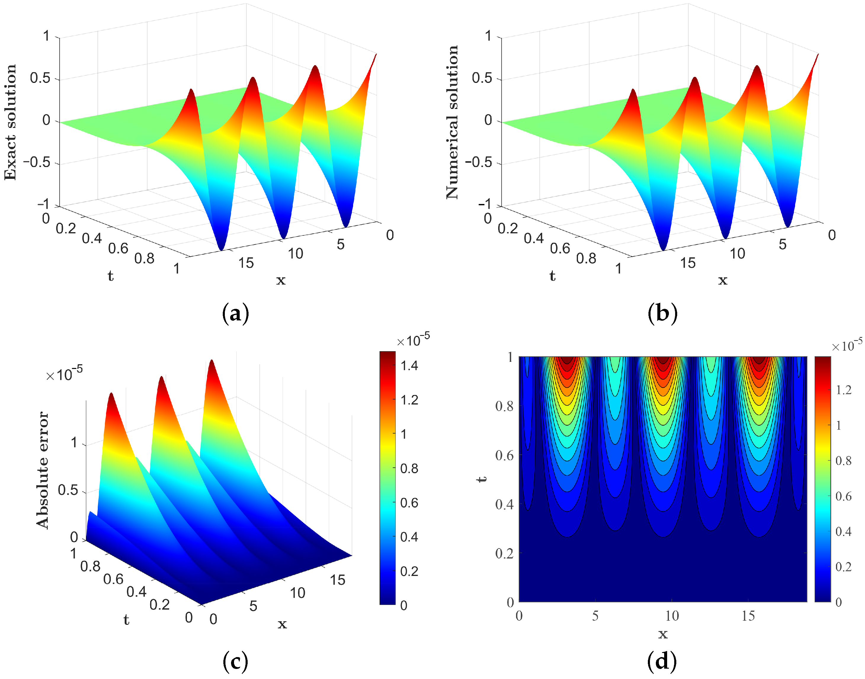
Table 3 presents a detailed comparison of the error and temporal convergence rates for Example 2 with different α values, directly comparing our results with those in [21]. Table 4 presents the error and spatial convergence rates for Example 2 under different M values and α values with N = ( M 2 ) 8 4 α . This analysis is conducted over the domain [ 0 , π ] × [ 0 , 1 ] , highlighting the effectiveness of our method against established results. For plotting and visualization purposes, we employ a different region, [ 0 , 6 π ] × [ 0 , 1 ] , to better highlight the specific features of the solution. This extended domain allows us to observe the periodic nature of the solution more clearly by capturing multiple periods, providing valuable insights into the long-term behavior and periodicity. Additionally, it helps in understanding the boundary effects and their influence on the solution, which is particularly important when boundary conditions significantly impact the overall behavior.
Figure 2 uses the larger domain [ 0 , 6 π ] × [ 0 , 1 ] to illustrate the exact solution, numerical solution, absolute error, and error contour plot for α = 0.99 , M = 200 , and N = 100 . These visualizations further validate the accuracy and convergence of our method under these conditions.
Example 3.
We examine Equation (2) in the domain [ 0 , π ] × [ 0 , 2 ] with d = 1 , p 1 ( x ) = 1 , p 2 ( x ) = 1 , and f ( x , t ) = Γ ( 5 + α ) 24 t 4 cos x + t 4 + α sin x . The exact solution for validation purposes is given by v ( x , t ) = t 4 + α cos x .
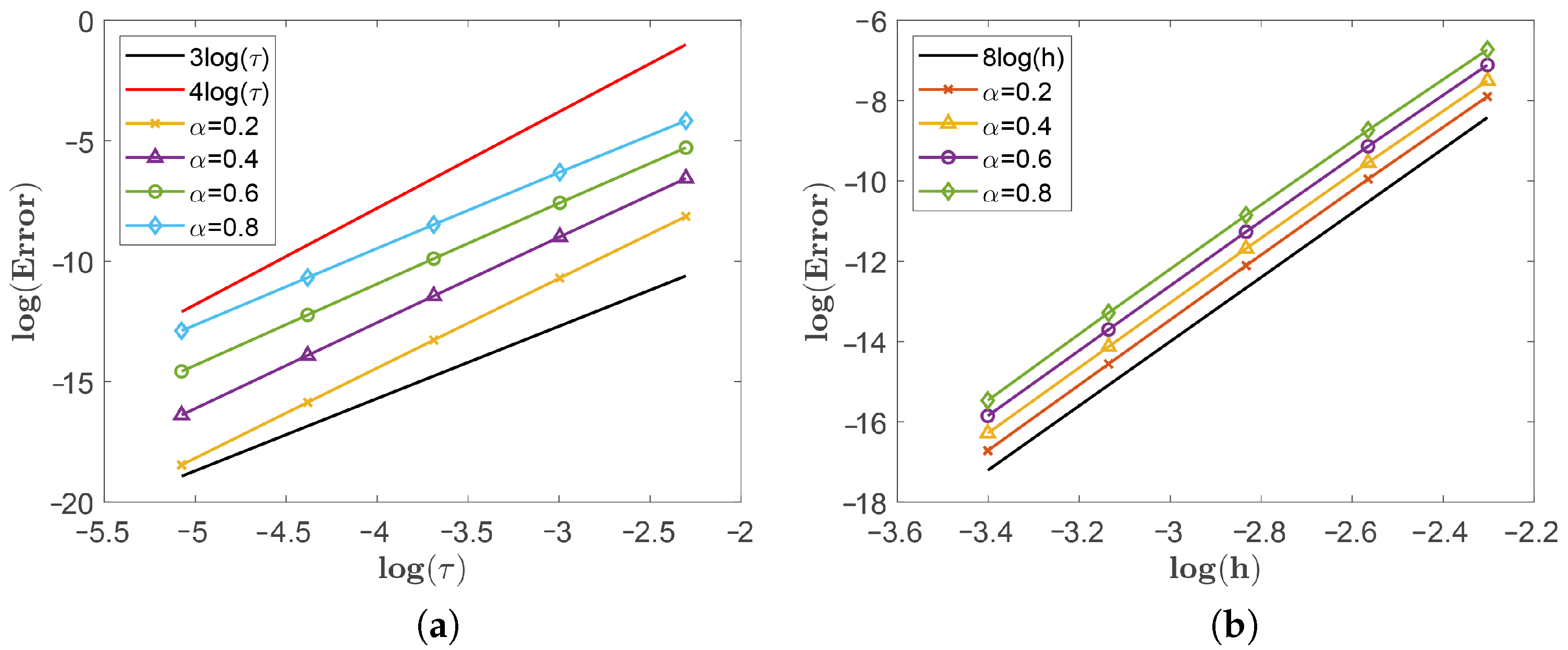
In this final example, we switch to constant coefficients to consolidate our findings from Examples 1 and 2, which deal with variable coefficients. This allows us to reinforce the reliability and robustness of our method across different types of coefficient settings. Table 5 presents the L -error and convergence rates for temporal and spatial discretizations at α = 0.5 . For brevity, we focus on α = 0.5 , though our findings generalize to other α values. This table illustrates the method’s performance under different grid resolutions, demonstrating the expected convergence behavior. Table 6 compares the numerical solutions ( v n ) and exact solutions ( v e ) for different α values and grid points at T = 2 . This comparison provides a direct assessment of the numerical solution’s accuracy across various parameter settings. Figure 3 provides a visual convergence analysis with different α values: (a) l o g ( E r r o r ) vs. l o g ( τ ) for temporal convergence and (b) l o g ( E r r o r ) vs. l o g ( h ) for spatial convergence. These plots further validate the method’s effectiveness and convergence properties for a range of α values, serving as a solid conclusion to our series of examples.

5. Conclusions

In conclusion, we develop a novel numerical scheme for time-fractional CDREs with variable coefficients that combines Lagrange polynomial interpolation for time discretization with a compact finite difference approximation for spatial derivatives. The proposed method exhibits unconditional stability and achieves high-order convergence rates, reaching 4 α -order accuracy in time and eighth-order accuracy in space, as rigorously verified through a Fourier analysis. These results represent a substantial improvement in the numerical solution of fractional partial differential equations. Numerical results validate our theoretical analysis, demonstrating the superior accuracy and efficiency of our method over existing solutions. The present study focuses on 1D problems to establish the foundational accuracy and convergence properties of our method. While this simplifies validation, we acknowledge that extensions to 2D/3D or more complex geometries will require further development, particularly in computational efficiency and boundary condition handling. Additionally, our tests primarily involve linear problems. Application to nonlinear CDREs or real-world scenarios remains a challenge for us. Future work may also explore adaptive mesh strategies and the incorporation of nonlinearity in spatial operators for more realistic modeling.

Author Contributions

Conceptualization, Y.F.; software, Y.F. and L.W.; formal analysis, Y.F. and X.Z.; writing—original draft preparation, Y.F.; writing—review and editing, X.Z. and L.W.; visualization, Y.F. and L.W. All authors have read and agreed to the published version of the manuscript.

Funding

This research was funded by the Scientific Research Foundation for Talents Introduction of Guizhou University of Finance and Economics (No. 2023YJ16); the Institute of Complexity Science, Henan University of Technology (No. CSKFJJ-2025-33); and the Henan Provincial International Science and Technology Cooperation Project (No. 252102520007).

Data Availability Statement

The data analyzed in this study are subject to the following licenses/ restrictions: the first author can receive the restrictions. Requests to access these datasets should be directed to fyl001215@163.com (Y. L. Feng).

Acknowledgments

The authors are very grateful to the referee for carefully reading the article and providing many valuable comments.

Conflicts of Interest

The authors declare no conflicts of interest.

References

  1. Almeida, R.; Bastos, N.R.O.; Monteiro, M.T.T. Modeling some real phenomena by fractional differential equations. Math. Method. Appl. Sci. 2016, 39, 4846–4855. [Google Scholar]
  2. Zhang, Y.; Sun, H.G.; Stowell, H.H.; Zayernouri, M.; Hansen, S.E. A review of applications of fractional calculus in Earth system dynamics. Chaos Soliton. Fract. 2017, 102, 29–46. [Google Scholar]
  3. Failla, G.; Zingales, M. Advanced materials modelling via fractional calculus: Challenges and perspectives. Philos. Trans. R. Soc. A 2020, 378, 2172. [Google Scholar]
  4. Duran, S.; Durur, H.; Yavuz, M.; Yokus, A. Discussion of numerical and analytical techniques for the emerging fractional order Murnaghan model in materials science. Opt. Quant. Electron. 2023, 55, 571. [Google Scholar]
  5. Toledo-Hernandez, R.; Rico-Ramirez, V.; Iglesias-Silva, G.A.; Diwekar, U.M. A fractional calculus approach to the dynamic optimization of biological reactive systems. Part I: Fractional models for biological reactions. Chem. Eng. Sci. 2014, 117, 217–228. [Google Scholar]
  6. Ali, K.K.; Mohamed, M.S.; Maneea, M. Unveiling the dynamics of plasma dilution in medical science through analytical and numerical approaches via fractional integro-differential equations. J. Appl. Math. Comput. 2025, 71, 1219–1245. [Google Scholar]
  7. Das, P.; Mehrmann, V. Numerical solution of singularly perturbed convection-diffusion-reaction problems with two small parameters. BIT Numer. Math. 2016, 56, 51–76. [Google Scholar]
  8. Giere, S.; Iliescu, T.; John, V.; Wells, D. SUPG reduced order models for convection-dominated convection-diffusion-reaction equations. Comput. Method. Appl. M. 2015, 289, 454–474. [Google Scholar]
  9. Chen, G.; Feng, M.F.; Xie, X.P. A robust WG finite element method for convection-diffusion-reaction equations. J. Comput. Appl. Math. 2017, 315, 107–125. [Google Scholar]
  10. Lin, R.C.; Ye, X.; Zhang, S.Y.; Zhu, P. A Weak Galerkin Finite Element Method for Singularly Perturbed Convection-Diffusion-Reaction Problems. SIAM J. Numer. Anal. 2018, 56, 1482–1497. [Google Scholar]
  11. Xu, M.T. A modified finite volume method for convection-diffusion-reaction problems. Int. J. Heat Mass Transf. 2018, 117, 658–668. [Google Scholar]
  12. Zhang, X.D.; Feng, Y.L.; Luo, Z.Y.; Liu, J. A spatial sixth-order numerical scheme for solving fractional partial differential equation. Appl. Math. Lett. 2025, 159, 109265. [Google Scholar]
  13. Feng, Y.L.; Zhang, X.D.; Chen, Y.; Wei, L.L. A compact finite difference scheme for solving fractional Black-Scholes option pricing model. J. Inequal. Appl. 2025, 2025, 36. [Google Scholar]
  14. Li, C.P.; Wang, Z. Numerical methods for the time fractional convection-diffusion-reaction equation. Numer. Func. Anal. Opt. 2021, 42, 1115–1153. [Google Scholar]
  15. Ngondiep, E. A two-level fourth-order approach for time-fractional convection-diffusion-reaction equation with variable coefficients. Commun. Nonlinear Sci. 2022, 111, 106444. [Google Scholar]
  16. Roul, P.; Rohil, V. An efficient numerical scheme and its analysis for the multiterm time-fractional convection-diffusion-reaction equation. Math. Method. Appl. Sci. 2023, 46, 16857–16875. [Google Scholar]
  17. Hosseini, V.R.; Mehrizi, A.A.; Karimi-Maleh, H.; Naddafi, M. A numerical solution of fractional reaction-convection-diffusion for modeling PEM fuel cells based on a meshless approach. Eng. Anal. Bound. Elem. 2023, 155, 707–716. [Google Scholar]
  18. Priyadarshana, S.; Mohapatra, J. An efficient fractional step numerical algorithm for time-delayed singularly perturbed 2D convection-diffusion-reaction problem with two small parameters. Numer. Algorithms 2024, 97, 687–726. [Google Scholar]
  19. Kumar, N.; Toprakseven, S.; Jiwari, R. A numerical method for singularly perturbed convection-diffusion-reaction equations on polygonal meshes. Comput. Appl. Math. 2024, 43, 44. [Google Scholar]
  20. Liu, M.M.; Zheng, X.C.; Li, K.X.; Qiu, W.L. High-order compact difference method for convection-reaction-subdiffusion equation with variable exponent and coefficients. Numer. Algorithms 2025. [Google Scholar] [CrossRef]
  21. Ren, L.; Wang, Y.M. A fourth-order extrapolated compact difference method for time-fractional convection-reaction-diffusion equations with spatially variable coefficients. Appl. Math. Comput. 2017, 312, 1–22. [Google Scholar]
  22. Abdi, N.; Aminikhah, H.; Refahi Sheikhani, A.H. High-order compact finite difference schemes for the time-fractional Black-Scholes model governing European options. Chaos Soliton. Fract. 2022, 162, 112423. [Google Scholar]
  23. Kumari, S.; Singh, A.K.; Mehandiratta, V.; Mehra, M. High-order approximation to Caputo derivative on graded mesh and time-fractional diffusion equation for nonsmooth solutions. J. Comput. Nonlin. Dyn. 2024, 19, 10. [Google Scholar]
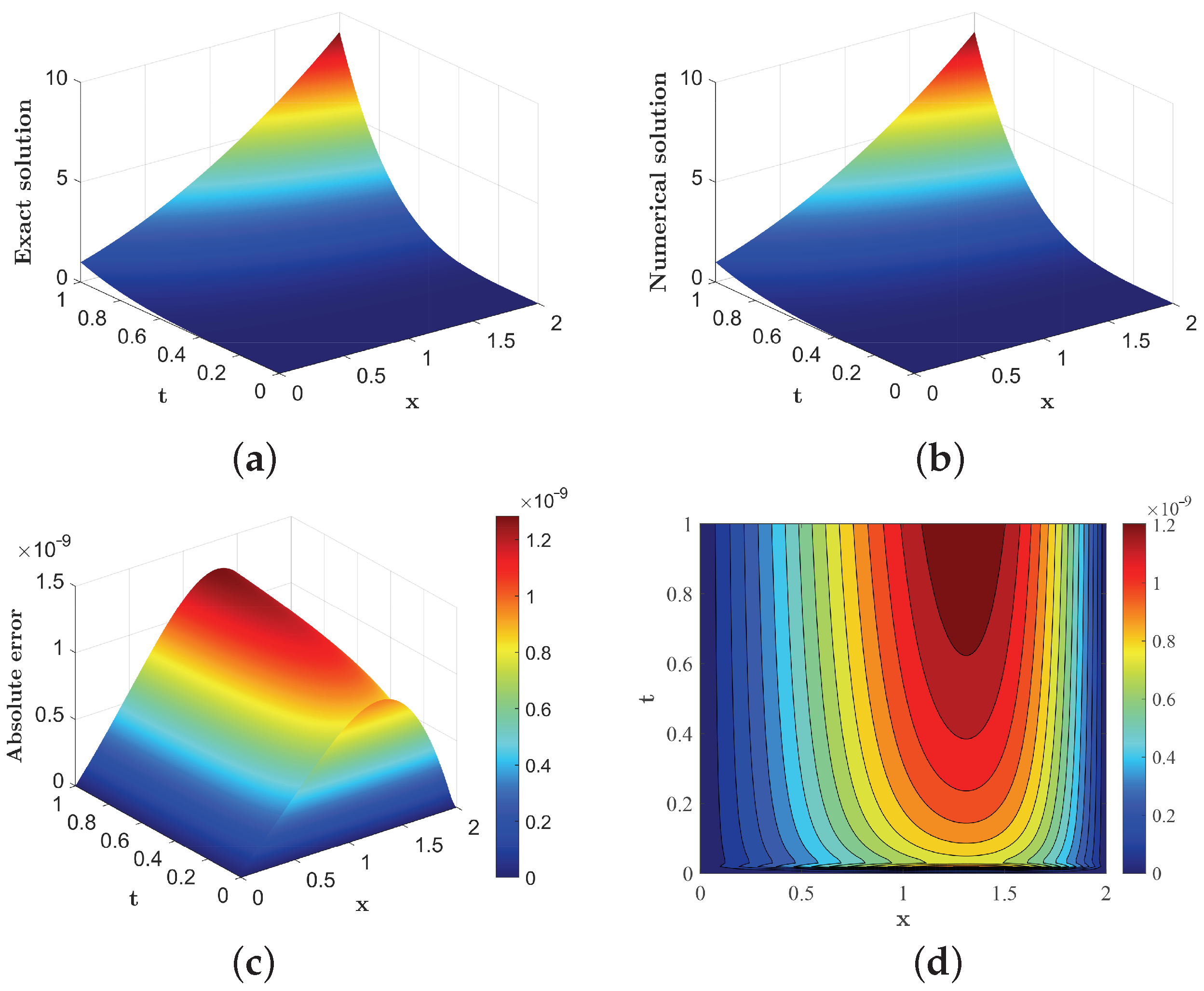
Figure 1. Visualization of Example 1 with α = 0.01 , M = 100 , and N = 100 : (a) exact solution; (b) numerical solution; (c) absolute error; (d) contour plot of error.
Fractalfract 09 00451 g001
Figure 2. Visualization of Example 2 with α = 0.99 , M = 200 , and N = 100 : (a) exact solution; (b) numerical solution; (c) absolute error; (d) contour plot of error.
Fractalfract 09 00451 g002
Figure 3. Convergence analysis with different α values: (a) log( E r r o r ) vs. log( τ ) for temporal convergence; (b) log( E r r o r ) vs. log(h) for spatial convergence.
Fractalfract 09 00451 g003
Table 1. Comparison of error and temporal convergence rates for Example 1 at M = 100 .
N α = 0.25 α = 0.5 α = 0.75
L -Error L -Rate L -Error L -Rate L -Error L -Rate
[21]402.5734 × 10 5 8.3385 × 10 5 1.9864 × 10 4
803.2434 × 10 6 2.98811.0540 × 10 5 2.98392.5199 × 10 5 2.9787
1604.0709 × 10 7 2.99411.3249 × 10 6 2.99203.1730 × 10 6 2.9894
3205.0989 × 10 8 2.99711.6607 × 10 7 2.99603.9807 × 10 7 2.9947
Our403.8755 × 10 6 3.0304 × 10 5 1.7518 × 10 4
802.9991 × 10 7 3.69182.7402 × 10 6 3.46721.8793 × 10 5 3.2206
1602.2996 × 10 8 3.70512.4561 × 10 7 3.47981.9964 × 10 6 3.2347
3201.7106 × 10 9 3.74882.1851 × 10 8 3.49062.1095 × 10 7 3.2424
Table 2. Comparison of error and spatial convergence rates for Example 1.
M α = 0.25 α = 0.5 α = 0.75
L -Error L -Rate L -Error L -Rate L -Error L -Rate
[21]87.1868 × 10 8 5.6976 × 10 8 4.4166 × 10 8
164.5156 × 10 9 3.99243.5806 × 10 9 3.99212.7763 × 10 9 3.9917
322.8239 × 10 10 3.99922.2351 × 10 10 4.00181.7308 × 10 10 4.0036
641.7339 × 10 11 4.02551.3457 × 10 11 4.05391.0351 × 10 11 4.0635
Our81.0969 × 10 2 3.4659 × 10 2 6.6072 × 10 2
165.9367 × 10 5 7.52951.7548 × 10 4 7.62584.3821 × 10 4 7.2363
322.5068 × 10 7 7.88777.5292 × 10 7 7.86461.7378 × 10 6 7.9782
641.0027 × 10 9 7.96583.0181 × 10 9 7.96276.2153 × 10 9 8.1273
Table 3. Comparison of error and temporal convergence rates for Example 2 with different α values.
M × N α = 0.25 α = 0.5 α = 0.75
L -Error L -Rate L -Error L -Rate L -Error L -Rate
[21]1000 × 402.7763 × 10 6 9.0510 × 10 6 2.1821 × 10 5
1000 × 803.4991 × 10 7 2.98811.1439 × 10 6 2.98412.7671 × 10 6 2.9793
1000 × 1604.3916 × 10 8 2.99411.4378 × 10 7 2.99213.4835 × 10 7 2.9897
1000 × 3205.4995 × 10 9 2.99741.8021 × 10 8 2.99614.3698 × 10 8 2.9949
Our200 × 404.1605 × 10 7 3.2513 × 10 6 1.8881 × 10 5
200 × 803.2193 × 10 8 3.69202.9393 × 10 7 3.46752.0243 × 10 6 3.2215
200 × 1602.4677 × 10 9 3.70552.6341 × 10 8 3.48012.1497 × 10 7 3.2352
200 × 3201.8287 × 10 10 3.75432.3426 × 10 9 3.49112.2711 × 10 8 3.2427
Table 4. Error and spatial convergence rates for Example 2 with different α values and N = ( M 2 ) 8 4 α .
M α = 0.25 α = 0.5 α = 0.75
L -Error L -Rate L -Error L -Rate L -Error L -Rate
162.2560 × 10 4 7.8067 × 10 4 1.5142 × 10 3
249.3857 × 10 6 7.84182.9720 × 10 5 8.06076.6303 × 10 5 7.7157
329.3441 × 10 7 8.01932.9686 × 10 6 8.00796.7649 × 10 6 7.9340
401.5472 × 10 7 8.05894.8711 × 10 7 8.09951.1578 × 10 6 7.9106
Table 5. L -error and temporal/spatial convergence rates for Example 3 at α = 0.5 .
Temporal ConvergenceSpatial Convergence
M × N L -Error L -Rate M × N L -Error L -Rate
100 × 10 7.4329 × 10 3 10 × 1000 3.4979 × 10 4
100 × 20 7.0324 × 10 4 3.4018 15 × 1000 1.4734 × 10 5 7.8112
100 × 40 6.4632 × 10 5 3.4437 20 × 1000 1.4621 × 10 6 8.0308
100 × 80 5.8474 × 10 6 3.4664 25 × 1000 2.4045 × 10 7 8.0893
Table 6. Comparison of numerical solutions ( v n ) and exact solutions ( v e ) for Example 3.
x α = 0.01 α = 0.5 α = 0.99
v n v e v n v e v n v e
π 8 14.8848899714.8848899720.9050083120.9050074429.3599871029.35993057
2 π 8 11.3924015711.3924015616.0000004116.0000000022.4711565422.47111801
3 π 8 6.165523306.165523308.659136898.6591376012.1612633612.16128143
4 π 8 0.000000000.00000000−0.000001880.00000000−0.000080260.00000000
5 π 8 −6.16552330−6.16552330−8.65914020−8.65913760−12.16140299−12.16128143
6 π 8 −11.39240157−11.39240156−16.00000257−16.00000000−22.47124269−22.47111801
7 π 8 −14.88488997−14.88488997−20.90500912−20.90500744−29.36001345−29.35993057
Disclaimer/Publisher’s Note: The statements, opinions and data contained in all publications are solely those of the individual author(s) and contributor(s) and not of MDPI and/or the editor(s). MDPI and/or the editor(s) disclaim responsibility for any injury to people or property resulting from any ideas, methods, instructions or products referred to in the content.