Abstract
In this work, we investigate the extended numerical discretization technique for the solution of fractional Bernoulli equations and SIRD epidemic models under the Caputo fractional, which is accurate and versatile. We have demonstrated the method’s strength in examining complex systems; it is found that the method produces solutions that are identical to the exact solution and approximate series solutions. The ENDT is its ability to proficiently handle complex systems governed by fractional differential equations while preserving memory and hereditary characteristics. Its simplicity, accuracy, and flexibility render it an effective instrument for replicating real-world phenomena in physics and biology. The ENDT method offers accuracy, stability, and efficiency compared to traditional methods. It effectively handles challenges in complex systems, supports any fractional order, is simple to implement, improves computing efficiency with sophisticated methodologies, and applies it to epidemic predictions and biological simulations.
1. Introduction
Fractional calculus, involving non-integer orders of derivatives and integrals, has developed rapidly in recent decades in science and engineering [,]. They extend the classical calculus so that one can model problems that the standard approach cannot [,]. Fractional derivatives have turned out to be crucial because they can help solve some real-world problems. It has opened up new areas of theoretical opportunities and practical applications in physics, control theory, signal processing, materials science, and biological modeling [,,,,,,].
In contrast to traditional calculus, fractional calculus can describe systems with memory and hereditary features, making it popular in recent decades. Currently, it is widely applied in physics, engineering, biology, finance, etc. Fractional calculus improves long-term memory modeling and offers improvements in control theory. Fractional-time derivatives explain the relationship between stresses and strains in viscoelastic materials [,,]. In biomedical sciences, fractional models are more flexible and accurate for disease propagation than integer-order models. The applications of FC are expanding and crucial for scientific and technical research [,,], emerging as a versatile tool [,].
Epidemiological models are the basis for infectious disease dynamics and allow researchers and policymakers to predict how a disease spreads, perform impact assessments, and evaluate intervention strategies. These integrate mathematical frameworks into real data to simulate the behavior of diseases in alternative scenarios [,]. Given the complexity of infectious diseases, which depend on parameters such as transmission rates, population mobility, and environmental conditions, formulation and simulation have become an integrated part of effective public health planning [,]. With the use of advanced numerical techniques and computational simulations, studies on the impact of all control measures, vaccination campaigns, quarantine protocols, and treatment strategies under various conditions could be made. The ability to model these scenarios provides great insight into how to reduce the impact of outbreaks and maintain health resources effectively. The role of simulations in epidemiology has grown dramatically, with rapid improvements in technology and mathematical modeling techniques that provide strong tools to solve global health problems [,].
Research on the derivation of efficient and accurate numerical algorithms for solving problems composed of ODEs has recently shown increasingly rapid development [,,,]. Several discretization schemes were introduced, according to [,,,], for special types of time-fractional PDEs. In most cases, these discretization techniques, for both integer-order and time-fractional ODEs, form a large linear or nonlinear system where unknowns approximate solution values at interior mesh points.
This article shows an innovative way to solve a fractional-order Bernoulli equation and a fractional epidemic model that includes susceptible, infected, recovered, and dead (SIRD) cases. It carries this out by using a scheme of fractional-order time derivatives. We demonstrate the efficiency and accuracy of the developed method by comparing approximate solutions with exact solutions, resulting in a perfect match. The proposed approach represents a new avenue to extend fractional-order methods to a wide class of systems with high-accuracy solutions. In the near future, this may be a very promising approach to developing and realizing complex fractional models in different fields, such as physics and engineering.
2. Basic Principles
This section defines the Riemann–Liouville and Caputo operators, which form the foundation for fractional differential equations used.
Definition 1.
The Riemann–Liouville (R-L) fractional integral operator of order is defined as follows []:
Definition 2.
Applying the Riemann–Liouville (R-L) operators, and are given by []
Definition 3.
For α (), Caputo operators are used [].
3. The Extended Numerical Discretization Technique (ENDT)
These methods assume the initial value problem for .
is equivalent to the Volterra-type integral equation []:
3.1. Numerical Approximation Framework
To solve different kinds of ordinary differential equations (ODEs), many numerical methods with discretization schemes have been created [,,]. Researchers have been working on making numerical schemes that are both efficient and reliable for solving ODEs for a long time because they are useful in both engineering and science. Typically, most discretization schemes that are used to numerically solve ODEs end up in algebraic systems where the unknowns are approximations at discrete time steps. This article describes an ODE’s discretization scheme by reducing the computational complexity through minimizing the solution of large-scale equations of systems and, therefore, an effective applied strategy to solve initial value problems.
where G depends on , , and is the Caputo operator () for variable t, with , and boundary conditions (BCs) .
We use finite differences to reduce (6) to ODEs, then solve them using the fractional Adams method, analyze the stability (see []), and finally, validate via simulations. Assuming , we discretize with grid , , and approximate and using finite differences.
with (), yielding ODEs:
To solve Equation (8), we extend the fractional Adams method to handle the equations. Specifically, for each , we can compute based on the equivalence of the initial value problem to the integral equation, expressed as follows for :
The corrector step is given by
where
and
The predictor step, which is crucial in evaluating , involves applying the fractional Adams–Bashforth method to Equation (11), yielding the predictor value:
We outline the steps to approximate . The scheme is simple for all values of , with computed using previously known values without solving equations. This method can also be applied to other integer- and fractional-order IBVPs using divided differences for derivatives of u.
3.2. Stability Analysis
If the aim is for an initial value problem (IVP) solver to be numerically stable, then it should be ensured that small changes in the initial conditions do not cause big changes in the solutions obtained [,]. In the following analysis, we consider the scheme’s stability.
Theorem 1.
Assume satisfies Lipschitz conditions with respect to its variables as
Proof.
From (15),
For each , set , and then we get
and so,
where
Using the discrete Grönwall’s inequality, we obtain
For weights and (), the relations are
Using (25) and (26), Equation (27) simplifies to
Finally, the constant K in Equation (20) is set as
Thus, we obtain the desired result. Since G satisfies the Lipschitz condition, there exists a positive constant k such that, following a similar approach, we can prove . □
4. Numerical Results from Simulations
The work at hand proposes a new schema to solve two completely different problems: the Bernoulli equation and epidemic disease models. Given its widespread application in fluid dynamics, thermodynamics, and various other scientific fields, we begin with the Bernoulli equation. Here, we propose an innovative approach to the search for solutions by taking advantage of advanced techniques and algorithms and offering new insight into this classical problem. We next consider epidemic disease models, which have been gaining increasing importance in formulating the dynamics of infectious diseases. With our new schema applied to such models, we would like to make predictions of disease spread more accurately and efficiently while determining the best strategies for its control. Mathematical modeling will be combined with computational methods in order to obtain more reliable predictions in the context of real-world epidemics. We use our schema to solve the Bernoulli equation and models of epidemic diseases to show how useful and powerful this approach is for solving a wide range of difficult problems.
Problem 1.
We start with the Fractional Bernoulli equation []:
where and . The exact solution of the Bernoulli equation, when is
under the initial condition , where is defined by Equation (4) with the parameter α. When , the Bernoulli Equation (29) has an exact solution corresponding to the proposed numerical approach.
Table 1 shows the numerical solutions of the Bernoulli equation for various values of N and T at . The results show the behavior of the proposed numerical method for the approximating solution to the exact solution . It can be seen that as the number of grid points N is increased, the numerical solution starts converging toward the exact solution for all the tested values of . This demonstrates the accuracy and stability of the method at large resolutions. For example, the solution with is very accurate and has a negligible difference from the exact solution at . At , for all N continuously, the numerical method agrees with the exact solution, reflecting its reliability for large time intervals.

Table 1.
Numerical solutions of the Bernoulli equation at .
The numbers in Table 2 are the answers to the Bernoulli equation for the fractional order at different times , when the grid sizes are N. The results show that the method converges as N increases, and they also show that it works well for solving problems with fractional orders close to 1. The following examples demonstrate that the accuracy of numerical solutions tends to increase as N increases. For , the solution for is closer to the exact solution than coarser grids like . A similar trend is seen for and , where the solution successively approaches for increasing N.
Table 2.
Numerical solutions of the Bernoulli equation at .
The numbers in Table 3 below show the answers to the Bernoulli equation when , with the corresponding values of T and N. For N = 50 to 600, the solutions converge, and the successive values almost overlap, indicating that the precision is stable and effective. The solutions tend to a stable number for each T, and the divergence becomes small for higher N, particularly for and . Additionally, the solutions improve as T decreases, with values slightly higher at compared to those at . This shows that T changes how the equations behave. In general, the findings show that the numerical technique is reliable and stable, with the equation stabilizing for higher values of N and the solutions becoming more accurate as N grows.
Table 3.
Numerical solutions of the Bernoulli equation at .
However, it is also clear that the fractional order introduces a small but consistent deviation from the exact solution observed at the integer order . Thus, even for slight variations in the order, that difference reflects the expected sensitivity for fractional-order systems. The method retains robustness in capturing those subtle differences while keeping accuracy high.
These two graphs in Figure 1 compare exact (solid line) and approximate (dashed line) solutions of the system in Equation (27) for values of 1 (left) and 0.99 (right), with time t. Both cases show nearly identical behavior. The remarkable overlap between exact and approximate solutions in both scenarios validates the novel method’s accuracy.
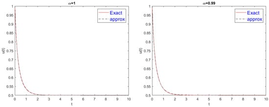
Figure 1.
Comparison of exact and approximate solutions for Equation (29).
Problem 2.
We discuss the model of epidemic disease as follows []:
We define the parameters and ψ, each representing a specific rate related to disease dynamics: β indicates the infection rate of susceptible individuals, valued at 0.0007; δ represents the recovery rate of infected individuals, set at 0.09; and ψ denotes the mortality rate of infected individuals, established at 0.08.
When setting the initial conditions, it is presumed that the total population, represented by N, does not change over time. This assumption implies that the population at the initial time is the combined sum of individuals in each compartment: susceptible, infected, recovered, and deceased. Mathematically, this relationship is described by the equation , where , , , and represent the initial numbers in each respective group. We assume initial conditions , , , and (see []). The choice of the fractional order α is based on the fact that it is able to capture the memory effect and anomalous dynamics that occur in the propagation of infectious diseases. For this study, α is selected in the range to represent subdiffusive behavior, with smaller values of α producing stronger memory effects. The specific value of α is chosen to yield the best fit for the epidemic data observed or simulated, such that the model describes real dynamics.
Table 4 gives the susceptible population in time t for different values of . At first (), the population is uniformly distributed as 350 and decreases with increasing t according to the value of . When , the decrease occurs quickly, whereas the smaller the , the slower the decrease; this reflects a moderating effect from fractional dynamics. This reveals the flexibility of the fractional-order model to capture the behaviors of epidemics, particularly in systems that have memory or hereditary effects.
Table 4.
Susceptible population for different fractional orders .
Table 5 shows the infected population as a function of time, t, for different values of . For , all the values have an infected population of 400, providing a consistent initial condition. As t increases, the infected population grows consistently for all , with higher values, for example, exhibits a faster growth rate compared to lower values. This trend reflects the impact of fractional-order dynamics, where smaller values of lead to a dampened development of infections, likely reflecting memory effects or delays in the spread. These results confirm the flexibility of fractional-order models to represent different infection dynamics.
Table 5.
Infected population for different fractional orders .
Table 6 presents variations in the recovered population with respect to time, t, for different values of . When , the recovered population is always 400 for all values. As time t increases, the recovered population in all cases decreases; however, the smaller the value, the slower the decline in the recovered population compared to higher values. This would confirm that the underlying dynamics are of fractional order, and a smaller value of indicates a more delayed or moderated recovery process. These results highlight the flexibility of the fractional-order models in modeling the recovery patterns driven by memory or hereditary effects.
Table 6.
Recovered population for different fractional orders .
Table 7 presents the dead population over time (t) for various values of . For , all the values have a population of 350, which acts as a uniform starting point. For larger t, the dead population decreases with increasing rates across different values of . A higher value of , for example, , gives a faster decline in the dead population, whereas a smaller value of exhibits a slower decay, which may reveal the contribution of fractional-order dynamics in controlling mortality rates. These findings highlight the utility of fractional-order models in capturing nuanced death dynamics driven by memory effects or varied characteristics of the system.
Table 7.
Dead population for different fractional orders .
Figure 2 shows the epidemic model simulations, demonstrating population dynamics under varying fractional-order derivatives () over a 100-day period. The system shows well-separated behavioral patterns: for higher values, such as 1.0 and 0.95, the populations have rapid initial decline with a stabilization around day 40 and are characterized by lower final population values and more complete resolution of the disease. Lower values of , such as 0.75 and 0.55, show a more gradual decline in curves, with higher sustained populations and incomplete resolution at day 100. All four cases start with population peaks around 400–450 individuals, where susceptible (S, blue) and infected (I, red) populations immediately show steep declines, while recovery (R, green) and death (D, cyan) are proportional to . The model serves to illustrate the impact of different intervention intensities of the value on the course of disease progression and resolution. Higher values correspond to more aggressive intervention strategies that yield faster containment of the disease but perhaps higher initial mortality rates, while lower values suggest more moderate interventions, leading to a prolonged presence of the disease but perhaps more manageable healthcare demands over time.
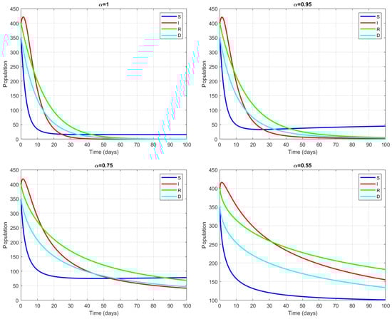
Figure 2.
Four views of the system for different values of .
5. Numerical Method Accuracy
In this part, we find the numerical accuracy of the model from above by calculating the error in every compartment S, I, R, and D with the assistance of the following formula:
where is the norm, or the maximum absolute error at any time step. This is found by comparing values at two time step sizes, and , to evaluate the impact of halving the time step on accuracy. The respective errors for different step sizes () and fractional orders () are provided in Table 8 and Table 9. The aim of this research is to verify the convergence of the numerical scheme and find out how modifications in the time step and fractional order affect the precision of the solution. Through a comparison of errors at different , we can examine the behavior of convergence for the algorithm, while studying the influence of helps one consider how the dynamics of the model are affected by fractional derivatives. This error analysis is crucial in order to make the optimal trade-off between efficiency of computation and accuracy, especially in real applications, such as epidemiological models, where the choice of the numerical parameters highly influences the reliability of the results.
Table 8.
Errors of S, I, R, D at and .
Table 9.
Errors of S, I, R, D at and .
In Table 8, the errors for at are presented. From these results, one can observe the tendency of convergence as the step size decreases. The error values for and D approximately halve each time is halved, which aligns well with the expectations based on the numerical accuracy for this type of fractional model. Among the compartments, the error is highest for S, while and D exhibit comparable magnitudes.
In Table 9, at for , the errors are larger compared to the case for , indicating greater complexity in the dynamics at fractional orders. The halving of yields a significant reduction in the error across all compartments, confirming the model’s reliability for fractional-order systems. The error for S remains dominant, while and D follow a similar trend.
6. Discussion
Fractional integral equations were successfully solved via the fractional calculus method by using various analytical and numerical methods such as Grűnwald–Letnikov, finite element, and spectral ones. However, such techniques typically have problems with stability, convergence, and computing complexity.
The numerical discretization of the Grünwald–Letnikov difference (ENDT), a newly proposed method in this study, was found to be more accurate and efficient, particularly in allowing us to overcome the above concerns in chaotic and hyperchaotic systems. In contrast with traditional methods, ENDT is capable of ensuring the best rates of accuracy and stability when solving both Caputo IVP and boundary value problems (BVPs) through Caputo-type fractional derivatives. One of the applications illustrating the robustness and predictability of ENDT in all the series of models is through numerical simulations.
The method is meant to be global, with tools to be used for any fractional order, and this, of course, is given a limited domain. The positive numerical results show that ENDT is technically proficient and can be a useful tool for the precise solution of generalized fractional differential equations in several engineering and scientific applications.
The ENDT approach provides great precision, stability, and efficiency. By guaranteeing higher convergence, simplicity of implementation, and more general applicability in physics, biology, and engineering, it beats conventional approaches.
This research introduces an extended numerical discretization technique (ENDT) that solves fractional Bernoulli equations and SIRD epidemic models subject to Caputo fractional derivatives with the highest accuracy and stability. ENDT accurately matches series solutions and handles memory and heredity difficulties more efficiently than typical approaches. The approach may be used for stochastic and multidimensional systems in physics, biology, and engineering. The method’s speed, variety, and reliability make it a powerful tool for solving difficult fractional differential equation problems, especially in daily settings like epidemic prediction and biological system modeling.
7. Conclusions
The extended numerical discretization technique for the solution of fractional Bernoulli equations and SIRD epidemic models under the Caputo fractional initial value problem, as discussed in the present study, is immensely accurate and versatile. The method presented has been shown to be a strong way to look at complicated systems that are controlled by FDEs. It provides solutions that are consistent, with exact results and very accurate approximate series solutions. Its memory capability and hereditary properties make it a useful tool for analyzing dynamics in physics, biology, and engineering. Furthermore, its adaptability suggests possible extensions to more intricate systems, including stochastic and multidimensional models. More research will be carried out on how to use this method for larger problems, how to combine it with more advanced computer methods, and how to use it in the real world for applications like predicting epidemics and simulating biological systems. This development opens new pathways for finding new approaches to solving complicated scientific problems. Future work will expand the suggested method to more complicated and stochastic systems, improve computing efficiency with sophisticated methodologies, and apply it to epidemic predictions and biological simulations.
Author Contributions
Methodology, R.A.; Validation, S.S.A.; Formal analysis, R.A. and S.S.A.; Supervision, R.A.; Writing—original draft, R.A.; Writing—review and editing, S.S.A. All authors have read and agreed to the published version of the manuscript.
Funding
This research received no external funding.
Data Availability Statement
The original contributions presented in this study are included in the article.
Conflicts of Interest
The authors declare no conflicts of interest.
References
- Sun, H.; Zhang, Y.; Baleanu, D.; Chen, W.; Chen, Y. A new collection of real-world applications of fractional calculus in science and engineering. Commun. Nonlinear Sci. Numer. Simul. 2018, 64, 213–231. [Google Scholar] [CrossRef]
- Chen, W.; Sun, H.; Li, X. Fractional Derivative Modeling in Mechanics and Engineering; Springer: Berlin/Heidelberg, Germany, 2022. [Google Scholar]
- Agarwal, R.; Purohit, S.D.; Kritika. Introduction to Fractional Calculus and Modelling. In Modeling Calcium Signaling: A Fractional Perspective; Springer: Berlin/Heidelberg, Germany, 2024; pp. 1–28. [Google Scholar]
- Mohammad, M.; Saadaoui, M. A new fractional derivative extending classical concepts: Theory and applications. Partial. Differ. Equations Appl. Math. 2024, 11, 100889. [Google Scholar] [CrossRef]
- Saadeh, R.; Khalil, R.; Baqaien, R.; Qazza, A. Solving system of ODEs and analyzing chemical reactions. Eng. Lett. 2025, 33. [Google Scholar]
- Karatetskaia, E.; Kazakov, A.; Safonov, K.; Turaev, D. Robust chaos in a totally symmetric network of four phase oscillators. arXiv 2024, arXiv:2408.06435. [Google Scholar] [CrossRef]
- Berir, M. The impact of white noise on chaotic behavior in a financial fractional system with constant and variable order: A comparative study. Eur. J. Pure Appl. Math. 2024, 17, 3915–3931. [Google Scholar] [CrossRef]
- Alzahrani, S.M.; Guma, F.E. Improving seasonal influenza forecasting using time series machine learning techniques. J. Inf. Syst. Eng. Manag. 2024, 9, 30195. [Google Scholar] [CrossRef]
- Abdoon, M.A.; Alzahrani, A.B.M. Comparative analysis of influenza modeling using novel fractional operators with real data. Symmetry 2024, 16, 1126. [Google Scholar] [CrossRef]
- Alsubaie, N.E.; EL Guma, F.; Boulehmi, K.; Al-kuleab, N.; Abdoon, M.A. Improving influenza epidemiological models under Caputo fractional-order calculus. Symmetry 2024, 16, 929. [Google Scholar] [CrossRef]
- Abdulkream Alharbi, S.; Abdoon, M.A.; Saadeh, R.; Alsemiry, R.D.; Allogmany, R.; Berir, M.; EL Guma, F. Modeling and analysis of visceral leishmaniasis dynamics using fractional-order operators: A comparative study. Math. Methods Appl. Sci. 2024, 47, 9918–9937. [Google Scholar] [CrossRef]
- Olayiwola, M.O.; Alaje, A.I.; Yunus, A.O. Modelling the impact of education and memory on the management of diabetes mellitus using Atangana-Baleanu-Caputo fractional order model. Nonlinear Dyn. 2025, 113, 9165–9185. [Google Scholar] [CrossRef]
- Ahmed, G. Analysis and applications of the chaotic hyperbolic memristor model with fractional order derivative. Eur. J. Pure Appl. Math. 2024, 17, 835–851. [Google Scholar] [CrossRef]
- Hristov, J. Fractional modeling approaches to transport phenomena: Causality, fading memory, and Volterra equations. In Computation and Modeling for Fractional Order Systems; Elsevier: Amsterdam, The Netherlands, 2024; pp. 41–71. [Google Scholar]
- Elbadri, M. An approximate solution of a time fractional Burgers’ equation involving the Caputo-Katugampola fractional derivative. Partial. Differ. Equations Appl. Math. 2023, 8, 100560. [Google Scholar] [CrossRef]
- Ige, O.E.; Oderinu, R.A.; Elzaki, T.M. Adomian polynomial and Elzaki transform method of solving fifth order Korteweg-de Vries equation. Casp. J. Math. Sci. 2019, 8, 103–119. [Google Scholar]
- Magzoub, M.; Elzaki, T.M.; Chamekh, M. An innovative method for solving linear and nonlinear fractional telegraph equations. Adv. Differ. Equations Control. Process. 2024, 31, 651–671. [Google Scholar] [CrossRef]
- Tarasov, V.E. On history of mathematical economics: Application of fractional calculus. Mathematics 2019, 7, 509. [Google Scholar] [CrossRef]
- Qawaqneh, H. Fractional analytic solutions and fixed point results with some applications. Adv. Fixed Point Theory 2024, 14, 1. [Google Scholar]
- Ebulue, C.C.; Ekkeh, O.V.; Ebulue, O.R.; Ekesiobi, C.S. Environmental data in epidemic forecasting: Insights from predictive analytics. Comput. Sci. Res. J. 2024, 5, 1113–1125. [Google Scholar]
- Zhao, A.P.; Li, S.; Cao, Z.; Hu, P.J.-H.; Wang, J.; Xiang, Y.; Xie, D.; Lu, X. AI for science: Predicting infectious diseases. J. Saf. Sci. Resil. 2024, 5, 130–146. [Google Scholar] [CrossRef]
- Bedi, J.S.; Vijay, D.; Dhaka, P.; Gill, J.P.S.; Barbuddhe, S.B. Emergency preparedness for public health threats, surveillance, modelling and forecasting. Indian J. Med. Res. 2021, 153, 287–298. [Google Scholar] [CrossRef]
- Jiang, X.; Ye, D.; Lan, W.; Luo, Y. Epidemic, Urban Planning and Health Impact Assessment: A Linking and Analyzing Framework. Buildings 2024, 14, 2141. [Google Scholar] [CrossRef]
- Alahmadi, A.; Belet, S.; Black, A.; Cromer, D.; Flegg, J.A.; House, T.; Jayasundara, P.; Keith, J.M.; McCaw, J.M.; Moss, R.; et al. Influencing public health policy with data-informed mathematical models of infectious diseases: Recent developments and new challenges. Epidemics 2020, 32, 100393. [Google Scholar] [CrossRef] [PubMed]
- Hrzic, R.; Cade, M.V.; Wong, B.L.H.; McCreesh, N.; Simon, J.; Czabanowska, K. A competency framework on simulation modelling-supported decision-making for Master of Public Health graduates. J. Public Health 2024, 46, 127–135. [Google Scholar] [CrossRef]
- Donatelli, M.; Mazza, M.; Serra-Capizzano, S. Spectral analysis and multigrid methods for finite volume approximations of space-fractional diffusion equations. SIAM J. Sci. Comput. 2018, 40, A4007–A4039. [Google Scholar]
- Li, C.; Hon, S. Multilevel Tau preconditioners for symmetrized multilevel Toeplitz systems with applications to solving space fractional diffusion equations. SIAM J. Matrix Anal. Appl. 2025, 46, 487–508. [Google Scholar] [CrossRef]
- She, Z.-H.; Qiu, Y.-F.; Chen, X.; Lin, F.-R. An IRK-QCD scheme for the space fractional diffusion equation and block-lower-triangle preconditioners for the corresponding linear systems. Numer. Linear Algebra Appl. 2025, 32, e2605. [Google Scholar] [CrossRef]
- Elbadri, M.; AlMutairi, D.M.; Almutairi, D.K.; Hassan, A.A.; Hdidi, W.; Abdoon, M.A. Efficient numerical techniques for investigating chaotic behavior in the fractional-order inverted Rössler system. Symmetry 2025, 17, 451. [Google Scholar] [CrossRef]
- Odibat, Z. On the numerical discretization of the fractional advection-diffusion equation with generalized Caputo-type derivatives on non-uniform meshes. Commun. Appl. Math. Comput. 2024, 1–19. [Google Scholar] [CrossRef]
- Ghanbari, B.; Atangana, A. An efficient numerical approach for fractional diffusion partial differential equations. Alex. Eng. J. 2020, 59, 2171–2180. [Google Scholar] [CrossRef]
- Odibat, Z. Numerical solutions of linear time-fractional advection-diffusion equations with modified Mittag-Leffler operator in a bounded domain. Phys. Scr. 2023, 99, 015205. [Google Scholar] [CrossRef]
- Allogmany, R.; Ismail, F. Implicit three-point block numerical algorithm for solving third order initial value problem directly with applications. Mathematics 2020, 8, 1771. [Google Scholar] [CrossRef]
- Podlubny, I. Fractional Differential Equations: An Introduction to Fractional Derivatives, Fractional Differential Equations, to Methods of Their Solution and Some of Their Applications; Elsevier: Amsterdam, The Netherlands, 1998. [Google Scholar]
- Caputo, M.; Fabrizio, M. A new definition of fractional derivative without singular kernel. Prog. Fract. Differ. Appl. 2015, 1, 73–85. [Google Scholar]
- Diethelm, K.; Ford, N.J.; Freed, A.D. A predictor-corrector approach for the numerical solution of fractional differential equations. Nonlinear Dyn. 2002, 29, 3–22. [Google Scholar] [CrossRef]
- Zabidi, N.A.; Majid, Z.A.; Kilicman, A.; Ibrahim, Z.B. Numerical solution of fractional differential equations with Caputo derivative by using numerical fractional predict–correct technique. Adv. Contin. Discret. Models 2022, 2022, 26. [Google Scholar] [CrossRef]
- Odibat, Z. A universal predictor–corrector algorithm for numerical simulation of generalized fractional differential equations. Nonlinear Dyn. 2021, 105, 2363–2374. [Google Scholar] [CrossRef]
- Garrappa, R. On some explicit Adams multistep methods for fractional differential equations. J. Comput. Appl. Math. 2009, 229, 392–399. [Google Scholar] [CrossRef]
- Li, C.; Chen, A.; Ye, J. Numerical approaches to fractional calculus and fractional ordinary differential equations. J. Comput. Phys. 2011, 230, 3352–3368. [Google Scholar] [CrossRef]
- Zhang, Y.; Bao, X.; Liu, L.-B.; Liang, Z. Analysis of a finite difference scheme for a nonlinear Caputo fractional differential equation on an adaptive grid. AIMS Math. 2021, 6, 8611–8624. [Google Scholar] [CrossRef]
- Bernoulli, J.; Bernoulli, J.; Goldstine, H.H.; Radelet-de Grave, P.; Speiser, D. Die streitschriften von Jacob und Johann Bernoulli: Variationsrechnung; Birkhäuser: Basel, Switzerland, 1991. [Google Scholar]
- Umapathy, K.; Palanivelu, B.; Leiva, V.; Dhandapani, P.B.; Castro, C. On fuzzy and crisp solutions of a novel fractional pandemic model. Fractal Fract. 2023, 7, 528. [Google Scholar] [CrossRef]
Disclaimer/Publisher’s Note: The statements, opinions and data contained in all publications are solely those of the individual author(s) and contributor(s) and not of MDPI and/or the editor(s). MDPI and/or the editor(s) disclaim responsibility for any injury to people or property resulting from any ideas, methods, instructions or products referred to in the content. |
© 2025 by the authors. Licensee MDPI, Basel, Switzerland. This article is an open access article distributed under the terms and conditions of the Creative Commons Attribution (CC BY) license (https://creativecommons.org/licenses/by/4.0/).