New Perspectives of Hermite–Hadamard–Mercer-Type Inequalities Associated with ψ_k-Raina’s Fractional Integrals for Differentiable Convex Functions

Abstract

Starting from ${\psi }_k$-Raina’s fractional integrals (${\psi }_k$-RFIs), the study obtains a new generalization of the Hermite–Hadamard–Mercer (H-H-M) inequality. Several trapezoid-type inequalities are constructed for functions whose derivatives of orders 1 and 2, in absolute value, are convex and involve ${\psi }_k$-RFIs. The results of the research are refinements of the Hermite–Hadamard (H-H) and H-H-M-type inequalities. For several types of fractional integrals—Riemann–Liouville (R-L), k-Riemann–Liouville (k-R-L), $\psi$-Riemann–Liouville ($\psi$-R-L), ${\psi }_k$-Riemann–Liouville (${\psi }_k$-R-L), Raina’s, k-Raina’s, and $\psi$-Raina’s fractional integrals ($\psi$-RFIs)—new inequalities of H-H and H-H-M-type are established, respectively. This article presents special cases of the main results and provides numerous examples with graphical illustrations to confirm the validity of the results. This study shows the efficiency of the findings with a couple of applications, taking into account the modified Bessel function and the q-digamma function.

1. Introduction

The behavior of a function over an interval can be ascertained with the help of inequalities. Inequalities are useful for determining the maximum and minimum values of the function. Integral inequalities constitute a broad and active area of research within mathematical analysis. They have been applied to the study of ordinary differential equations, partial differential equations, and integral equations (see [1,2,3]). They have been used specifically in the study of fractional differential equations; fractional integral inequalities have been essential in determining the uniqueness of solutions for specific fractional differential equations and in giving bounds to solve certain fractional boundary value problems (see [4,5,6]). Integral inequalities on several types of convex functions are useful in numerous areas of mathematics, including fractional calculus, discrete fractional calculus, and mathematical analysis (see references [7,8,9]).

The branch of mathematical analysis known as fractional calculus deals with integrals and derivatives taken to fractional orders, which are orders other than natural numbers or integers. Fractional calculus is well-known among researchers due to its behavior and applications, not only in the area of mathematical science but also in a variety of scientific domains, including physics [10], nanotechnology [11], epidemiology [12], bioengineering [13], and control systems [14]. A wide range of fractional integral inequalities has been established by scholars utilizing fractional calculus due to its significance in approximation theory. Researchers have discovered new fractional operators and used them to solve a variety of real-world problems based on their fundamental properties.

Let $0<x_1\le x_2\le ...\le x_n$ and let $\theta =({\theta }_1,{\theta }_2,...,{\theta }_n)$ be nonnegative weights such that ${\Sigma }_{j=1}^n{\theta }_j=1$. The Jensen inequality [15] states that if f is a convex function on the interval $[{\nu }_1,{\nu }_2]$; then we have the following:

$$f\left({\Sigma }_{j=1}^n{\theta }_j{x}_j\right)\le {\Sigma }_{j=1}^n{\theta }_{j}f\left(x_j\right),$$

where for all $x_j\in [{\nu }_1,{\nu }_2]$ and ${\theta }_j\in [0,1]$, $(j=\overline{1,n})$. In particular, if $n=2$ and ${\theta }_1={\theta }_2={\displaystyle \frac{1}{2}}$, we obtain Equation (1) from [16]:

$$f\left({\displaystyle \frac{x_1+x_2}{2}}\right)\le {\displaystyle \frac{f\left(x_1\right)+f\left(x_2\right)}{2}}.$$

For a convex function $f:I\subseteq R\to R$ on I with ${\nu }_1,{\nu }_2\in I$ and ${\nu }_1<{\nu }_2$ the Hermite–Hadamard (H-H) inequality states the following: [17]:

$$f\left({\displaystyle \frac{{\nu }_1+{\nu }_2}{2}}\right)\le {\displaystyle \frac{1}{{\nu }_2-{\nu }_1}}{\int }_{{\nu }_1}^{{\nu }_2}f\left(x\right)dx\le {\displaystyle \frac{f\left({\nu }_1\right)+f\left({\nu }_2\right)}{2}}.$$

(1)

The H-H integral inequality (1) is one of the most famous and commonly used inequalities. This inequality was published by Hermite ([18]) in 1883 and, independently, by Hadamard in 1893 ([17]).

Applications to special means of real numbers and trapezoidal formulas can be found in [19,20], and properties of q-gamma and q-beta functions are analyzed.

Theorem 1 

(See [21]). If f is a convex function on $I=[{\nu }_1,{\nu }_2]$, then the Jensen–Mercer inequality states the following:

$$f\left({\nu }_1+{\nu }_2-{\Sigma }_{j=1}^n{\theta }_j{x}_j\right)\le f\left({\nu }_1\right)+f\left({\nu }_2\right)-{\Sigma }_{j=1}^n{\theta }_{j}f\left(x_j\right),$$

for each $x_j\in [{\nu }_1,{\nu }_2]$ and ${\theta }_j\in [0,1]$, $(j=\overline{1,n})$ with ${\Sigma }_{j=1}^n{\theta }_j=1$.

Following the necessary convex function inequalities mentioned above, we will provide the definitions that will be used in this article.

Definition 1 

([22]). Let $f\in L[{\nu }_1,{\nu }_2]$. The left-sided and right-sided R-L fractional integrals ${\mathcal{J}}_{\vartheta ,{\nu }_1^{+}}\left(f\right)\left(x\right)$ and ${\mathcal{J}}_{\vartheta ,{\nu }_2^{-}}\left(f\right)\left(x\right)$ of order $\vartheta >0$ with ${\nu }_1\ge 0$ can be defined, respectively, by the following:

$$\begin{array}{ccc}\hfill {\mathcal{J}}_{\vartheta ,{\nu }_1^{+}}\left(f\right)\left(x\right)& ={\displaystyle \frac{1}{\Gamma \left(\vartheta \right)}}{\int }_{{\nu }_1}^x{(x-\eta )}^{\vartheta -1}f\left(\eta \right)d\eta ,\hfill & \hfill x>{\nu }_1,\end{array}$$

and

$$\begin{array}{ccc}\hfill {\mathcal{J}}_{\vartheta ,{\nu }_2^{-}}\left(f\right)\left(x\right)& ={\displaystyle \frac{1}{\Gamma \left(\vartheta \right)}}{\int }_x^{{\nu }_2}{(\eta -x)}^{\vartheta -1}f\left(\eta \right)d\eta ,\hfill & \hfill x<{\nu }_2,\end{array}$$

here, Γ is a Euler Gamma function and defined as follows: $\Gamma \left(\vartheta \right)={\int }_0^{\infty }{e}^{-\eta }{\eta }^{\vartheta -1}d\eta .$

Definition 2 

([23]). Diaz and Parigun defined the k-gamma function ${\Gamma }_k(.)$ as a generalization of the classical Gamma function, which is given by the following formula:

$${\Gamma }_k\left(y\right)=li{m}_{n\to \infty }{\displaystyle \frac{n!k^n{\left(nk\right)}^{\frac{y}{k}-1}}{{\left(y\right)}_{n.k}}},$$

$k>0$. It is known that the Mellin transform of the exponential function $e^{-{\displaystyle \frac{t^k}{k}}}$ is the k-Gamma function, clearly given by the following:

$${\Gamma }_k\left(\alpha \right)={\int }_0^{\infty }{e}^{-{\displaystyle \frac{t^k}{k}}}{t}^{\alpha -1}dt.$$

It is obvious that ${\Gamma }_k(y+k)=y{\Gamma }_k\left(y\right)$, $\Gamma \left(y\right)=li{m}_{k\to 1}{\Gamma }_k\left(y\right)$ and ${\Gamma }_k\left(y\right)=k^{{\displaystyle \frac{y}{k}}-1}\Gamma \left({\displaystyle \frac{y}{k}}\right)$”.

Definition 3 

([6,24]). Let $f\in L[{\nu }_1,{\nu }_2]$. The left-sided and right-sided k-RL fractional integrals ${}_k\mathcal{J}_{\vartheta ,{\nu }_1^{+}}\left(f\right)\left(x\right)$ and ${}_k\mathcal{J}_{\vartheta ,{\nu }_2^{-}}\left(f\right)\left(x\right)$ of order ${\displaystyle \frac{\vartheta }{k}}>0$ with ${\nu }_1\ge 0$ can be defined, respectively, by the following:

$$\begin{array}{ccc}\hfill {}_k\mathcal{J}_{\vartheta ,{\nu }_1^{+}}\left(f\right)\left(x\right)& ={\displaystyle \frac{1}{k{\Gamma }_k\left(\vartheta \right)}}{\int }_{{\nu }_1}^x{(x-\eta )}^{{\displaystyle \frac{\vartheta }{k}}-1}f\left(\eta \right)d\eta ,\hfill & \hfill x>{\nu }_1,\end{array}$$

and

$$\begin{array}{ccc}\hfill {}_k\mathcal{J}_{\vartheta ,{\nu }_2^{-}}\left(f\right)\left(x\right)& ={\displaystyle \frac{1}{k{\Gamma }_k\left(\vartheta \right)}}{\int }_x^{{\nu }_2}{(\eta -x)}^{{\displaystyle \frac{\vartheta }{k}}-1}f\left(\eta \right)d\eta ,\hfill & \hfill x<{\nu }_2,\end{array}$$

here, ${\Gamma }_k$ is a k-gamma function and defined as ${\Gamma }_k\left(\vartheta \right)={\int }_0^{\infty }{\eta }^{\vartheta -1}{e}^{{\displaystyle \frac{{\eta }^k}{k}}}d\eta$.

A new class of functions was introduced by Raina in [25,26], defined by the following:

$${\mathcal{F}}_{\rho ,\vartheta }^{\sigma }\left(x\right)=\sum _{j=0}^{\infty }{\displaystyle \frac{\sigma \left(j\right)}{\Gamma (\rho j+\vartheta )}}{x}^j$$

$\rho ,\vartheta >0;\left|x\right|<R$ where $\sigma \left(j\right)$ is a bounded sequence of positive real numbers, $\Gamma$ is the classical Gamma function of Euler, and R is the set of real numbers.

Definition 4 

([25,27]). The left-sided and right-sided Raina’s fractional integrals (RFIs) are, respectively, defined as follows:

$${\mathcal{J}}_{\rho ,\vartheta ,{\nu }_1^{+};w}^{\sigma }\left(f\right)\left(x\right)={\int }_{{\nu }_1}^x{(x-\eta )}^{\vartheta -1}{\mathcal{F}}_{\rho ,\vartheta }^{\sigma }\left[w{(x-\eta )}^{\rho }\right]f\left(\eta \right)d\eta ,(x>{\nu }_1>0),$$

and

$${\mathcal{J}}_{\rho ,\vartheta ,{{\nu }_2}^{-};w}^{\sigma }\left(f\right)\left(x\right)={\int }_x^{{\nu }_2}{(\eta -x)}^{\vartheta -1}{\mathcal{F}}_{\rho ,\vartheta }^{\sigma }\left[w{(\eta -x)}^{\rho }\right]f\left(\eta \right)d\eta ,(0<x<{\nu }_2),$$

$\vartheta ,\rho >0,w\in R$ and $f\left(\eta \right)$ is such that the integral exists. In addition, it is known that ${\mathcal{J}}_{\rho ,\vartheta ,{{\nu }_1}^{+};w}^{\sigma }\left(f\right)\left(x\right)$ and ${\mathcal{J}}_{\rho ,\vartheta ,{{\nu }_2}^{-};w}^{\sigma }\left(f\right)\left(x\right)$ are bounded integral operators on $L({\nu }_1,{\nu }_2)$ if

$$\mathcal{M}={\mathcal{F}}_{\rho ,\vartheta +1}^{\sigma }\left[w{({\nu }_2-{\nu }_1)}^{\rho }\right]<\infty .$$

In fact, for $f\in L({\nu }_1,{\nu }_2),$ we have the following:

$$\begin{array}{c}\hfill \left|\right|{\mathcal{J}}_{\rho ,\vartheta ,{{\nu }_1}^{+};w}^{\sigma }f|{|}_1\le \mathcal{M}{({\nu }_2-{\nu }_1)}^{\vartheta }|\left|f\right|{|}_1;\left|\right|{\mathcal{J}}_{\rho ,\vartheta ,{{\nu }_2}^{-};w}^{\sigma }f|{|}_1\le \mathcal{M}{({\nu }_2-{\nu }_1)}^{\vartheta }|\left|f\right|{|}_1,\end{array}$$

where

$$\begin{array}{c}\hfill \left|\right|f|{|}_p={\left({\int }_{{\nu }_1}^{{\nu }_2}|f\left(\eta \right){|}^{p}d\eta \right)}^{{\displaystyle \frac{1}{p}}}.\end{array}$$

On the basis of the k-gamma function, Tunc et al. [28] introduced a new class of functions (k-Raina’s function), defined as follows:

$$\begin{array}{c}\hfill {}_k\mathcal{F}_{\rho ,\vartheta }^{\sigma }\left(x\right)=\sum _{j=0}^{\infty }{\displaystyle \frac{\sigma \left(j\right)}{k{\Gamma }_k(\rho jk+\vartheta )}}{x}^j(\rho ,\vartheta >0;|x|<R).\end{array}$$

Definition 5 

([26,28]). Let $f\in L[{\nu }_1,{\nu }_2]$ and $\psi :[{\nu }_1,{\nu }_2]\to R^{+}$ be an increasing and positively monotone function on $({\nu }_1,{\nu }_2]$ with a continuous derivative ${\psi }^{\prime }\left(x\right)$ on $({\nu }_1,{\nu }_2).$ Then, for $k>0$, the left- and right-sided ${\psi }_k$-Raina’s fractional integrals (RFIs) of f with respect to ψ on $[{\nu }_1,{\nu }_2]$ are defined, respectively, as follows:

$$\begin{array}{c}\hfill {}_k{}^{\psi }\mathcal{J}_{\rho ,\vartheta ,{\nu }_1^{+};w}^{\sigma }\left(f\right)\left(x\right)={\int }_{{\nu }_1}^x{(\psi \left(x\right)-\psi \left(\eta \right))}^{{\displaystyle \frac{\vartheta }{k}}-1}{}_k\mathcal{F}_{\rho ,\vartheta }^{\sigma }\left[w{(\psi \left(x\right)-\psi \left(\eta \right))}^{\rho }\right]{\psi }^{\prime }\left(\eta \right)f\left(\eta \right)d\eta ,(x>{\nu }_1)\end{array}$$

and

$$\begin{array}{c}\hfill {}_k{}^{\psi }\mathcal{J}_{\rho ,\vartheta ,{\nu }_2^{-};w}^{\sigma }\left(f\right)\left(x\right)={\int }_x^{{\nu }_2}{(\psi \left(\eta \right)-\psi \left(x\right))}^{{\displaystyle \frac{\vartheta }{k}}-1}{}_k\mathcal{F}_{\rho ,\vartheta }^{\sigma }\left[w{(\psi \left(\eta \right)-\psi \left(x\right))}^{\rho }\right]{\psi }^{\prime }\left(\eta \right)f\left(\eta \right)d\eta ,(x<{\nu }_2)\end{array}$$

where $\rho ,\vartheta >0$ and $w\in R.$

Remark 1. 

From Definition 5, one can observe the following:

• If $\vartheta =k=1,\sigma \left(0\right)=1,w=0$ and $\psi \left(\eta \right)=\eta$, then the ${\psi }_k$-RFIs reduce to the classical Riemann–Liouville (R-L) integrals.
• If $k=1,\sigma \left(0\right)=1,w=0$ and $\psi \left(\eta \right)=\eta$, then Definition 5 reduces to Definition 1.
• If $\sigma \left(0\right)=1,w=0$ and $\psi \left(\eta \right)=\eta$, then Definition 5 reduces to Definition 3.
• If $\psi \left(\eta \right)=\eta$ and $k=1$, then Definition 5 reduces to Definition 4.

Many publications have been using new fractional operators to deal with integral inequalities, such as the Simpson inequality, Ostrowski inequality, Jensen–Mercer inequality, H–H, and H–H–M inequality; see [23,29,30,31,32,33,34,35,36].

Motivated by the work from [26] and using [8,28], our aim was to study what would become the generalized H-H-M inequality using ${\psi }_k$-RFIs.

Furthermore, as the Hermite–Hadamard–Mercer inequality is a powerful tool with wide applications in mathematical analysis and optimization, it can be applied in fields such as numerical and computational analyses. The established results help researchers assess the accuracy of numerical approximations of integrals.

The accuracy and performance of optimization algorithms, mainly those that depend on convexity assumptions, can be made more accurate and efficient by using established inequalities. By offering better bounds and estimations, these results can help in operations research to solve resource allocation problems more effectively. A new study of such inequalities can be done in interval-valued analysis, which is a powerful tool for investigation and analysis of the behavior of convex functions and optimization problems.

The results can be used to derive inequalities related to optimization problems in economics and finance. Convex functions appear in financial models to represent utility functions, production functions, cost functions, and resource allocation. The inequalities can be helpful in the fields of probability theory and statistics, where the convex functions often arise in the frame of probability distributions, cumulative distribution functions, and also moments of random variables. For example, when we analyze the statistical properties of random variables.

Convex optimization and newly developed inequalities that are linked with integral can also play a fundamental role in machine learning and optimization algorithms. The established inequalities can help in understanding the properties of objective functions and constraints in convex optimization problems. The established inequalities can be helpful to physicists and engineers who work with fractional-order models, specifically in the fields of signal processing and control systems. Our results (Theorem 2, Remark 9, and inequality (2)) can improve some applications obtained in [35] (pages 8–11) in Examples 1, 2, and 3 for modified Bessel functions and q-digamma functions. In addition, many applications can be obtained for special means of real numbers [37]. For the applicability of our results, see Remarks 27 and 29, where some inequalities from [35] (Examples 1 and 3) and [19] are regained.

The modified Bessel functions play an important role in the Casimir theory of dielectric balls; see [35,38,39,40]. The applicability of the improved inequalities within this theory can also be explored as well. Also, as in [41], Example 4.2 deals with the second kind of modified Bessel functions, and Example 4.3 on page 12 addresses q-digamma functions, where new similar refinements can be studied. Our results can be studied in the context of Example 4.4 from [41], page 13, by using the Sabaheh approach.

This paper is structured as follows: Section 1 provides a brief overview of the fundamental notions and definitions of fractional calculus involved here. In Section 2, we established a new theorem of inequalities of the H-H-M-type for the ${\psi }_k$-RFI, Theorem 2, which is a generalization of some existing work; see Remarks 2–9. In Section 3, two identities are established that play an essential role in the results of this article. Lemma 1 and the corresponding H-H-M-type inequalities for ${\psi }_k$-RFIs, Theorem 3–5, are for functions whose first derivatives in the modulus are convex. The key Lemma 2 was used in demonstrations of the H-H-M-type inequalities, but this time for functions whose second derivatives in absolute value are convex in Theorems 6–8. Many consequences arise from these theorems. The main advantage of these new H-H-M-type inequalities is that the ${\psi }_k$-RFIs can be particularized to re-obtain several types of classical H-H-M inequalities for different fractional integrals, such as R-L fractional integrals, k-R-L fractional integrals, $\psi$-R-L fractional integrals, and $\psi$-R-L k-fractional integrals. In order to validate the results, Section 4 focuses on examples and visual evaluations using the MATLAB R2023b software. The functions chosen in the examples have the advantage of allowing us to analyze in detail and compare the results obtained with our previous findings from [6,8]. In Section 5, some applications are presented for the modified Bessel function and q-digamma function. The positive aspect of these special functions selected for the propositions is that they enable us to compare the developed results with other existing similar inequalities from [30,35]. In the last section, the discussions and conclusions are formulated.

2. Inequalities of the H-H-M-Type for ${\mathit{\psi }}_{\mathit{k}}$-Raina’s Fractional Integrals

In this section, we develop a new theorem of inequalities of the H-H-M-type for ${\psi }_k$–RFI, which involves the generalization of existing work.

Throughout the paper, we need the following assumption: (A): Let $0\le {\nu }_1<{\nu }_2$, $f:[{\nu }_1,{\nu }_2]\to R$ be a positive function and $f\in L_1[{\nu }_1,{\nu }_2]$. Also, suppose that f is a convex function on $[{\nu }_1,{\nu }_2]$, and $\psi (.)$ is an increasing and positively monotone function on $[{\nu }_1,{\nu }_2]$, with a continuous derivative ${\psi }^{\prime }$ on $({\nu }_1,{\nu }_2).$

Theorem 2. 

Assume that $f:[{\nu }_1,{\nu }_2]⟶R$ is a function with ${\nu }_1<{\nu }_2$ and $f\in L_1[{\nu }_1,{\nu }_2]$. If f is a convex function on $[{\nu }_1,{\nu }_2]$, which satisfies condition (A), then the following inequalities for ${\psi }_k$-RFIs hold:

$$\begin{array}{cc}\hfill & f\left({\nu }_1+{\nu }_2-{\displaystyle \frac{z_1+z_2}{2}}\right)\hfill \\ & \le {\displaystyle \frac{2^{\frac{\vartheta }{k}-1}}{k{(z_2-z_1)}^{\frac{\vartheta }{k}}{}_k\mathcal{F}_{\rho ,\vartheta +k}^{\sigma }\left[w{\left(\frac{z_2-z_1}{2}\right)}^{\rho }\right]}}[{}_k{}^{\psi }\mathcal{J}_{\rho ,\vartheta ,{\psi }^{-1}{({\nu }_1+{\nu }_2-z_2)}^{+};w}^{\sigma }\left(fo\psi \right)\left({\psi }^{-1}({\nu }_1+{\nu }_2-{\displaystyle \frac{z_1+z_2}{2}})\right)\hfill \\ & +{}_k{}^{\psi }\mathcal{J}_{\rho ,\vartheta ,{\psi }^{-1}{({\nu }_1+{\nu }_2-z_1)}^{-};w}^{\sigma }\left(fo\psi \right)\left({\psi }^{-1}({\nu }_1+{\nu }_2-{\displaystyle \frac{z_1+z_2}{2}})\right)]\le f\left({\nu }_1\right)+f\left({\nu }_2\right)-{\displaystyle \frac{f\left(z_1\right)+f\left(z_2\right)}{2}},\hfill \end{array}$$

(2)

for all $z_1,z_2\in [{\nu }_1,{\nu }_2],$ $z_1<z_2,$ $\rho ,{\displaystyle \frac{\vartheta }{k}}>0$ and $w\in \mathcal{R}.$

Proof. 

From the convexity of f, we have the following:

$$\begin{array}{cc}\hfill f\left({\nu }_1+{\nu }_2-{\displaystyle \frac{{\eta }_1+{\eta }_2}{2}}\right)& =f\left({\displaystyle \frac{{\nu }_1+{\nu }_2-{\eta }_1+{\nu }_1+{\nu }_2-{\eta }_2}{2}}\right)\hfill \\ \hfill & \le {\displaystyle \frac{1}{2}}[f({\nu }_1+{\nu }_2-{\eta }_1)+f({\nu }_1+{\nu }_2-{\eta }_2)],\hfill \end{array}$$

(3)

for all ${\eta }_1,{\eta }_2\in [{\nu }_1,{\nu }_2]$. To prove the first inequality of (2), by writing ${\eta }_1={\displaystyle \frac{1+\eta }{2}}{z}_1+{\displaystyle \frac{1-\eta }{2}}{z}_2$ and ${\eta }_2={\displaystyle \frac{1-\eta }{2}}{z}_1+{\displaystyle \frac{1+\eta }{2}}{z}_2$ for $z_1$, $z_2\in [{\nu }_1,{\nu }_2]$ and $\eta \in [0,1]$ in inequality (3), we obtain the following:

$$\begin{array}{cc}\hfill & 2f\left({\nu }_1+{\nu }_2-{\displaystyle \frac{z_1+z_2}{2}}\right)\hfill \\ \hfill & \le \left[f\left({\nu }_1+{\nu }_2-\left({\displaystyle \frac{1+\eta }{2}}{z}_1+{\displaystyle \frac{1-\eta }{2}}{z}_2\right)\right)+f\left({\nu }_1+{\nu }_2-\left({\displaystyle \frac{1-\eta }{2}}{z}_1+{\displaystyle \frac{1+\eta }{2}}{z}_2\right)\right)\right].\hfill \end{array}$$

(4)

And then multiplying both sides of (4) by ${\eta }^{{\displaystyle \frac{\vartheta }{k}}-1}{}_k\mathcal{F}_{\rho ,\vartheta }^{\sigma }\left[w{\left({\displaystyle \frac{z_2-z_1}{2}}\right)}^{\rho }{\eta }^{\rho }\right]$ and then integrating the resulting inequality with respect to $\eta$ over [0,1], we have the following:

$$\begin{array}{cc}\hfill & 2k{}_k\mathcal{F}_{\rho ,\vartheta +k}^{\sigma }\left[w{\left({\displaystyle \frac{z_2-z_1}{2}}\right)}^{\rho }\right]f\left({\nu }_1+{\nu }_2-{\displaystyle \frac{z_1+z_2}{2}}\right)\hfill \\ \hfill & \le {\int }_o^1{\eta }^{{\displaystyle \frac{\vartheta }{k}}-1}{}_k\mathcal{F}_{\rho ,\vartheta }^{\sigma }\left[w{\left({\displaystyle \frac{z_2-z_1}{2}}\right)}^{\rho }{\eta }^{\rho }\right]f\left({\nu }_1+{\nu }_2-\left({\displaystyle \frac{1+\eta }{2}}{z}_1+{\displaystyle \frac{1-\eta }{2}}{z}_2\right)\right)d\eta \hfill \\ & +{\int }_0^1{\eta }^{{\displaystyle \frac{\vartheta }{k}}-1}{}_k\mathcal{F}_{\rho ,\vartheta }^{\sigma }\left[w{\left({\displaystyle \frac{z_2-z_1}{2}}\right)}^{\rho }{\eta }^{\rho }\right]f\left({\nu }_1+{\nu }_2-\left({\displaystyle \frac{1-\eta }{2}}{z}_1+{\displaystyle \frac{1+\eta }{2}}{z}_2\right)\right)d\eta \hfill \\ \hfill & ={\displaystyle \frac{2^{\frac{\vartheta }{k}}}{{(z_2-z_1)}^{\frac{\vartheta }{k}}}}[{\int }_{{\psi }^{-1}({\nu }_1+{\nu }_2-{\displaystyle \frac{z_1+z_2}{2}})}^{{\psi }^{-1}({\nu }_1+{\nu }_2-z_1)}{\displaystyle \frac{{\psi }^{\prime }\left(u\right){}_k\mathcal{F}_{\rho ,\vartheta }^{\sigma }\left[w{\left(\psi \left(u\right)-({\nu }_1+{\nu }_2-\frac{z_1+z_2}{2})\right)}^{\rho }\right]}{{\left(\psi \left(u\right)-({\nu }_1+{\nu }_2-\frac{z_1+z_2}{2})\right)}^{1-\frac{\vartheta }{k}}}}\left(fo\psi \right)\left(u\right)du\hfill \\ & +{\int }_{{\psi }^{-1}({\nu }_1+{\nu }_2-z_2)}^{{\psi }^{-1}({\nu }_1+{\nu }_2-{\displaystyle \frac{z_1+z_2}{2}})}{\displaystyle \frac{{\psi }^{\prime }\left(v\right){}_k\mathcal{F}_{\rho ,\vartheta }^{\sigma }\left[w{\left(({\nu }_1+{\nu }_2-\frac{z_1+z_2}{2})-\psi \left(v\right)\right)}^{\rho }\right]}{{\left(({\nu }_1+{\nu }_2-\frac{z_1+z_2}{2})-\psi \left(v\right)\right)}^{1-\frac{\vartheta }{k}}}}\left(fo\psi \right)\left(v\right)dv]\hfill \\ \hfill & ={\displaystyle \frac{2^{\frac{\vartheta }{k}}}{{(z_2-z_1)}^{\frac{\vartheta }{k}}}}[{}_k{}^{\psi }\mathcal{J}_{\rho ,\vartheta ,{\psi }^{-1}{({\nu }_1+{\nu }_2-z_2)}^{+};w}^{\sigma }\left(fo\psi \right)\left({\psi }^{-1}({\nu }_1+{\nu }_2-{\displaystyle \frac{z_1+z_2}{2}})\right)\hfill \\ & +{}_k{}^{\psi }\mathcal{J}_{\rho ,\vartheta ,{\psi }^{-1}{({\nu }_1+{\nu }_2-z_1)}^{-};w}^{\sigma }\left(fo\psi \right)\left({\psi }^{-1}({\nu }_1+{\nu }_2-{\displaystyle \frac{z_1+z_2}{2}})\right)].\hfill \end{array}$$

And so, we have the following:

$$\begin{array}{cc}\hfill & f\left({\nu }_1+{\nu }_2-{\displaystyle \frac{z_1+z_2}{2}}\right)\hfill \\ & \le {\displaystyle \frac{2^{\frac{\vartheta }{k}-1}}{k{(z_2-z_1)}^{\frac{\vartheta }{k}}{}_k\mathcal{F}_{\rho ,\vartheta +k}^{\sigma }\left[w{\left(\frac{z_2-z_1}{2}\right)}^{\rho }\right]}}[{}_k{}^{\psi }\mathcal{J}_{\rho ,\vartheta ,{\psi }^{-1}{({\nu }_1+{\nu }_2-z_2)}^{+};w}^{\sigma }\left(fo\psi \right)\left({\psi }^{-1}({\nu }_1+{\nu }_2-{\displaystyle \frac{z_1+z_2}{2}})\right)\hfill \\ & +{}_k{}^{\psi }\mathcal{J}_{\rho ,\vartheta ,{\psi }^{-1}{({\nu }_1+{\nu }_2-z_1)}^{-};w}^{\sigma }\left(fo\psi \right)\left({\psi }^{-1}({\nu }_1+{\nu }_2-{\displaystyle \frac{z_1+z_2}{2}})\right)].\hfill \end{array}$$

The first inequality of (2) is proved. For the proof of the second inequality of (2), by using the Jensen–Mercer inequality, we obtain the following:

$$f\left({\nu }_1+{\nu }_2-\left({\displaystyle \frac{1+\eta }{2}}{z}_1+{\displaystyle \frac{1-\eta }{2}}{z}_2\right)\right)\le f\left({\nu }_1\right)+f\left({\nu }_2\right)-\left[{\displaystyle \frac{1+\eta }{2}}f\left(z_1\right)+{\displaystyle \frac{1-\eta }{2}}f\left(z_2\right)\right],$$

and

$$f\left({\nu }_1+{\nu }_2-\left({\displaystyle \frac{1-\eta }{2}}{z}_1+{\displaystyle \frac{1+\eta }{2}}{z}_2\right)\right)\le f\left({\nu }_1\right)+f\left({\nu }_2\right)-\left[{\displaystyle \frac{1-\eta }{2}}f\left(z_1\right)+{\displaystyle \frac{1+\eta }{2}}f\left(z_2\right)\right].$$

By adding these inequalities, we have the following:

$$\begin{array}{cc}\hfill & f\left({\nu }_1+{\nu }_2-\left({\displaystyle \frac{1+\eta }{2}}{z}_1+{\displaystyle \frac{1-\eta }{2}}{z}_2\right)\right)+f\left({\nu }_1+{\nu }_2-\left({\displaystyle \frac{1-\eta }{2}}{z}_1+{\displaystyle \frac{1+\eta }{2}}{z}_2\right)\right)\hfill \\ \hfill & \le 2[f\left({\nu }_1\right)+f\left({\nu }_2\right)]-[f\left(z_1\right)+f\left(z_2\right)].\hfill \end{array}$$

(5)

Multiplying both sides of (5) by ${\eta }^{{\displaystyle \frac{\vartheta }{k}}-1}{}_k\mathcal{F}_{\rho ,\vartheta }^{\sigma }\left[w{\left({\displaystyle \frac{z_2-z_1}{2}}\right)}^{\rho }{\eta }^{\rho }\right]$ and then integrating the resulting inequality with respect to $\eta$ over $[{\nu }_1,{\nu }_2]$, we obtain the second inequality of (2). □

Remark 2. 

Under the assumption of Theorem 2 with $\vartheta =k=1,\sigma \left(0\right)=1,w=0,$ $z_1={\nu }_1$, $z_2={\nu }_2$ and $\psi \left(\eta \right)=\eta$, Theorem 2 reduces to inequality (1).

Remark 3. 

Under the assumption of Theorem 2 with $k=1,\sigma \left(0\right)=1,$ and $w=0$, Theorem 2 reduces to [30] Theorem 4.

Remark 4. 

Under the assumption of Theorem 2 with $\vartheta =k=1,\sigma \left(0\right)=1,w=0$ and $\psi \left(\eta \right)=\eta$, we have the following inequalities:

$$\begin{array}{cc}\hfill & f\left({\nu }_1+{\nu }_2-{\displaystyle \frac{z_1+z_2}{2}}\right)\le {\displaystyle \frac{1}{z_2-z_1}}{\int }_{{\nu }_1+{\nu }_2-z_2}^{{\nu }_1+{\nu }_2-z_1}f\left(\eta \right)d\eta \le f\left({\nu }_1\right)+f\left({\nu }_2\right)-{\displaystyle \frac{f\left(z_1\right)+f\left(z_2\right)}{2}},\hfill \end{array}$$

which was proved by Kian and Moslehian in [32] Theorem 2.1.

Remark 5. 

Under the assumption of Theorem 2 with $k=1,\sigma \left(0\right)=1,$ $w=0,$ and $\psi \left(\eta \right)=\eta$, Theorem 2 reduces to [31] Theorem 2.

Remark 6. 

Under the assumption of Theorem 2 with $\sigma \left(0\right)=1,$ and $w=0$, Theorem 2 reduces to [33] Theorem 2.3.

Remark 7. 

Under the assumption of Theorem 2 with $\sigma \left(0\right)=1,$ $w=0$ and $\psi \left(\eta \right)=\eta$, Theorem 2 reduces to [33] Corollary 3.

Remark 8. 

Under the assumption of Theorem 2 with $k=1,$ $\sigma \left(0\right)=1,$ $w=0$ and $\psi \left(\eta \right)=\eta ,$, we have the following inequalities:

$$\begin{array}{cc}\hfill & f\left({\nu }_1+{\nu }_2-{\displaystyle \frac{z_1+z_2}{2}}\right)\hfill \\ & \le {\displaystyle \frac{2^{\vartheta -1}\Gamma (\vartheta +1)}{{(z_2-z_1)}^{\vartheta }}}\left[{\mathcal{J}}_{\vartheta ,{({\nu }_1+{\nu }_2-z_2)}^{+}}f\left({\nu }_1+{\nu }_2-{\displaystyle \frac{z_1+z_2}{2}}\right)+{\mathcal{J}}_{\vartheta ,{({\nu }_1+{\nu }_2-z_1)}^{-}}f\left({\nu }_1+{\nu }_2-{\displaystyle \frac{z_1+z_2}{2}}\right)\right]\hfill \\ & \le f\left({\nu }_1\right)+f\left({\nu }_2\right)-{\displaystyle \frac{f\left(z_1\right)+f\left(z_2\right)}{2}},\hfill \end{array}$$

which was proved by Abdeljawad et al. in [23] Theorem 2.1.

Remark 9. 

Under the assumption of Theorem 2 with $k=1,$ $\sigma \left(0\right)=1,$ $w=0,$ $z_1={\nu }_1,$ $z_2={\nu }_2$ and $\psi \left(\eta \right)=\eta ,$ we have the following inequalities:

$$\begin{array}{c}\hfill f\left({\displaystyle \frac{{\nu }_1+{\nu }_2}{2}}\right)\le {\displaystyle \frac{2^{\vartheta -1}\Gamma (\vartheta +1)}{{({\nu }_2-{\nu }_1)}^{\vartheta }}}\left[{\mathcal{J}}_{\vartheta ,{\nu }_1^{+}}f\left({\displaystyle \frac{{\nu }_1+{\nu }_2}{2}}\right)+{\mathcal{J}}_{\vartheta ,{\nu }_2^{-}}f\left({\displaystyle \frac{{\nu }_1+{\nu }_2}{2}}\right)\right]\le {\displaystyle \frac{f\left({\nu }_1\right)+f\left({\nu }_2\right)}{2}},\end{array}$$

which was proved by Mohammed and Brevik in [35], Proposition 1.

3. Related Results of the H-H-M-Type Inequalities for ${\mathit{\psi }}_{\mathit{k}}$-Raina’s Fractional Integrals

Starting from [26], several H-H-M-type inequalities for ${\psi }_k$-RFIs will be presented in this section. Our next results can be obtained by using the Lemma that follows, which is connected to the left inequality of (1).

Lemma 1. 

Let $f:[{\nu }_1,{\nu }_2]\to R$ be a differentiable mapping on $({\nu }_1,{\nu }_2),$ with ${\nu }_1<{\nu }_2$, $\vartheta >0.$ If $f^{\prime }\in L[{\nu }_1,{\nu }_2]$, which satisfies condition (A), then the following identity for ${\psi }_k$-RFI holds:

$$\begin{array}{cc}\hfill & {\displaystyle \frac{f({\nu }_1+{\nu }_2-z_2)+f({\nu }_1+{\nu }_2-z_1)}{2}}-{\displaystyle \frac{2^{\frac{\vartheta }{k}-1}}{k{(z_2-z_1)}^{\frac{\vartheta }{k}}{}_k\mathcal{F}_{\rho ,\vartheta +k}^{\sigma }\left[w{\left(\frac{z_2-z_1}{2}\right)}^{\rho }\right]}}\hfill \\ & \times [{}_k{}^{\psi }\mathcal{J}_{\rho ,\vartheta ,{\psi }^{-1}{({\nu }_1+{\nu }_2-z_2)}^{+};w}^{\sigma }\left(fo\psi \right)\left({\psi }^{-1}({\nu }_1+{\nu }_2-{\displaystyle \frac{z_1+z_2}{2}})\right)\hfill \\ & +{}_k{}^{\psi }\mathcal{J}_{\rho ,\vartheta ,{\psi }^{-1}{({\nu }_1+{\nu }_2-z_1)}^{-};w}^{\sigma }\left(fo\psi \right)\left({\psi }^{-1}({\nu }_1+{\nu }_2-{\displaystyle \frac{z_1+z_2}{2}})\right)]\hfill \\ & ={\displaystyle \frac{z_2-z_1}{4{}_k\mathcal{F}_{\rho ,\vartheta +k}^{\sigma }\left[w{\left(\frac{z_2-z_1}{2}\right)}^{\rho }\right]}}{\int }_0^1{\eta }^{{\displaystyle \frac{\vartheta }{k}}}{}_k\mathcal{F}_{\rho ,\vartheta +k}^{\sigma }\left[w{\left({\displaystyle \frac{z_2-z_1}{2}}\right)}^{\rho }{\eta }^{\rho }\right][f^{\prime }\left({\nu }_1+{\nu }_2-\left({\displaystyle \frac{1+\eta }{2}}{z}_1+{\displaystyle \frac{1-\eta }{2}}{z}_2\right)\right)\hfill \\ & -f^{\prime }\left({\nu }_1+{\nu }_2-\left({\displaystyle \frac{1-\eta }{2}}{z}_1+{\displaystyle \frac{1+\eta }{2}}{z}_2\right)\right)]d\eta \hfill \end{array}$$

(6)

for all $z_1,z_2\in [{\nu }_1,{\nu }_2]$, $\rho ,{\displaystyle \frac{\vartheta }{k}}>0,$ $w\in \mathcal{R}$ and $\eta \in [0,1].$

Proof. 

We denote by $I_1$ and $I_2$ the following integrals:

$$I_1={\int }_0^1{\eta }^{{\displaystyle \frac{\vartheta }{k}}}{}_k\mathcal{F}_{\rho ,\vartheta +k}^{\sigma }\left[w{\left({\displaystyle \frac{z_2-z_1}{2}}\right)}^{\rho }{\eta }^{\rho }\right]f^{\prime }\left({\nu }_1+{\nu }_2-\left({\displaystyle \frac{1+\eta }{2}}{z}_1+{\displaystyle \frac{1-\eta }{2}}{z}_2\right)\right)d\eta ,$$

and

$$I_2={\int }_0^1{\eta }^{{\displaystyle \frac{\vartheta }{k}}}{}_k\mathcal{F}_{\rho ,\vartheta +k}^{\sigma }\left[w{\left({\displaystyle \frac{z_2-z_1}{2}}\right)}^{\rho }{\eta }^{\rho }\right]f^{\prime }\left({\nu }_1+{\nu }_2-\left({\displaystyle \frac{1-\eta }{2}}{z}_1+{\displaystyle \frac{1+\eta }{2}}{z}_2\right)\right)d\eta .$$

Integrating by parts and then changing the variables, we successively obtain the following:

$$\begin{array}{cc}\hfill I_1& ={\displaystyle \frac{2{\eta }^{\frac{\vartheta }{k}}}{z_2-z_1}}{}_k\mathcal{F}_{\rho ,\vartheta +k}^{\sigma }\left[w{\left({\displaystyle \frac{z_2-z_1}{2}}\right)}^{\rho }{\eta }^{\rho }\right]f\left({\nu }_1+{\nu }_2-\left({\displaystyle \frac{1+\eta }{2}}{z}_1+{\displaystyle \frac{1-\eta }{2}}{z}_2\right)\right){|}_0^1\hfill \\ & -{\displaystyle \frac{2}{k(z_2-z_1)}}{\int }_0^1{\eta }^{{\displaystyle \frac{\vartheta }{k}}-1}{}_k\mathcal{F}_{\rho ,\vartheta }^{\sigma }\left[w{\left({\displaystyle \frac{z_2-z_1}{2}}\right)}^{\rho }{\eta }^{\rho }\right]f\left({\nu }_1+{\nu }_2-\left({\displaystyle \frac{1+\eta }{2}}{z}_1+{\displaystyle \frac{1-\eta }{2}}{z}_2\right)\right)d\eta \hfill \\ & ={\displaystyle \frac{2}{z_2-z_1}}{}_k\mathcal{F}_{\rho ,\vartheta +k}^{\sigma }\left[w{\left({\displaystyle \frac{z_2-z_1}{2}}\right)}^{\rho }\right]f({\nu }_1+{\nu }_2-z_1)\hfill \\ & -{\displaystyle \frac{2^{\frac{\vartheta }{k}+1}}{k{(z_2-z_1)}^{\frac{\vartheta }{k}+1}}}{\int }_{{\psi }^{-1}({\nu }_1+{\nu }_2-{\displaystyle \frac{z_1+z_2}{2}})}^{{\psi }^{-1}({\nu }_1+{\nu }_2-z_1)}{\displaystyle \frac{{\psi }^{\prime }\left(u\right){}_k\mathcal{F}_{\rho ,\vartheta }^{\sigma }\left[w{\left(\psi \left(u\right)-({\nu }_1+{\nu }_2-\frac{z_1+z_2}{2})\right)}^{\rho }\right]}{{\left(\psi \left(u\right)-({\nu }_1+{\nu }_2-\frac{z_1+z_2}{2})\right)}^{1-\frac{\vartheta }{k}}}}\left(fo\psi \right)\left(u\right)du\hfill \\ & ={\displaystyle \frac{2}{z_2-z_1}}{}_k\mathcal{F}_{\rho ,\vartheta +k}^{\sigma }\left[w{\left({\displaystyle \frac{z_2-z_1}{2}}\right)}^{\rho }\right]f({\nu }_1+{\nu }_2-z_1)\hfill \\ & -{\displaystyle \frac{2^{\frac{\vartheta }{k}+1}}{k{(z_2-z_1)}^{\frac{\vartheta }{k}+1}}}{}_k{}^{\psi }\mathcal{J}_{\rho ,\vartheta ,{\psi }^{-1}{({\nu }_1+{\nu }_2-z_1)}^{-};w}^{\sigma }\left(fo\psi \right)\left({\psi }^{-1}({\nu }_1+{\nu }_2-{\displaystyle \frac{z_1+z_2}{2}})\right).\hfill \end{array}$$

and, thus,

$$\begin{array}{cc}\hfill I_1& ={\displaystyle \frac{2}{z_2-z_1}}{}_k\mathcal{F}_{\rho ,\vartheta +k}^{\sigma }\left[w{\left({\displaystyle \frac{z_2-z_1}{2}}\right)}^{\rho }\right]f({\nu }_1+{\nu }_2-z_1)\hfill \\ & -{\displaystyle \frac{2^{\frac{\vartheta }{k}+1}}{k{(z_2-z_1)}^{\frac{\vartheta }{k}+1}}}{}_k{}^{\psi }\mathcal{J}_{\rho ,\vartheta ,{\psi }^{-1}{({\nu }_1+{\nu }_2-z_1)}^{-};w}^{\sigma }\left(fo\psi \right)\left({\psi }^{-1}({\nu }_1+{\nu }_2-{\displaystyle \frac{z_1+z_2}{2}})\right).\hfill \end{array}$$

Analogously, we have the following:

$$\begin{array}{cc}\hfill I_2& =-{\displaystyle \frac{2}{z_2-z_1}}{}_k\mathcal{F}_{\rho ,\vartheta +k}^{\sigma }\left[w{\left({\displaystyle \frac{z_2-z_1}{2}}\right)}^{\rho }\right]f({\nu }_1+{\nu }_2-z_2)\hfill \\ & +{\displaystyle \frac{2^{\frac{\vartheta }{k}+1}}{k{(z_2-z_1)}^{\frac{\vartheta }{k}+1}}}{}_k{}^{\psi }\mathcal{J}_{\rho ,\vartheta ,{\psi }^{-1}{({\nu }_1+{\nu }_2-z_2)}^{+};w}^{\sigma }\left(fo\psi \right)\left({\psi }^{-1}({\nu }_1+{\nu }_2-{\displaystyle \frac{z_1+z_2}{2}})\right).\hfill \end{array}$$

Then, subtracting $I_2$ from $I_1$ and multiplying both sides of the identity with ${\displaystyle \frac{z_2-z_1}{4{}_k\mathcal{F}_{\rho ,\vartheta +k}^{\sigma }\left[w{\left(\frac{z_2-z_1}{2}\right)}^{\rho }\right]}}$, we obtain the desired identity. □

Remark 10. 

Under the assumption of Lemma 1 with $k=1,$ $\sigma \left(0\right)=1,$ and $w=0$, Lemma 1 reduces to [30], Lemma 2.

Remark 11. 

Under the assumption of Lemma 1 with $\sigma \left(0\right)=1,$ and $w=0$, Lemma 1 reduces to [33], Lemma 3.3.

Remark 12. 

Under the assumption of Lemma 1 with $\sigma \left(0\right)=1,$ $w=0$ and $\psi \left(\eta \right)=\eta$, Lemma 1 reduces to [33] Corollary 6.

Remark 13. 

Under the assumption of Lemma 1 with $k=1,$ $\sigma \left(0\right)=1,$ $w=0$ and $\psi \left(\eta \right)=\eta$, Lemma 1 reduces to [31], Lemma 1.

Remark 14. 

Under the assumption of Lemma 1 with $k=1,$ $\sigma \left(0\right)=1,$ $w=0,$ and $\psi \left(\eta \right)=\eta$, Lemma 1 reduces to [31], Lemma 1.

Remark 15. 

Under the assumption of Lemma 1 with $\vartheta =k=1,$ $\sigma \left(0\right)=1,$ $w=0,$ and $\psi \left(\eta \right)=\eta$, Lemma 1 reduces to [31] Corollary 1.

Remark 16. 

Under the assumption of Lemma 1 with $\vartheta =k=1,$ $\sigma \left(0\right)=1,$ $w=0,$ $z_1={\nu }_1,$ $z_2={\nu }_2$ and $\psi \left(\eta \right)=\eta$, Lemma 1 reduces to [34], Lemma 2.1.

Theorem 3. 

Assume that $f:[{\nu }_1,{\nu }_2]\to R$ is a differentiable function on $({\nu }_1,{\nu }_2)$ with ${\nu }_1<{\nu }_2$. If $|f^{\prime }|$ is convex on $[{\nu }_1,{\nu }_2],$ which satisfies condition (A), then the following inequality for ${\psi }_k$-RFI holds:

$$\begin{array}{cc}\hfill & |{\displaystyle \frac{f({\nu }_1+{\nu }_2-z_2)+f({\nu }_1+{\nu }_2-z_1)}{2}}-{\displaystyle \frac{2^{\frac{\vartheta }{k}-1}}{k{(z_2-z_1)}^{\frac{\vartheta }{k}}{}_k\mathcal{F}_{\rho ,\vartheta +k}^{\sigma }\left[w{\left(\frac{z_2-z_1}{2}\right)}^{\rho }\right]}}\hfill \\ & \times [{}_k{}^{\psi }\mathcal{J}_{\rho ,\vartheta ,{\psi }^{-1}{({\nu }_1+{\nu }_2-z_2)}^{+};w}^{\sigma }\left(fo\psi \right)\left({\psi }^{-1}({\nu }_1+{\nu }_2-{\displaystyle \frac{z_1+z_2}{2}})\right)\hfill \\ & +{}_k{}^{\psi }\mathcal{J}_{\rho ,\vartheta ,{\psi }^{-1}{({\nu }_1+{\nu }_2-z_1)}^{-};w}^{\sigma }\left(fo\psi \right)\left({\psi }^{-1}({\nu }_1+{\nu }_2-{\displaystyle \frac{z_1+z_2}{2}})\right)\left]\right|\hfill \\ & \le {\displaystyle \frac{k(z_2-z_1){}_k\mathcal{F}_{\rho ,\vartheta +k}^{\sigma }\left[w{\left(\frac{z_2-z_1}{2}\right)}^{\rho }\right]}{2{}_k\mathcal{F}_{\rho ,\vartheta +k}^{\sigma }\left[w{\left(\frac{z_2-z_1}{2}\right)}^{\rho }\right]}}\left[|f^{\prime }\left({\nu }_1\right)|+|f^{\prime }\left({\nu }_2\right)|-{\displaystyle \frac{|f^{\prime }\left(z_1\right)|+|f^{\prime }\left(z_2\right)|}{2}}\right],\hfill \end{array}$$

for all $z_1,z_2\in [{\nu }_1,{\nu }_2],$ $z_1<z_2,$ $\rho ,{\displaystyle \frac{\vartheta }{k}}>0$, and $w\in \mathcal{R}.$

Proof. 

Using Lemma 1 and the properties of the modulus, we find the following:

$$\begin{array}{cc}\hfill & |{\displaystyle \frac{f({\nu }_1+{\nu }_2-z_2)+f({\nu }_1+{\nu }_2-z_1)}{2}}-{\displaystyle \frac{2^{\frac{\vartheta }{k}-1}}{k{(z_2-z_1)}^{\frac{\vartheta }{k}}{}_k\mathcal{F}_{\rho ,\vartheta +k}^{\sigma }\left[w{\left(\frac{z_2-z_1}{2}\right)}^{\rho }\right]}}\hfill \\ & \times [{{}_k{}^{\psi }\mathcal{J}}_{\rho ,\vartheta ,{\psi }^{-1}{({\nu }_1+{\nu }_2-z_2)}^{+};w}^{\sigma }\left(fo\psi \right)\left({\psi }^{-1}({\nu }_1+{\nu }_2-{\displaystyle \frac{z_1+z_2}{2}})\right)\hfill \\ & +{{}_k{}^{\psi }\mathcal{J}}_{\rho ,\vartheta ,{\psi }^{-1}{({\nu }_1+{\nu }_2-z_1)}^{-};w}^{\sigma }\left(fo\psi \right)\left({\psi }^{-1}({\nu }_1+{\nu }_2-{\displaystyle \frac{z_1+z_2}{2}})\right)\left]\right|\hfill \\ & \le {\displaystyle \frac{z_2-z_1}{4{}_k\mathcal{F}_{\rho ,\vartheta +k}^{\sigma }\left[w{\left(\frac{z_2-z_1}{2}\right)}^{\rho }\right]}}\times \hfill \\ & \times \left[{\int }_0^1{\eta }^{{\displaystyle \frac{\vartheta }{k}}}{}_k\mathcal{F}_{\rho ,\vartheta +k}^{\sigma }\left[w{\left({\displaystyle \frac{z_2-z_1}{2}}\right)}^{\rho }{\eta }^{\rho }\right]\right|f^{\prime }\left({\nu }_1+{\nu }_2-\left({\displaystyle \frac{1+\eta }{2}}{z}_1+{\displaystyle \frac{1-\eta }{2}}{z}_2\right)\right)|d\eta \hfill \\ & +{\int }_0^1{\eta }^{{\displaystyle \frac{\vartheta }{k}}}{}_k\mathcal{F}_{\rho ,\vartheta +k}^{\sigma }\left[w{\left({\displaystyle \frac{z_2-z_1}{2}}\right)}^{\rho }{\eta }^{\rho }\right]\left|f^{\prime }\left({\nu }_1+{\nu }_2-\left({\displaystyle \frac{1-\eta }{2}}{z}_1+{\displaystyle \frac{1+\eta }{2}}{z}_2\right)\right)\right|d\eta ]\hfill \\ \hfill & ={\displaystyle \frac{z_2-z_1}{4{}_k\mathcal{F}_{\rho ,\vartheta +k}^{\sigma }\left[w{\left(\frac{z_2-z_1}{2}\right)}^{\rho }\right]}}\times \hfill \\ & \times \left[\sum _{j=0}^{\infty }{\displaystyle \frac{\sigma \left(j\right)}{k{\Gamma }_k(\rho jk+\vartheta +k)}}{\left(w{\left({\displaystyle \frac{z_2-z_1}{2}}\right)}^{\rho }\right)}^j{\int }_0^1{\eta }^{{\displaystyle \frac{\vartheta }{k}}+\rho j}\right|f^{\prime }\left({\nu }_1+{\nu }_2-\left({\displaystyle \frac{1+\eta }{2}}{z}_1+{\displaystyle \frac{1-\eta }{2}}{z}_2\right)\right)|d\eta \hfill \\ & +\sum _{j=0}^{\infty }{\displaystyle \frac{\sigma \left(j\right)}{k{\Gamma }_k(\rho jk+\vartheta +k)}}{\left(w{\left({\displaystyle \frac{z_2-z_1}{2}}\right)}^{\rho }\right)}^j{\int }_0^1{\eta }^{{\displaystyle \frac{\vartheta }{k}}+\rho j}\left|f^{\prime }\left({\nu }_1+{\nu }_2-\left({\displaystyle \frac{1-\eta }{2}}{z}_1+{\displaystyle \frac{1+\eta }{2}}{z}_2\right)\right)\right|d\eta ].\hfill \end{array}$$

Using the Jensen–Mercer inequality, Theorem 1, see [21], due to the convexity of $|f^{\prime }|$, we have the following:

$$\begin{array}{cc}\hfill & |{\displaystyle \frac{f({\nu }_1+{\nu }_2-z_2)+f({\nu }_1+{\nu }_2-z_1)}{2}}-{\displaystyle \frac{2^{\frac{\vartheta }{k}-1}}{k{(z_2-z_1)}^{\frac{\vartheta }{k}}{}_k\mathcal{F}_{\rho ,\vartheta +k}^{\sigma }\left[w{\left(\frac{z_2-z_1}{2}\right)}^{\rho }\right]}}\hfill \\ & \times [{{}_k{}^{\psi }\mathcal{J}}_{\rho ,\vartheta ,{\psi }^{-1}{({\nu }_1+{\nu }_2-z_2)}^{+};w}^{\sigma }\left(fo\psi \right)\left({\psi }^{-1}({\nu }_1+{\nu }_2-{\displaystyle \frac{z_1+z_2}{2}})\right)\hfill \\ & +{{}_k{}^{\psi }\mathcal{J}}_{\rho ,\vartheta ,{\psi }^{-1}{({\nu }_1+{\nu }_2-z_1)}^{-};w}^{\sigma }\left(fo\psi \right)\left({\psi }^{-1}({\nu }_1+{\nu }_2-{\displaystyle \frac{z_1+z_2}{2}})\right)\left]\right|\le \hfill \\ \hfill & \le {\displaystyle \frac{z_2-z_1}{4{}_k\mathcal{F}_{\rho ,\vartheta +k}^{\sigma }\left[w{\left(\frac{z_2-z_1}{2}\right)}^{\rho }\right]}}\sum _{j=0}^{\infty }{\displaystyle \frac{\sigma \left(j\right)}{k{\Gamma }_k(\rho jk+\vartheta +k)}}{\left(w{\left({\displaystyle \frac{z_2-z_1}{2}}\right)}^{\rho }\right)}^j\hfill \\ & \times \left[2\left(|f^{\prime }\left({\nu }_1\right)|+|f^{\prime }\left({\nu }_2\right)|\right){\int }_0^1{\eta }^{{\displaystyle \frac{\vartheta }{k}}+\rho j}d\eta -\left(|f^{\prime }\left(z_1\right)|+|f^{\prime }\left(z_2\right)|\right){\int }_0^1{\eta }^{{\displaystyle \frac{\vartheta }{k}}+\rho j}d\eta \right]\hfill \\ & ={\displaystyle \frac{k(z_2-z_1)}{2{}_k\mathcal{F}_{\rho ,\vartheta +k}^{\sigma }\left[w{\left(\frac{z_2-z_1}{2}\right)}^{\rho }\right]}}{}_k\mathcal{F}_{\rho ,\vartheta +2k}^{\sigma }\left[w{\left({\displaystyle \frac{z_2-z_1}{2}}\right)}^{\rho }\right]\left[|f^{\prime }\left({\nu }_1\right)|+|f^{\prime }\left({\nu }_2\right)|-{\displaystyle \frac{|f^{\prime }\left(z_1\right)|+|f^{\prime }\left(z_2\right)|}{2}}\right],\hfill \end{array}$$

which completes the proof. □

Remark 17. 

Under the assumption of Theorem 3 with $k=1,$ $\sigma \left(0\right)=1,$ and $w=0$, Theorem 3 reduces to [30] Theorem 7.

Remark 18. 

Under the assumption of Theorem 3 with $k=1,$ $\sigma \left(0\right)=1,$ $w=0,$ and $\psi \left(\eta \right)=\eta$, Theorem 3 reduces to [31] Theorem 4.

Remark 19. 

Under the assumption of Theorem 3 with $\vartheta =k=1,$ $\sigma \left(0\right)=1,$ $w=0,$ and $\psi \left(\eta \right)=\eta$, Theorem 3 reduces to [31] Corollary 2.

Remark 20. 

Under the assumption of Theorem 3 with $\vartheta =k=1,$ $\sigma \left(0\right)=1,$ $w=0,$ $z_1={\nu }_1,$ $z_2={\nu }_2$ and $\psi \left(\eta \right)=\eta$, Theorem 3 reduces to [19] Theorem 2.2.

Remark 21. 

Under the assumption of Theorem 3 with $\sigma \left(0\right)=1,$ and $w=0$ then Theorem 3 reduces to [33] Theorem 3.5.

Remark 22. 

Under the assumption of Theorem 3 with $\sigma \left(0\right)=1,$ $w=0$ and $\psi \left(\eta \right)=\eta$, Theorem 3 reduces to [33] Corollary 8.

Theorem 4. 

Assume that $f:[{\nu }_1,{\nu }_2]\to R$ is a differentiable function on $({\nu }_1,{\nu }_2)$ such that $f^{\prime }\in L[{\nu }_1,{\nu }_2],$ with ${\nu }_1<{\nu }_2$. If the function $|f^{\prime }{|}^q$ is convex on $[{\nu }_1,{\nu }_2]$, when $q>1$, which satisfies condition (A), the ${\psi }_k$-RFI inequality holds:

$$\begin{array}{cc}\hfill & |{\displaystyle \frac{f({\nu }_1+{\nu }_2-z_2)+f({\nu }_1+{\nu }_2-z_1)}{2}}-{\displaystyle \frac{2^{\frac{\vartheta }{k}-1}}{k{(z_2-z_1)}^{\frac{\vartheta }{k}}{}_k\mathcal{F}_{\rho ,\vartheta +k}^{\sigma }\left[w{\left(\frac{z_2-z_1}{2}\right)}^{\rho }\right]}}\hfill \\ & \times [{{}_k{}^{\psi }\mathcal{J}}_{\rho ,\vartheta ,{\psi }^{-1}{({\nu }_1+{\nu }_2-z_2)}^{+};w}^{\sigma }\left(fo\psi \right)\left({\psi }^{-1}({\nu }_1+{\nu }_2-{\displaystyle \frac{z_1+z_2}{2}})\right)\hfill \\ & +{{}_k{}^{\psi }\mathcal{J}}_{\rho ,\vartheta ,{\psi }^{-1}{({\nu }_1+{\nu }_2-z_1)}^{-};w}^{\sigma }\left(fo\psi \right)\left({\psi }^{-1}({\nu }_1+{\nu }_2-{\displaystyle \frac{z_1+z_2}{2}})\right)\left]\right|\hfill \\ & \le {\displaystyle \frac{(z_2-z_1)}{4{}_k\mathcal{F}_{\rho ,\vartheta +k}^{\sigma }\left[w{\left(\frac{z_2-z_1}{2}\right)}^{\rho }\right]}}{{}_k\mathcal{F}}_{\rho ,\vartheta +k}^{{\sigma }_1}\left[w{\left({\displaystyle \frac{z_2-z_1}{2}}\right)}^{\rho }\right][{\left(|f^{\prime }\left({\nu }_1\right){|}^q+{\left|f^{\prime }\left({\nu }_2\right)\right|}^q-{\displaystyle \frac{|f^{\prime }\left(z_1\right){|}^q+3{\left|f^{\prime }\left(z_2\right)\right|}^q}{4}}\right)}^{{\displaystyle \frac{1}{q}}}\hfill \\ & +{\left(|f^{\prime }\left({\nu }_1\right){|}^q+{\left|f^{\prime }\left({\nu }_2\right)\right|}^q-{\displaystyle \frac{3|f^{\prime }\left(z_1\right){|}^q+{\left|f^{\prime }\left(z_2\right)\right|}^q}{4}}\right)}^{{\displaystyle \frac{1}{q}}}],\hfill \end{array}$$

where

$${\sigma }_1\left(j\right)=\sigma \left(j\right){\left({\displaystyle \frac{k}{(\rho jk+\vartheta )p+k}}\right)}^{{\displaystyle \frac{1}{p}}},$$

for all $z_1,z_2\in [{\nu }_1,{\nu }_2],$ $z_1<z_2,$ ${\displaystyle \frac{1}{p}}+{\displaystyle \frac{1}{q}}=1,$ $\rho ,{\displaystyle \frac{\vartheta }{k}}>0$ and $w\in \mathcal{R}.$

Proof. 

From Lemma 1, using the Hölder’s inequality, see [42], we have the following:

$$\begin{array}{cc}\hfill & |{\displaystyle \frac{f({\nu }_1+{\nu }_2-z_2)+f({\nu }_1+{\nu }_2-z_1)}{2}}-{\displaystyle \frac{2^{\frac{\vartheta }{k}-1}}{k{(z_2-z_1)}^{\frac{\vartheta }{k}}{}_k\mathcal{F}_{\rho ,\vartheta +k}^{\sigma }\left[w{\left(\frac{z_2-z_1}{2}\right)}^{\rho }\right]}}\hfill \\ & \times [{{}_k{}^{\psi }\mathcal{J}}_{\rho ,\vartheta ,{\psi }^{-1}{({\nu }_1+{\nu }_2-z_2)}^{+};w}^{\sigma }\left(fo\psi \right)\left({\psi }^{-1}({\nu }_1+{\nu }_2-{\displaystyle \frac{z_1+z_2}{2}})\right)\hfill \\ & +{{}_k{}^{\psi }\mathcal{J}}_{\rho ,\vartheta ,{\psi }^{-1}{({\nu }_1+{\nu }_2-z_1)}^{-};w}^{\sigma }\left(fo\psi \right)\left({\psi }^{-1}({\nu }_1+{\nu }_2-{\displaystyle \frac{z_1+z_2}{2}})\right)\left]\right|\hfill \\ & \le {\displaystyle \frac{z_2-z_1}{4{}_k\mathcal{F}_{\rho ,\vartheta +k}^{\sigma }\left[w{\left(\frac{z_2-z_1}{2}\right)}^{\rho }\right]}}{\left({\int }_0^1{\left({\eta }^{{\displaystyle \frac{\vartheta }{k}}}{}_k\mathcal{F}_{\rho ,\vartheta +k}^{\sigma }\left[w{\left({\displaystyle \frac{z_2-z_1}{2}}\right)}^{\rho }{\eta }^{\rho }\right]\right)}^{p}d\eta \right)}^{{\displaystyle \frac{1}{p}}}\hfill \\ & \times \{{\left({\int }_0^1|f^{\prime }\left({\nu }_1+{\nu }_2-\left({\displaystyle \frac{1+\eta }{2}}{z}_1+{\displaystyle \frac{1-\eta }{2}}{z}_2\right)\right){|}^{q}d\eta \right)}^{{\displaystyle \frac{1}{q}}}\hfill \\ & +{\left({\int }_0^1|f^{\prime }\left({\nu }_1+{\nu }_2-\left({\displaystyle \frac{1-\eta }{2}}{z}_1+{\displaystyle \frac{1+\eta }{2}}{z}_2\right)\right){|}^{q}d\eta \right)}^{{\displaystyle \frac{1}{q}}}\}\hfill \\ & ={\displaystyle \frac{z_2-z_1}{4{}_k\mathcal{F}_{\rho ,\vartheta +k}^{\sigma }\left[w{\left(\frac{z_2-z_1}{2}\right)}^{\rho }\right]}}\sum _{j=0}^{\infty }{\displaystyle \frac{\sigma \left(j\right)}{k{\Gamma }_k(\rho jk+\vartheta +k)}}{\left(w{\left({\displaystyle \frac{z_2-z_1}{2}}\right)}^{\rho }\right)}^j{\left({\int }_0^1{\eta }^{({\displaystyle \frac{\vartheta }{k}}+\rho j)p}d\eta \right)}^{{\displaystyle \frac{1}{p}}}\hfill \\ & \times \{{\left({\int }_0^1|f^{\prime }\left({\nu }_1+{\nu }_2-\left({\displaystyle \frac{1+\eta }{2}}{z}_1+{\displaystyle \frac{1-\eta }{2}}{z}_2\right)\right){|}^{q}d\eta \right)}^{{\displaystyle \frac{1}{q}}}\hfill \\ & +{\left({\int }_0^1|f^{\prime }\left({\nu }_1+{\nu }_2-\left({\displaystyle \frac{1-\eta }{2}}{z}_1+{\displaystyle \frac{1+\eta }{2}}{z}_2\right)\right){|}^{q}d\eta \right)}^{{\displaystyle \frac{1}{q}}}\}.\hfill \end{array}$$

Using the Jensen–Mercer inequality, Theorem 1, see [21], because of the convexity of $|f^{\prime }{|}^q$, we have the following:

$$\begin{array}{cc}\hfill & |{\displaystyle \frac{f({\nu }_1+{\nu }_2-z_2)+f({\nu }_1+{\nu }_2-z_1)}{2}}-{\displaystyle \frac{2^{\frac{\vartheta }{k}-1}}{k{(z_2-z_1)}^{\frac{\vartheta }{k}}{}_k\mathcal{F}_{\rho ,\vartheta +k}^{\sigma }\left[w{\left(\frac{z_2-z_1}{2}\right)}^{\rho }\right]}}\hfill \\ & \times [{{}_k{}^{\psi }\mathcal{J}}_{\rho ,\vartheta ,{\psi }^{-1}{({\nu }_1+{\nu }_2-z_2)}^{+};w}^{\sigma }\left(fo\psi \right)\left({\psi }^{-1}({\nu }_1+{\nu }_2-{\displaystyle \frac{z_1+z_2}{2}})\right)\hfill \\ & +{{}_k{}^{\psi }\mathcal{J}}_{\rho ,\vartheta ,{\psi }^{-1}{({\nu }_1+{\nu }_2-z_1)}^{-};w}^{\sigma }\left(fo\psi \right)\left({\psi }^{-1}({\nu }_1+{\nu }_2-{\displaystyle \frac{z_1+z_2}{2}})\right)\left]\right|\hfill \\ \hfill & \le {\displaystyle \frac{z_2-z_1}{4{}_k\mathcal{F}_{\rho ,\vartheta +k}^{\sigma }\left[w{\left(\frac{z_2-z_1}{2}\right)}^{\rho }\right]}}\sum _{j=0}^{\infty }{\displaystyle \frac{\sigma \left(j\right)}{k{\Gamma }_k(\rho jk+\vartheta +k)}}{\left(w{\left({\displaystyle \frac{z_2-z_1}{2}}\right)}^{\rho }\right)}^j{\left({\int }_0^1{\eta }^{({\displaystyle \frac{\vartheta }{k}}+\rho j)p}d\eta \right)}^{{\displaystyle \frac{1}{p}}}\hfill \\ & \times \{{\left({\int }_0^1\left(|f^{\prime }\left({\nu }_1\right){|}^q+{\left|f^{\prime }\left({\nu }_2\right)\right|}^q-\left({\displaystyle \frac{1-\eta }{2}}|f^{\prime }\left(z_1\right){|}^q+{\displaystyle \frac{1+\eta }{2}}{\left|f^{\prime }\left(z_2\right)\right|}^q\right)\right)d\eta \right)}^{{\displaystyle \frac{1}{q}}}\hfill \\ \hfill & +{\left({\int }_0^1\left(|f^{\prime }\left({\nu }_1\right){|}^q+{\left|f^{\prime }\left({\nu }_2\right)\right|}^q-\left({\displaystyle \frac{1+\eta }{2}}|f^{\prime }\left(z_1\right){|}^q+{\displaystyle \frac{1-\eta }{2}}{\left|f^{\prime }\left(z_2\right)\right|}^q\right)\right)d\eta \right)}^{{\displaystyle \frac{1}{q}}}\}\hfill \\ & \le {\displaystyle \frac{z_2-z_1}{4{}_k\mathcal{F}_{\rho ,\vartheta +k}^{\sigma }\left[w{\left(\frac{z_2-z_1}{2}\right)}^{\rho }\right]}}\sum _{j=0}^{\infty }{\displaystyle \frac{\sigma \left(j\right)}{k{\Gamma }_k(\rho jk+\vartheta +k)}}{\left(w{\left({\displaystyle \frac{z_2-z_1}{2}}\right)}^{\rho }\right)}^j{\left({\displaystyle \frac{k}{(\rho jk+\vartheta )p+k}}\right)}^{{\displaystyle \frac{1}{p}}}\hfill \\ & \times [{\left(|f^{\prime }\left({\nu }_1\right){|}^q+{\left|f^{\prime }\left({\nu }_2\right)\right|}^q-{\displaystyle \frac{|f^{\prime }\left(z_1\right){|}^q+3{\left|f^{\prime }\left(z_2\right)\right|}^q}{4}}\right)}^{{\displaystyle \frac{1}{q}}}\hfill \\ & +{\left(|f^{\prime }\left({\nu }_1\right){|}^q+{\left|f^{\prime }\left({\nu }_2\right)\right|}^q-{\displaystyle \frac{3|f^{\prime }\left(z_1\right){|}^q+{\left|f^{\prime }\left(z_2\right)\right|}^q}{4}}\right)}^{{\displaystyle \frac{1}{q}}}]\hfill \\ \hfill & ={\displaystyle \frac{(z_2-z_1)}{4{}_k\mathcal{F}_{\rho ,\vartheta +k}^{\sigma }\left[w{\left(\frac{z_2-z_1}{2}\right)}^{\rho }\right]}}{{}_k\mathcal{F}}_{\rho ,\vartheta +k}^{{\sigma }_1}\left[w{\left({\displaystyle \frac{z_2-z_1}{2}}\right)}^{\rho }\right][{\left(|f^{\prime }\left({\nu }_1\right){|}^q+{\left|f^{\prime }\left({\nu }_2\right)\right|}^q-{\displaystyle \frac{|f^{\prime }\left(z_1\right){|}^q+3{\left|f^{\prime }\left(z_2\right)\right|}^q}{4}}\right)}^{{\displaystyle \frac{1}{q}}}\hfill \\ & +{\left(|f^{\prime }\left({\nu }_1\right){|}^q+{\left|f^{\prime }\left({\nu }_2\right)\right|}^q-{\displaystyle \frac{3|f^{\prime }\left(z_1\right){|}^q+{\left|f^{\prime }\left(z_2\right)\right|}^q}{4}}\right)}^{{\displaystyle \frac{1}{q}}}],\hfill \end{array}$$

which completes the proof. □

Theorem 5. 

Assume that $f:[{\nu }_1,{\nu }_2]\to R$ is a differentiable function on $({\nu }_1,{\nu }_2)$ with ${\nu }_1<{\nu }_2$. If the function $|f^{\prime }{|}^q$ is convex on $[{\nu }_1,{\nu }_2]$, $q\ge 1,$ which satisfies condition (A), then the following inequality for ${\psi }_k$-RFI holds:

$$\begin{array}{cc}\hfill & |{\displaystyle \frac{f({\nu }_1+{\nu }_2-z_2)+f({\nu }_1+{\nu }_2-z_1)}{2}}-{\displaystyle \frac{2^{\frac{\vartheta }{k}-1}}{k{(z_2-z_1)}^{\frac{\vartheta }{k}}{}_k\mathcal{F}_{\rho ,\vartheta +k}^{\sigma }\left[w{\left(\frac{z_2-z_1}{2}\right)}^{\rho }\right]}}\hfill \\ & \times [{{}_k{}^{\psi }\mathcal{J}}_{\rho ,\vartheta ,{\psi }^{-1}{({\nu }_1+{\nu }_2-z_2)}^{+};w}^{\sigma }\left(fo\psi \right)\left({\psi }^{-1}({\nu }_1+{\nu }_2-{\displaystyle \frac{z_1+z_2}{2}})\right)\hfill \\ & +{{}_k{}^{\psi }\mathcal{J}}_{\rho ,\vartheta ,{\psi }^{-1}{({\nu }_1+{\nu }_2-z_1)}^{-};w}^{\sigma }\left(fo\psi \right)\left({\psi }^{-1}({\nu }_1+{\nu }_2-{\displaystyle \frac{z_1+z_2}{2}})\right)\left]\right|\hfill \\ & \le {\displaystyle \frac{k(z_2-z_1)}{4{}_k\mathcal{F}_{\rho ,\vartheta +k}^{\sigma }\left[w{\left(\frac{z_2-z_1}{2}\right)}^{\rho }\right]}}{{}_k\mathcal{F}}_{\rho ,\vartheta +2k}^{{\sigma }_2}\left[w{\left({\displaystyle \frac{z_2-z_1}{2}}\right)}^{\rho }\right],\hfill \end{array}$$

where

$$\begin{array}{cc}\hfill {\sigma }_2\left(j\right)& =\sigma \left(j\right)[{\left(|f^{\prime }\left({\nu }_1\right){|}^q+{\left|f^{\prime }\left({\nu }_2\right)\right|}^q-{\displaystyle \frac{k|f^{\prime }\left(z_1\right){|}^q+(2\rho jk+2\vartheta +3k){\left|f^{\prime }\left(z_2\right)\right|}^q}{2(\rho jk+\vartheta +2k)}}\right)}^{{\displaystyle \frac{1}{q}}}\hfill \\ & +{\left(|f^{\prime }\left({\nu }_1\right){|}^q+{\left|f^{\prime }\left({\nu }_2\right)\right|}^q-{\displaystyle \frac{(2\rho jk+2\vartheta +3k)|f^{\prime }\left(z_1\right){|}^q+k{\left|f^{\prime }\left(z_2\right)\right|}^q}{2(\rho jk+\vartheta +2k)}}\right)}^{{\displaystyle \frac{1}{q}}}],\hfill \end{array}$$

for all $z_1,z_2\in [{\nu }_1,{\nu }_2],$ $z_1<z_2,$ $\rho ,{\displaystyle \frac{\vartheta }{k}}>0$ and $w\in \mathcal{R}.$

Proof. 

From Lemma 1, using the power mean inequality, we have the following:

$$\begin{array}{cc}\hfill & |{\displaystyle \frac{f({\nu }_1+{\nu }_2-z_2)+f({\nu }_1+{\nu }_2-z_1)}{2}}-{\displaystyle \frac{2^{\frac{\vartheta }{k}-1}}{k{(z_2-z_1)}^{\frac{\vartheta }{k}}{}_k\mathcal{F}_{\rho ,\vartheta +k}^{\sigma }\left[w{\left(\frac{z_2-z_1}{2}\right)}^{\rho }\right]}}\hfill \\ & \times [{{}_k{}^{\psi }\mathcal{J}}_{\rho ,\vartheta ,{\psi }^{-1}{({\nu }_1+{\nu }_2-z_2)}^{+};w}^{\sigma }\left(fo\psi \right)\left({\psi }^{-1}({\nu }_1+{\nu }_2-{\displaystyle \frac{z_1+z_2}{2}})\right)\hfill \\ & +{{}_k{}^{\psi }\mathcal{J}}_{\rho ,\vartheta ,{\psi }^{-1}{({\nu }_1+{\nu }_2-z_1)}^{-};w}^{\sigma }\left(fo\psi \right)\left({\psi }^{-1}({\nu }_1+{\nu }_2-{\displaystyle \frac{z_1+z_2}{2}})\right)\left]\right|\hfill \\ & \le {\displaystyle \frac{z_2-z_1}{4{}_k\mathcal{F}_{\rho ,\vartheta +k}^{\sigma }\left[w{\left(\frac{z_2-z_1}{2}\right)}^{\rho }\right]}}{\left({\int }_0^1{\eta }^{{\displaystyle \frac{\vartheta }{k}}}{}_k\mathcal{F}_{\rho ,\vartheta +k}^{\sigma }\left[w{\left({\displaystyle \frac{z_2-z_1}{2}}\right)}^{\rho }{\eta }^{\rho }\right]d\eta \right)}^{1-{\displaystyle \frac{1}{q}}}\hfill \\ & \times \{{\left({\int }_0^1{\eta }^{{\displaystyle \frac{\vartheta }{k}}}{}_k\mathcal{F}_{\rho ,\vartheta +k}^{\sigma }\left[w{\left({\displaystyle \frac{z_2-z_1}{2}}\right)}^{\rho }{\eta }^{\rho }\right]|f^{\prime }\left({\nu }_1+{\nu }_2-\left({\displaystyle \frac{1+\eta }{2}}{z}_1+{\displaystyle \frac{1-\eta }{2}}{z}_2\right)\right){|}^{q}d\eta \right)}^{{\displaystyle \frac{1}{q}}}\hfill \\ & +{\left({\int }_0^1{\eta }^{{\displaystyle \frac{\vartheta }{k}}}{}_k\mathcal{F}_{\rho ,\vartheta +k}^{\sigma }\left[w{\left({\displaystyle \frac{z_2-z_1}{2}}\right)}^{\rho }{\eta }^{\rho }\right]|f^{\prime }\left({\nu }_1+{\nu }_2-\left({\displaystyle \frac{1-\eta }{2}}{z}_1+{\displaystyle \frac{1+\eta }{2}}{z}_2\right)\right){|}^{q}d\eta \right)}^{{\displaystyle \frac{1}{q}}}\}\hfill \\ & ={\displaystyle \frac{z_2-z_1}{4{}_k\mathcal{F}_{\rho ,\vartheta +k}^{\sigma }\left[w{\left(\frac{z_2-z_1}{2}\right)}^{\rho }\right]}}\sum _{j=0}^{\infty }{\displaystyle \frac{\sigma \left(j\right)}{k{\Gamma }_k(\rho jk+\vartheta +k)}}{\left(w{\left({\displaystyle \frac{z_2-z_1}{2}}\right)}^{\rho }\right)}^j{\left({\int }_0^1{\eta }^{{\displaystyle \frac{\vartheta }{k}}+\rho j}d\eta \right)}^{1-{\displaystyle \frac{1}{q}}}\hfill \\ \hfill & \times \{{\left({\int }_0^1{\eta }^{{\displaystyle \frac{\vartheta }{k}}+\rho j}|f^{\prime }\left({\nu }_1+{\nu }_2-\left({\displaystyle \frac{1+\eta }{2}}{z}_1+{\displaystyle \frac{1-\eta }{2}}{z}_2\right)\right){|}^{q}d\eta \right)}^{{\displaystyle \frac{1}{q}}}\hfill \\ & +{\left({\int }_0^1{\eta }^{{\displaystyle \frac{\vartheta }{k}}+\rho j}|f^{\prime }\left({\nu }_1+{\nu }_2-\left({\displaystyle \frac{1-\eta }{2}}{z}_1+{\displaystyle \frac{1+\eta }{2}}{z}_2\right)\right){|}^{q}d\eta \right)}^{{\displaystyle \frac{1}{q}}}\}.\hfill \end{array}$$

Using the Jensen–Mercer inequality, Theorem 1, see [21], because of the convexity of $|f^{\prime }{|}^q$, we have the following:

$$\begin{array}{cc}\hfill & |{\displaystyle \frac{f({\nu }_1+{\nu }_2-z_2)+f({\nu }_1+{\nu }_2-z_1)}{2}}-{\displaystyle \frac{2^{\frac{\vartheta }{k}-1}}{k{(z_2-z_1)}^{\frac{\vartheta }{k}}{}_k\mathcal{F}_{\rho ,\vartheta +k}^{\sigma }\left[w{\left(\frac{z_2-z_1}{2}\right)}^{\rho }\right]}}\hfill \\ & \times [{{}_k{}^{\psi }\mathcal{J}}_{\rho ,\vartheta ,{\psi }^{-1}{({\nu }_1+{\nu }_2-z_2)}^{+};w}^{\sigma }\left(fo\psi \right)\left({\psi }^{-1}({\nu }_1+{\nu }_2-{\displaystyle \frac{z_1+z_2}{2}})\right)\hfill \\ & +{{}_k{}^{\psi }\mathcal{J}}_{\rho ,\vartheta ,{\psi }^{-1}{({\nu }_1+{\nu }_2-z_1)}^{-};w}^{\sigma }\left(fo\psi \right)\left({\psi }^{-1}({\nu }_1+{\nu }_2-{\displaystyle \frac{z_1+z_2}{2}})\right)\left]\right|\hfill \\ \hfill & \le {\displaystyle \frac{z_2-z_1}{4{}_k\mathcal{F}_{\rho ,\vartheta +k}^{\sigma }\left[w{\left(\frac{z_2-z_1}{2}\right)}^{\rho }\right]}}\sum _{j=0}^{\infty }{\displaystyle \frac{\sigma \left(j\right)}{k{\Gamma }_k(\rho jk+\vartheta +k)}}{\left(w{\left({\displaystyle \frac{z_2-z_1}{2}}\right)}^{\rho }\right)}^j{\left({\int }_0^1{\eta }^{{\displaystyle \frac{\vartheta }{k}}+\rho j}d\eta \right)}^{1-{\displaystyle \frac{1}{q}}}\hfill \\ & \times \{{\left({\int }_0^1{\eta }^{{\displaystyle \frac{\vartheta }{k}}+\rho j}\left(|f^{\prime }\left({\nu }_1\right){|}^q+{\left|f^{\prime }\left({\nu }_2\right)\right|}^q-\left({\displaystyle \frac{1-\eta }{2}}|f^{\prime }\left(z_1\right){|}^q+{\displaystyle \frac{1+\eta }{2}}{\left|f^{\prime }\left(z_2\right)\right|}^q\right)\right)d\eta \right)}^{{\displaystyle \frac{1}{q}}}\hfill \\ \hfill & +{\left({\int }_0^1{\eta }^{{\displaystyle \frac{\vartheta }{k}}+\rho j}\left(|f^{\prime }\left({\nu }_1\right){|}^q+{\left|f^{\prime }\left({\nu }_2\right)\right|}^q-\left({\displaystyle \frac{1+\eta }{2}}|f^{\prime }\left(z_1\right){|}^q+{\displaystyle \frac{1-\eta }{2}}{\left|f^{\prime }\left(z_2\right)\right|}^q\right)\right)d\eta \right)}^{{\displaystyle \frac{1}{q}}}\}\hfill \\ & \le {\displaystyle \frac{z_2-z_1}{4{}_k\mathcal{F}_{\rho ,\vartheta +k}^{\sigma }\left[w{\left(\frac{z_2-z_1}{2}\right)}^{\rho }\right]}}\sum _{j=0}^{\infty }{\displaystyle \frac{\sigma \left(j\right)}{k{\Gamma }_k(\rho jk+\vartheta +k)}}{\left(w{\left({\displaystyle \frac{z_2-z_1}{2}}\right)}^{\rho }\right)}^j{\left({\displaystyle \frac{k}{\rho jk+\vartheta +k}}\right)}^{1-{\displaystyle \frac{1}{q}}}\hfill \\ & \times \left({\displaystyle \frac{k}{\rho jk+\vartheta +k}}\right)[{\left(|f^{\prime }\left({\nu }_1\right){|}^q+{\left|f^{\prime }\left({\nu }_2\right)\right|}^q-{\displaystyle \frac{k|f^{\prime }\left(z_1\right){|}^q+(2\rho jk+2\vartheta +3k){\left|f^{\prime }\left(z_2\right)\right|}^q}{2(\rho jk+\vartheta +2k)}}\right)}^{{\displaystyle \frac{1}{q}}}\hfill \\ & +{\left(|f^{\prime }\left({\nu }_1\right){|}^q+{\left|f^{\prime }\left({\nu }_2\right)\right|}^q-{\displaystyle \frac{(2\rho jk+2\vartheta +3k)|f^{\prime }\left(z_1\right){|}^q+k{\left|f^{\prime }\left(z_2\right)\right|}^q}{2(\rho jk+\vartheta +2k)}}\right)}^{{\displaystyle \frac{1}{q}}}]\hfill \\ & ={\displaystyle \frac{k(z_2-z_1)}{4{}_k\mathcal{F}_{\rho ,\vartheta +k}^{\sigma }\left[w{\left(\frac{z_2-z_1}{2}\right)}^{\rho }\right]}}\sum _{j=0}^{\infty }{\displaystyle \frac{\sigma \left(j\right)}{k{\Gamma }_k(\rho jk+\vartheta +2k)}}{\left(w{\left({\displaystyle \frac{z_2-z_1}{2}}\right)}^{\rho }\right)}^j\hfill \\ & \times [{\left(|f^{\prime }\left({\nu }_1\right){|}^q+{\left|f^{\prime }\left({\nu }_2\right)\right|}^q-{\displaystyle \frac{k|f^{\prime }\left(z_1\right){|}^q+(2\rho jk+2\vartheta +3k){\left|f^{\prime }\left(z_2\right)\right|}^q}{2(\rho jk+\vartheta +2k)}}\right)}^{{\displaystyle \frac{1}{q}}}\hfill \\ & +{\left(|f^{\prime }\left({\nu }_1\right){|}^q+{\left|f^{\prime }\left({\nu }_2\right)\right|}^q-{\displaystyle \frac{(2\rho jk+2\vartheta +3k)|f^{\prime }\left(z_1\right){|}^q+k{\left|f^{\prime }\left(z_2\right)\right|}^q}{2(\rho jk+\vartheta +2k)}}\right)}^{{\displaystyle \frac{1}{q}}}],\hfill \end{array}$$

which completes the proof. □

Remark 23. 

If we set $q=1$ in Theorem 5, then Theorem 5 reduces to Theorem 3.

Lemma 2. 

Let $f:[{\nu }_1,{\nu }_2]\to R$ be a second differentiable mapping on $({\nu }_1,{\nu }_2),$ with ${\nu }_1<{\nu }_2$, $\vartheta >0.$ If $f^{″}\in L[{\nu }_1,{\nu }_2]$, which satisfies condition (A), then the following identity for ${\psi }_k$ RFI holds:

$$\begin{array}{cc}\hfill & {\displaystyle \frac{f({\nu }_1+{\nu }_2-z_2)+f({\nu }_1+{\nu }_2-z_1)}{2}}-{\displaystyle \frac{2^{\frac{\vartheta }{k}-1}}{k{(z_2-z_1)}^{\frac{\vartheta }{k}}{}_k\mathcal{F}_{\rho ,\vartheta +k}^{\sigma }\left[w{\left(\frac{z_2-z_1}{2}\right)}^{\rho }\right]}}\hfill \\ & \times [{{}_k{}^{\psi }\mathcal{J}}_{\rho ,\vartheta ,{\psi }^{-1}{({\nu }_1+{\nu }_2-z_2)}^{+};w}^{\sigma }\left(fo\psi \right)\left({\psi }^{-1}({\nu }_1+{\nu }_2-{\displaystyle \frac{z_1+z_2}{2}})\right)\hfill \\ & +{{}_k{}^{\psi }\mathcal{J}}_{\rho ,\vartheta ,{\psi }^{-1}{({\nu }_1+{\nu }_2-z_1)}^{-};w}^{\sigma }\left(fo\psi \right)\left({\psi }^{-1}({\nu }_1+{\nu }_2-{\displaystyle \frac{z_1+z_2}{2}})\right)]\hfill \\ \hfill & ={\displaystyle \frac{k{(z_2-z_1)}^2}{8{}_k\mathcal{F}_{\rho ,\vartheta +k}^{\sigma }\left[w{\left(\frac{z_2-z_1}{2}\right)}^{\rho }\right]}}{\int }_0^1\left\{{}_k\mathcal{F}_{\rho ,\vartheta +2k}^{\sigma }\left[w{\left({\displaystyle \frac{z_2-z_1}{2}}\right)}^{\rho }\right]-{\eta }^{{\displaystyle \frac{\vartheta }{k}}+1}{}_k\mathcal{F}_{\rho ,\vartheta +2k}^{\sigma }\left[w{\left({\displaystyle \frac{z_2-z_1}{2}}\right)}^{\rho }{\eta }^{\rho }\right]\right\}\times \hfill \\ & \times \left[f^{″}\left({\nu }_1+{\nu }_2-\left({\displaystyle \frac{1-\eta }{2}}{z}_1+{\displaystyle \frac{1+\eta }{2}}{z}_2\right)\right)+f^{″}\left({\nu }_1+{\nu }_2-\left({\displaystyle \frac{1+\eta }{2}}{z}_1+{\displaystyle \frac{1-\eta }{2}}{z}_2\right)\right)\right]d\eta ,\hfill \end{array}$$

(7)

for all $z_1,z_2\in [{\nu }_1,{\nu }_2]$, $\rho ,{\displaystyle \frac{\vartheta }{k}}>0,$ $w\in \mathcal{R}$ and $\eta \in [0,1].$

Proof. 

We denote by $L_1$ and $L_2$ the following integrals:

$$\begin{array}{cc}\hfill L_1=& {\int }_0^1\left\{{}_k\mathcal{F}_{\rho ,\vartheta +2k}^{\sigma }\left[w{\left({\displaystyle \frac{z_2-z_1}{2}}\right)}^{\rho }\right]-{\eta }^{{\displaystyle \frac{\vartheta }{k}}+1}{}_k\mathcal{F}_{\rho ,\vartheta +2k}^{\sigma }\left[w{\left({\displaystyle \frac{z_2-z_1}{2}}\right)}^{\rho }{\eta }^{\rho }\right]\right\}\times \hfill \\ & \times f^{″}\left({\nu }_1+{\nu }_2-\left({\displaystyle \frac{1-\eta }{2}}{z}_1+{\displaystyle \frac{1+\eta }{2}}{z}_2\right)\right)d\eta ,\hfill \end{array}$$

and

$$\begin{array}{cc}\hfill L_2=& {\int }_0^1\left\{{}_k\mathcal{F}_{\rho ,\vartheta +2k}^{\sigma }\left[w{\left({\displaystyle \frac{z_2-z_1}{2}}\right)}^{\rho }\right]-{\eta }^{{\displaystyle \frac{\vartheta }{k}}+1}{}_k\mathcal{F}_{\rho ,\vartheta +2k}^{\sigma }\left[w{\left({\displaystyle \frac{z_2-z_1}{2}}\right)}^{\rho }{\eta }^{\rho }\right]\right\}\times \hfill \\ & \times f^{″}\left({\nu }_1+{\nu }_2-\left({\displaystyle \frac{1+\eta }{2}}{z}_1+{\displaystyle \frac{1-\eta }{2}}{z}_2\right)\right)d\eta .\hfill \end{array}$$

Integrating by parts, we successively obtain the following:

$$\begin{array}{cc}\hfill L_1& =-{\displaystyle \frac{2}{z_2-z_1}}\left\{{}_k\mathcal{F}_{\rho ,\vartheta +2k}^{\sigma }\left[w{\left({\displaystyle \frac{z_2-z_1}{2}}\right)}^{\rho }\right]-{\eta }^{{\displaystyle \frac{\vartheta }{k}}+1}{}_k\mathcal{F}_{\rho ,\vartheta +2k}^{\sigma }\left[w{\left({\displaystyle \frac{z_2-z_1}{2}}\right)}^{\rho }{\eta }^{\rho }\right]\right\}\times \hfill \\ & \times f^{\prime }\left({\nu }_1+{\nu }_2-\left({\displaystyle \frac{1-\eta }{2}}{z}_1+{\displaystyle \frac{1+\eta }{2}}{z}_2\right)\right){|}_0^1\hfill \\ & -{\displaystyle \frac{2}{k(z_2-z_1)}}{\int }_0^1{\eta }^{{\displaystyle \frac{\vartheta }{k}}}{}_k\mathcal{F}_{\rho ,\vartheta +k}^{\sigma }\left[w{\left({\displaystyle \frac{z_2-z_1}{2}}\right)}^{\rho }{\eta }^{\rho }\right]f^{\prime }\left({\nu }_1+{\nu }_2-\left({\displaystyle \frac{1-\eta }{2}}{z}_1+{\displaystyle \frac{1+\eta }{2}}{z}_2\right)\right)d\eta \hfill \\ & ={\displaystyle \frac{2}{z_2-z_1}}{}_k\mathcal{F}_{\rho ,\vartheta +2k}^{\sigma }\left[w{\left({\displaystyle \frac{z_2-z_1}{2}}\right)}^{\rho }\right]f^{\prime }\left({\nu }_1+{\nu }_2-{\displaystyle \frac{z_1+z_2}{2}}\right)\hfill \\ & -{\displaystyle \frac{2}{k(z_2-z_1)}}{\int }_0^1{\eta }^{{\displaystyle \frac{\vartheta }{k}}}{}_k\mathcal{F}_{\rho ,\vartheta +k}^{\sigma }\left[w{\left({\displaystyle \frac{z_2-z_1}{2}}\right)}^{\rho }{\eta }^{\rho }\right]f^{\prime }\left({\nu }_1+{\nu }_2-\left({\displaystyle \frac{1-\eta }{2}}{z}_1+{\displaystyle \frac{1+\eta }{2}}{z}_2\right)\right)d\eta .\hfill \end{array}$$

By a similar argument, we obtain the following:

$$\begin{array}{cc}\hfill L_2& ={\displaystyle \frac{2}{z_2-z_1}}\left\{{}_k\mathcal{F}_{\rho ,\vartheta +2k}^{\sigma }\left[w{\left({\displaystyle \frac{z_2-z_1}{2}}\right)}^{\rho }\right]-{\eta }^{{\displaystyle \frac{\vartheta }{k}}+1}{}_k\mathcal{F}_{\rho ,\vartheta +2k}^{\sigma }\left[w{\left({\displaystyle \frac{z_2-z_1}{2}}\right)}^{\rho }{\eta }^{\rho }\right]\right\}\times \hfill \\ & \times f^{″}\left({\nu }_1+{\nu }_2-\left({\displaystyle \frac{1+\eta }{2}}{z}_1+{\displaystyle \frac{1-\eta }{2}}{z}_2\right)\right){|}_0^1\hfill \\ & +{\displaystyle \frac{2}{k(z_2-z_1)}}{\int }_0^1{\eta }^{{\displaystyle \frac{\vartheta }{k}}}{}_k\mathcal{F}_{\rho ,\vartheta +k}^{\sigma }\left[w{\left({\displaystyle \frac{z_2-z_1}{2}}\right)}^{\rho }{\eta }^{\rho }\right]f^{\prime }\left({\nu }_1+{\nu }_2-\left({\displaystyle \frac{1+\eta }{2}}{z}_1+{\displaystyle \frac{1-\eta }{2}}{z}_2\right)\right)d\eta \hfill \end{array}$$

$$\begin{array}{cc}\hfill & =-{\displaystyle \frac{2}{z_2-z_1}}{}_k\mathcal{F}_{\rho ,\vartheta +2k}^{\sigma }\left[w{\left({\displaystyle \frac{z_2-z_1}{2}}\right)}^{\rho }\right]f^{\prime }\left({\nu }_1+{\nu }_2-{\displaystyle \frac{z_1+z_2}{2}}\right)\hfill \\ & +{\displaystyle \frac{2}{k(z_2-z_1)}}{\int }_0^1{\eta }^{{\displaystyle \frac{\vartheta }{k}}}{}_k\mathcal{F}_{\rho ,\vartheta +k}^{\sigma }\left[w{\left({\displaystyle \frac{z_2-z_1}{2}}\right)}^{\rho }{\eta }^{\rho }\right]f^{\prime }\left({\nu }_1+{\nu }_2-\left({\displaystyle \frac{1+\eta }{2}}{z}_1+{\displaystyle \frac{1-\eta }{2}}{z}_2\right)\right)d\eta .\hfill \end{array}$$

We can write

$$\begin{array}{cc}\hfill L_1+L_2& ={\displaystyle \frac{2}{k(z_2-z_1)}}{\int }_0^1{\eta }^{{\displaystyle \frac{\vartheta }{k}}}{}_k\mathcal{F}_{\rho ,\vartheta +k}^{\sigma }\left[w{\left({\displaystyle \frac{z_2-z_1}{2}}\right)}^{\rho }{\eta }^{\rho }\right][f^{\prime }\left({\nu }_1+{\nu }_2-\left({\displaystyle \frac{1+\eta }{2}}{z}_1+{\displaystyle \frac{1-\eta }{2}}{z}_2\right)\right)\hfill \\ & -f^{\prime }\left({\nu }_1+{\nu }_2-\left({\displaystyle \frac{1-\eta }{2}}{z}_1+{\displaystyle \frac{1+\eta }{2}}{z}_2\right)\right)]d\eta .\hfill \end{array}$$

(8)

The desired identity in (7) follows from (8) by using (6) and rearranging the terms. □

Remark 24. 

If we take $z_1={\vartheta }_1,$ $z_2={\vartheta }_2,$ $\vartheta =k=1,$ $j=0,$ $\psi \left(\eta \right)=\eta$ and use the fact that $\sigma \left(0\right)=1,$ in Lemma 2, then we obtain the following identity:

$$\begin{array}{cc}\hfill & {\displaystyle \frac{f\left({\vartheta }_1\right)+f\left({\vartheta }_2\right)}{2}}-{\displaystyle \frac{1}{{\vartheta }_2-{\vartheta }_1}}{\int }_{{\vartheta }_1}^{{\vartheta }_2}f\left(u\right)du\hfill \\ & ={\displaystyle \frac{{({\vartheta }_2-{\vartheta }_1)}^2}{16}}{\int }_0^1(1-{\eta }^2)\left[f^{″}\left({\displaystyle \frac{1+\eta }{2}}{\vartheta }_1+{\displaystyle \frac{1-\eta }{2}}{\vartheta }_2\right)+f^{″}\left({\displaystyle \frac{1-\eta }{2}}{\vartheta }_1+{\displaystyle \frac{1+\eta }{2}}{\vartheta }_2\right)\right]d\eta .\hfill \end{array}$$

which was proved by Barani and Dragomir in [36].

Theorem 6. 

Assume that $f:[{\nu }_1,{\nu }_2]\to R$ is a second differentiable function on $({\nu }_1,{\nu }_2)$ with ${\nu }_1<{\nu }_2$ which satisfies condition (A). If $|f^{″}|$ is convex on $[{\nu }_1,{\nu }_2],$ then the following inequality for ${\psi }_k$-RFI holds:

$$\begin{array}{cc}\hfill & |{\displaystyle \frac{f({\nu }_1+{\nu }_2-z_2)+f({\nu }_1+{\nu }_2-z_1)}{2}}-{\displaystyle \frac{2^{\frac{\vartheta }{k}-1}}{k{(z_2-z_1)}^{\frac{\vartheta }{k}}{}_k\mathcal{F}_{\rho ,\vartheta +k}^{\sigma }\left[w{\left(\frac{z_2-z_1}{2}\right)}^{\rho }\right]}}\hfill \\ & \times [{{}_k{}^{\psi }\mathcal{J}}_{\rho ,\vartheta ,{\psi }^{-1}{({\nu }_1+{\nu }_2-z_2)}^{+};w}^{\sigma }\left(fo\psi \right)\left({\psi }^{-1}({\nu }_1+{\nu }_2-{\displaystyle \frac{z_1+z_2}{2}})\right)\hfill \\ & +{{}_k{}^{\psi }\mathcal{J}}_{\rho ,\vartheta ,{\psi }^{-1}{({\nu }_1+{\nu }_2-z_1)}^{-};w}^{\sigma }\left(fo\psi \right)\left({\psi }^{-1}({\nu }_1+{\nu }_2-{\displaystyle \frac{z_1+z_2}{2}})\right)\left]\right|\hfill \\ & \le {\displaystyle \frac{k{(z_2-z_1)}^2}{4{}_k\mathcal{F}_{\rho ,\vartheta +k}^{\sigma }\left[w{\left(\frac{z_2-z_1}{2}\right)}^{\rho }\right]}}{{}_k\mathcal{F}}_{\rho ,\vartheta +3k}^{{\sigma }_3}\left[w{\left({\displaystyle \frac{z_2-z_1}{2}}\right)}^{\rho }\right]\left[\left|f^{″}\left({\nu }_1\right)\right|+\left|f^{″}\left({\nu }_2\right)\right|-{\displaystyle \frac{\left|f^{″}\left(z_1\right)\right|+\left|f^{″}\left(z_2\right)\right|}{2}}\right],\hfill \end{array}$$

where

$${\sigma }_3\left(j\right)=(\rho jk+\vartheta +k)\sigma \left(j\right),$$

for all $z_1,z_2\in [{\nu }_1,{\nu }_2],$ $z_1<z_2,$ $\rho ,{\displaystyle \frac{\vartheta }{k}}>0$ and $w\in \mathcal{R}.$

Proof. 

Using Lemma 2 and the properties of the modulus, we find the following:

$$\begin{array}{cc}\hfill & |{\displaystyle \frac{f({\nu }_1+{\nu }_2-z_2)+f({\nu }_1+{\nu }_2-z_1)}{2}}-{\displaystyle \frac{2^{\frac{\vartheta }{k}-1}}{k{(z_2-z_1)}^{\frac{\vartheta }{k}}{}_k\mathcal{F}_{\rho ,\vartheta +k}^{\sigma }\left[w{\left(\frac{z_2-z_1}{2}\right)}^{\rho }\right]}}\hfill \\ & \times [{{}_k{}^{\psi }\mathcal{J}}_{\rho ,\vartheta ,{\psi }^{-1}{({\nu }_1+{\nu }_2-z_2)}^{+};w}^{\sigma }\left(fo\psi \right)\left({\psi }^{-1}({\nu }_1+{\nu }_2-{\displaystyle \frac{z_1+z_2}{2}})\right)\hfill \\ & +{{}_k{}^{\psi }\mathcal{J}}_{\rho ,\vartheta ,{\psi }^{-1}{({\nu }_1+{\nu }_2-z_1)}^{-};w}^{\sigma }\left(fo\psi \right)\left({\psi }^{-1}({\nu }_1+{\nu }_2-{\displaystyle \frac{z_1+z_2}{2}})\right)\left]\right|\hfill \\ & \le {\displaystyle \frac{k{(z_2-z_1)}^2}{8{}_k\mathcal{F}_{\rho ,\vartheta +k}^{\sigma }\left[w{\left(\frac{z_2-z_1}{2}\right)}^{\rho }\right]}}{\int }_0^1|{}_k\mathcal{F}_{\rho ,\vartheta +2k}^{\sigma }\left[w{\left({\displaystyle \frac{z_2-z_1}{2}}\right)}^{\rho }\right]-{\eta }^{{\displaystyle \frac{\vartheta }{k}}+1}{}_k\mathcal{F}_{\rho ,\vartheta +2k}^{\sigma }\left[w{\left({\displaystyle \frac{z_2-z_1}{2}}\right)}^{\rho }{\eta }^{\rho }\right]|\times \hfill \\ & \times \left|\left[f^{″}\left({\nu }_1+{\nu }_2-\left({\displaystyle \frac{1-\eta }{2}}{z}_1+{\displaystyle \frac{1+\eta }{2}}{z}_2\right)\right)+f^{″}\left({\nu }_1+{\nu }_2-\left({\displaystyle \frac{1+\eta }{2}}{z}_1+{\displaystyle \frac{1-\eta }{2}}{z}_2\right)\right)\right]\right|d\eta ]\hfill \\ & \le {\displaystyle \frac{k{(z_2-z_1)}^2}{8{}_k\mathcal{F}_{\rho ,\vartheta +k}^{\sigma }\left[w{\left(\frac{z_2-z_1}{2}\right)}^{\rho }\right]}}[\sum _{j=0}^{\infty }{\displaystyle \frac{{\sigma \left(j\right)\left|w\right|}^j}{k{\Gamma }_k(\rho jk+\vartheta +2k)}}{\left({\displaystyle \frac{z_2-z_1}{2}}\right)}^{\rho j}\hfill \\ \hfill & \times {\int }_0^1(1-{\eta }^{{\displaystyle \frac{\vartheta }{k}}+1+\rho j})\left\{\right|f^{″}\left({\nu }_1+{\nu }_2-\left({\displaystyle \frac{1-\eta }{2}}{z}_1+{\displaystyle \frac{1+\eta }{2}}{z}_2\right)\right)|\hfill \\ & +\left|f^{″}\left({\nu }_1+{\nu }_2-\left({\displaystyle \frac{1+\eta }{2}}{z}_1+{\displaystyle \frac{1-\eta }{2}}{z}_2\right)\right)\right|\left\}d\eta \right].\hfill \end{array}$$

Using the Jensen–Mercer inequality, Theorem 1, see [21], because of the convexity of $|f^{″}|$, we have the following:

$$\begin{array}{cc}\hfill & |{\displaystyle \frac{f({\nu }_1+{\nu }_2-z_2)+f({\nu }_1+{\nu }_2-z_1)}{2}}-{\displaystyle \frac{2^{\frac{\vartheta }{k}-1}}{k{(z_2-z_1)}^{\frac{\vartheta }{k}}{}_k\mathcal{F}_{\rho ,\vartheta +k}^{\sigma }\left[w{\left(\frac{z_2-z_1}{2}\right)}^{\rho }\right]}}\hfill \\ & \times [{{}_k{}^{\psi }\mathcal{J}}_{\rho ,\vartheta ,{\psi }^{-1}{({\nu }_1+{\nu }_2-z_2)}^{+};w}^{\sigma }\left(fo\psi \right)\left({\psi }^{-1}({\nu }_1+{\nu }_2-{\displaystyle \frac{z_1+z_2}{2}})\right)\hfill \\ & +{{}_k{}^{\psi }\mathcal{J}}_{\rho ,\vartheta ,{\psi }^{-1}{({\nu }_1+{\nu }_2-z_1)}^{-};w}^{\sigma }\left(fo\psi \right)\left({\psi }^{-1}({\nu }_1+{\nu }_2-{\displaystyle \frac{z_1+z_2}{2}})\right)\left]\right|\hfill \\ \hfill & \le {\displaystyle \frac{k{(z_2-z_1)}^2}{8{}_k\mathcal{F}_{\rho ,\vartheta +k}^{\sigma }\left[w{\left(\frac{z_2-z_1}{2}\right)}^{\rho }\right]}}[\sum _{j=0}^{\infty }{\displaystyle \frac{{\sigma \left(j\right)\left|w\right|}^j}{k{\Gamma }_k(\rho jk+\vartheta +2k)}}{\left({\displaystyle \frac{z_2-z_1}{2}}\right)}^{\rho j}\hfill \\ & \times \left\{2\left(|f^{″}\left({\nu }_1\right)|+|f^{″}\left({\nu }_2\right)|\right){\int }_0^1(1-{\eta }^{{\displaystyle \frac{\vartheta }{k}}+1+\rho j})d\eta -\left(|f^{″}\left(z_1\right)|+|f^{″}\left(z_2\right)|\right){\int }_0^1(1-{\eta }^{{\displaystyle \frac{\vartheta }{k}}+1+\rho j})d\eta \right\}]\hfill \\ \hfill & ={\displaystyle \frac{k{(z_2-z_1)}^2}{4{}_k\mathcal{F}_{\rho ,\vartheta +k}^{\sigma }\left[w{\left(\frac{z_2-z_1}{2}\right)}^{\rho }\right]}}{{}_k\mathcal{F}}_{\rho ,\vartheta +3k}^{{\sigma }_3}\left[w{\left({\displaystyle \frac{z_2-z_1}{2}}\right)}^{\rho }\right]\left[|f^{″}\left({\nu }_1\right)|+|f^{″}\left({\nu }_2\right)|-{\displaystyle \frac{|f^{″}\left(z_1\right)|+|f^{″}\left(z_2\right)|}{2}}\right].\hfill \end{array}$$

which completes the proof. □

Theorem 7. 

Assume that $f:[{\nu }_1,{\nu }_2]\to R$ is a second differentiable function on $({\nu }_1,{\nu }_2)$ which satisfies condition (A), such that $f^{″}\in L[{\nu }_1,{\nu }_2],$ with ${\nu }_1<{\nu }_2$. If the function $|f^{″}{|}^q$ is convex on $[{\nu }_1,{\nu }_2]$, when $q>1$, then the following inequality for ${\psi }_k$-RFI holds:

$$\begin{array}{cc}\hfill & |{\displaystyle \frac{f({\nu }_1+{\nu }_2-z_2)+f({\nu }_1+{\nu }_2-z_1)}{2}}-{\displaystyle \frac{2^{\frac{\vartheta }{k}-1}}{k{(z_2-z_1)}^{\frac{\vartheta }{k}}{}_k\mathcal{F}_{\rho ,\vartheta +k}^{\sigma }\left[w{\left(\frac{z_2-z_1}{2}\right)}^{\rho }\right]}}\hfill \\ & \times [{{}_k{}^{\psi }\mathcal{J}}_{\rho ,\vartheta ,{\psi }^{-1}{({\nu }_1+{\nu }_2-z_2)}^{+};w}^{\sigma }\left(fo\psi \right)\left({\psi }^{-1}({\nu }_1+{\nu }_2-{\displaystyle \frac{z_1+z_2}{2}})\right)\hfill \\ & +{{}_k{}^{\psi }\mathcal{J}}_{\rho ,\vartheta ,{\psi }^{-1}{({\nu }_1+{\nu }_2-z_1)}^{-};w}^{\sigma }\left(fo\psi \right)\left({\psi }^{-1}({\nu }_1+{\nu }_2-{\displaystyle \frac{z_1+z_2}{2}})\right)\left]\right|\hfill \\ & \le {\displaystyle \frac{k{(z_2-z_1)}^2}{8{}_k\mathcal{F}_{\rho ,\vartheta +k}^{\sigma }\left[w{\left(\frac{z_2-z_1}{2}\right)}^{\rho }\right]}}{{}_k\mathcal{F}}_{\rho ,\vartheta +2k}^{{\sigma }_4}\left[w{\left({\displaystyle \frac{z_2-z_1}{2}}\right)}^{\rho }\right]\times \hfill \\ & \times [{\left(|f^{″}\left({\nu }_1\right){|}^q+{\left|f^{″}\left({\nu }_2\right)\right|}^q-{\displaystyle \frac{3|f^{″}\left(z_1\right){|}^q+{\left|f^{″}\left(z_2\right)\right|}^q}{4}}\right)}^{{\displaystyle \frac{1}{q}}}\hfill \\ & +{\left(|f^{″}\left({\nu }_1\right){|}^q+{\left|f^{″}\left({\nu }_2\right)\right|}^q-{\displaystyle \frac{|f^{″}\left(z_1\right){|}^q+3{\left|f^{″}\left(z_2\right)\right|}^q}{4}}\right)}^{{\displaystyle \frac{1}{q}}}],\hfill \end{array}$$

where

$${\sigma }_4\left(j\right)={\left({\displaystyle \frac{(\rho jk+\vartheta +k)p}{(\rho jk+\vartheta +k)p+k}}\right)}^{{\displaystyle \frac{1}{p}}}\sigma \left(j\right),$$

for all $z_1,z_2\in [{\nu }_1,{\nu }_2],$ $z_1<z_2,$ ${\displaystyle \frac{1}{p}}+{\displaystyle \frac{1}{q}}=1,$ $\rho ,{\displaystyle \frac{\vartheta }{k}}>0$ and $w\in \mathcal{R}.$

Proof. 

From Lemma 2, using the Hölder’s inequality, see [42], we have the following:

$$\begin{array}{cc}\hfill & |{\displaystyle \frac{f({\nu }_1+{\nu }_2-z_2)+f({\nu }_1+{\nu }_2-z_1)}{2}}-{\displaystyle \frac{2^{\frac{\vartheta }{k}-1}}{k{(z_2-z_1)}^{\frac{\vartheta }{k}}{}_k\mathcal{F}_{\rho ,\vartheta +k}^{\sigma }\left[w{\left(\frac{z_2-z_1}{2}\right)}^{\rho }\right]}}\hfill \\ & \times [{{}_k{}^{\psi }\mathcal{J}}_{\rho ,\vartheta ,{\psi }^{-1}{({\nu }_1+{\nu }_2-z_2)}^{+};w}^{\sigma }\left(fo\psi \right)\left({\psi }^{-1}({\nu }_1+{\nu }_2-{\displaystyle \frac{z_1+z_2}{2}})\right)\hfill \\ & +{{}_k{}^{\psi }\mathcal{J}}_{\rho ,\vartheta ,{\psi }^{-1}{({\nu }_1+{\nu }_2-z_1)}^{-};w}^{\sigma }\left(fo\psi \right)\left({\psi }^{-1}({\nu }_1+{\nu }_2-{\displaystyle \frac{z_1+z_2}{2}})\right)\left]\right|\hfill \\ \hfill & \le {\displaystyle \frac{k{(z_2-z_1)}^2}{8{}_k\mathcal{F}_{\rho ,\vartheta +k}^{\sigma }\left[w{\left(\frac{z_2-z_1}{2}\right)}^{\rho }\right]}}{\left({\int }_0^1|{}_k\mathcal{F}_{\rho ,\vartheta +2k}^{\sigma }\left[w{\left({\displaystyle \frac{z_2-z_1}{2}}\right)}^{\rho }\right]-{\eta }^{{\displaystyle \frac{\vartheta }{k}}+1}{}_k\mathcal{F}_{\rho ,\vartheta +2k}^{\sigma }\left[w{\left({\displaystyle \frac{z_2-z_1}{2}}\right)}^{\rho }{\eta }^{\rho }\right]{|}^{p}d\eta \right)}^{{\displaystyle \frac{1}{p}}}\hfill \\ & \times \{{\left({\int }_0^1|f^{″}\left({\nu }_1+{\nu }_2-\left({\displaystyle \frac{1-\eta }{2}}{z}_1+{\displaystyle \frac{1+\eta }{2}}{z}_2\right)\right){|}^{q}d\eta \right)}^{{\displaystyle \frac{1}{q}}}\hfill \\ & +{\left({\int }_0^1|f^{″}\left({\nu }_1+{\nu }_2-\left({\displaystyle \frac{1+\eta }{2}}{z}_1+{\displaystyle \frac{1-\eta }{2}}{z}_2\right)\right){|}^{q}d\eta \right)}^{{\displaystyle \frac{1}{q}}}\}\hfill \\ \hfill & \le {\displaystyle \frac{k{(z_2-z_1)}^2}{8{}_k\mathcal{F}_{\rho ,\vartheta +k}^{\sigma }\left[w{\left(\frac{z_2-z_1}{2}\right)}^{\rho }\right]}}\sum _{j=0}^{\infty }{\displaystyle \frac{{\sigma \left(j\right)\left|w\right|}^j}{k{\Gamma }_k(\rho jk+\vartheta +2k)}}{\left({\displaystyle \frac{z_2-z_1}{2}}\right)}^{\rho j}{\left({\int }_0^1|1-{\eta }^{{\displaystyle \frac{\vartheta }{k}}+1+\rho j}{|}^{p}d\eta \right)}^{{\displaystyle \frac{1}{p}}}\hfill \\ & \times \{{\left({\int }_0^1|f^{″}\left({\nu }_1+{\nu }_2-\left({\displaystyle \frac{1-\eta }{2}}{z}_1+{\displaystyle \frac{1+\eta }{2}}{z}_2\right)\right){|}^{q}d\eta \right)}^{{\displaystyle \frac{1}{q}}}\hfill \\ & +{\left({\int }_0^1|f^{″}\left({\nu }_1+{\nu }_2-\left({\displaystyle \frac{1+\eta }{2}}{z}_1+{\displaystyle \frac{1-\eta }{2}}{z}_2\right)\right){|}^{q}d\eta \right)}^{{\displaystyle \frac{1}{q}}}\}.\hfill \end{array}$$

Using the Jensen–Mercer inequality, Theorem 1, see [21], because of the convexity of $|f^{″}{|}^q$, we have the following:

$$\begin{array}{cc}\hfill & |{\displaystyle \frac{f({\nu }_1+{\nu }_2-z_2)+f({\nu }_1+{\nu }_2-z_1)}{2}}-{\displaystyle \frac{2^{\frac{\vartheta }{k}-1}}{k{(z_2-z_1)}^{\frac{\vartheta }{k}}{}_k\mathcal{F}_{\rho ,\vartheta +k}^{\sigma }\left[w{\left(\frac{z_2-z_1}{2}\right)}^{\rho }\right]}}\hfill \\ & \times [{{}_k{}^{\psi }\mathcal{J}}_{\rho ,\vartheta ,{\psi }^{-1}{({\nu }_1+{\nu }_2-z_2)}^{+};w}^{\sigma }\left(fo\psi \right)\left({\psi }^{-1}({\nu }_1+{\nu }_2-{\displaystyle \frac{z_1+z_2}{2}})\right)\hfill \\ & +{{}_k{}^{\psi }\mathcal{J}}_{\rho ,\vartheta ,{\psi }^{-1}{({\nu }_1+{\nu }_2-z_1)}^{-};w}^{\sigma }\left(fo\psi \right)\left({\psi }^{-1}({\nu }_1+{\nu }_2-{\displaystyle \frac{z_1+z_2}{2}})\right)\left]\right|\hfill \\ \hfill & \le {\displaystyle \frac{k{(z_2-z_1)}^2}{8{}_k\mathcal{F}_{\rho ,\vartheta +k}^{\sigma }\left[w{\left(\frac{z_2-z_1}{2}\right)}^{\rho }\right]}}\sum _{j=0}^{\infty }{\displaystyle \frac{{\sigma \left(j\right)\left|w\right|}^j}{k{\Gamma }_k(\rho jk+\vartheta +2k)}}{\left({\displaystyle \frac{z_2-z_1}{2}}\right)}^{\rho j}{\left({\int }_0^1|1-{\eta }^{{\displaystyle \frac{\vartheta }{k}}+1+\rho j}{|}^{p}d\eta \right)}^{{\displaystyle \frac{1}{p}}}\hfill \\ & \times \{{\left({\int }_0^1\left(|f^{″}\left({\nu }_1\right){|}^q+{\left|f^{″}\left({\nu }_2\right)\right|}^q-\left({\displaystyle \frac{1-\eta }{2}}|f^{″}\left(z_1\right){|}^q+{\displaystyle \frac{1+\eta }{2}}{\left|f^{″}\left(z_2\right)\right|}^q\right)\right)d\eta \right)}^{{\displaystyle \frac{1}{q}}}\hfill \\ & +{\left({\int }_0^1\left(|f^{″}\left({\nu }_1\right){|}^q+{\left|f^{″}\left({\nu }_2\right)\right|}^q-\left({\displaystyle \frac{1+\eta }{2}}|f^{″}\left(z_1\right){|}^q+{\displaystyle \frac{1-\eta }{2}}{\left|f^{″}\left(z_2\right)\right|}^q\right)\right)d\eta \right)}^{{\displaystyle \frac{1}{q}}}\}\hfill \\ & ={\displaystyle \frac{k{(z_2-z_1)}^2}{8{}_k\mathcal{F}_{\rho ,\vartheta +k}^{\sigma }\left[w{\left(\frac{z_2-z_1}{2}\right)}^{\rho }\right]}}\sum _{j=0}^{\infty }{\displaystyle \frac{{\sigma \left(j\right)\left|w\right|}^j}{k{\Gamma }_k(\rho jk+\vartheta +2k)}}{\left({\displaystyle \frac{z_2-z_1}{2}}\right)}^{\rho j}{\left({\int }_0^1|1-{\eta }^{{\displaystyle \frac{\vartheta }{k}}+1+\rho j}{|}^{p}d\eta \right)}^{{\displaystyle \frac{1}{p}}}\times \hfill \\ & \times [{\left(|f^{″}\left({\nu }_1\right){|}^q+{\left|f^{″}\left({\nu }_2\right)\right|}^q-{\displaystyle \frac{3|f^{″}\left(z_1\right){|}^q+{\left|f^{″}\left(z_2\right)\right|}^q}{4}}\right)}^{{\displaystyle \frac{1}{q}}}\hfill \\ & +{\left(|f^{″}\left({\nu }_1\right){|}^q+{\left|f^{″}\left({\nu }_2\right)\right|}^q-{\displaystyle \frac{|f^{″}\left(z_1\right){|}^q+3{\left|f^{″}\left(z_2\right)\right|}^q}{4}}\right)}^{{\displaystyle \frac{1}{q}}}].\hfill \end{array}$$

To evaluate the integral ${\int }_0^1|1-{\eta }^{{\displaystyle \frac{\vartheta }{k}}+1+\rho j}{|}^{p}d\eta$, we observe that for any $A>B\ge 0$ and $p\ge 1$, we have ${(A-B)}^p\le A^p-B^p.$ Thus, it follows that

$$\begin{array}{c}\hfill |1-{\eta }^{{\displaystyle \frac{\vartheta }{k}}+1+\rho j}{|}^p\le 1-{\eta }^{({\displaystyle \frac{\vartheta }{k}}+1+\rho j)p}\end{array}$$

for all $\eta \in [0,1]$. Hence, we have the following:

$$\begin{array}{c}\hfill {\int }_0^1|1-{\eta }^{{\displaystyle \frac{\vartheta }{k}}+1+\rho j}{|}^{p}d\eta \le {\int }_0^1\left(1-{\eta }^{({\displaystyle \frac{\vartheta }{k}}+1+\rho j)p}\right)d\eta ={\displaystyle \frac{(\rho jk+\vartheta +k)p}{(\rho jk+\vartheta +k)p+k}}.\end{array}$$

This completes the proof of Theorem 7. □

Theorem 8. 

Assume that $f:[{\nu }_1,{\nu }_2]\to R$ is a second differentiable function on $({\nu }_1,{\nu }_2)$ with ${\nu }_1<{\nu }_2$, which satisfies condition (A). If the function $|f^{″}{|}^q$ is convex on $[{\nu }_1,{\nu }_2]$, $q\ge 1,$ then the following inequality for ${\psi }_k$-RFI holds:

$$\begin{array}{cc}\hfill & |{\displaystyle \frac{f({\nu }_1+{\nu }_2-z_2)+f({\nu }_1+{\nu }_2-z_1)}{2}}-{\displaystyle \frac{2^{\frac{\vartheta }{k}-1}}{k{(z_2-z_1)}^{\frac{\vartheta }{k}}{}_k\mathcal{F}_{\rho ,\vartheta +k}^{\sigma }\left[w{\left(\frac{z_2-z_1}{2}\right)}^{\rho }\right]}}\hfill \\ & \times [{{}_k{}^{\psi }\mathcal{J}}_{\rho ,\vartheta ,{\psi }^{-1}{({\nu }_1+{\nu }_2-z_2)}^{+};w}^{\sigma }\left(fo\psi \right)\left({\psi }^{-1}({\nu }_1+{\nu }_2-{\displaystyle \frac{z_1+z_2}{2}})\right)\hfill \\ & +{{}_k{}^{\psi }\mathcal{J}}_{\rho ,\vartheta ,{\psi }^{-1}{({\nu }_1+{\nu }_2-z_1)}^{-};w}^{\sigma }\left(fo\psi \right)\left({\psi }^{-1}({\nu }_1+{\nu }_2-{\displaystyle \frac{z_1+z_2}{2}})\right)\left]\right|\hfill \\ & \le {\displaystyle \frac{k{(z_2-z_1)}^2}{8{}_k\mathcal{F}_{\rho ,\vartheta +k}^{\sigma }\left[w{\left(\frac{z_2-z_1}{2}\right)}^{\rho }\right]}}{{}_k\mathcal{F}}_{\rho ,\vartheta +3k}^{{\sigma }_5}\left[w{\left({\displaystyle \frac{z_2-z_1}{2}}\right)}^{\rho }\right],\hfill \end{array}$$

where

$$\begin{array}{cc}\hfill {\sigma }_5\left(j\right)& =[{\left(|f^{″}\left({\nu }_1\right){|}^q+{\left|f^{″}\left({\nu }_2\right)\right|}^q-{\displaystyle \frac{(\rho jk+\vartheta +4k)|f^{″}\left(z_1\right){|}^q+(3\rho jk+3\vartheta +8k){\left|f^{″}\left(z_2\right)\right|}^q}{4(\rho jk+\vartheta +3k)}}\right)}^{{\displaystyle \frac{1}{q}}}\hfill \\ & +{\left(|f^{″}\left({\nu }_1\right){|}^q+{\left|f^{″}\left({\nu }_2\right)\right|}^q-{\displaystyle \frac{(3\rho jk+3\vartheta +8k)|f^{″}\left(z_1\right){|}^q+(\rho jk+\vartheta +4k){\left|f^{″}\left(z_2\right)\right|}^q}{4(\rho jk+\vartheta +3k)}}\right)}^{{\displaystyle \frac{1}{q}}}]\times \hfill \\ & \times (\rho jk+\vartheta +k)\sigma \left(j\right),\hfill \end{array}$$

for all $z_1,z_2\in [{\nu }_1,{\nu }_2],$ $z_1<z_2,$ $\rho ,{\displaystyle \frac{\vartheta }{k}}>0$ and $w\in \mathcal{R}.$

Proof. 

From Lemma 2, using the power mean inequality, we have the following:

$$\begin{array}{cc}\hfill & |{\displaystyle \frac{f({\nu }_1+{\nu }_2-z_2)+f({\nu }_1+{\nu }_2-z_1)}{2}}-{\displaystyle \frac{2^{\frac{\vartheta }{k}-1}}{k{(z_2-z_1)}^{\frac{\vartheta }{k}}{}_k\mathcal{F}_{\rho ,\vartheta +k}^{\sigma }\left[w{\left(\frac{z_2-z_1}{2}\right)}^{\rho }\right]}}\hfill \\ & \times [{{}_k{}^{\psi }\mathcal{J}}_{\rho ,\vartheta ,{\psi }^{-1}{({\nu }_1+{\nu }_2-z_2)}^{+};w}^{\sigma }\left(fo\psi \right)\left({\psi }^{-1}({\nu }_1+{\nu }_2-{\displaystyle \frac{z_1+z_2}{2}})\right)\hfill \\ & +{{}_k{}^{\psi }\mathcal{J}}_{\rho ,\vartheta ,{\psi }^{-1}{({\nu }_1+{\nu }_2-z_1)}^{-};w}^{\sigma }\left(fo\psi \right)\left({\psi }^{-1}({\nu }_1+{\nu }_2-{\displaystyle \frac{z_1+z_2}{2}})\right)\left]\right|\hfill \\ & \le {\displaystyle \frac{k{(z_2-z_1)}^2}{8{}_k\mathcal{F}_{\rho ,\vartheta +k}^{\sigma }\left[w{\left(\frac{z_2-z_1}{2}\right)}^{\rho }\right]}}{\left({\int }_0^1|{}_k\mathcal{F}_{\rho ,\vartheta +2k}^{\sigma }\left[w{\left({\displaystyle \frac{z_2-z_1}{2}}\right)}^{\rho }\right]-{\eta }^{{\displaystyle \frac{\vartheta }{k}}+1}{}_k\mathcal{F}_{\rho ,\vartheta +2k}^{\sigma }\left[w{\left({\displaystyle \frac{z_2-z_1}{2}}\right)}^{\rho }{\eta }^{\rho }\right]|d\eta \right)}^{1-{\displaystyle \frac{1}{q}}}\times \hfill \\ & \times \left\{\right({\int }_0^1\left\{{}_k\mathcal{F}_{\rho ,\vartheta +2k}^{\sigma }\left[w{\left({\displaystyle \frac{z_2-z_1}{2}}\right)}^{\rho }\right]-{\eta }^{{\displaystyle \frac{\vartheta }{k}}+1}{}_k\mathcal{F}_{\rho ,\vartheta +2k}^{\sigma }\left[w{\left({\displaystyle \frac{z_2-z_1}{2}}\right)}^{\rho }{\eta }^{\rho }\right]\right\}\times \hfill \\ \hfill & \times |f^{″}\left({\nu }_1+{\nu }_2-\left({\displaystyle \frac{1-\eta }{2}}{z}_1+{\displaystyle \frac{1+\eta }{2}}{z}_2\right)\right){|}^{q}d\eta {)}^{{\displaystyle \frac{1}{q}}}\hfill \\ & +({\int }_0^1\left\{{}_k\mathcal{F}_{\rho ,\vartheta +2k}^{\sigma }\left[w{\left({\displaystyle \frac{z_2-z_1}{2}}\right)}^{\rho }\right]-{\eta }^{{\displaystyle \frac{\vartheta }{k}}+1}{}_k\mathcal{F}_{\rho ,\vartheta +2k}^{\sigma }\left[w{\left({\displaystyle \frac{z_2-z_1}{2}}\right)}^{\rho }{\eta }^{\rho }\right]\right\}\times \hfill \\ & \times \left|f^{″}\left({\nu }_1+{\nu }_2-\left({\displaystyle \frac{1+\eta }{2}}{z}_1+{\displaystyle \frac{1-\eta }{2}}{z}_2\right)\right){|}^{q}d\eta {)}^{{\displaystyle \frac{1}{q}}}\right\}\hfill \\ \hfill & \le {\displaystyle \frac{k{(z_2-z_1)}^2}{8{}_k\mathcal{F}_{\rho ,\vartheta +k}^{\sigma }\left[w{\left(\frac{z_2-z_1}{2}\right)}^{\rho }\right]}}\sum _{j=0}^{\infty }{\displaystyle \frac{{\sigma \left(j\right)\left|w\right|}^j}{k{\Gamma }_k(\rho jk+\vartheta +2k)}}{\left({\displaystyle \frac{z_2-z_1}{2}}\right)}^{\rho j}{\left({\int }_0^1\left(1-{\eta }^{{\displaystyle \frac{\vartheta }{k}}+1+\rho j}\right)d\eta \right)}^{1-{\displaystyle \frac{1}{q}}}\hfill \\ & \times \{{\left({\int }_0^1\left(1-{\eta }^{{\displaystyle \frac{\vartheta }{k}}+1+\rho j}\right)|f^{″}\left({\nu }_1+{\nu }_2-\left({\displaystyle \frac{1-\eta }{2}}{z}_1+{\displaystyle \frac{1+\eta }{2}}{z}_2\right)\right){|}^{q}d\eta \right)}^{{\displaystyle \frac{1}{q}}}\hfill \\ & +{\left({\int }_0^1\left(1-{\eta }^{{\displaystyle \frac{\vartheta }{k}}+1+\rho j}\right)|f^{″}\left({\nu }_1+{\nu }_2-\left({\displaystyle \frac{1+\eta }{2}}{z}_1+{\displaystyle \frac{1-\eta }{2}}{z}_2\right)\right){|}^{q}d\eta \right)}^{{\displaystyle \frac{1}{q}}}\}.\hfill \end{array}$$

Using the Jensen–Mercer inequality, Theorem 1, see [21], because of the convexity of $|f^{″}{|}^q$, we have the following:

$$\begin{array}{cc}\hfill & |{\displaystyle \frac{f({\nu }_1+{\nu }_2-z_2)+f({\nu }_1+{\nu }_2-z_1)}{2}}-{\displaystyle \frac{2^{\frac{\vartheta }{k}-1}}{k{(z_2-z_1)}^{\frac{\vartheta }{k}}{}_k\mathcal{F}_{\rho ,\vartheta +k}^{\sigma }\left[w{\left(\frac{z_2-z_1}{2}\right)}^{\rho }\right]}}\times \hfill \\ & \times [{{}_k{}^{\psi }\mathcal{J}}_{\rho ,\vartheta ,{\psi }^{-1}{({\nu }_1+{\nu }_2-z_2)}^{+};w}^{\sigma }\left(fo\psi \right)\left({\psi }^{-1}({\nu }_1+{\nu }_2-{\displaystyle \frac{z_1+z_2}{2}})\right)\hfill \\ & +{{}_k{}^{\psi }\mathcal{J}}_{\rho ,\vartheta ,{\psi }^{-1}{({\nu }_1+{\nu }_2-z_1)}^{-};w}^{\sigma }\left(fo\psi \right)\left({\psi }^{-1}({\nu }_1+{\nu }_2-{\displaystyle \frac{z_1+z_2}{2}})\right)\left]\right|\hfill \\ \hfill & \le {\displaystyle \frac{k{(z_2-z_1)}^2}{8{}_k\mathcal{F}_{\rho ,\vartheta +k}^{\sigma }\left[w{\left(\frac{z_2-z_1}{2}\right)}^{\rho }\right]}}\sum _{j=0}^{\infty }{\displaystyle \frac{{\sigma \left(j\right)\left|w\right|}^j}{k{\Gamma }_k(\rho jk+\vartheta +2k)}}{\left({\displaystyle \frac{z_2-z_1}{2}}\right)}^{\rho j}\left({\displaystyle \frac{\rho jk+\vartheta +k}{\rho jk+\vartheta +2k}}\right){)}^{1-{\displaystyle \frac{1}{q}}}\hfill \\ & \times \{{\left({\int }_0^1\left(1-{\eta }^{{\displaystyle \frac{\vartheta }{k}}+1+\rho j}\right)\left(|f^{″}\left({\nu }_1\right){|}^q+{\left|f^{″}\left({\nu }_2\right)\right|}^q-\left({\displaystyle \frac{1-\eta }{2}}|f^{″}\left(z_1\right){|}^q+{\displaystyle \frac{1+\eta }{2}}{\left|f^{″}\left(z_2\right)\right|}^q\right)\right)d\eta \right)}^{{\displaystyle \frac{1}{q}}}\hfill \\ \hfill & +{\left({\int }_0^1\left(1-{\eta }^{{\displaystyle \frac{\vartheta }{k}}+1+\rho j}\right)\left(|f^{″}\left({\nu }_1\right){|}^q+{\left|f^{″}\left({\nu }_2\right)\right|}^q-\left({\displaystyle \frac{1+\eta }{2}}|f^{″}\left(z_1\right){|}^q+{\displaystyle \frac{1-\eta }{2}}{\left|f^{″}\left(z_2\right)\right|}^q\right)\right)d\eta \right)}^{{\displaystyle \frac{1}{q}}}\}\hfill \\ \hfill & \le {\displaystyle \frac{k{(z_2-z_1)}^2}{8{}_k\mathcal{F}_{\rho ,\vartheta +k}^{\sigma }\left[w{\left(\frac{z_2-z_1}{2}\right)}^{\rho }\right]}}\sum _{j=0}^{\infty }{\displaystyle \frac{{\sigma \left(j\right)\left|w\right|}^j}{k{\Gamma }_k(\rho jk+\vartheta +2k)}}{\left({\displaystyle \frac{z_2-z_1}{2}}\right)}^{\rho j}\left({\displaystyle \frac{\rho jk+\vartheta +k}{\rho jk+\vartheta +2k}}\right)\hfill \\ & \times [{\left(|f^{″}\left({\nu }_1\right){|}^q+{\left|f^{″}\left({\nu }_2\right)\right|}^q-{\displaystyle \frac{(\rho jk+\vartheta +4k)|f^{″}\left(z_1\right){|}^q+(3\rho jk+3\vartheta +8k){\left|f^{″}\left(z_2\right)\right|}^q}{4(\rho jk+\vartheta +3k)}}\right)}^{{\displaystyle \frac{1}{q}}}\hfill \\ & +{\left(|f^{″}\left({\nu }_1\right){|}^q+{\left|f^{″}\left({\nu }_2\right)\right|}^q-{\displaystyle \frac{(3\rho jk+3\vartheta +8k)|f^{″}\left(z_1\right){|}^q+(\rho jk+\vartheta +4k){\left|f^{″}\left(z_2\right)\right|}^q}{4(\rho jk+\vartheta +3k)}}\right)}^{{\displaystyle \frac{1}{q}}}].\hfill \end{array}$$

which completes the proof. □

Remark 25. 

If we take $q=1,$ in Theorem 6, then Theorem 6 reduces in Theorem 8.

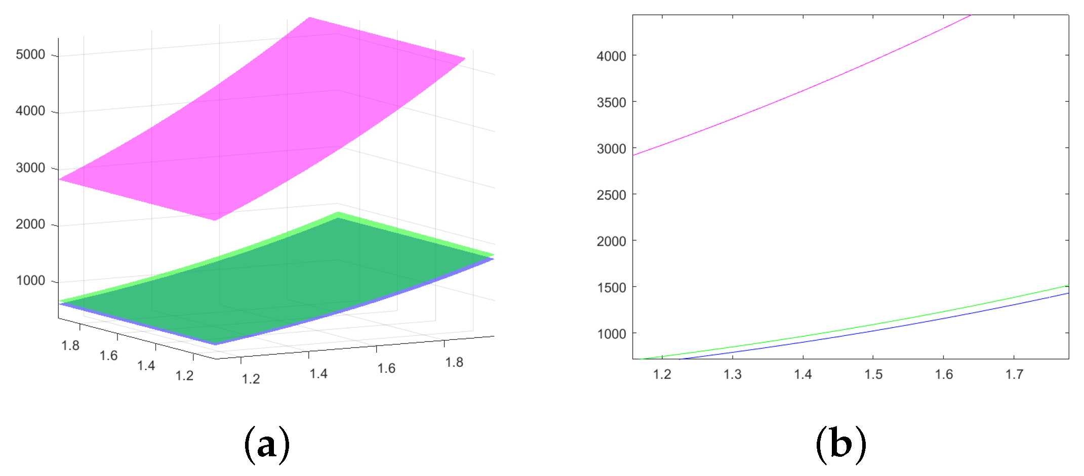
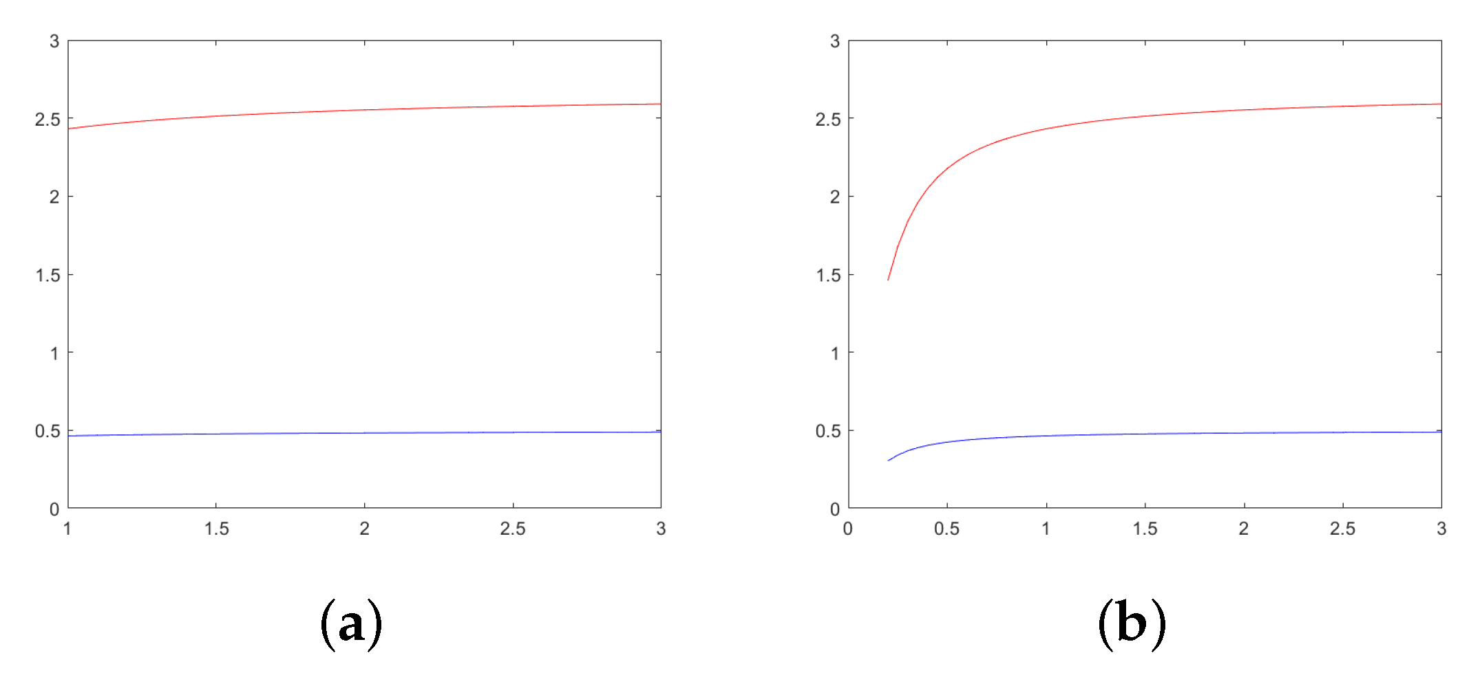
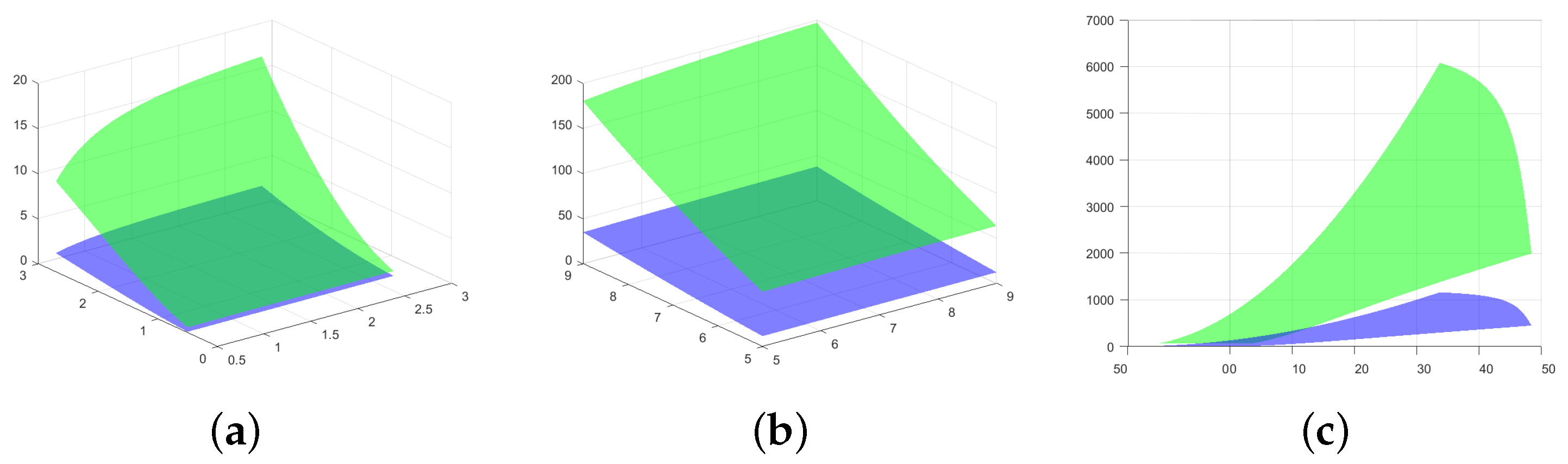
4. Visual Evaluation

The key findings of our study are illustrated graphically in this section, providing significant context for understanding the theoretical outcomes. In these examples, we consider functions similar to those in [6,8] because new results can be better analyzed together in a further study and compared. Analogous graphical evaluations are often presented in papers, such as in [43,44,45,46,47].

Example 1. 

We consider the function $f:[{\nu }_1,{\nu }_2]\to R$, $f\left(\eta \right)={(\eta +a_1)}^5$, ${\nu }_1=1,{\nu }_2=4$, and $z_1=2,$ $z_2=3.$ In addition, $\varphi \left(\eta \right)=\eta$ and $\sigma \left(0\right)=1,$ $w=0,k=1,\sigma \left(0\right)=1.$ It can be seen that the hypotheses of Theorem 2, page 4, and of Remark 8, page 6, are satisfied because we consider $w=0,k=1;$ therefore, the corresponding inequality holds and is as follows:

$$\begin{array}{cc}\hfill & f\left({\nu }_1+{\nu }_2-{\displaystyle \frac{z_1+z_2}{2}}\right)\hfill \\ & \le {\displaystyle \frac{2^{\vartheta -1}\Gamma (\vartheta +1)}{{(z_2-z_1)}^{\vartheta }}}\left[I_{{({\nu }_1+{\nu }_2-z_2)}^{+}}^{\vartheta }f\left({\nu }_1+{\nu }_2-{\displaystyle \frac{z_1+z_2}{2}}\right)+I_{{({\nu }_1+{\nu }_2-z_1)}^{-}}^{\vartheta }f\left({\nu }_1+{\nu }_2-{\displaystyle \frac{z_1+z_2}{2}}\right)\right]\hfill \\ & \le f\left({\nu }_1\right)+f\left({\nu }_2\right)-{\displaystyle \frac{f\left(z_1\right)+f\left(z_2\right)}{2}},\hfill \end{array}$$

and in this case, will be as follows:

$$\begin{array}{cc}\hfill & f\left({\displaystyle \frac{5}{2}}\right)\le 2^{\vartheta -1}\Gamma (\vartheta +1)[I_{2^{+}}^{\vartheta }f\left({\displaystyle \frac{5}{2}}\right)+I_{3^{-}}^{\vartheta }f\left({\displaystyle \frac{5}{2}}\right)]\le f\left(1\right)+f\left(4\right)-{\displaystyle \frac{f\left(2\right)+f\left(3\right)}{2}},\hfill \end{array}$$

or, by calculus,

$$\begin{array}{cc}\hfill & {({\displaystyle \frac{5}{2}}+a_1)}^5\le \vartheta 2^{\vartheta -1}\left[{\int }_2^{{\displaystyle \frac{5}{2}}}{({\displaystyle \frac{5}{2}}-\lambda )}^{\vartheta -1}{(\lambda +a_1)}^{5}d\lambda +{\int }_{{\displaystyle \frac{5}{2}}}^3{(\lambda -{\displaystyle \frac{5}{2}})}^{\vartheta -1}{(\lambda +a_1)}^{5}d\lambda \right]\hfill \\ & \le {(1+a_1)}^5+{(4+a_1)}^5-{\displaystyle \frac{{(2+a_1)}^5+{(3+a_1)}^5}{2}},\hfill \end{array}$$

which leads to the following:

$$\begin{array}{cc}\hfill & {({\displaystyle \frac{5}{2}}+a_1)}^5\le \vartheta ({\displaystyle \frac{5}{2}}+a_1)\left[{\displaystyle \frac{5}{16(\vartheta +4)}}+{\displaystyle \frac{5{(\frac{5}{2}+a_1)}^2}{2(\vartheta +2)}}+{\displaystyle \frac{{(\frac{5}{2}+a_1)}^4}{\vartheta }}\right]\hfill \\ & \le {(1+a_1)}^5+{(4+a_1)}^5-{\displaystyle \frac{{(2+a_1)}^5+{(3+a_1)}^5}{2}},\hfill \end{array}$$

In Figure 1a, three surfaces, which represent the left, middle, and right members of the inequalities from Theorem 2, page 4, and Remark 8, page 6, are graphically illustrated in the particular case of the previous example, when $\vartheta ,k\in [1,2]$. The left member, $M_s$, is the blue surface, the right member, $M_d$, is the magenta surface, and the middle member is the green surface. In Figure 1b, the same members of the same inequality from Figure 1a are represented, but when $\nu =1$ and $\vartheta \in [1,2]$. We also use the MATLAB R2023b software version for these figures.

Figure 1. (a) The graphs of three surfaces—the surface of the left member (graph in blue), the surface of the right member (graph in magenta), and the middle member (graph in green) of the inequality from Remark 8 are presented for the function $f\left(\eta \right)={(\eta +a_1)}^5$, $\psi \left(\eta \right)=\eta$, ${\nu }_1=1,{\nu }_2=4,z_1=2,z_2=3$ and $a_1,\vartheta \in [1,2]$; (b) the same three members of the same inequality from Figure 1a are represented, but when $\vartheta =1.5$ and $a_1\in [1,2]$.

Example 2. 

We consider the same function $f:[{\nu }_1,{\nu }_2]\to R$, $f\left(\eta \right)={\eta }^2$ and $z_1=2,$ $z_2=3$, like before. In addition, $\psi \left(\eta \right)=\eta$ and $\sigma \left(0\right)=1,$ $w=0$ are also like in the previous example. It can be seen that the hypotheses of Theorem 3 and of Theorem 3.5 from [33], see Remark 21, are satisfied; therefore, the corresponding inequality holds in this case:

$$|{\displaystyle \frac{f({\nu }_1+{\nu }_2-z_2)+f({\nu }_1+{\nu }_2-z_1)}{2}}-2^{{\displaystyle \frac{\alpha }{k}}-1}{\displaystyle \frac{{\Gamma }_k(\alpha +k)}{{(z_2-z_1)}^{\frac{\alpha }{k}}}}[\left({}_k\mathcal{J}_{{\left({\psi }^{-1}({\nu }_1+{\nu }_2-z_2)\right)}^{+}}^{\alpha ;\psi }\right)f({\nu }_1+{\nu }_2-{\displaystyle \frac{z_1+z_2}{2}})$$

$$+\left({}_k\mathcal{J}_{{\left({\psi }^{-1}({\nu }_1+{\nu }_2-z_1)\right)}^{-}}^{\alpha ;\psi }\right)f({\nu }_1+{\nu }_2-{\displaystyle \frac{z_1+z_2}{2}})\left]\right|\le {\displaystyle \frac{(z_2-z_1)}{2(\frac{\alpha }{k}+1)}}\left\{\right|f^{\prime }\left({\nu }_1\right)|+|f^{\prime }\left({\nu }_2\right)|-{\displaystyle \frac{|f^{\prime }\left(z_1\right)|+|f^{\prime }\left(z_2\right)|}{2}}\}$$

The left member is as follows:

$$M_s=|{\displaystyle \frac{f\left(2\right)+f\left(3\right)}{2}}-2^{{\displaystyle \frac{\alpha }{k}}-1}{\Gamma }_k(\alpha +k)[\left({}_k\mathcal{J}_{{\left({\psi }^{-1}\left(2\right)\right)}^{+}}^{\alpha ;\psi }\right)f(5-{\displaystyle \frac{5}{2}})+\left({}_k\mathcal{J}_{{\left({\psi }^{-1}\left(3\right)\right)}^{-}}^{\alpha ;\psi }\right)f(5-{\displaystyle \frac{5}{2}})]|$$

$$=|{\displaystyle \frac{13}{2}}-2^{{\displaystyle \frac{\alpha }{k}}-1}\alpha {\Gamma }_k\left(\alpha \right)[\left({}_k\mathcal{J}_{2^{+}}^{\alpha ;\psi }\right)f\left({\displaystyle \frac{5}{2}}\right)+\left({}_k\mathcal{J}_{3^{-}}^{\alpha ;\psi }\right)f\left({\displaystyle \frac{5}{2}}\right)]|$$

$$=|{\displaystyle \frac{13}{2}}-2^{{\displaystyle \frac{\alpha }{k}}-1}{\displaystyle \frac{\alpha }{k}}[{\int }_2^{{\displaystyle \frac{5}{2}}}{({\displaystyle \frac{5}{2}}-\lambda )}^{{\displaystyle \frac{\alpha }{k}}-1}{\lambda }^{2}d\lambda +{\int }_{{\displaystyle \frac{5}{2}}}^3{(\lambda -{\displaystyle \frac{5}{2}})}^{{\displaystyle \frac{\alpha }{k}}-1}{\lambda }^{2}d\lambda ]|.$$

By calculus, we have the following:

$$M_s=|{\displaystyle \frac{13}{2}}-{\displaystyle \frac{\alpha }{4}}({\displaystyle \frac{25}{\alpha }}+{\displaystyle \frac{1}{\alpha +2k}})|.$$

The right member is as follows:

$$M_d={\displaystyle \frac{1}{2(\frac{\alpha }{k}+1)}}5.$$

In Figure 2a, two surfaces that represent the left and right members of the inequalities from Theorem 3 are graphically illustrated in the particular case of the previous example, when $\alpha ,k\in [0.01,2.6]$. The left member, $M_s$, is the blue surface, and the right member, $M_d$, is the magenta surface. In Figure 2b, the same members of the same inequality from Figure 2a are represented, but when $k=1$ and $\alpha \in [0.01,6]$; in Figure 2c, the blue graphic represents the left member of the inequality from Theorem 3, and the magenta graphic represents the right member, but when $\alpha =5$ and $k\in [0.01,6]$. We used the MATLAB R2023b software version for these figures.

Figure 2. (a) The graphs of two surfaces—the surface of the left member (graph in blue) and the surface of the right member (graph in magenta) of the inequality from Theorem 3 are presented for the function $f\left(\eta \right)={\eta }^2$, $\psi \left(\eta \right)=\eta$, ${\nu }_1=1,{\nu }_2=4,z_1=2,z_2=3$ and $\alpha ,k\in [0.001,2.6]$ from the previous example; (b) the same members of the same inequality from Figure 2a are presented, but when $k=1$ and $\alpha \in [0.01,6]$; (c) the blue graphic represents the left member of the inequality from Theorem 3, and the magenta graphic represents the right member, but when $\alpha =5$ and $k\in [0.01,6]$.

Example 3. 

We consider the function $f:[{\nu }_1,{\nu }_2]\to R$, $f\left(\eta \right)={\eta }^2$, ${\nu }_1=1,{\nu }_2=6$ and $z_1=2,$ $z_2=4.$ In addition, $\psi \left(\eta \right)=\eta$ and $w=1,\sigma \left(j\right)=1,\rho =1,\nu =2k.$ It can be seen that the hypothesis of Theorem 3, page 8, is satisfied; therefore, we consider the corresponding inequality:

$$\begin{array}{cc}\hfill & |{\displaystyle \frac{f\left({\nu }_1+{\nu }_2-z_2\right)+f\left({\nu }_1+{\nu }_2-z_1\right)}{2}}-{\displaystyle \frac{2^{\frac{\nu }{k}-1}}{k{(z_2-z_1)}^{\frac{\nu }{k}}{}_k\mathcal{F}_{\rho ,\vartheta +k}^{\sigma }\left[w{\left(\frac{z_2-z_1}{2}\right)}^{\rho }\right]}}\times \hfill \\ & \times [{}_k{}^{\psi }\mathcal{J}_{\rho ,\nu ,{\psi }^{-1}{({\nu }_1+{\nu }_2-z_2)}^{+};w}^{\sigma }\left(fo\psi \right)\left({\psi }^{-1}({\nu }_1+{\nu }_2-{\displaystyle \frac{z_1+z_2}{2}})\right)\hfill \\ & +{}_k{}^{\psi }\mathcal{J}_{\rho ,\nu ,{\psi }^{-1}{({\nu }_1+{\nu }_2-z_1)}^{-};w}^{\sigma }\left(fo\psi \right)\left({\psi }^{-1}({\nu }_1+{\nu }_2-{\displaystyle \frac{z_1+z_2}{2}})\right)\left]\right|\hfill \\ & \le {\displaystyle \frac{k(z_2-z_1){}_k\mathcal{F}_{\rho ,\nu +2k}^{\sigma }\left[w{\left(\frac{z_2-z_1}{2}\right)}^{\rho }\right]}{2{}_k\mathcal{F}_{\rho ,\nu +k}^{\sigma }\left[w{\left(\frac{z_2-z_1}{2}\right)}^{\rho }\right]}}\left[\right|f^{\prime }\left({\nu }_1\right)|+|f^{\prime }\left({\nu }_2\right)|-{\displaystyle \frac{|f^{\prime }\left(z_1\right)|+|f^{\prime }\left(z_2\right)|}{2}}].\hfill \end{array}$$

We denote the following:

$$\begin{array}{cc}\hfill & J_1={}_k{}^{\psi }\mathcal{J}_{\rho ,\nu ,{\psi }^{-1}{({\nu }_1+{\nu }_2-z_2)}^{+};w}^{\sigma }\left(fo\psi \right)\left({\psi }^{-1}({\nu }_1+{\nu }_2-{\displaystyle \frac{z_1+z_2}{2}})\right)={}_k{}^{\psi }\mathcal{J}_{1,2k,3^{+};1}^{1}f\left(4\right)\hfill \\ & ={\int }_3^4(4-\eta ){}_k\mathcal{F}_{\rho ,\nu }^{\sigma }\left[{(4-\eta )}^{\rho }\right]{\eta }^{2}d\eta \hfill \\ & ={\displaystyle \frac{1}{k}}{\int }_3^4(e^{{\displaystyle \frac{4-\eta }{k}}}-1){\eta }^{2}d\eta =9e^{{\displaystyle \frac{1}{k}}}-16+2k(3e^{{\displaystyle \frac{1}{k}}}-4)+2k^2(e^{{\displaystyle \frac{1}{k}}}-1)-{\displaystyle \frac{37}{3k}},\hfill \end{array}$$

and

$$\begin{array}{cc}\hfill & J_2={}_k{}^{\psi }\mathcal{J}_{\rho ,\nu ,{\psi }^{-1}{({\nu }_1+{\nu }_2-z_1)}^{-};w}^{\sigma }\left(fo\psi \right)\left({\psi }^{-1}({\nu }_1+{\nu }_2-{\displaystyle \frac{z_1+z_2}{2}})\right)={}_k{}^{\psi }\mathcal{J}_{1,2k,5^{-};1}^{1}f\left(4\right)\hfill \\ & ={\int }_4^5(\eta -4){}_k\mathcal{F}_{\rho ,\nu }^{\sigma }\left[{(\eta -4)}^{\rho }\right]f\left(\eta \right)d\eta \hfill \\ & ={\displaystyle \frac{1}{k}}{\int }_4^5(e^{{\displaystyle \frac{\eta -4}{k}}}-1){\eta }^{2}d\eta =25e^{{\displaystyle \frac{1}{k}}}-16-k(10e^{{\displaystyle \frac{1}{k}}}-8)+2k^2(e^{{\displaystyle \frac{1}{k}}}-1)-{\displaystyle \frac{61}{3k}}.\hfill \end{array}$$

It was previously established that

$${}_k\mathcal{F}_{1,2k}^1[4-\eta ]=\sum _{j=0}^{\infty }{\displaystyle \frac{1}{k{\Gamma }_k(jk+2k)}}{(4-\eta )}^j={\displaystyle \frac{1}{k(4-\eta )}}(e^{{\displaystyle \frac{4-\eta }{k}}}-1).$$

Therefore, we have the following:

$$\begin{array}{cc}\hfill & M_s=|{\displaystyle \frac{f\left(3\right)+f\left(5\right)}{2}}-{\displaystyle \frac{1}{2k{}_k\mathcal{F}_{1,3k}^1\left[1\right]}}[{}_k{}^{\psi }\mathcal{J}_{1,2k,3^{+};1}^{1}f\left(4\right)+{}_k{}^{\psi }\mathcal{J}_{1,2k,5^{-};1}^{1}f\left(4\right)]|\hfill \\ & =|17-{\displaystyle \frac{1}{2k}}{\displaystyle \frac{1}{(e^{\frac{1}{k}}-1-\frac{1}{k})\frac{1}{k}}}[J_1+J_2]|=|17-{\displaystyle \frac{1}{e^{\frac{1}{k}}-1-\frac{1}{k}}}[17e^{{\displaystyle \frac{1}{k}}}-16-2k{e}^{{\displaystyle \frac{1}{k}}}+2k^2{e}^{{\displaystyle \frac{1}{k}}}-2k^2-{\displaystyle \frac{49}{3k}}]|\hfill \end{array}$$

and

$$\begin{array}{cc}\hfill & M_d={\displaystyle \frac{2k{}_k\mathcal{F}_{1,4k}^1\left[1\right]}{2{}_k\mathcal{F}_{1,3k}^1\left[1\right]}}\left[\right|f^{\prime }\left(1\right)|+|f^{\prime }\left(6\right)|-{\displaystyle \frac{|f^{\prime }\left(2\right)|+|f^{\prime }\left(4\right)|}{2}}]={\displaystyle \frac{8k(e^{\frac{1}{k}}-1-\frac{1}{k}-\frac{1}{2k^2})}{e^{\frac{1}{k}}-1-\frac{1}{k}}}.\hfill \end{array}$$

We also have that

$${}_k\mathcal{F}_{1,3k}^1\left[1\right]=\sum _{j=0}^{\infty }{\displaystyle \frac{1}{k^{j+3}\Gamma (j+3)}}={\displaystyle \frac{1}{k}}(e^{{\displaystyle \frac{1}{k}}}-1-{\displaystyle \frac{1}{k}}).$$

In Figure 3a, two surfaces, which represent the left and the right members of the inequalities from Theorem 3, page 8, are graphically illustrated in this particular case of this example when $k\in [1,3]$. The left member, $M_s$, is the blue line, and the right member, $M_d$, is the red line. In Figure 3b, the same members of the same inequality from Figure 3a are represented, but when $\vartheta \in [0.2,3]$. MATLAB R2023b software version was used for all these figures.

Figure 3. (a) The graphs of the left-hand side (graph in blue) and the right-hand side (graph in red) of the inequality from Theorem 3, page 8, are presented for the function $f\left(\eta \right)={\eta }^2$, $\psi \left(\eta \right)=\eta$, ${\nu }_1=1,{\nu }_2=6$, $z_1=2,z_2=4,w=1$, $\rho =1,\sigma \left(j\right)=1,\nu =2k$, and $k\in [1,3]$; (b) the same two members of the same inequality from Figure 3a are represented, but when $\vartheta \in [0.2,3]$.

Example 4. 

We consider the function $f:[{\nu }_1,{\nu }_2]\to R$, $f\left(\eta \right)={\eta }^2$, ${\nu }_1=l,{\nu }_2=6l$ and $z_1=2l,$ $z_2=4l.$ In addition, $\psi \left(\eta \right)=\eta$ and $w=1,\sigma \left(j\right)=1,\rho =1,\nu =2k,k>0.$ It can be seen that the hypothesis of Theorem 3, page 8, is fulfilled; therefore, we shall consider the following inequality:

$$|{\displaystyle \frac{f\left(3l\right)+f\left(5l\right)}{2}}-{\displaystyle \frac{2}{4k{l}^2{}_k\mathcal{F}_{1,3k}^1\left[l\right]}}[{}_k{}^{\psi }\mathcal{J}_{1,2k,{3l}^{+};1}f\left(4l\right)+{}_k{}^{\psi }\mathcal{J}_{1,2k,{5l}^{-};1}f\left(4l\right)]|\le$$

$$\le {\displaystyle \frac{2kl{}_k\mathcal{F}_{1,4k}^1\left[l\right]}{2{}_k\mathcal{F}_{1,3k}^1\left[l\right]}}\left[\right|f^{\prime }\left(l\right)|+|f^{\prime }\left(6l\right)|-{\displaystyle \frac{|f^{\prime }\left(2l\right)|+|f^{\prime }\left(4l\right)|}{2}}].$$

Using analogous calculus, the left member, $M_s$, is as follows:

$$M_s=|17l^2-{\displaystyle \frac{1}{2(e^{\frac{l}{k}}-1-\frac{l}{k})}}[J_1+J_2]|,$$

where

$$J_1=l^2(9e^{{\displaystyle \frac{l}{k}}}-16)+2kl(3e^{{\displaystyle \frac{l}{k}}}-4)+2k^2(e^{{\displaystyle \frac{l}{k}}}-1)-{\displaystyle \frac{37l^3}{3k}}$$

and

$$J_2=l^2(25e^{{\displaystyle \frac{l}{k}}}-16)-2kl(5e^{{\displaystyle \frac{l}{k}}}-4)+2k^2(e^{{\displaystyle \frac{l}{k}}}-1)-{\displaystyle \frac{61l^3}{3k}}.$$

The right member, $M_d$, will be as follows:

$$M_d=8kl{\displaystyle \frac{e^{\frac{l}{k}}-1-\frac{l}{k}-\frac{l^2}{2k^2}}{e^{\frac{l}{k}}-1-\frac{l}{k}}}.$$

In Figure 4, the graphic displays the surface representing the left-hand side in blue and the right-hand side in green, using the previously mentioned function and parameters. For Figure 4a, we consider $l,k\in [0.5,2.7]$, for Figure 4b, we take $l,k\in [5,9]$, and for Figure 4c, we have $l,k\in [5,50]$.

Figure 4. (a) The graphs of the left-hand side (surface in blue) and the right-hand side (surface in green) of the inequality from Theorem 3, page 8, are presented for the function $f\left(\eta \right)={\eta }^2$, $\psi \left(\eta \right)=\eta$, ${\nu }_1=l,{\nu }_2=6l$, $z_1=2l,z_2=4l,w=1$, $\rho =1,\sigma \left(j\right)=1,\nu =2k$ and $l,k\in [0.5,2.7]$; (b) the same two members of the same inequality from Figure 4a are represented, but when $l,k\in [5,9]$; (c) the same two members of the same inequality from Figure 4a are represented when parameters $l,k\in [5,50]$, but the figure is rotated.

5. Applications

Finally, we address some novel applications of our results to the modified Bessel functions and q-digamma function.

5.1. Modified Bessel Function

Let ${\Im }_{\lambda }:R\to (0,1]$ be defined by the following:

$${\Im }_{\lambda }\left(\theta \right)=2^{\lambda }\Gamma (1+\lambda ){\theta }^{-s}{I}_{\lambda }\left(\theta \right).$$

For this, we retrospect the representation of modified Bessel functions, which is given, as detailed in [48]:

$${\Im }_{\lambda }\left(\theta \right)=\sum _{u=0}^{\infty }{\displaystyle \frac{{\left(\frac{\theta }{2}\right)}^{\lambda +2u}}{u!\Gamma (\lambda +u+1)}},$$

The first and nth-order derivative formula’s ${\Im }_{\lambda }\left(\theta \right)$, which are given as detailed in [49]:

$${\Im }_{\lambda }^{\prime }\left(\theta \right)={\displaystyle \frac{\theta }{2(1+\lambda )}}{\Im }_{\lambda +1}\left(\theta \right),$$

$$\begin{array}{c}\hfill {\displaystyle \frac{{\partial }^n{\Im }_{\lambda }\left(\theta \right)}{\partial {\theta }^n}}=2^{n-2\lambda }\sqrt{\pi }{\theta }^{\lambda -n}\Gamma (1+\lambda ){}_{2}F_3\left({\displaystyle \frac{1+\lambda }{2}},{\displaystyle \frac{2+\lambda }{2}};{\displaystyle \frac{1+\lambda -n}{2}},{\displaystyle \frac{2+\lambda -n}{2}},1+\lambda ;{\displaystyle \frac{{\theta }^2}{4}}\right),\end{array}$$

where ${}_{2}F_3(.,.;.,.,.;.)$ is the hypergeometric function defined by the following [49]:

$$\begin{array}{c}\hfill {}_{2}F_3\left({\displaystyle \frac{1+\lambda }{2}},{\displaystyle \frac{2+\lambda }{2}};{\displaystyle \frac{1+\lambda -n}{2}},{\displaystyle \frac{2+\lambda -n}{2}},1+\lambda ;{\displaystyle \frac{{\theta }^2}{4}}\right)=\sum _{r=0}^{\infty }{\displaystyle \frac{{\left(\frac{1+\lambda }{2}\right)}_r{\left(\frac{2+\lambda }{2}\right)}_r{\theta }^{2r}}{{\left(\frac{1+\lambda -n}{2}\right)}_r{\left(\frac{2+\lambda -n}{2}\right)}_r{(1+\lambda )}_r{4}^{r}r!}}.\end{array}$$

Proposition 1. 

Let $0<{\nu }_1<{\nu }_2$ and $\lambda \ge 1.$ Then, for all $z_1,z_2\in [{\nu }_1,{\nu }_2]$ that are real numbers, we have the following:

$$\begin{array}{cc}\hfill & |{\displaystyle \frac{({\nu }_1+{\nu }_2-z_2){\Im }_{\lambda +1}({\nu }_1+{\nu }_2-z_2)+({\nu }_1+{\nu }_2-z_1){\Im }_{\lambda +1}({\nu }_1+{\nu }_2-z_1)}{4(1+\lambda )}}\hfill \\ & -{\displaystyle \frac{{\Im }_{\lambda }({\nu }_1+{\nu }_2-z_1)-{\Im }_{\lambda }({\nu }_1+{\nu }_2-z_2)}{z_2-z_1}}|\hfill \\ & \le {\displaystyle \frac{z_2-z_1}{2^{2\lambda -1}}}\sqrt{\pi }\Gamma (1+\lambda )\times \hfill \\ \hfill & \times [2{\nu }_1^{\lambda -2}{}_{2}F_3\left({\displaystyle \frac{1+\lambda }{2}},{\displaystyle \frac{2+\lambda }{2}};{\displaystyle \frac{\lambda -1}{2}},{\displaystyle \frac{\lambda }{2}},1+\lambda ;{\displaystyle \frac{{\nu }_1^2}{4}}\right)+2{\nu }_2^{\lambda -2}{}_{2}F_3\left({\displaystyle \frac{1+\lambda }{2}},{\displaystyle \frac{2+\lambda }{2}};{\displaystyle \frac{\lambda -1}{2}},{\displaystyle \frac{\lambda }{2}},1+\lambda ;{\displaystyle \frac{{\nu }_2^2}{4}}\right)\hfill \\ \hfill & -z_1^{\lambda -2}{}_{2}F_3\left({\displaystyle \frac{1+\lambda }{2}},{\displaystyle \frac{2+\lambda }{2}};{\displaystyle \frac{\lambda -1}{2}},{\displaystyle \frac{\lambda }{2}},1+\lambda ;{\displaystyle \frac{z_1^2}{4}}\right)-z_2^{\lambda -2}{}_{2}F_3\left({\displaystyle \frac{1+\lambda }{2}},{\displaystyle \frac{2+\lambda }{2}};{\displaystyle \frac{\lambda -1}{2}},{\displaystyle \frac{\lambda }{2}},1+\lambda ;{\displaystyle \frac{z_2^2}{4}}\right)].\hfill \end{array}$$

Proof. 

The proof is derived directly from Theorem 3, considering $f\left(\eta \right)={\Im }_{\lambda }^{\prime }\left(\eta \right),$ $\vartheta =k=1,$ $j=0,$ $\psi \left(\eta \right)=\eta$ and the fact that $\sigma \left(0\right)=1$. □

Proposition 2. 

Let $0<{\nu }_1<{\nu }_2$ and $\lambda \ge 1.$ Then, for all $z_1,z_2\in [{\nu }_1,{\nu }_2]$ that are real numbers, we have the following:

$$\begin{array}{cc}\hfill & |{\displaystyle \frac{({\nu }_1+{\nu }_2-z_2){\Im }_{\lambda +1}({\nu }_1+{\nu }_2-z_2)+({\nu }_1+{\nu }_2-z_1){\Im }_{\lambda +1}({\nu }_1+{\nu }_2-z_1)}{4(1+\lambda )}}\hfill \\ & -{\displaystyle \frac{{\Im }_{\lambda }({\nu }_1+{\nu }_2-z_1)-{\Im }_{\lambda }({\nu }_1+{\nu }_2-z_2)}{z_2-z_1}}|\hfill \\ & \le {\displaystyle \frac{{(z_2-z_1)}^2}{{3.2}^{2\lambda }}}\sqrt{\pi }\Gamma (1+\lambda )[2{\nu }_1^{\lambda -3}{}_{2}F_3\left({\displaystyle \frac{1+\lambda }{2}},{\displaystyle \frac{2+\lambda }{2}};{\displaystyle \frac{\lambda -2}{2}},{\displaystyle \frac{\lambda -1}{2}},1+\lambda ;{\displaystyle \frac{{\nu }_1^2}{4}}\right)\hfill \\ & +2{\nu }_2^{\lambda -3}{}_{2}F_3\left({\displaystyle \frac{1+\lambda }{2}},{\displaystyle \frac{2+\lambda }{2}};{\displaystyle \frac{\lambda -2}{2}},{\displaystyle \frac{\lambda -1}{2}},1+\lambda ;{\displaystyle \frac{{\nu }_2^2}{4}}\right)\hfill \\ & -z_1^{\lambda -3}{}_{2}F_3\left({\displaystyle \frac{1+\lambda }{2}},{\displaystyle \frac{2+\lambda }{2}};{\displaystyle \frac{\lambda -2}{2}},{\displaystyle \frac{\lambda -1}{2}},1+\lambda ;{\displaystyle \frac{z_1^2}{4}}\right)\hfill \\ & -z_2^{\lambda -3}{}_{2}F_3\left({\displaystyle \frac{1+\lambda }{2}},{\displaystyle \frac{2+\lambda }{2}};{\displaystyle \frac{\lambda -2}{2}},{\displaystyle \frac{\lambda -1}{2}},1+\lambda ;{\displaystyle \frac{z_2^2}{4}}\right)].\hfill \end{array}$$

Proof. 

The proof is derived directly from Theorem 6, considering $f\left(\eta \right)={\Im }_{\lambda }^{\prime }\left(\eta \right),$ $\vartheta =k=1,$ $j=0,$ $\psi \left(\eta \right)=\eta$ and the fact that $\sigma \left(0\right)=1$. □

Remark 26. 

We can obtain additional inequalities for the modified Bessel function of the first kind by using the same approach as in Propositions 1 and 2. Here, we omit their proofs, and the details are left to the interested reader.

5.2. q-Digamma Function

Here, we revisit the notion of the q-digamma function and its mathematical representations; assume that $0<q<1.$ The q-digamma function ${\chi }_q\left(u\right)$ (for further information, refer to [20]) can be expressed as follows:

$$\begin{array}{cc}\hfill {\chi }_q\left(u\right)& =-ln(1-q)+ln\left(q\right)\sum _{i=0}^{\infty }{\displaystyle \frac{q^{i+u}}{1-q^{i+u}}}\hfill \\ & =-ln(1-q)+ln\left(q\right)\sum _{i=0}^{\infty }{\displaystyle \frac{q^{iu}}{1-q^{iu}}}.\hfill \end{array}$$

If $q>1$ and $u>1,$ the q-digamma function ${\chi }_q\left(u\right)$ can be represented as follows:

$$\begin{array}{cc}\hfill {\chi }_q\left(u\right)& =-ln(q-1)+ln\left(q\right)[u-{\displaystyle \frac{1}{2}}-\sum _{i=0}^{\infty }{\displaystyle \frac{q^{-(i+u)}}{1-q^{-(i+u)}}}]\hfill \\ & =-ln(q-1)+ln\left(q\right)[u-{\displaystyle \frac{1}{2}}-\sum _{i=0}^{\infty }{\displaystyle \frac{q^{-iu}}{1-q^{-iu}}}].\hfill \end{array}$$

The notion briefed above shows that for $q>0,$ the function ${\chi }_q^{\prime }\left(u\right)$ is completely monotonic on the interval $(0,\infty )$, which implies that it is a convex mapping. From these facts, we can formulate the following important findings concerning the q-digamma function.

Proposition 3. 

From Theorem 2, we acquire the following:

$$\begin{array}{cc}\hfill & {\chi }_q^{\prime }\left({\nu }_1+{\nu }_2-{\displaystyle \frac{z_1+z_2}{2}}\right)\hfill \\ & \le {\displaystyle \frac{1}{z_2-z_1}}\left[{\chi }_q({\nu }_1+{\nu }_2-z_1)-{\chi }_q({\nu }_1+{\nu }_2-z_2)\right]\le {\chi }_q^{\prime }\left({\nu }_1\right)+{\chi }_q^{\prime }\left({\nu }_2\right)-{\displaystyle \frac{{\chi }_q^{\prime }\left(z_1\right)+{\chi }_q^{\prime }\left(z_2\right)}{2}}.\hfill \end{array}$$

Proof. 

The proof is derived directly from Theorem 2, considering $f\left(\eta \right)={\chi }_q^{\prime }\left(\eta \right),$ $\vartheta =k=1,$ $j=0,$ $\psi \left(\eta \right)=\eta$ and the fact that $\sigma \left(0\right)=1$. □

Remark 27. 

If we set $z_1={\nu }_1$ and $z_2={\nu }_2$ in Proposition 3, then Proposition 3 reduces to inequality (19) of [35] (Example 3).

Proposition 4. 

From Theorem 3, we acquire the following:

$$\begin{array}{cc}\hfill & |{\displaystyle \frac{{\chi }_q^{\prime }({\nu }_1+{\nu }_2-z_2)+{\chi }_q^{\prime }({\nu }_1+{\nu }_2-z_1)}{2}}-{\displaystyle \frac{1}{z_2-z_1}}\left[{\chi }_q({\nu }_1+{\nu }_2-z_1)-{\chi }_q({\nu }_1+{\nu }_2-z_2)\right]|\hfill \\ & \le (z_2-z_1)\left[{\chi }_q^{″}\left({\nu }_1\right)+{\chi }_q^{″}\left({\nu }_2\right)-{\displaystyle \frac{{\chi }_q^{″}\left(z_1\right)+{\chi }_q^{″}\left(z_2\right)}{2}}\right].\hfill \end{array}$$

Proof. 

The proof is derived directly from Theorem 3, considering $f\left(\eta \right)={\chi }_q^{\prime }\left(\eta \right),$ $\vartheta =k=1,$ $j=0,$ $\psi \left(\eta \right)=\eta$ and the fact that $\sigma \left(0\right)=1$. □

Proposition 5. 

From Theorem 4, we acquire the following:

$$\begin{array}{cc}\hfill & |{\displaystyle \frac{{\chi }_q^{\prime }({\nu }_1+{\nu }_2-z_2)+{\chi }_q^{\prime }({\nu }_1+{\nu }_2-z_1)}{2}}-{\displaystyle \frac{1}{z_2-z_1}}\left[{\chi }_q({\nu }_1+{\nu }_2-z_1)-{\chi }_q({\nu }_1+{\nu }_2-z_2)\right]|\hfill \\ & \le {\displaystyle \frac{(z_2-z_1)}{4\sqrt[p]{1+p}}}[{\left(|{\chi }_q^{″}\left({\nu }_1\right){|}^q+{\left|{\chi }_q^{″}\left({\nu }_2\right)\right|}^q-{\displaystyle \frac{|{\chi }_q^{″}\left(z_1\right){|}^q+3{\left|{\chi }_q^{″}\left(z_2\right)\right|}^q}{4}}\right)}^{{\displaystyle \frac{1}{q}}}\hfill \\ & +{\left(|{\chi }_q^{″}\left({\nu }_1\right){|}^q+{\left|{\chi }_q^{″}\left({\nu }_2\right)\right|}^q-{\displaystyle \frac{3|{\chi }_q^{″}\left(z_1\right){|}^q+{\left|{\chi }_q^{″}\left(z_2\right)\right|}^q}{4}}\right)}^{{\displaystyle \frac{1}{q}}}].\hfill \end{array}$$

Proof. 

The proof is derived directly from Theorem 4, considering $f\left(\eta \right)={\chi }_q^{\prime }\left(\eta \right),$ $\vartheta =k=1,$ $j=0,$ $\psi \left(\eta \right)=\eta$ and the fact that $\sigma \left(0\right)=1$. □

Proposition 6. 

From Theorem 5, we acquire the following:

$$\begin{array}{cc}\hfill & |{\displaystyle \frac{{\chi }_q^{\prime }({\nu }_1+{\nu }_2-z_2)+{\chi }_q^{\prime }({\nu }_1+{\nu }_2-z_1)}{2}}-{\displaystyle \frac{1}{z_2-z_1}}\left[{\chi }_q({\nu }_1+{\nu }_2-z_1)-{\chi }_q({\nu }_1+{\nu }_2-z_2)\right]|\hfill \\ & \le {\displaystyle \frac{(z_2-z_1)}{2}}[{\left(|{\chi }_q^{″}\left({\nu }_1\right){|}^q+{\left|{\chi }_q^{″}\left({\nu }_2\right)\right|}^q-{\displaystyle \frac{|{\chi }_q^{″}\left(z_1\right){|}^q+5{\left|{\chi }_q^{″}\left(z_2\right)\right|}^q}{6}}\right)}^{{\displaystyle \frac{1}{q}}}\hfill \\ & +{\left(|{\chi }_q^{″}\left({\nu }_1\right){|}^q+{\left|{\chi }_q^{″}\left({\nu }_2\right)\right|}^q-{\displaystyle \frac{5|{\chi }_q^{″}\left(z_1\right){|}^q+{\left|{\chi }_q^{″}\left(z_2\right)\right|}^q}{6}}\right)}^{{\displaystyle \frac{1}{q}}}].\hfill \end{array}$$

Proof. 

The proof is derived directly from Theorem 5, considering $f\left(\eta \right)={\chi }_q^{\prime }\left(\eta \right),$ $\vartheta =k=1,$ $j=0,$ $\psi \left(\eta \right)=\eta$ and the fact that $\sigma \left(0\right)=1$. □

Remark 28. 

Applying our main results, we may derive a number of attractive inequalities related to the q-digamma function using the same method as in the relations that were previously demonstrated. Here, we do not include their proofs.

Remark 29. 

New refinements of inequalities, as presented in the application section of [30] and in Examples 1 and 3 from [35], could be provided by utilizing previous results obtained from the modified Bessel function and q-digamma function in further research.

6. Discussions and Conclusions

Many studies have been conducted to optimize the bounds utilizing numerous fractional integrals; ${\psi }_k$-RFI being extensively used to optimize bounds in the context of current developments in fractional analysis. Given the significance of this subject and its broad applications in modeling real-world phenomena, the main goal of this research is to develop new and generalized inequalities that utilize ${\psi }_k$-RFIs to connect the inequality theory and fractional analysis. Furthermore, we show how the findings, when examined in the context of integral inequalities, advance and expand upon existing research in this field.

This work continues the study that began in [8], focusing on H-H-M-type inequalities for ${\psi }_k$-RFIs. Two identities that are essential to demonstrating H-H-M inequalities for ${\psi }_k$-RFIs are presented in Lemma 1 for the corresponding Theorems 3–5 for functions whose first derivatives in the modulus are convex. Moreover, Lemma 2 is used in the proofs of Theorems 6–8.

Our investigation concludes that the main advantage of these new H-H-M-type inequalities is that ${\psi }_k$-RFI can be particularized so as to re-obtain several types of classical H-H-M inequalities for different fractional integrals. Examples and visual evaluations are provided using MATLAB R2023b software to validate the results; some applications are presented for the modified Bessel function and the q-digamma function.

These findings could inspire researchers who study fractional calculus to prove new results for different types of convexity. As the fractional order model becomes more significant in many domains, our inequalities extend the analytical approach that is essential for integral operator analysis and estimation techniques.

These contributions provide more precise and accurate approaches to solving real-world problems, making them useful for both researchers and professionals in the fields of fractional calculus, numerical analysis, and control theory. In probability theory and statistics, where convex functions frequently appear in the framework of probability distributions, cumulative distribution functions, and moments of random variables, these inequalities can be useful. As an illustration, consider the statistical properties of random variables.

We suggest that potential readers approach this article to obtain additional results by utilizing different fractional integrals and various types of convexity. Numerous applications can be developed for the new inequalities, including linear combinations of means, matrices, composite quadrature formulas, modified Bessel functions of the second kind, and novel parametric iterative schemes with a specific order of convergence. In addition, future studies could provide some iterative schemes using physical examples.

References

- Lakshmikantham, V. Differential and Integral Inequalities: Theory and Applications, Vol. I: Ordinary Differential Equations; Academic Press: Cambridge, MA, USA, 1969. [Google Scholar]
- Javed, M.Z.; Awan, M.U.; Bin-Mohsin, B.; Budak, H.; Dragomir, S.S. Some Classical Inequalities Associated with Generic Identity and Applications. Axioms 2024, 13, 533. [Google Scholar] [CrossRef]
- Walter, W. Differential and Integral Inequalities; Springer Science & Business Media: Berlin/Heidelberg, Germany, 2012; Volume 55. [Google Scholar]
- Zhu, C.; Fečkan, M.; Wang, J. Fractional Integral Inequalities for Differentiable Convex Mappings and Applications to Special Means and a Midpoint Formula. J. Appl. Math. Stat. Inform. 2012, 8, 21–28. [Google Scholar] [CrossRef]
- Denton, Z.; Vatsala, A.S. Fractional Integral Inequalities and Applications. Comput. Math. Appl. 2010, 59, 1087–1094. [Google Scholar] [CrossRef]
- Ciurdariu, L.; Grecu, E. Hermite–Hadamard–Mercer-Type Inequalities for Three-Times Differentiable Functions. Axioms 2024, 13, 413. [Google Scholar] [CrossRef]
- Kermausuor, S.; Nwaeze, E.R. Mathematical Inequalities in Fractional Calculus and Applications. Fractal Fract. 2024, 8, 471. [Google Scholar] [CrossRef]
- Hussain, T.; Ciurdariu, L.; Grecu, E. A New Inclusion on Inequalities of the Hermite–Hadamard–Mercer Type for Three-Times Differentiable Functions. Mathematics 2024, 12, 3711. [Google Scholar] [CrossRef]
- Rashid, S.; Abdeljawad, T.; Jarad, F.; Noor, M.A. Some Estimates for Generalized Riemann-Liouville Fractional Integrals of Exponentially Convex Functions and Their Applications. Mathematics 2019, 7, 807. [Google Scholar] [CrossRef]
- Hilfer, R. Applications of Fractional Calculus in Physics; World Scientific: Singapore, 2000. [Google Scholar]
- Baleanu, D.; Güvenç, Z.B.; Machado, J.T. New Trends in Nanotechnology and Fractional Calculus Applications; Springer: Berlin/Heidelberg, Germany, 2010; Volume 10. [Google Scholar]
- Atangana, A. Application of Fractional Calculus to Epidemiology; Fractional Dynamics; Walter de Gruyter: Warsaw, Poland, 2015; Volume 2015, pp. 174–190. [Google Scholar]
- Magin, R. Fractional Calculus in Bioengineering, part 1. Crit. Rev. Biomed. Eng. 2004, 32, 1. [Google Scholar]
- Monje, C.A.; Vinagre, B.M.; Feliu, V.; Chen, Y. Tuning and Auto-Tuning of Fractional Order Controllers for Industry Applications. Control Eng. Pract. 2008, 16, 798–812. [Google Scholar] [CrossRef]
- Dragomir, S.S. New Estimation of the Remainder in Taylor’s Formula using Grüss Type Inequalities and Applications. Math. Ineq. Appl. 1999, 2, 183–194. [Google Scholar] [CrossRef]
- Jensen, J.L.W.V. Sur les Fonctions Convexes et les Inégalités entre les Valeurs Moyennes. Acta Math. 1906, 30, 175–193. [Google Scholar]
- Hadamard, J. Étude sur les Propriétés des Fonctions entières et en particulier d’une Fonction considérée par Riemann. J. Math. Pures Appl. 1893, 171–216. [Google Scholar]
- Hermite, C. Sur deux Limites d’une Intégrale Définie. Mathesis 1883, 3, 1–82. [Google Scholar]
- Dragomir, S.S.; Agarwal, R.P. Two Inequalities for Differentiable Mappings and Applications to Special Means of Real Numbers and to Trapezoidal Formula. Appl. Math. Lett. 1998, 11, 91–95. [Google Scholar]
- Askey, R. The q-gamma and q-beta Functions. Appl. Anal. 1978, 8, 125–141. [Google Scholar]
- Mercer, A.M. A Variant of Jensen’s Inequality. J. Inequal. Pure Appl. Math. 2003, 4, 73. [Google Scholar]
- Podlubny, I. An Introduction to Fractional Derivatives, Fractional Differential Equations, to Methods of their Solution and some of their Applications. Math. Sci. Eng. 1999, 198, 340. [Google Scholar]
- Abdeljawad, T.; Ali, M.A.; Mohammed, P.O.; Kashuri, A. On Inequalities of Hermite–Hadamard–Mercer Type Involving Riemann–Liouville Fractional Integrals. AIMS Math. 2020, 5, 7316–7331. [Google Scholar] [CrossRef]
- Mubeen, S.; Habibullah, G.M. k-Fractional Integrals and Applications. Int. J. Contemp. Math. 2012, 7, 89–94. [Google Scholar]
- Raina, R.K. On Generalized Wright’s Hypergeometric Functions and Fractional Calculus Operators. East Asian Math. J. 2005, 21, 191–203. [Google Scholar]
- Set, E.; Dragomir, S.S.; Gözpınar, A. Some Generalized Hermite-Hadamard Type Inequalities Involving Fractional Integral Operator Functions Whose Second Derivatives in Absolute Value Are s-Convex. RGMIA Res. Rep. Coll. 2017, 20, 14. [Google Scholar]
- Agarwal, R.P.; Luo, M.-J.; Raina, R.K. On Ostrowski Type Inequalities. Fasc. Math. 2016, 204, 5–27. [Google Scholar] [CrossRef]
- Tunc, T.; Budak, H.; Usta, F.; Sarikaya, M.Z. On New Generalized Fractional Integral Operators and Related Inequalities. Konuralp J. Math. 2017, 8, 268–278. [Google Scholar]
- Jhanthanam, S.; Tariboon, J.; Ntouyas, S.K.; Nonlaopon, K. On q-Hermite–Hadamard Inequalities for Differentiable Convex Functions. Mathematics 2019, 7, 632. [Google Scholar] [CrossRef]
- Butt, S.I.; Umar, M.; Khan, K.A.; Kashuri, A.; Emadifar, H. Fractional Hermite–Jensen–Mercer Integral Inequalities with Respect to Another Function and Application. Complexity 2021, 2021, 9260828. [Google Scholar] [CrossRef]
- Kang, Q.; Butt, S.I.; Nazeer, W.; Nadeem, M.; Nasir, J.; Yang, H. New Variant of Hermite–Jensen–Mercer Inequalities via Riemann–Liouville Fractional Integral Operators. J. Math. 2020, 2020, 4303727. [Google Scholar] [CrossRef]
- Kian, M.; Moslehian, M. Refinements of the Operator Jensen–Mercer Inequality. Electron. J. Linear Algebra 2013, 26, 742–753. [Google Scholar]
- Butt, S.I.; Kashuri, A.; Umar, M.; Aslam, A.; Gao, W. Hermite–Jensen–Mercer Type Inequalities via Ψ-Riemann–Liouville k-Fractional Integrals. AIMS Math. 2020, 5, 5193–5220. [Google Scholar] [CrossRef]
- Alomari, M.; Darus, M.; Kirmaci, U.S. Refinements of Hadamard-type Inequalities for Quasi-Convex Functions with Applications to Trapezoidal Formula and to Special Means. Comput. Math. Appl. 2010, 59, 225–232. [Google Scholar] [CrossRef]
- Mohammed, P.O.; Brevik, I. A new Version of the Hermite–Hadamard Inequality for Riemann–Liouville Fractional Integrals. Symmetry 2020, 12, 610. [Google Scholar] [CrossRef]
- Barani, A.; Barani, S.; Dragomir, S.S. Refinements of Hermite-Hadamard Type Inequality for Functions Whose Second Derivatives Absolute Values are Quasi Convex. RGMIA Res. Rep. Coll. 2011, 14, 1–9. [Google Scholar]
- Mohammed, P.O.; Abdeljawad, T. Modifications of certain fractional integral inequalities for convex function. Adv. Differ. Equ. 2020, 2020, 69. [Google Scholar]
- Milton, K.A.; Parashar, P.; Brevik, I.; Kennedy, G. Self-stress on a dielectric ball and Casimir-Polder forces. Ann. Phys. 2020, 412, 168008. [Google Scholar]
- Parashar, P.; Milton, K.A.; Shajesh, K.V.; Brevik, I. Electromagnetic delta-function sphere. Phys. Rev. D 2017, 96, 085010. [Google Scholar]
- Brevik, I.; Marachevsky, V.N. Casimir surface force on a dilute dielectric ball. Phys. Rev. D 1999, 60, 085006. [Google Scholar]
- Mohammed, P.O.; Abdeljawad, T.; Baleanu, D.; Kashuri, A.; Hamassalh, F.; Agarwal, P. New fractional inequalities of Hermite-Hadamard type involving the incomplete gamma functions. J. Inequalities Appl. 2020, 2020, 263. [Google Scholar]
- Mitrinovic, D.S.; Pecaric, J.; Fink, A.M. Classical and New Inequalities in Analysis; Springer Science & Business Media: Berlin/Heidelberg, Germany, 2013; Volume 61. [Google Scholar]
- Kantala, J.; Wannalookkhee, F.; Nonlaopon, K.; Budak, H. Some quantum Integral Inequalities for (p, h)-Convex Functions. Mathematics 2023, 11, 1072. [Google Scholar] [CrossRef]
- Budak, H.; Bas, U.; Kara, H.; Samei, M.E. New refinements of the Hermite-Hadamard Inequalities based on ψ-Hilfer Fractional Integral. J. Korean Math. Soc. 2024, 31, 311–324. [Google Scholar]
- Budak, H.; Kosem, P.; Kara, H. On new Milne-Type Inequalities for Fractional Integrals. J. Inequalities Appl. 2023, 2023, 10. [Google Scholar]
- Hyder, A.A.; Budak, H.; Barakat, M.A. Milne-Type Inequalities via Expanded Fractional Operators: A Comparative Study with Different Types of Functions. AIMS Math. 2024, 5, 11228–11246. [Google Scholar]
- Vivas-Cortez, M.; Javed, M.Z.; Awan, M.U.; Dragomir, S.S.; Zidan, A.M. Properties and Applications of Symmetric Quantum Calculus. Fractal Fract. 2024, 8, 107. [Google Scholar] [CrossRef]
- Watson, G.N. A Treatise on the Theory of Bessel Functions; Cambridge University Press: Cambridge, UK, 1922; Volume 2. [Google Scholar]
- Luke, Y.L. Special Functions and Their Approximations; Academic Press: Cambridge, MA, USA, 1969; Volume 2. [Google Scholar]
Disclaimer/Publisher’s Note: The statements, opinions and data contained in all publications are solely those of the individual author(s) and contributor(s) and not of MDPI and/or the editor(s). MDPI and/or the editor(s) disclaim responsibility for any injury to people or property resulting from any ideas, methods, instructions or products referred to in the content. |
© 2025 by the authors. Licensee MDPI, Basel, Switzerland. This article is an open access article distributed under the terms and conditions of the Creative Commons Attribution (CC BY) license (https://creativecommons.org/licenses/by/4.0/).