A Fast Finite Difference Method for 2D Time Fractional Mobile/Immobile Equation with Weakly Singular Solution

Abstract

This paper presents a fast Crank–Nicolson L1 finite difference scheme for the two-dimensional time fractional mobile/immobile diffusion equation with weakly singular solution at the initial moment. First, the time fractional derivative is discretized using the Crank–Nicolson formula on uniform meshes, and a local truncation error estimate is provided. The spatial derivative is discretized using the central difference quotient on uniform meshes. Then, energy analysis methods are utilized to provide an optimal error estimates. On the other hand, the numerical scheme is optimized based on the sum-of-exponentials approximation, effectively reducing computation and memory requirements. Finally, numerical examples are simulated to verify the effectiveness of the algorithm.

1. Introduction

In recent years, fractional calculus has been extensively applied in various fields, including engineering [1,2], biology [3], physics [4,5], thermodynamics [6], and finance [7]. The inherent nonlocality of fractional calculus allows fractional equations to more accurately describe real-world problems and effectively capture the characteristics of physical phenomena, such as memory, heterogeneity, and genetic properties of materials [8,9], compared to classical integer-order differential equations. These phenomena can be described using corresponding fractional equations, including the fractional cable equation, the fractional diffusion equation, and the fractional Allen–Cahn equation.

Consider the following 2D time fractional mobile/immobile problem:

$$\begin{array}{c}\frac{\partial u}{\partial t}(x,y,t)+{}_0{}^{C}D_t^{\alpha }u(x,y,t)=\frac{{\partial }^{2}u}{\partial x^2}(x,y,t)+\frac{{\partial }^{2}u}{\partial y^2}(x,y,t)+f(x,y,t),(x,y)\in \Omega ,t\in (0,T],\hfill \\ u(x,y,t)=\varphi (x,y,t),(x,y)\in \partial \Omega ,t\in [0,T],\hfill \\ u(x,y,0)=g(x,y),(x,y)\in \Omega .\hfill \end{array}$$

(1)

Here, $0<\alpha <1$, $\Omega =(0,L)\times (0,L)\in R^2$ is a continuous bounded domain with boundary $\partial \Omega$, and ${}_0{}^{C}D_t^{\alpha }u$ denotes the Caputo fractional derivative with respect to t, defined as follows:

$$\begin{array}{c}\hfill {}_0{}^{C}D_t^{\alpha }u\left(t\right)=\frac{1}{\Gamma (1-\alpha )}{\int }_0^t{\left(t-s\right)}^{-\alpha }\frac{\partial u\left(s\right)}{\partial s}ds.\end{array}$$

(2)

The fractional mobile/immobile transport model describes a range of complex phenomena, including thermal diffusion and underwater sound wave propagation. In physical or mathematical systems with temporal variations, the dynamic behavior of these phenomena is fundamentally similar to the process of thermal diffusion within solids [10]. Schumer et al. [11] first developed the fractional mobile/immobile model, which describes motion time by adding a time derivative term and helps distinguish particle motion and stationary states [12,13]. The equation can also be viewed as a limiting case for controlling continuous time random walks with heavy-tailed random waiting times [11]. The fractional mobile/immobile model has important applications across many fields, especially in groundwater solute modeling [14,15].

Typically, the analytical solution of fractional differential equations is extremely challenging, which has led many scholars to focus on the numerical solution of fractional mobile/immobile models. Liu et al. [16] developed an unconditionally stable high-order compact finite difference scheme for a Caputo fractional derivative-based mobile/immobile transport model and provided a fast solution method using fast Fourier transform. Fardi and Ghasemi [17] solved a two-dimensional fractional mobile/immobile diffusion reaction equation with Caputo fractional derivative using finite difference/spectral methods. Ghasemi et al. [18] utilized the shifted Grünwald–Letnikov formula to discretize the time fractional derivative and the local RBF-FD method to approximate the spatial derivative, calculating fractional mobile/immobile transport models on both regular and irregular domains. Zhao et al. [19] constructed a finite volume element scheme for two-dimensional nonlinear fractional mobile/immobile transport equation on triangular meshes based on the second-order weighted shifted Grünwald difference formula to discretize the time fractional derivative. Jiang et al. [20] proposed an alternating direction implicit (ADI) compact difference scheme for a two-dimensional semilinear time fractional mobile/immobile equation, where the first and fractional time derivatives are treated with the second-order backward differential formula and L1 scheme, respectively, and the spatial derivatives are discretized using the compact scheme. Qiu et al. [21] developed a time two-grid finite difference scheme for a two-dimensional nonlinear time fractional mobile/immobile transportation model with the first and fractional time derivatives processed via the second-order backward differential formula and L1 scheme, respectively, and the spatial derivative is discretized using the compact scheme. Qiao and Cheng [22] established a fast finite difference method for a two-dimensional time variable fractional mobile/immobile equation, where the time fractional derivative is discretized using the Crank–Nicolson scheme and the spatial derivative is discretized using the central difference quotient scheme.

The above research was conducted under the assumption that the solution is sufficiently smooth; however, the analytical solution of time fractional equations may have singularity at $t\to 0^{+}$ [23,24]. Some scholars have also studied the solution of Equation (1) under the assumption of weak regularity. Liu et al. [25] established a fully discrete ADI scheme for model (1), where the time first-order derivative is approximated using the backward Euler scheme and the time fractional derivative is approximated using the L1 scheme, and stability and convergence were analyzed. Liu et al. [26] established a characteristic finite element scheme for the time fractional mobile/mobile advection diffusion model, where the optimal L2 error estimation has first-order accuracy in time and second-order accuracy in space. Nong and Chen [27] established two finite element schemes for the two-dimensional fractional mobile/immobile transport equation based on convolutional orthogonal time discretization using the backward Euler (BE) and second-order backward difference (SBD) methods and provided corresponding error estimates for the two schemes. Nong et al. [28] developed an effective Crank–Nicolson compact difference scheme for the two-dimensional time fractional mobile/immobile transport equation based on the improved L1 method and fast discrete sine transform (DST) technology, increasing the convergence order by adding correction terms. Zhang et al. [29] established a weighted shifted Grünwald–Letnikov difference (WSGD) Legendre spectral scheme for the two-dimensional nonlinear fractional mobile/immobile convection diffusion equation. Yin et al. [30] used generalized $BDF2-\theta$ to discretize time derivatives, used the Galerkin finite element method to discretize spatial derivatives, and added correction terms to develop time semidiscrete and fully discrete schemes for the fractional mobile/immobile transfer equation. Zheng and Wang [31] assumed that the problem (1) has a unique solution $u\in C(\overline{\Omega }\times [0,T])$, which has weak singularity at the initial moment; that is, there exists a constant C, such that

$$\left\{\begin{array}{c}\left(a\right)|{\partial }_x^{4}u(x,t)|\le C,(x,t)\in [0,L]\times [0,T],\hfill \\ \left(b\right)|{\partial }_t^{l}u(x,t)|\le C(1+t^{\alpha +1-l}),(x,t)\in [0,L]\times [0,T],l=0,1,2,3,\hfill \\ \left(c\right)|{\partial }_t^l{\partial }_x^{2}u(x,t)|\le C(1+t^{\alpha +1-l}),(x,t)\in [0,L]\times [0,T],l=0,1,2,\hfill \end{array}\right.$$

(3)

An average L1 compact difference scheme is established for Equation (1) on time uniform meshes, and it is proved that the scheme unconditionally converges with a convergence order of $O\left({\tau }^2\right|ln\tau |+h^4)$ for all $\alpha \in (0,1)$, where $\tau$ and h are the sizes of the temporal and spatial steps, respectively.

In this article, we assume that the solution of Equation (1) satisfies the assumption (3) and has weak singularity. We use the Crank–Nicolson scheme to approximate the first-order and fractional temporal derivatives on uniform meshes and the center difference quotient to approximate the spatial derivatives on uniform meshes, thus constructing a fully discrete scheme for Equation (1) and estimating the local truncation error. Then, we obtain the optimal error estimates by energy analysis method. In addition, we employ an exponential summation approximation of the weak singular kernel in the time fractional derivative term to reduce the computational and storage requirements from $O\left(M{N}^2\right)$ and $O\left(MN\right)$ to $O\left(MN\widehat{N}\right)$ and $O\left(M\widehat{N}\right)$, respectively, where N and M represent the total number of grid points in time and space, respectively, $\widehat{N}=O\left({log}^{2}N\right)$ for $T\approx 1$, and $\widehat{N}=O(logN)$ for $T>>1$.

For problems exhibiting weak singularity solutions at the initial moment, most of them are solved discretely on time graded meshes. However, this research chose to discretize on uniform meshes, which simplifies both the theoretical analysis and the numerical computation process. From a theoretical perspective, the order of temporal convergence can reach 1, while the results of numerical simulations demonstrate a performance that surpasses the theoretical predictions.

The rest of this paper is as follows. In Section 2, we construct the fully discrete scheme of Equation (1) and provide local truncation error estimates. In Section 3, we employ the energy analysis method to propose optimal error estimates. In Section 4, we optimize the algorithm using the sum-of-exponentials approximation technique. In Section 5, we confirm the effectiveness of the algorithm through numerical experiments. In the conclusion, we summarize the numerical algorithm and results and present an outlook on future research directions.

2. The Discrete Problem

Choose positive integers M, N, representing the number of spatial and temporal partitions, respectively. Define $h=\frac{L}{M}$ as the spatial step size, which yields the spatial discrete node ${\Omega }_h=\left\{(x_l,y_j)\right|x_l=lh,y_j=jh,0\le l,j\le M\}$. Define $\tau =\frac{T}{N}$ as the time step size, obtaining the time discrete node ${\Omega }_{\tau }=\left\{t_n\right|t_n=n\tau ,n=0,1,2,\cdots ,N\}$. Further, define $t_{n+\frac{1}{2}}=\frac{t_n+t_{n+1}}{2}$. $U_{l,j}^n,u_{l,j}^n$ denote the numerical solution and the true solution at the grid node $(x_l,y_j,t_n)$, respectively.

The problem (1) is discretized at the point $(x_l,y_j,t_{k+\frac{1}{2}}),1\le l,j\le M-1,k=0,1,2,3,\cdots ,N-1$. By employing the central difference scheme to approximate the spatial derivative, we obtain

$$\begin{gathered} \frac{{\partial }^{2}u}{\partial x^2}(x_l,y_j,t_{k+\frac{1}{2}})=\frac{1}{2}\left({\delta }_x^2{u}_{l,j}^k+{\delta }_x^2{u}_{l,j}^{k+1}\right)+{\left(R_1\right)}_{l,j}^{k+\frac{1}{2}}, \\ \frac{{\partial }^{2}u}{\partial y^2}(x_l,y_j,t_{k+\frac{1}{2}})=\frac{1}{2}\left({\delta }_y^2{u}_{l,j}^k+{\delta }_y^2{u}_{l,j}^{k+1}\right)+{\left(R_1\right)}_{l,j}^{k+\frac{1}{2}}, \end{gathered}$$

(4)

where

$$\begin{gathered} {\delta }_x^2{u}_{l,j}^k:=\frac{u_{l+1,j}^k-2u_{l,j}^k+u_{l-1,j}^k}{h^2}, \\ {\delta }_y^2{u}_{l,j}^k:=\frac{u_{l,j+1}^k-2u_{l,j}^k+u_{l,j-1}^k}{h^2}, \end{gathered}$$

(5)

and

$$\begin{array}{c}\hfill {\left(R_1\right)}_{l,j}^{k+\frac{1}{2}}=O(h^2+{\tau }^2).\end{array}$$

(6)

The derivative $\frac{\partial u}{\partial t}(x_l,y_j,t_{k+\frac{1}{2}})$ is approximated by the central difference quotient, which is

$$\frac{\partial u}{\partial t}(x_l,y_j,t_{k+\frac{1}{2}})={\delta }_t{u}_{l,j}^k+{\left(R_2\right)}_{l,j}^{k+\frac{1}{2}},$$

(7)

where

$${\delta }_t{u}_{l,j}^k:=\frac{u_{l,j}^{k+1}-u_{l,j}^k}{\tau },$$

(8)

and

$$\begin{array}{c}\hfill {\left(R_2\right)}_{l,j}^{k+\frac{1}{2}}=O\left({\tau }^2\right).\end{array}$$

(9)

The time fractional derivative ${}_0{}^{C}D_t^{\alpha }u(x_l,y_j,t_{k+\frac{1}{2}})$ is approximated by the Crank–Nicolson L1 formula [32]; we obtain

$$\begin{array}{cc}\hfill {}_0{}^{C}D_t^{\alpha }u(x_l,y_j,t_{\frac{1}{2}})& =\sigma \frac{u_{l,j}^1-u_{l,j}^0}{2^{1-\alpha }}+{\left(R_3\right)}_{l,j}^{\frac{1}{2}}:=D_N^{\alpha }{u}_{l,j}^{\frac{1}{2}}+{\left(R_3\right)}_{l,j}^{\frac{1}{2}},k=0,\hfill \\ \hfill {}_0{}^{C}D_t^{\alpha }u(x_l,y_j,t_{k+\frac{1}{2}})& =w_1{u}_{l,j}^k+{\displaystyle \sum _{m=1}^{k-1}}\left(w_{k-m+1}-w_{k-m}\right)u_{l,j}^m-w_k{u}_{l,j}^0+\sigma \frac{u_{l,j}^{k+1}-u_{l,j}^k}{2^{1-\alpha }}+{\left(R_3\right)}_{l,j}^{k+\frac{1}{2}}\hfill \\ & :=D_N^{\alpha }{u}_{l,j}^{k+\frac{1}{2}}+{\left(R_3\right)}_{l,j}^{k+\frac{1}{2}},k=1,2,\cdots ,N-1.\hfill \end{array}$$

(10)

where $\sigma =\frac{{\tau }^{-\alpha }}{\Gamma (2-\alpha )}$, and

$$\begin{array}{c}\hfill w_m=\sigma \left[{\left(m+\frac{1}{2}\right)}^{1-\alpha }-{\left(m-\frac{1}{2}\right)}^{1-\alpha }\right],m=1,2,\cdots ,N-1.\end{array}$$

If the solution of the problem (1) is sufficiently smooth, we have ${\left(R_3\right)}_{l,j}^{k+\frac{1}{2}}=O\left({\tau }^{2-\alpha }\right),$ $k=0,1,2,\cdots ,N-1$. However, in this paper, we consider that the solution has weak singularity at $t\to 0^{+}$, which satisfies the assumption (3). Next, we prove the local truncation error ${\left(R_3\right)}_{l,j}^{k+\frac{1}{2}}=O\left(\tau \right)$.

The u is approximated by linear interpolation on interval $[t_{m-1},t_m]$; we have

$$L_{1,m}u=\frac{t_m-s}{\tau }{u}^{m-1}+\frac{s-t_{m-1}}{\tau }{u}^m,s\in [t_{m-1},t_m],$$

then

$$u-L_{1,m}u=\frac{1}{2}{u}^{″}\left({\eta }_m\right)(s-t_{m-1})(s-t_m),{\eta }_m\in [t_{m-1},t_m].$$

(11)

$$|D_N^{\alpha }{u}_{l,j}^{k+\frac{1}{2}}-{}_0{}^{C}D_t^{\alpha }u(x_l,y_j,t_{k+\frac{1}{2}})|=\sum _{m=0}^k|T_{k,m}|,k=0,1,\cdots ,N-1.$$

For $k=0$, we have

$$\begin{array}{c}\hfill |T_{0,0}|=\left|\frac{1}{\Gamma (1-\alpha )}{\int }_{t_0}^{t_{\frac{1}{2}}}\left(\frac{u^1-u^0}{\tau }-\frac{\partial u}{\partial s}\right){\left(t_{\frac{1}{2}}-s\right)}^{-\alpha }ds\right|\le |T_{0,0}^1|+|T_{0,0}^2|.\end{array}$$

According to the hypothesis (3) and the partial integration, we obtain

$$\begin{array}{cc}\hfill T_{0,0}^1& =\frac{1}{\Gamma (1-\alpha )}{\int }_{t_0}^{t_{\frac{1}{2}}}\frac{u^1-u^0}{\tau }{\left(t_{\frac{1}{2}}-s\right)}^{-\alpha }ds\hfill \\ & =\frac{1}{\Gamma (1-\alpha )}{\int }_{t_0}^{t_{\frac{1}{2}}}\frac{1}{\tau }{\int }_{t_0}^{t_1}\frac{\partial u}{\partial t}dt{\left(t_{\frac{1}{2}}-s\right)}^{-\alpha }ds\hfill \\ & \le C{\tau }^{\alpha }{\int }_{t_0}^{t_{\frac{1}{2}}}{\left(t_{\frac{1}{2}}-s\right)}^{-\alpha }ds\hfill \\ & \le C\tau \hfill \end{array}$$

and

$$\begin{array}{cc}\hfill T_{0,0}^2& =\frac{1}{\Gamma (1-\alpha )}{\int }_{t_0}^{t_{\frac{1}{2}}}\frac{\partial u}{\partial s}{\left(t_{\frac{1}{2}}-s\right)}^{-\alpha }ds\hfill \\ & \le C{\tau }^{\alpha }{\int }_{t_0}^{t_{\frac{1}{2}}}{\left(t_{\frac{1}{2}}-s\right)}^{-\alpha }ds\hfill \\ & \le C\tau \hfill \end{array}$$

For $k=1,2,\cdots ,N-1$, we have

$$|T_{k,0}|=\left|\frac{1}{\Gamma (1-\alpha )}{\int }_{t_0}^{t_1}\left(\frac{u^1-u^0}{\tau }-\frac{\partial u}{\partial s}\right){\left(t_{k+\frac{1}{2}}-s\right)}^{-\alpha }ds\right|\le |T_{k,0}^1|+|T_{k,0}^2|.$$

According to the hypothesis (3) and the partial integration, we obtain

$$\begin{array}{cc}{T}_{k,0}^1& =\frac{1}{\Gamma (1-\alpha )}{\int }_{t_0}^{t_1}\frac{u^1-u^0}{\tau }{\left(t_{k+\frac{1}{2}}-s\right)}^{-\alpha }ds\\ & =\frac{1}{\Gamma (1-\alpha )}{\int }_{t_0}^{t_1}\frac{1}{\tau }{\int }_{t_0}^{t_1}\frac{\partial u}{\partial t}dt{\left(t_{k+\frac{1}{2}}-s\right)}^{-\alpha }ds\\ & \le C{\tau }^{\alpha }{\int }_{t_0}^{t_1}{\left(t_{k+\frac{1}{2}}-s\right)}^{-\alpha }ds\\ & \le C{\tau }^{\alpha }\tau {\left(t_{k+\frac{1}{2}}-t_1\right)}^{-\alpha }\\ & \le C\tau ,\end{array}$$

and

$$\begin{array}{cc}{T}_{k,0}^2& =\frac{1}{\Gamma (1-\alpha )}{\int }_{t_0}^{t_1}\frac{\partial u}{\partial s}{\left(t_{k+\frac{1}{2}}-s\right)}^{-\alpha }ds\le C{\tau }^{\alpha }{\int }_{t_0}^{t_1}{\left(t_{k+\frac{1}{2}}-s\right)}^{-\alpha }ds\\ & \le C{\tau }^{1+\alpha }{\left(t_{k+\frac{1}{2}}-t_1\right)}^{-\alpha }\le C\tau .\end{array}$$

In addition, by the assumption (3), the Equation (11) and partial integration, we obtain

$$\begin{array}{cc}{\displaystyle \sum _{m=1}^{\lceil \frac{k}{2}\rceil -1}}|T_{k,m}|\hfill & ={\displaystyle \sum _{m=1}^{\lceil \frac{k}{2}\rceil -1}}\left|\frac{1}{\Gamma (1-\alpha )}{\int }_{t_m}^{t_{m+1}}{\left[\frac{1}{2}{u}^{″}\left({\eta }_m\right)(s-t_m)(s-t_{m+1})\right]}^{\prime }{\left(t_{k+\frac{1}{2}}-s\right)}^{-\alpha }ds\right|\hfill \\ & \le {\displaystyle \sum _{m=1}^{\lceil \frac{k}{2}\rceil -1}}\left|\frac{1}{\Gamma (1-\alpha )}{\int }_{t_m}^{t_{m+1}}{u}^{″}\left({\eta }_m\right)(s-t_{m+\frac{1}{2}}){\left(t_{k+\frac{1}{2}}-s\right)}^{-\alpha }ds\right|\hfill \\ & \le C{\displaystyle \sum _{m=1}^{\lceil \frac{k}{2}\rceil -1}}{t}_m^{\alpha -1}\tau {\int }_{t_m}^{t_{m+1}}{\left(t_{k+\frac{1}{2}}-s\right)}^{-\alpha }ds\hfill \\ & \le C{\displaystyle \sum _{m=1}^{\lceil \frac{k}{2}\rceil -1}}{\tau }^2{t}_m^{\alpha -1}{t}_{k+\frac{1}{2}}^{-\alpha }\hfill \\ & =C{\displaystyle \sum _{m=1}^{\lceil \frac{k}{2}\rceil -1}}{\tau }^2{\left(\frac{t_m}{t_{k+\frac{1}{2}}}\right)}^{\alpha }{t}_m^{-1}\hfill \\ & \le C{\displaystyle \sum _{m=1}^{\lceil \frac{k}{2}\rceil -1}}\tau m^{-1}\hfill \\ & \le C\tau ,\hfill \end{array}$$

and

$$\begin{array}{cc}{\displaystyle \sum _{m=\lceil \frac{k}{2}\rceil }^{k-1}}|T_{k,m}|\hfill & ={\displaystyle \sum _{m=\lceil \frac{k}{2}\rceil }^{k-1}}\left|\frac{1}{\Gamma (1-\alpha )}{\int }_{t_m}^{t_{m+1}}{\left[\frac{1}{2}{u}^{″}\left({\eta }_m\right)(s-t_m)(s-t_{m+1})\right]}^{\prime }{\left(t_{k+\frac{1}{2}}-s\right)}^{-\alpha }ds\right|\hfill \\ & \le {\displaystyle \sum _{m=\lceil \frac{k}{2}\rceil }^{k-1}}\left|\frac{1}{\Gamma (1-\alpha )}{\int }_{t_m}^{t_{m+1}}{u}^{″}\left({\eta }_m\right)(s-t_{m+\frac{1}{2}}){\left(t_{k+\frac{1}{2}}-s\right)}^{-\alpha }ds\right|\hfill \\ & \le C{t}_k^{\alpha -1}\tau {\int }_{t_{\lceil \frac{k}{2}\rceil }}^{t_{k-1}}{\left(t_{k+\frac{1}{2}}-s\right)}^{-\alpha }ds\hfill \\ & \le C\tau t_k^{\alpha -1}{\tau }^{-\alpha }\tau \hfill \\ & \le C\tau .\hfill \end{array}$$

Finally, let us consider $T_{k,k}$, for $k=1,2,\cdots ,N-1$, still from the assumption (3), the Equation (11) and partial integration, we obtain

$$\begin{array}{cc}\left|T_{k,k}\right|\hfill & =\left|\frac{1}{\Gamma (1-\alpha )}{\int }_{t_k}^{t_{k+\frac{1}{2}}}{\left[\frac{1}{2}{u}^{″}\left({\eta }_k\right)(s-t_k)(s-t_{k+1})\right]}^{\prime }{\left(t_{k+\frac{1}{2}}-s\right)}^{-\alpha }ds\right|\hfill \\ & \le \left|\frac{1}{2\Gamma (1-\alpha )}{u}^{″}\left({\eta }_m\right){\int }_{t_k}^{t_{k+\frac{1}{2}}}{\left(t_{k+\frac{1}{2}}-s\right)}^{-\alpha }d(s-t_k)(s-t_{k+1})\right|\hfill \\ & \le C{t}_k^{\alpha -1}{\tau }^2{\int }_{t_k}^{t_{k+\frac{1}{2}}}{\left(t_{k+\frac{1}{2}}-s\right)}^{-\alpha -1}ds\hfill \\ & \le C{t}_k^{\alpha -1}{\tau }^{2-\alpha }\hfill \\ & \le C\tau .\hfill \end{array}$$

Thus

$$|D_N^{\alpha }{u}_{l,j}^{k+\frac{1}{2}}-{}_0{}^{C}D_t^{\alpha }u(x_l,y_j,t_{k+\frac{1}{2}})|\le C\tau .$$

To sum up, the discretization of the problem (1) at point $(x_l,y_j,t_{k+\frac{1}{2}}),l,j=1,2,\cdots ,M,k=0,1,2,3,\cdots ,N-1$ is obtained

$$\begin{array}{c}\frac{u_{l,j}^1-u_{l,j}^0}{\tau }+\sigma \frac{u_{l,j}^1-u_{l,j}^0}{2^{1-\alpha }}-f_{l,j}^{\frac{1}{2}}=\frac{1}{2}\left({\delta }_x^2{u}_{l,j}^0+{\delta }_x^2{u}_{l,j}^1+{\delta }_y^2{u}_{l,j}^0+{\delta }_y^2{u}_{l,j}^1\right)+R_{l,j}^{\frac{1}{2}},k=0,\hfill \\ \frac{u_{l,j}^{k+1}-u_{l,j}^k}{\tau }+\left[w_1{u}_{l,j}^k+{\displaystyle \sum _{m=1}^{k-1}}(w_{k-m+1}-w_{k-m})u_{l,j}^m-w_k{u}_{l,j}^0+\sigma \frac{u_{l,j}^{k+1}-u_{l,j}^k}{2^{1-\alpha }}\right]-f_{l,j}^{k+\frac{1}{2}}\hfill \\ =\frac{1}{2}\left({\delta }_x^2{u}_{l,j}^k+{\delta }_x^2{u}_{l,j}^{k+1}+{\delta }_y^2{u}_{l,j}^k+{\delta }_y^2{u}_{l,j}^{k+1}\right)+R_{l,j}^{k+\frac{1}{2}},k=1,2,\cdots ,N-1.\hfill \end{array}$$

(12)

where $R_{l,j}^{k+\frac{1}{2}}={\left(R_1\right)}_{l,j}^{k+\frac{1}{2}}+{\left(R_2\right)}_{l,j}^{k+\frac{1}{2}}+{\left(R_3\right)}_{l,j}^{k+\frac{1}{2}}=O(\tau +h^2),k=0,1,2,\cdots ,N-1$.

Omitting truncation errors and replacing the exact solution $u_{l,j}^k$ with the numerical solution $U_{l,j}^k$, we obtain the discrete scheme for Equation (1) as

$$\begin{array}{c}\frac{U_{l,j}^1-U_{l,j}^0}{\tau }+\sigma \frac{U_{l,j}^1-U_{l,j}^0}{2^{1-\alpha }}-f_{l,j}^{\frac{1}{2}}=\frac{1}{2}\left({\delta }_x^2{U}_{l,j}^0+{\delta }_x^2{U}_{l,j}^1+{\delta }_y^2{U}_{l,j}^0+{\delta }_y^2{U}_{l,j}^1\right),k=0,\hfill \\ \frac{U_{l,j}^{k+1}-U_{l,j}^k}{\tau }+\left[w_1{U}_{l,j}^k+{\displaystyle \sum _{m=1}^{k-1}}\left(w_{k-m+1}-w_{k-m}\right)U_{l,j}^m-w_k{U}_{l,j}^0+\sigma \frac{U_{l,j}^{k+1}-U_{l,j}^k}{2^{1-\alpha }}\right]-f_{l,j}^{k+\frac{1}{2}}\hfill \\ =\frac{1}{2}\left({\delta }_x^2{U}_{l,j}^k+{\delta }_x^2{U}_{l,j}^{k+1}+{\delta }_y^2{U}_{l,j}^k+{\delta }_y^2{U}_{l,j}^{k+1}\right),k=1,2,\cdots ,N-1.\hfill \end{array}$$

(13)

3. Error Estimates

For convenience in error analysis, the schemes (12) and (13) are organized as follows.

$$\begin{array}{c}\hfill {\delta }_t{u}_{l,j}^{k+1}+{\mathcal{L}}^{k+1}{u}_{l,j}^{k+1}={\delta }_x^2{u}_{l,j}^{k+\frac{1}{2}}+{\delta }_y^2{u}_{l,j}^{k+\frac{1}{2}}+f_{l,j}^{k+\frac{1}{2}}+R_{l,j}^{k+\frac{1}{2}},\\ \hfill 1\le l,j\le M-1,k=0,1,2,\cdots ,N-1,\end{array}$$

(14)

and

$$\begin{array}{c}\hfill {\delta }_t{U}_{l,j}^{k+1}+{\mathcal{L}}^{k+1}{U}_{l,j}^{k+1}={\delta }_x^2{U}_{l,j}^{k+\frac{1}{2}}+{\delta }_y^2{U}_{l,j}^{k+\frac{1}{2}}+f_{l,j}^{k+\frac{1}{2}},\\ \hfill 1\le l,j\le M-1,k=0,1,2,\cdots ,N-1,\end{array}$$

(15)

where

$${\mathcal{L}}^{k+1}{v}_{l,j}^{k+1}=\sum _{m=1}^{k+1}{\omega }_{k,m}{\delta }_t{v}_{l,j}^m,0\le k\le N-1,1\le m\le k+1,$$

with

$${\omega }_{k,m}={\int }_{t_{m-1}}^{min\{t_m,t_{k+\frac{1}{2}}\}}\frac{{\left(t_{k+\frac{1}{2}}-s\right)}^{-\alpha }}{\Gamma (1-\alpha )}ds,0\le k\le N-1,1\le m\le k+1.$$

Lemma 1.

For any grid function $v^k,0\le k\le N$, when $0<\alpha <1-{log}_{3}2$, set $\tau <2{\left[\frac{\Gamma (2-\alpha )}{3^{1-\alpha }-2}\right]}^{\frac{1}{1-\alpha }}$, when $1-{log}_{3}2\le \alpha <1$, for any $\tau >0$, we have

$$\frac{1}{2}\left[{\delta }_t{\left(v^k\right)}^2+{\mathcal{L}}^k{\left(v^k\right)}^2\right]\le v^k\left({\delta }_t{v}^k+{\mathcal{L}}^k{v}^k\right),1\le k\le N.$$

(16)

Proof. 

Let ${\widehat{\omega }}_{k,k+1}=1+{\omega }_{k,k+1}$, and ${\widehat{\omega }}_{k,m}={\omega }_{k,m},1\le m\le k$. Through calculation, we have

$${\widehat{\omega }}_{k,k+1}-{\widehat{\omega }}_{k,k}=1+\frac{{\tau }^{1-\alpha }}{2^{1-\alpha }\Gamma (1-\alpha )}\left(2-3^{1-\alpha }\right),$$

Furthermore, due to

$$\frac{\tau }{\Gamma (1-\alpha )}{\left(t_{k+\frac{1}{2}}-t_{m-1}\right)}^{-\alpha }<{\widehat{\omega }}_{k,m}={\int }_{t_{m-1}}^{t_m}\frac{{(t_{k+\frac{1}{2}}-s)}^{-\alpha }}{\Gamma (1-\alpha )}ds<\frac{\tau }{\Gamma (1-\alpha )}{\left(t_{k+\frac{1}{2}}-t_m\right)}^{-\alpha },$$

It is easy to prove that when $0<\alpha <1-{log}_{3}2$, setting $\tau <2{\left[\frac{\Gamma (2-\alpha )}{3^{1-\alpha }-2}\right]}^{\frac{1}{1-\alpha }}$, and when $1-{log}_{3}2\le \alpha <1$, for any $\tau >0$, we have

$${\widehat{\omega }}_{k,k+1}>{\widehat{\omega }}_{k,k}>\cdots >{\widehat{\omega }}_{k,1}>0,0\le k\le N-1.$$

Then, we prove Lemma 1 using the same method as in the proof of Lemma 3.1 in [31], namely

$$\frac{1}{2}\left[{\delta }_t{\left(v^k\right)}^2+{\mathcal{L}}^k{\left(v^k\right)}^2\right]\le v^k\left({\delta }_t{v}^k+{\mathcal{L}}^k{v}^k\right),1\le k\le N.$$

Let ${\overline{\Omega }}_h=\left\{(x_l,y_j)\right|0\le l,j\le M\}$, ${\Omega }_h={\overline{\Omega }}_h\cap \Omega$, $\partial {\Omega }_h={\overline{\Omega }}_h\cap \partial \Omega$, $I=\left\{(l,j)\right|(x_l,y_j)\in {\Omega }_h\}$, $\partial I=\left\{(l,j)\right|(x_l,y_j)\in \partial {\Omega }_h\}$, $\overline{I}=I\cup \partial I$. Let ${\mathcal{S}}_h=\left\{v\right|v=v(x_l,y_j),(l,j)\in \overline{I}$ which is the mesh function on ${\overline{\Omega }}_h$, and ${\mathring{\mathcal{S}}}_h=\left\{v\right|v\in {\mathcal{S}}_h,v_{l,j}=0,(l,j)\in \partial I\}$. For any grid function $v\in {\mathcal{S}}_h$, we introduce the following notation:

$$\begin{gathered} {\delta }_x{v}_{l-\frac{1}{2},j}=\frac{1}{h}\left(v_{l,j}-v_{l-1,j}\right),{\delta }_x^2{v}_{l,j}=\frac{1}{h}\left({\delta }_x{v}_{l+\frac{1}{2},j}-{\delta }_x{v}_{l-\frac{1}{2},j}\right), \\ {\delta }_y{v}_{l,j-\frac{1}{2}}=\frac{1}{h}\left(v_{l,j}-v_{l,j-1}\right),{\delta }_y^2{v}_{l,j}=\frac{1}{h}\left({\delta }_y{v}_{l,j+\frac{1}{2}}-{\delta }_y{v}_{l,j-\frac{1}{2}}\right). \end{gathered}$$

For the grid function $v,u\in {\mathring{\mathcal{S}}}_h$, we define the following inner products and norms:

$$\begin{array}{ccc}(v,u)=h^2{\displaystyle \sum _{l=1}^{M-1}}{\displaystyle \sum _{j=1}^{M-1}}{v}_{l,j}{u}_{l,j},\hfill & & \hfill ||v||={(v,v)}^{\frac{1}{2}},\\ {(v,u)}_{1,x}=h^2{\displaystyle \sum _{l=1}^{M-1}}{\displaystyle \sum _{j=1}^{M-1}}{\delta }_x{v}_{l-\frac{1}{2},j}{\delta }_x{u}_{l-\frac{1}{2},j},\hfill & & \hfill ||{\delta }_{x}v||={(u,u)}_{1,x}^{\frac{1}{2}},\\ {(v,u)}_{1,y}=h^2{\displaystyle \sum _{l=1}^{M-1}}{\displaystyle \sum _{j=1}^{M-1}}{\delta }_y{v}_{l,j-\frac{1}{2}}{\delta }_y{u}_{l,j-\frac{1}{2}},\hfill & & \hfill ||{\delta }_{y}v||={(u,u)}_{1,y}^{\frac{1}{2}},\\ {(v,u)}_{2,x}=h^2{\displaystyle \sum _{l=1}^{M-1}}{\displaystyle \sum _{j=1}^{M-1}}{\delta }_x^2{v}_{l,j}{\delta }_x^2{u}_{l,j},\hfill & & \hfill ||{\delta }_x^{2}v||={(v,v)}_{2,x}^{\frac{1}{2}},\\ {(v,u)}_{2,y}=h^2{\displaystyle \sum _{l=1}^{M-1}}{\displaystyle \sum _{j=1}^{M-1}}{\delta }_y^2{v}_{l,j}{\delta }_y^2{u}_{l,j},\hfill & & \hfill ||{\delta }_y^{2}v||={(v,v)}_{2,y}^{\frac{1}{2}},\\ ||{▿}_{h}v||=\sqrt{||{\delta }_x{v||}^2+||{\delta }_{y}v{||}^2},\hfill & & \hfill ||{\Delta }_{h}v||=\sqrt{||{\delta }_x^2{v||}^2+||{\delta }_y^{2}v{||}^2}.\end{array}$$

It is easy to verify that for arbitrary grid function $v,u\in {\mathring{\mathcal{S}}}_h$, we have

$$\begin{gathered} ({\delta }_x^{2}v,u):=h^2\sum _{l=1}^{M-1}\sum _{j=1}^{M-1}{\delta }_x^2{v}_{l,j}{u}_{l,j}=-{(u,v)}_{1,x}, \\ ({\delta }_y^{2}v,u):=h^2\sum _{l=1}^{M-1}\sum _{j=1}^{M-1}{\delta }_y^2{v}_{l,j}{u}_{l,j}=-{(u,v)}_{1,y}. \end{gathered}$$

□

Theorem 1.

Assume that the solution of the problem (1) satisfies the assumption (3), $u_{l,j}^k$ and $U_{l,j}^k$ are the solutions of (14) and (15), respectively. $\tau <2{\left[\frac{\Gamma (2-\alpha )}{3^{1-\alpha }-2}\right]}^{\frac{1}{1-\alpha }}$, for $0<\alpha <1-{log}_{3}2$, and $\tau >0$, for $1-{log}_{3}2\le \alpha <1$, then

$$\left|\right|u^k-U^k\left|\right|\le CT(\tau +h^2),1\le k\le N.$$

(17)

Proof. 

Let $e_{l,j}^k=u_{l,j}^k-U_{l,j}^k$, then $e_{l,j}^k=0,0\le k\le N-1,(l,j)\in \partial I$, and $e_{l,j}^0=0,(l,j)\in \overline{I}$. Subtracting Equation (15) from Equation (14) yields the error equation

$${\delta }_t{e}_{l,j}^{k+1}+{\mathcal{L}}^{k+1}{e}_{l,j}^{k+1}={\delta }_x^2{e}_{l,j}^{k+\frac{1}{2}}+{\delta }_y^2{e}_{l,j}^{k+\frac{1}{2}}+R_{l,j}^{k+\frac{1}{2}},1\le l,j\le M-1,k=0,1,2,\cdots ,N-1.$$

(18)

Multiply both sides of Equation (18) by $h^2{e}_{l,j}^{k+1}$, and sum l and j from 1 to $M-1$; we obtain

$${\delta }_t\left|\right|e^{k+1}{\left|\right|}^2+{\mathcal{L}}^{k+1}\left|\right|e^{k+1}{\left|\right|}^2\le \left({\delta }_x^2(e^{k+1}+e^k),e^{k+1}\right)+\left({\delta }_y^2(e^{k+1}+e^k),e^{k+1}\right)+2\left(R^{k+\frac{1}{2}},e^{k+1}\right).$$

(19)

Due to ${\omega }_{k,m+1}={\omega }_{k-1,m},(1\le m\le k,1\le k\le N-1)$, we obtain

$${\mathcal{L}}^{k+1}\left|\right|e^{k+1}{\left|\right|}^2=\frac{1}{\tau }\sum _{m=1}^{k+1}{\omega }_{k,m}\left(\left|\right|e^m{\left|\right|}^2-\left|\right|e^{m-1}{\left|\right|}^2\right)=\frac{1}{\tau }\left(\sum _{m=1}^{k+1}{\omega }_{k,m}\left|\right|e^m{\left|\right|}^2-\sum _{m=1}^k{\omega }_{k-1,m}\left|\right|e^m{\left|\right|}^2\right).$$

(20)

In addition, based on the inverse estimate $h\left|\right|{\Delta }_{h}v\left|\right|\le 2\left|\right|{▿}_{h}v\left|\right|$ and Young’s inequality, we obtain

$$\begin{array}{c}\left({\delta }_x^2(e^{k+1}+e^k),e^{k+1}\right)+\left({\delta }_y^2(e^{k+1}+e^k),e^{k+1}\right)+2\left(R^{k+\frac{1}{2}},e^{k+1}\right)\hfill \\ \le -\left|\right|{\delta }_x{e}^{k+1}{\left|\right|}^2-\left|\right|{\delta }_y{e}^{k+1}{\left|\right|}^2+\left(\left|\right|{\delta }_x^2{e}^k\left|\right|+\left|\right|{\delta }_y^2{e}^k\left|\right|\right)\left|\right|e^{k+1}\left|\right|+2\left|\right|R^{k+\frac{1}{2}}\left|\right|\left|\right|e^{k+1}\left|\right|\hfill \\ \le -\left|\right|{▿}_h{e}^{k+1}{\left|\right|}^2+\frac{h^2}{8}{\left(\left|\right|{\delta }_x^2{e}^k\left|\right|+\left|\right|{\delta }_y^2{e}^k\left|\right|\right)}^2+\frac{2}{h^2}\left|\right|e^{k+1}{\left|\right|}^2+2\left|\right|R^{k+\frac{1}{2}}\left|\right|\left|\right|e^{k+1}\left|\right|\hfill \\ \le -\left|\right|{▿}_h{e}^{k+1}{\left|\right|}^2+\frac{h^2}{4}\left|\right|{\Delta }_h{e}^k{\left|\right|}^2+\frac{2}{h^2}\left|\right|e^{k+1}{\left|\right|}^2+2\left|\right|R^{k+\frac{1}{2}}\left|\right|\left|\right|e^{k+1}\left|\right|\hfill \\ \le -\left|\right|{▿}_h{e}^{k+1}{\left|\right|}^2+\left|\right|{▿}_h{e}^k{\left|\right|}^2+\frac{2}{h^2}\left|\right|e^{k+1}{\left|\right|}^2+2\left|\right|R^{k+\frac{1}{2}}\left|\right|\left|\right|e^{k+1}\left|\right|,\hfill \end{array}$$

(21)

Let $E^0=0$, and

$$E^{k+1}=\frac{1}{\tau }\left|\right|e^{k+1}{\left|\right|}^2+\frac{1}{\tau }\sum _{m=1}^{k+1}{\omega }_{k,m}\left|\right|e^m{\left|\right|}^2+\left|\right|{▿}_h{e}^{k+1}{\left|\right|}^2.$$

(22)

Combining the Formulas (19)–(22), we obtain

$$E^{k+1}\le E^k+\left(\frac{2}{h^2}\left|\right|e^{k+1}\left|\right|+2\left|\right|R^{k+\frac{1}{2}}\left|\right|\right)\left|\right|e^{k+1}\left|\right|\le \sum _{m=0}^k\left(\frac{2}{h^2}\left|\right|e^{m+1}\left|\right|+2\left|\right|R^{m+\frac{1}{2}}\left|\right|\right)\underset{0\le m\le k+1}{max}\left|\right|e^m\left|\right|.$$

(23)

Based on the definition of $E^{k+1}$ and Formula (23), we obtain

$$\left|\right|e^{k+1}\left|\right|\le \tau \sum _{m=0}^k\left(\frac{2}{h^2}\left|\right|e^{m+1}\left|\right|+2\left|\right|R^{m+\frac{1}{2}}\left|\right|\right),$$

Thus, according to the estimate of local truncation error $R^{m+\frac{1}{2}}$ and the discrete $Gr\ddot{o}nwal{l}^{\prime }s$ inequality, we obtain

$$\left|\right|e^{k+1}\left|\right|\le Ck\tau \left(\tau +h^2\right)\le CT\left(\tau +h^2\right).$$

□

4. Fast Algorithms

In this section, we utilize the sum-of-exponentials approximation technique to optimize numerical scheme (13). We first present a lemma.

Lemma 2 

([33]). For a given $\beta \in (0,2)$, absolute tolerance error $ϵ\ll 1$, cut-off time step size $\Delta t>0$ and final time T, there exists a positive number $\widehat{N}$, positive orthogonal nodes $s_i$, and corresponding positive weights $w_i$, such that

$$|\frac{1}{t^{\beta }}-\sum _{i=1}^{\widehat{N}}{w}_i{e}^{-s_{i}t}|\le ϵ,\forall t\in [\Delta t,T],$$

(24)

where the number of orthogonal nodes $\widehat{N}$ satisfies

$$\widehat{N}=O\left(log\frac{1}{ϵ}\left(loglog\frac{1}{ϵ}+log\frac{T}{\Delta t}\right)+log\frac{1}{\Delta t}\left(loglog\frac{1}{ϵ}+log\frac{1}{\Delta t}\right)\right).$$

(25)

More precisely, the calculation of the Caputo derivative at time $[0,t_{k+\frac{1}{2}}]$ is divided into a historical part (the integral on $[0,t_k]$) and a local part (the integral on $[t_k,t_{k+\frac{1}{2}}]$). The local part will be approximated directly through linear interpolation, while the historical part can be handled using sum-of-exponentials approximation technology, i.e.,

$$\begin{array}{cc}{}_0{}^{\mathit{FC}}D_t^{\alpha }u\left(t_{k+\frac{1}{2}}\right)=\hfill & \frac{1}{\Gamma (1-\alpha )}{{\displaystyle \int }}_0^{t_{k+\frac{1}{2}}}\frac{u^{\prime }\left(s\right)}{{\left(t_{k+\frac{1}{2}}-s\right)}^{\alpha }}ds\hfill \\ & =\frac{1}{\Gamma (1-\alpha )}{{\displaystyle \int }}_{t_k}^{t_{k+\frac{1}{2}}}\frac{u^{\prime }\left(s\right)}{{\left(t_{k+\frac{1}{2}}-s\right)}^{\alpha }}ds+\frac{1}{\Gamma (1-\alpha )}{{\displaystyle \int }}_0^{t_k}\frac{u^{\prime }\left(s\right)}{{\left(t_{k+\frac{1}{2}}-s\right)}^{\alpha }}ds\hfill \\ & \approx \frac{1}{\Gamma (2-\alpha )}\frac{{\tau }^{-\alpha }}{2^{1-\alpha }}\left(u^{k+1}-u^k\right)+\frac{1}{\Gamma (1-\alpha )}\left[{\left(\frac{\tau }{2}\right)}^{-\alpha }{u}^k-t_{k+\frac{1}{2}}^{-\alpha }{u}^0-\alpha {\displaystyle \sum _{i=1}^{\widehat{N}}}{w}_i{\mathcal{H}}_{hist,i}\left(t_{k+\frac{1}{2}}\right)\right]\hfill \end{array}$$

(26)

By employing linear interpolation and recursive formulas, we have

$${\mathcal{H}}_{hist,i}\left(t_{k+\frac{1}{2}}\right)=e^{-s_i\tau }{\mathcal{H}}_{hist,i}\left(t_{k-\frac{1}{2}}\right)+{{\displaystyle \int }}_{t_{k-1}}^{t_k}{e}^{-s_i(t_{k+\frac{1}{2}}-s)}u\left(s\right)ds,k=1,2,\cdots ,N-1,$$

(27)

and

$${{\displaystyle \int }}_{t_{k-1}}^{t_k}{e}^{-s_i(t_{k+\frac{1}{2}}-s)}u\left(s\right)ds\approx \frac{e^{-s_i(t_{k+\frac{1}{2}}-t_{k-1})}}{s_i^2\tau }\left[(e^{s_i\tau }-1-s_i\tau )u^{k-1}+(1-e^{s_i\tau }+s_i\tau e^{s_i\tau })u^k\right],$$

(28)

with ${\mathcal{H}}_{hist,i}\left(t_{\frac{1}{2}}\right)=0$.

Combining Formulas (4), (7) and (26) and omitting errors, we obtain a fast numerical scheme for Equation (1)

$$\begin{array}{c}\frac{U_{i,j}^1-U_{i,j}^0}{\tau }+\sigma \frac{U_{i,j}^1-U_{i,j}^0}{2^{1-\alpha }}-f_{i,j}^{\frac{1}{2}}+\frac{U_{i,j}^0{\left(\frac{\tau }{2}\right)}^{-\alpha }}{\Gamma (1-\alpha )}=\frac{1}{2}\left({\delta }_x^2{U}_{i,j}^0+{\delta }_x^2{U}_{i,j}^1+{\delta }_y^2{U}_{i,j}^0+{\delta }_y^2{U}_{i,j}^1\right),k=0,\hfill \\ \frac{U_{i,j}^{k+1}-U_{i,j}^k}{\tau }+\sigma \frac{U_{i,j}^{k+1}-U_{i,j}^k}{2^{1-\alpha }}+\frac{1}{\Gamma (1-\alpha )}\left[{\left(\frac{\tau }{2}\right)}^{-\alpha }{U}_{i,j}^k-t_{k+\frac{1}{2}}^{-\alpha }{U}_{i,j}^0-\alpha {\displaystyle \sum _{i=1}^{\widehat{N}}}{w}_i{\mathcal{H}}_{hist,i}\left(t_{k+\frac{1}{2}}\right)\right]-f_{i,j}^{k+\frac{1}{2}}+\frac{U_{i,j}^0{t}_{k+\frac{1}{2}}^{-\alpha }}{\Gamma (1-\alpha )}\hfill \\ =\frac{1}{2}\left({\delta }_x^2{U}_{i,j}^k+{\delta }_x^2{U}_{i,j}^{k+1}+{\delta }_y^2{U}_{i,j}^k+{\delta }_y^2{U}_{i,j}^{k+1}\right),k=1,2,\cdots ,N-1.\hfill \end{array}$$

(29)

5. Numerical Results

In this section, we validate the effectiveness of the Crank–Nicolson L1 scheme (CN-L1) (13) and the fast Crank–Nicolson L1 scheme (CN-L1-SOE) (29) through numerical examples. The numerical results include the errors, the convergence orders, and required CPU time (in seconds) for computation. We simulated the examples using Matlab R2020b on a computer with processor of 2.30 GHz and memory 8 GB.

Define maximum error norm, $L^2$ error norm

$$\begin{gathered} L^{\infty }(M,N)=\underset{0\le i,j\le M,0\le k\le N}{max}|u_{i,j}^k-U_{i,j}^k|, \\ {L}^2(M,N)=\underset{0\le k\le N}{max}\sqrt{\sum _{0\le i,j\le M}{h}^2{(u_{i,j}^k-U_{i,j}^k)}^2} \end{gathered}$$

and temporal, spatial convergence orders

$$\begin{gathered} r_h=\frac{log\left(L(M_1,N_1)/L(M_2,N_1)\right)}{log(M_2/M_1)}, \\ {r}_{\tau }=\frac{log\left(L(M_1,N_1)/L(M_2,N_2)\right)}{log(N_2/N_1)}. \end{gathered}$$

Example 1.

Consider

$$\begin{array}{c}\frac{\partial u}{\partial t}(x,y,t)+{}_0{}^{C}D_t^{\alpha }u(x,y,t)=\frac{{\partial }^{2}u}{\partial x^2}(x,y,t)+\frac{{\partial }^{2}u}{\partial y^2}(x,y,t)+f(x,y,t),(x,y)\in {(0,1)}^2,t\in (0,1],\hfill \\ u(x,y,t)=\varphi (x,y,t),(x,y)\in \partial \Omega ,t\in [0,1],\hfill \\ u(x,y,0)=g(x,y),(x,y)\in \Omega .\hfill \end{array}$$

Assume that the exact solution is $u(x,y,t)=\left[1+\frac{t^{1+\alpha }}{\Gamma (2+\alpha )}\right]x^2{(1-x)}^2{y}^2{(1-y)}^2$, which satisfies the assumption (3). The corresponding $f(x,y,t)$, $g(x,y)$ and $\varphi (x,y,t)$ can be derived, where

$$\begin{array}{cc}f(x,y,t)=\hfill & \left[\frac{t^{\alpha }}{\Gamma (1+\alpha )}+\frac{t}{\Gamma \left(2\right)}\right]x^2{(1-x)}^2{y}^2{(1-y)}^2\hfill \\ & -\left[1+\frac{t^{1+\alpha }}{\Gamma (2+\alpha )}\right]\left(12x^2-12x+2\right)y^2{(1-y)}^2\hfill \\ & -\left[1+\frac{t^{1+\alpha }}{\Gamma (2+\alpha )}\right]\left(12y^2-12y+2\right)x^2{(1-x)}^2.\hfill \end{array}$$

Setting $\alpha =0.6$, by selecting a larger time subdivisions $N=5000$, ensures that the time step size $\tau =1/5000$ is sufficiently small, which is dominated by the spatial error in the numerical simulation. Different numbers of spatial subdivisions $M=2^3,2^4,2^5,2^6,2^7,2^8$ are chosen, and Example 1 was solved using both the Crank–Nicolson L1 scheme (13) and the fast Crank–Nicolson L1 scheme (29).

Table 1. The $L^{\infty }(M,N)$, $L^2(M,N)$ errors, convergence rates, and CPU times with $N=5000$, $\alpha =0.6$ for Example 1.

M	$\mathbf{CN}-\mathit{L}\mathbf{1}$				$\mathbf{CN}-\mathit{L}\mathbf{1}-\mathbf{SOE}$
	${\mathit{L}}^{\mathbf{2}}$	${\mathit{r}}_{\mathit{h}}$	${\mathit{L}}^{\mathbf{\infty }}$	${\mathit{r}}_{\mathit{h}}$	${\mathit{L}}^{\mathbf{2}}$	${\mathit{r}}_{\mathit{h}}$	${\mathit{L}}^{\mathbf{\infty }}$	${\mathit{r}}_{\mathit{h}}$
$2^3$	1.7696 $\times {10}^{-4}$	-	3.4297 $\times {10}^{-4}$	-	1.7696 $\times {10}^{-4}$	-	3.4297 $\times {10}^{-4}$	-
$2^4$	4.4260 $\times {10}^{-5}$	1.9993	8.5576 $\times {10}^{-5}$	2.0028	4.4260 $\times {10}^{-5}$	1.9993	8.5576 $\times {10}^{-5}$	2.0028
$2^5$	1.1067 $\times {10}^{-5}$	1.9998	2.1385 $\times {10}^{-5}$	2.0006	1.1067 $\times {10}^{-5}$	1.9998	2.1385 $\times {10}^{-5}$	2.0006
$2^6$	2.7668 $\times {10}^{-6}$	1.9999	5.3457 $\times {10}^{-6}$	2.0002	2.7668 $\times {10}^{-6}$	1.9999	5.3457 $\times {10}^{-6}$	2.0002
$2^7$	6.9169 $\times {10}^{-7}$	2.0000	1.3363 $\times {10}^{-6}$	2.0001	6.9169 $\times {10}^{-7}$	2.0000	1.3363 $\times {10}^{-6}$	2.0001
$2^8$	1.7290 $\times {10}^{-7}$	2.0002	3.3404 $\times {10}^{-7}$	2.0002	1.7290 $\times {10}^{-7}$	2.0002	3.3404 $\times {10}^{-7}$	2.0002
CPU(s)	3379.7031				1009.9375

lists the $L^{\infty }(M,N)$ and $L^2(M,N)$ errors, the spatial convergence orders, and CPU times (in seconds) required by both methods. The data indicate that the spatial convergence orders of both numerical schemes are approximately 2, and that the fast Crank–Nicolson L1 scheme (29) takes significantly less time than the Crank–Nicolson L1 scheme (13). However, due to the data being retained only to four decimal places, the specific differences between the errors and convergence orders calculated by the two algorithms are not displayed. 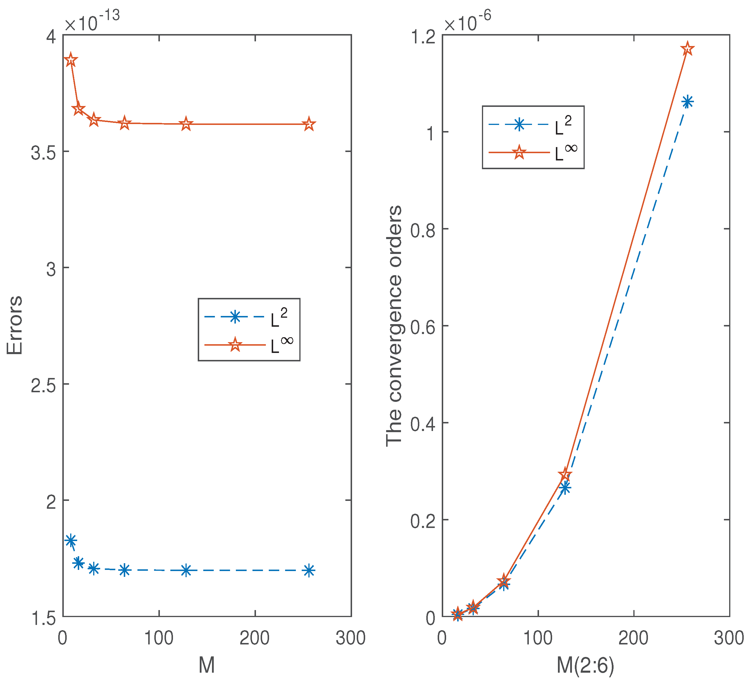Figure 1 shows that the errors $L^{\infty }(M,N)$ and $L^2(M,N)$ calculated by the two algorithms are extremely close, with their magnitudes being only ${10}^{-13}$; the differences in convergence orders are also small, with magnitudes of ${10}^{-6}$.

Setting $M=N$, then $h=\tau$, the error $O(\tau +h^2)=O\left(\tau \right)$. Choosing different $\alpha =0.2,0.4,0.6,0.8$, we use the Crank–Nicolson L1 scheme (13) and the fast Crank–Nicolson L1 scheme (29) to simulate Example 1. The $L^{\infty }(M,N)$, $L^2(M,N)$ errors, the time convergence orders, and CPU time are shown in

Table 2. The $L^{\infty }(M,N)$, $L^2(M,N)$ errors and convergence rates with $M=N$, $\alpha =0.2$ for Example 1.

$\mathit{M}=\mathit{N}$	$\mathbf{CN}-\mathit{L}\mathbf{1}$				$\mathbf{CN}-\mathit{L}\mathbf{1}-\mathbf{SOE}$
	${\mathit{L}}^{\mathbf{2}}$	${\mathit{r}}_{\mathit{\tau }}$	${\mathit{L}}^{\mathbf{\infty }}$	${\mathit{r}}_{\mathit{\tau }}$	${\mathit{L}}^{\mathbf{2}}$	${\mathit{r}}_{\mathit{\tau }}$	${\mathit{L}}^{\mathbf{\infty }}$	${\mathit{r}}_{\mathit{\tau }}$
$2^3$	1.9758 $\times {10}^{-4}$	-	3.8283 $\times {10}^{-4}$	-	1.9758 $\times {10}^{-4}$	-	3.8283 $\times {10}^{-4}$	-
$2^4$	4.9428 $\times {10}^{-5}$	1.9990	9.5467 $\times {10}^{-5}$	2.0036	4.9428 $\times {10}^{-5}$	1.9990	9.5467 $\times {10}^{-5}$	2.0036
$2^5$	1.2360 $\times {10}^{-5}$	1.9997	2.3857 $\times {10}^{-5}$	2.0006	1.2360 $\times {10}^{-5}$	1.9997	2.3857 $\times {10}^{-5}$	2.0006
$2^6$	3.0902 $\times {10}^{-6}$	1.9999	5.9639 $\times {10}^{-6}$	2.0001	3.0902 $\times {10}^{-6}$	1.9999	5.9639 $\times {10}^{-6}$	2.0001
$2^7$	7.7257 $\times {10}^{-7}$	1.9999	1.4910 $\times {10}^{-6}$	2.0000	7.7257 $\times {10}^{-7}$	1.9999	1.4910 $\times {10}^{-6}$	2.0000
$2^8$	1.9316 $\times {10}^{-7}$	1.9999	3.7277 $\times {10}^{-7}$	1.9999	1.9316 $\times {10}^{-7}$	1.9999	3.7277 $\times {10}^{-7}$	1.9999
$2^9$	4.8296 $\times {10}^{-8}$	1.9998	9.3206 $\times {10}^{-8}$	1.9998	4.8296 $\times {10}^{-8}$	1.9998	9.3206 $\times {10}^{-8}$	1.9998
$CPU\left(s\right)$	1040.8125				936.0000

,

Table 3. The $L^{\infty }(M,N)$, $L^2(M,N)$ errors and convergence rates with $M=N$, $\alpha =0.4$ for Example 1.

$\mathit{M}=\mathit{N}$	$\mathbf{CN}-\mathit{L}\mathbf{1}$				$\mathbf{CN}-\mathit{L}\mathbf{1}-\mathbf{SOE}$
	${\mathit{L}}^{\mathbf{2}}$	${\mathit{r}}_{\mathit{\tau }}$	${\mathit{L}}^{\mathbf{\infty }}$	${\mathit{r}}_{\mathit{\tau }}$	${\mathit{L}}^{\mathbf{2}}$	${\mathit{r}}_{\mathit{\tau }}$	${\mathit{L}}^{\mathbf{\infty }}$	${\mathit{r}}_{\mathit{\tau }}$
$2^3$	1.8598 $\times {10}^{-4}$	-	3.5984 $\times {10}^{-4}$	-	1.8598 $\times {10}^{-4}$	-	3.5984 $\times {10}^{-4}$	-
$2^4$	4.6533 $\times {10}^{-5}$	1.9988	8.9758 $\times {10}^{-5}$	2.0033	4.6533 $\times {10}^{-5}$	1.9988	8.9758 $\times {10}^{-5}$	2.0033
$2^5$	1.1635 $\times {10}^{-5}$	1.9998	2.2428 $\times {10}^{-5}$	2.0008	1.1635 $\times {10}^{-5}$	1.9998	2.2428 $\times {10}^{-5}$	2.0008
$2^6$	2.9082 $\times {10}^{-6}$	2.0002	5.6051 $\times {10}^{-6}$	2.0005	2.9082 $\times {10}^{-6}$	2.0002	5.6051 $\times {10}^{-6}$	2.0005
$2^7$	7.2684 $\times {10}^{-7}$	2.0004	1.4008 $\times {10}^{-6}$	2.0005	7.2684 $\times {10}^{-7}$	2.0004	1.4008 $\times {10}^{-6}$	2.0005
$2^8$	1.8164 $\times {10}^{-7}$	2.0006	3.5004 $\times {10}^{-7}$	2.0006	1.8164 $\times {10}^{-7}$	2.0006	3.5004 $\times {10}^{-7}$	2.0006
$2^9$	4.5387 $\times {10}^{-8}$	2.0007	8.7462 $\times {10}^{-8}$	2.0008	4.5387 $\times {10}^{-8}$	2.0007	8.7462 $\times {10}^{-8}$	2.0008
$CPU\left(s\right)$	1214.9844				1002.2813

,

Table 4. The $L^{\infty }(M,N)$, $L^2(M,N)$ errors and convergence rates with $M=N$, $\alpha =0.6$ for Example 1.

$\mathit{M}=\mathit{N}$	$\mathbf{CN}-\mathit{L}\mathbf{1}$				$\mathbf{CN}-\mathit{L}\mathbf{1}-\mathbf{SOE}$
	${\mathit{L}}^{\mathbf{2}}$	${\mathit{r}}_{\mathit{\tau }}$	${\mathit{L}}^{\mathbf{\infty }}$	${\mathit{r}}_{\mathit{\tau }}$	${\mathit{L}}^{\mathbf{2}}$	${\mathit{r}}_{\mathit{\tau }}$	${\mathit{L}}^{\mathbf{\infty }}$	${\mathit{r}}_{\mathit{\tau }}$
$2^3$	1.7455 $\times {10}^{-4}$	-	3.3713 $\times {10}^{-4}$	-	1.7455 $\times {10}^{-4}$	-	3.3713 $\times {10}^{-4}$	-
$2^4$	4.3664 $\times {10}^{-5}$	1.9991	8.4106 $\times {10}^{-5}$	2.0030	4.3664 $\times {10}^{-5}$	1.9991	8.4106 $\times {10}^{-5}$	2.0030
$2^5$	1.0910 $\times {10}^{-5}$	2.0008	2.1001 $\times {10}^{-5}$	2.0018	1.0910 $\times {10}^{-5}$	2.0008	2.1001 $\times {10}^{-5}$	2.0018
$2^6$	2.7242 $\times {10}^{-6}$	2.0018	5.2422 $\times {10}^{-6}$	2.0022	2.7242 $\times {10}^{-6}$	2.0018	5.2422 $\times ‘{10}^{-6}$	2.0022
$2^7$	6.7969 $\times {10}^{-7}$	2.0029	1.3076 $\times {10}^{-6}$	2.0032	6.7969 $\times {10}^{-7}$	2.0029	1.3076 $\times {10}^{-6}$	2.0032
$2^8$	1.6940 $\times {10}^{-7}$	2.0044	3.2580 $\times {10}^{-7}$	2.0049	1.6940 $\times {10}^{-7}$	2.0044	3.2580 $\times {10}^{-7}$	2.0049
$2^9$	4.2153 $\times {10}^{-8}$	2.0067	8.1033 $\times {10}^{-8}$	2.0074	4.2153 $\times {10}^{-8}$	2.0067	8.1033 $\times {10}^{-8}$	2.0074
$CPU\left(s\right)$	1164.5313				1039.2031

and

Table 5. The $L^{\infty }(M,N)$, $L^2(M,N)$ errors and convergence rates with $M=N$,$\alpha =0.8$ for Example 1.

$\mathit{M}=\mathit{N}$	$\mathbf{CN}-\mathit{L}\mathbf{1}$				$\mathbf{CN}-\mathit{L}\mathbf{1}-\mathbf{SOE}$
	${\mathit{L}}^{\mathbf{2}}$	${\mathit{r}}_{\mathit{\tau }}$	${\mathit{L}}^{\mathbf{\infty }}$	${\mathit{r}}_{\mathit{\tau }}$	${\mathit{L}}^{\mathbf{2}}$	${\mathit{r}}_{\mathit{\tau }}$	${\mathit{L}}^{\mathbf{\infty }}$	${\mathit{r}}_{\mathit{\tau }}$
$2^3$	1.6397 $\times {10}^{-4}$	-	3.1619 $\times {10}^{-4}$	-	1.6397 $\times {10}^{-4}$	-	3.1619 $\times {10}^{-4}$	-
$2^4$	4.0996 $\times {10}^{-5}$	1.9999	7.8864 $\times {10}^{-5}$	2.0033	4.0996 $\times {10}^{-5}$	1.9999	7.8864 $\times {10}^{-5}$	2.0033
$2^5$	1.0231 $\times {10}^{-5}$	2.0026	1.9665 $\times {10}^{-5}$	2.0038	1.0231 $\times {10}^{-5}$	2.0026	1.9665 $\times {10}^{-5}$	2.0038
$2^6$	2.5483 $\times {10}^{-6}$	2.0053	4.8955 $\times {10}^{-6}$	2.0061	2.5483 $\times {10}^{-6}$	2.0053	4.8955 $\times {10}^{-6}$	2.0061
$2^7$	6.3286 $\times {10}^{-7}$	2.0096	1.2149 $\times {10}^{-6}$	2.0106	6.3286 $\times {10}^{-7}$	2.0096	1.2149 $\times {10}^{-6}$	2.0106
$2^8$	1.5638 $\times {10}^{-7}$	2.0168	2.9984 $\times {10}^{-7}$	2.0186	1.5638 $\times {10}^{-7}$	2.0168	2.9984 $\times {10}^{-7}$	2.0186
$2^9$	3.8295 $\times {10}^{-8}$	2.0298	7.3265 $\times {10}^{-8}$	2.0330	3.8295 $\times {10}^{-8}$	2.0298	7.3265 $\times {10}^{-8}$	2.0330
$CPU\left(s\right)$	1239.8594				1149.6875

. The data indicate that for different values of $\alpha$, both schemes exhibit the second-order convergence rate, which is higher than the theoretical analysis, and that the time required for the fast Crank–Nicolson L1 scheme (29) is smaller than the Crank–Nicolson L1 scheme (13) computation, but the time difference is not significant due to the small number of time divisions selected. Furthermore, Figure 2 shows that the absolute error between the errors (convergence rates) calculated by the two schemes is very small.

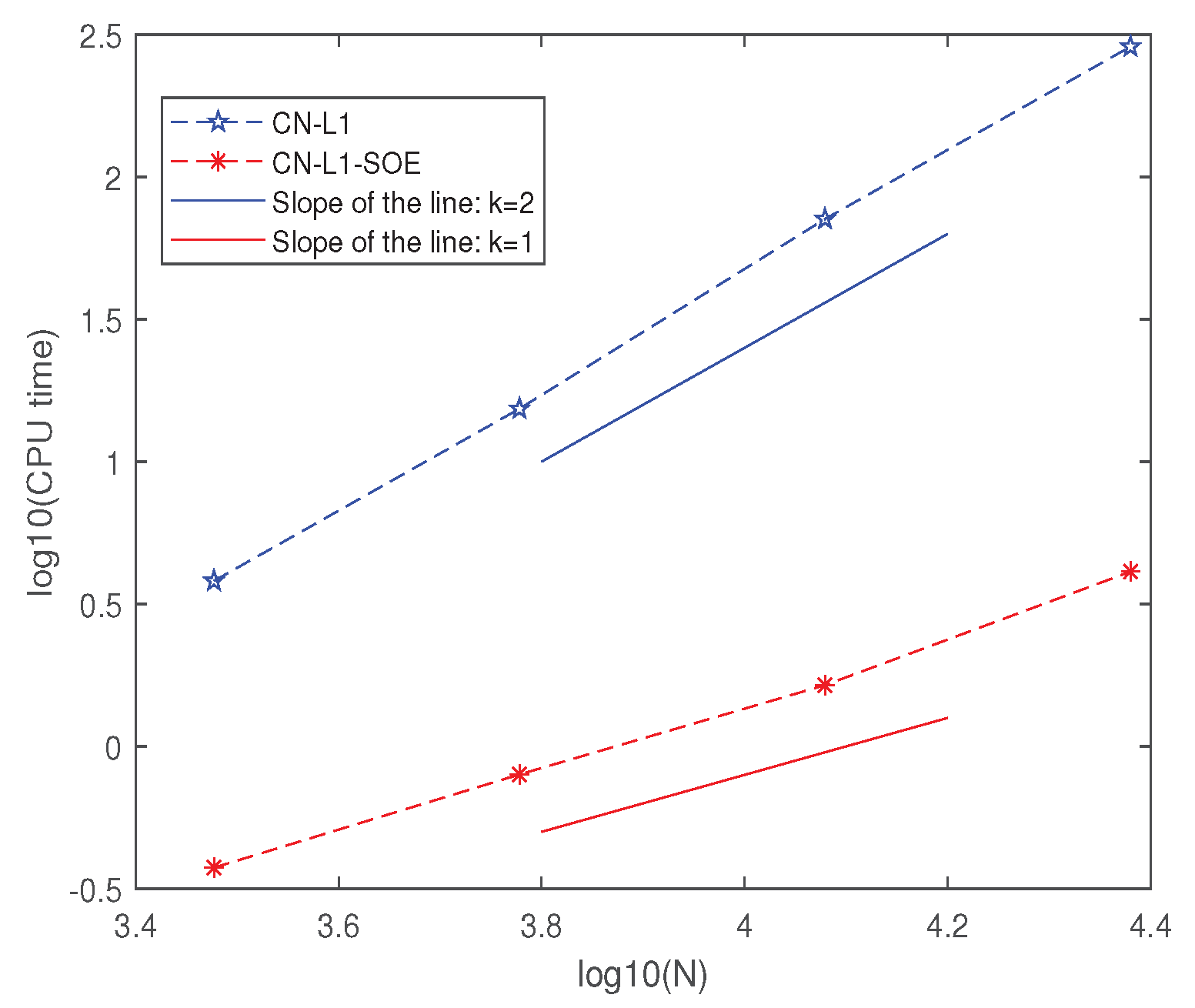
Next, we fix the number of spatial partitions $M=10$ and $\alpha =0.6$ and select larger temporal partitions N. We then use the Crank–Nicolson L1 scheme (13) and the fast Crank–Nicolson L1 scheme (29) to simulate Example 1. The changes in CPU time with respect to the number of temporal partitions are listed in

Table 6. CPU times (in seconds) of Crank–Nicolson L1 scheme (13) and fast Crank–Nicolson L1 scheme (29) with $M=10$, $\alpha =0.6$.

N	3000	6000	12,000	24,000
CN-L1	3.8125	15.3438	71.1406	286.8281
CN-L1-SOE	0.3750	0.7969	1.6406	4.1094

, and an image of CPU time versus temporal partitions is plotted as shown in Figure 3. The data in Table 6 show that when N = 24,000, the Crank–Nicolson L1 scheme (13) takes about 287 s, while the fast Crank–Nicolson L1 scheme (29) only takes over 4 s. In addition, Figure 3 showsthat the CPU time calculated by the Crank–Nicolson L1 scheme is quadratic in the number of partitions N, while the CPU time required by the fast Crank–Nicolson L1 scheme numerical simulation increases linearly with respect to N.

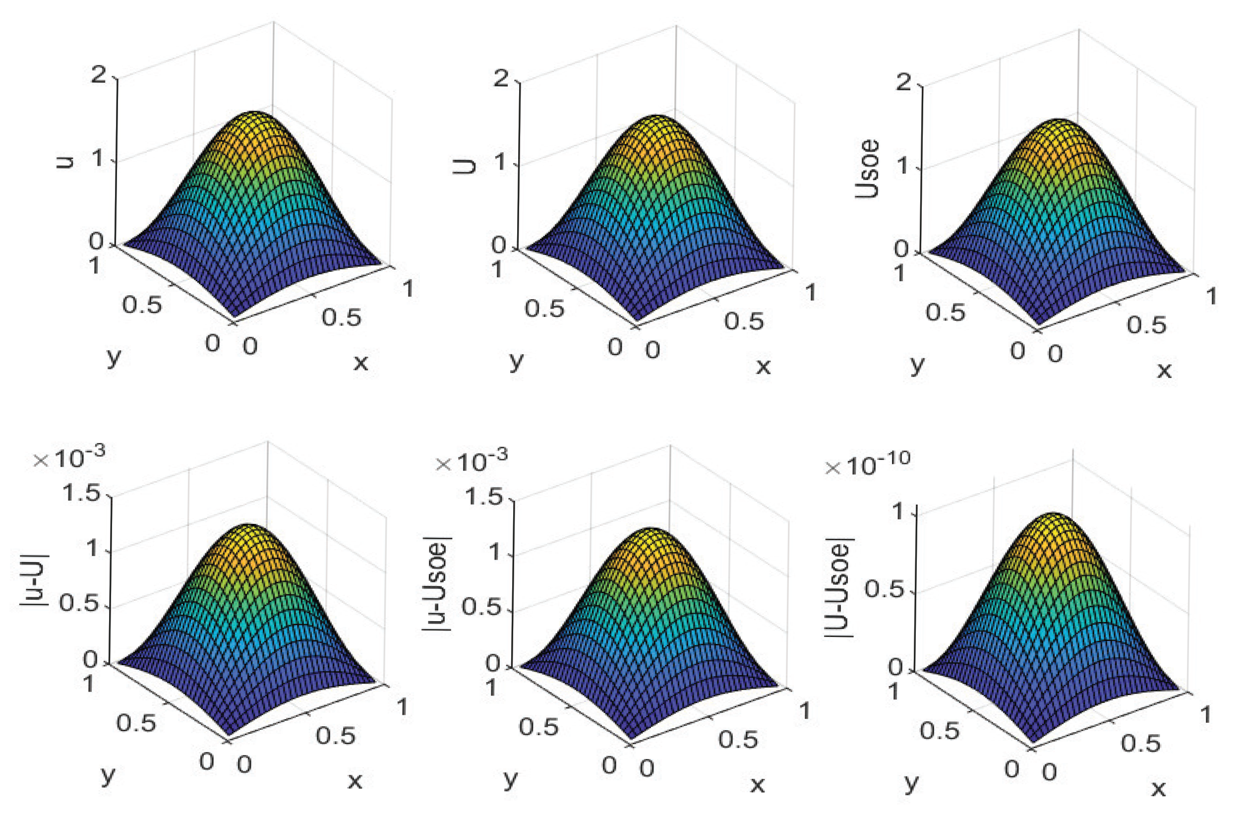
Example 2.

Consider

$$\begin{array}{c}\frac{\partial u}{\partial t}(x,y,t)+{}_0{}^{C}D_t^{\alpha }u(x,y,t)=\frac{{\partial }^{2}u}{\partial x^2}(x,y,t)+\frac{{\partial }^{2}u}{\partial y^2}(x,y,t)+f(x,y,t),(x,y)\in {(0,1)}^2,t\in (0,1],\hfill \\ u(x,y,t)=\varphi (x,y,t),(x,y)\in \partial \Omega ,t\in [0,1],\hfill \\ u(x,y,0)=g(x,y),(x,y)\in \Omega .\hfill \end{array}$$

Assume that the exact solution is $u(x,y,t)=\left[1+\frac{t^{1+\alpha }}{\Gamma (2+\alpha )}\right]sin\pi xsin\pi y$, which satisfies the assumption (3). The corresponding $f(x,y,t)$, $g(x,y)$ and $\varphi (x,y,t)$ can be derived, where

$$f(x,y,t)=\left[\frac{t^{\alpha }}{\Gamma (1+\alpha )}+\frac{t}{\Gamma \left(2\right)}\right]sin\pi xsin\pi y+2{\pi }^{2}sin\pi xsin\pi y\left[1+\frac{t^{1+\alpha }}{\Gamma (2+\alpha )}\right].$$

Setting $M=N=30$, $\alpha =0.6$, the true solution, the numerical solutions computed using the schemes (13) and (29), the absolute errors between the numerical solution and the true solution, and the absolute errors between the two numerical solutions at $t=1$ are plotted in Figure 4. The figure indicates that both numerical solutions approximate the true solution well, and the differences between the two numerical solutions are very small, with magnitudes of ${10}^{-10}$.

Setting $N=5000$, choosing different $\alpha =0.2,0.4,0.6,0.8$ and $M=2^4,2^5,2^6,2^7,2^8$, we solve Example 2 by the fast Crank–Nicolson L1 scheme (29). The computed $L^{\infty }(M,N)$ and $L^2(M,N)$ errors as a function of M are depicted in Figure 5. The figure indicates that for different $\alpha$, as the spatial discretization is refined, the error gradually decreases, with a spatial convergence order of approximately 2.

Setting $M=N$, choosing $\alpha =0.2,0.4,0.6,0.8$, we employ the fast Crank–Nicolson L1 scheme (29) to simulate Example 2, and the computed $L^2(M,N)$ errors and the convergence orders are shown in

Table 7. The $L^2(M,N)$ errors and convergence rates of the scheme (29) with $M=N$ for Example 2.

$\mathit{M}=\mathit{N}$	$\mathit{\alpha }=\mathbf{0.2}$		$\mathit{\alpha }=\mathbf{0.4}$		$\mathit{\alpha }=\mathbf{0.6}$		$\mathit{\alpha }=\mathbf{0.8}$
	${\mathit{L}}^{\mathbf{2}}$	${\mathit{r}}_{\mathit{\tau }}$	${\mathit{L}}^{\mathbf{2}}$	${\mathit{r}}_{\mathit{\tau }}$	${\mathit{L}}^{\mathbf{2}}$	${\mathit{r}}_{\mathit{\tau }}$	${\mathit{L}}^{\mathbf{2}}$	${\mathit{r}}_{\mathit{\tau }}$
$2^3$	1.1205 $\times {10}^{-2}$	-	1.0330 $\times {10}^{-2}$	-	9.4627 $\times {10}^{-3}$	-	8.6820 $\times {10}^{-3}$	-
$2^4$	2.7871 $\times {10}^{-3}$	2.0073	2.5677 $\times {10}^{-3}$	2.0083	2.3463 $\times {10}^{-3}$	2.0119	2.1438 $\times {10}^{-3}$	2.0178
$2^5$	6.9588 $\times {10}^{-4}$	2.0018	6.4047 $\times {10}^{-4}$	2.0033	5.8280 $\times {10}^{-4}$	2.0093	5.2815 $\times {10}^{-4}$	2.0212
$2^6$	1.7392 $\times {10}^{-4}$	2.0004	1.5985 $\times {10}^{-4}$	2.0024	1.4449 $\times {10}^{-4}$	2.0120	1.2887 $\times {10}^{-4}$	2.0351
$2^7$	4.4635 $\times {10}^{-5}$	1.9622	3.9889 $\times {10}^{-5}$	2.0027	3.5676 $\times {10}^{-5}$	2.0179	3.0851 $\times {10}^{-5}$	2.0625
$2^8$	2.2208 $\times {10}^{-5}$	1.0071	9.9491 $\times {10}^{-6}$	2.0033	8.7505 $\times {10}^{-6}$	2.0275	7.1187 $\times {10}^{-6}$	2.1156
$2^9$	1.0790 $\times {10}^{-5}$	1.0414	3.5674 $\times {10}^{-6}$	1.4797	2.1237 $\times {10}^{-6}$	2.0428	1.5211 $\times {10}^{-6}$	2.2265

. The data show that for $\alpha =0.6,0.8$, second-order time convergence is achieved, which exceeds the theoretical convergence order; when $\alpha$ is smaller, as the mesh is refined, the temporal convergence order tends to be first order, consistent with the theoretical analysis. In addition, we used the fully discrete alternating direction implicit (ADI) scheme established in [25] to calculate Example 2. The obtained results are presented in

Table 8. The $L^2(M,N)$ errors and convergence rates of the L1-ADI with $M=N$ for Example 2.

$\mathit{M}=\mathit{N}$	$\mathit{\alpha }=\mathbf{0.2}$		$\mathit{\alpha }=\mathbf{0.4}$		$\mathit{\alpha }=\mathbf{0.6}$		$\mathit{\alpha }=\mathbf{0.8}$
	${\mathit{L}}^{\mathbf{2}}$	${\mathit{r}}_{\mathit{\tau }}$	${\mathit{L}}^{\mathbf{2}}$	${\mathit{r}}_{\mathit{\tau }}$	${\mathit{L}}^{\mathbf{2}}$	${\mathit{r}}_{\mathit{\tau }}$	${\mathit{L}}^{\mathbf{2}}$	${\mathit{r}}_{\mathit{\tau }}$
$2^3$	3.5346 $\times {10}^{-2}$	-	2.7729 $\times {10}^{-2}$	-	1.8927 $\times {10}^{-2}$	-	1.0410 $\times {10}^{-2}$	-
$2^4$	1.1495 $\times {10}^{-2}$	1.6205	9.3443 $\times {10}^{-3}$	1.5692	6.3885 $\times {10}^{-3}$	1.5669	3.2066 $\times {10}^{-3}$	1.6989
$2^5$	3.2516 $\times {10}^{-3}$	1.8219	2.7202 $\times {10}^{-3}$	1.7804	1.8558 $\times {10}^{-3}$	1.7834	7.9451 $\times {10}^{-4}$	2.0129
$2^6$	8.5323 $\times {10}^{-4}$	1.9301	7.1979 $\times {10}^{-4}$	1.9181	4.7806 $\times {10}^{-4}$	1.9568	3.1457 $\times {10}^{-4}$	1.3367
$2^7$	2.9564 $\times {10}^{-4}$	1.5291	2.5030 $\times {10}^{-4}$	1.5239	1.7607 $\times {10}^{-4}$	1.4410	1.4818 $\times {10}^{-4}$	1.0860
$2^8$	1.7540 $\times {10}^{-4}$	0.7532	1.3547 $\times {10}^{-4}$	0.8857	8.8698 $\times {10}^{-5}$	0.9892	7.1268 $\times {10}^{-5}$	1.0561
$2^9$	9.8947 $\times {10}^{-5}$	0.8259	7.1485 $\times {10}^{-5}$	0.9222	4.4494 $\times {10}^{-5}$	0.9953	3.4639 $\times {10}^{-5}$	1.0408

. By comparing with the data in Table 7, it can be observed that the algorithm constructed in this paper yields more accurate computation results.

Next, the algorithm established in this paper calculates Example 2 on time-graded meshes. The time node set is given by ${\Omega }_{\tau }=\left\{t_n\right|t_n=T{\left(\frac{n}{N}\right)}^r,n=0,1,2,\cdots ,N\}$, where r is the parameter of the graded meshes. We set $M=N$ and $\alpha =0.6$, selecting different values for r. The results are presented in

Table 9. The $L^2(M,N)$ errors and convergence rates of the scheme (29) on graded meshes with $M=N$, $\alpha =0.6$ for Example 2.

$\mathit{M}=\mathit{N}$	$\mathit{r}=\mathbf{2}$		$\mathit{r}=\mathbf{4}$		$\mathit{r}=\mathbf{6}$		$\mathit{r}=\mathbf{8}$
	${\mathit{L}}^{\mathbf{2}}$	${\mathit{r}}_{\mathit{\tau }}$	${\mathit{L}}^{\mathbf{2}}$	${\mathit{r}}_{\mathit{\tau }}$	${\mathit{L}}^{\mathbf{2}}$	${\mathit{r}}_{\mathit{\tau }}$	${\mathit{L}}^{\mathbf{2}}$	${\mathit{r}}_{\mathit{\tau }}$
$2^3$	7.5493 $\times {10}^{-3}$	-	4.9609 $\times {10}^{-3}$	-	9.8903 $\times {10}^{-3}$	-	2.2025 $\times {10}^{-2}$	-
$2^4$	1.8584 $\times {10}^{-3}$	2.0223	1.1735 $\times {10}^{-3}$	2.0798	2.9136 $\times {10}^{-3}$	1.7632	6.7808 $\times {10}^{-3}$	1.6996
$2^5$	4.5629 $\times {10}^{-4}$	2.0260	2.8529 $\times {10}^{-4}$	2.0403	7.8943 $\times {10}^{-4}$	1.8839	1.8362 $\times {10}^{-3}$	1.8847
$2^6$	1.1111 $\times {10}^{-4}$	2.0380	6.9415 $\times {10}^{-5}$	2.0391	2.1274 $\times {10}^{-4}$	1.8917	4.8571 $\times {10}^{-4}$	1.9186
$2^7$	2.6672 $\times {10}^{-5}$	2.0586	1.6752 $\times {10}^{-5}$	2.0509	5.8385 $\times {10}^{-5}$	1.8654	1.2949 $\times {10}^{-4}$	1.9072
$2^8$	6.2511 $\times {10}^{-6}$	2.0932	3.9849 $\times {10}^{-6}$	2.0717	1.6501 $\times {10}^{-5}$	1.8231	3.5246 $\times {10}^{-5}$	1.8774
$2^9$	1.4051 $\times {10}^{-6}$	2.1534	1.0640 $\times {10}^{-6}$	1.9051	4.8379 $\times {10}^{-6}$	1.7701	9.8781 $\times {10}^{-6}$	1.8351

. Comparing with the results in Table 7 for $\alpha =0.6$, we find that due to the weak singularity of the solution at the initial moment, selecting an appropriate parameter, such as $r=2$ or 4, leads to time nodes that are suitably close to $t=0$, resulting in more accurate calculations compared to those obtained on uniform meshes. However, when the value of r is too large, the distribution of time nodes becomes severely uneven, leading to increased errors.

6. Conclusions

In this paper, we establish a Crank–Nicolson L1 scheme on uniform meshes for the two-dimensional time fractional mobile/immobile equation with weak singularity at the initial moment. The error is estimated using the energy analysis method. The obtained error estimate has a convergence order of $O(h^2+\tau )$, but the numerical simulation calculations yield a spatial convergence order of 2, and the temporal convergence order is superior to the first order as theoretically analyzed.

Furthermore, considering the historical dependence of the time fractional derivative, the numerical simulation of the Crank–Nicolson L1 scheme requires a large amount of memory and expensive computation; we adopted the sum-of-exponentials approximation technology to discretize the fractional derivative and established a fast Crank–Nicolson L1 scheme. Through numerical simulation, it can be found that when the number of time steps N is large, the efficiency of the fast algorithm is significantly higher than the Crank–Nicolson L1 scheme. In addition, the difference between the calculated results of the fast Crank–Nicolson L1 scheme (29) and the Crank–Nicolson L1 scheme (13) is particularly small, but there is no strict error estimate for the fast Crank–Nicolson L1 scheme (29), which we will study in the future. The algorithm proposed in this paper is also applicable to other fractional models and provides a technical foundation for solving the practical problems described by model (1).

The time fractional mobile/immobile models have wide applications in various fields, such as modeling groundwater solute transport, describing thermal diffusion, and ocean sound propagation. Conducting effective numerical algorithm research on these models can promote the solution of practical problems. This paper has systematically investigated the two-dimensional time fractional mobile/immobile model. However, considering that the three-dimensional model is closer to the actual situation, we will further consider extending algorithms to three-dimensional models based on this research.