Stat-Space Approach to Three-Dimensional Thermoelastic Half-Space Based on Fractional Order Heat Conduction and Variable Thermal Conductivity Under Moor–Gibson–Thompson Theorem

Abstract

This study presents a mathematical model of a three-dimensional thermoelastic half-space with variable thermal conductivity under the definition of fractional order heat conduction based on the Moor–Gibson–Thompson theorem. The non-dimensional governing equations using Laplace and double Fourier transform methods have been applied to a three-dimensional thermoelastic, isotropic, and homogeneous half-space exposed to a rectangular thermal loading pulse with a traction-free surface. The double Fourier transforms and Laplace transform inversions have been computed numerically. The numerical distributions of temperature increment, invariant stress, and invariant strain have been shown and analysed. The fractional order parameter and the variability of thermal conductivity significantly influence all examined functions and the behaviours of the thermomechanical waves. Classifying thermal conductivity as weak, normal, and strong is crucial and closely corresponds to the actual behaviour of the thermal conductivity of thermoelastic materials.

1. Introduction

There are two predictions made by uncoupled thermoelasticity that go against how thermoelastic materials behave. Although elastic changes cause heat changes, the type of the heat conduction equation is parabolic in form and independent from the elastic effect; this makes the thermal waves propagate at unlimited speed. The uncoupled theory of thermoelasticity has a flaw that Biot sought to address by proposing coupled thermoelasticity (CTE) [1,2,3]. Consistent with actual behaviour, hyperbolic motion equations of coupled thermoelasticity and diffusion-type heat conduction equations provide limitless speeds of thermal changes. Lord and Shulman presented several changes to dynamic thermoelasticity models to resolve the second conundrum [4,5,6,7], while Green and Lindsay [3,8,9,10] and Green and Naghdi [11,12,13,14] depended on the definition of the second sound phenomenon. Many applications in the context of the above theories have been constructed and solved [15,16,17,18,19] and some other problems have been solved in [20,21,22,23]. The Moore–Gibson–Thompson (MGT) equation arises from fluid mechanics and has obtained high levels of interest in recent years, with many papers being directed to studying and understanding it [24,25,26,27,28] and some other applications in [29,30,31]. State-space approaches, a crucial component of modern control theory, underpin several studies on stochastic systems, optimal control, and nonlinear systems. This approach can solve any quantity of independent first-order differential equations; hence, the order is not a limitation [32,33]. This technique is advantageous as it facilitates the rapid development of computer programs to address problems and analyse linear time-invariant systems. Bahar and Hetnarski have developed a technique for addressing thermoelastic issues using state-space variables, including temperature increase, displacement, strain, and their gradients. This approach entails reformulating the governing equations of the problem inside this framework [34]. The fractional order calculus is often used in a more generalized sense, including various transport phenomena [35]. Youssef presented a novel formula for heat conduction derived from the Riemann–Liouville fractional integral, which serves as an extension of the established n-fold repeating integral $\left(I^{n}f\left(t\right)\right)$ [36,37,38]. Many applications have been solved in the context of the Youssef model of fractional order heat conduction [19,37,39,40,41]. Godfrey found that different samples of silicon nitride had thermal conductivities that dropped by as much as 45% between 1 and 400 degrees Celsius. Therefore, it is crucial to understand how these changes impact the distributions of stress and displacement in metal components [42]. Therefore, it is crucial to consider the temperature dependency of material characteristics while doing the thermal stress analysis. With the assumption of variable thermal conductivity, several applications have been developed and addressed [18,43,44]. Mirparizi and Razavinasab present a modified Green–Lindsay (MGL) thermoelasticity model considering temperature and strain rate [45]. Mirparizi et al. solved one-dimensional electro-magneto-poro-thermoelastic wave propagation in a functionally graded medium with energy dissipation in the context of the modified Green–Lindsay theorem (MGL) [46]. Mirparizi et al. studied the large deformation Hermitian finite element coupled thermoelasticity analysis of wave propagation and reflection in a finite domain [47].

Thus, this paper aims to present a mathematical model of a three-dimensional space that can expand and contract due to heat, considering changes in thermal conductivity. The novelty of this model is based on a specific heat transfer theory related to the Moor–Gibson–Thompson theorem. The main equations, which do not have specific measurements, were used with Laplace and double Fourier transforms on a three-dimensional material that is uniform and has the same properties in all directions. This material is a half-space that experiences a rectangular pulse of heat while its surface is free from any pressure. The double Fourier transforms and the inversions of the Laplace transforms have been calculated by using numerical methods.

2. The Governing Equations

The governing equation of a homogeneous, isotropic, and elastic material within the framework of generalized thermoelasticity, including fractional order heat conduction and a single relaxation period, devoid of heat sources or external body forces in general coordinates, is expressed as follows:

The equations of motion are as follows [16,48]:

$$\mu u_{i,jj}+\left(\lambda +\mu \right)u_{j,ij}-\gamma {\theta }_{,i}=\rho {\ddot{u}}_i,i,j=x,y,z$$

(1)

where $u_i$ gives the components of the displacement vector, $\theta =\left(T-T_0\right)$ is the temperature increment, $T_o$ is the reference temperature, $\rho$ is the density, $\lambda , \mu$ are Lame’s constants (elastic parameters), $\gamma ={\alpha }_T\left(3\lambda +2\mu \right)$ in which ${\alpha }_T$ is the coefficient of linear thermal expansion, and $i,j=x,y,z$ refer to the Cartesian coordinates.

The heat conduction equation for a homogeneous, isotropic, and elastic material under Moor–Gibson–Thompson (MGT) in the usual form is as follows [24,25]:

$${\left(K\left(\theta \right){\dot{\theta }}_{,i}+K^{*}\left(\theta \right){\theta }_{,i}\right)}_{,i}=\left(1+{\tau }_q{\displaystyle \frac{\partial }{\partial t}}\right)\left({\displaystyle \frac{\partial }{\partial t}}\left(\rho C_E\dot{\theta }\right)+T_0\gamma \ddot{e}\right), i=x,y,z$$

(2)

where $K\left(\theta \right)$ and $K^{*}\left(\theta \right)$ are the thermal conductivity and the thermal conductivity rate, respectively, $C_E$ gives the specific heat at constant strain, and $e$ is the sum of the principal strains which gives the cubical dilatation.

The following relation will be considered:

$$K\left(\theta \right)\approx {\tau }_K{K}^{*}\left(\theta \right)$$

(3)

where ${\tau }_K>0$ gives the lag time of the temperature gradient. Then, we have the classical heat conduction equation based on the Moor–Gibson–Thompson theorem as follows:

$${\left[K^{*}\left(\theta \right)\left({\tau }_K{\dot{\theta }}_{,i}+{\theta }_{,i}\right)\right]}_{,i}=\left(1+{\tau }_q{\displaystyle \frac{\partial }{\partial t}}\right)\left({\displaystyle \frac{\partial }{\partial t}}\left(\rho C_E\dot{\theta }\right)+T_0\gamma \ddot{e}\right)$$

(4)

Moreover, the following relation is satisfied [32]:

$$\rho C_E={\displaystyle \frac{K\left(\theta \right)}{\kappa }}={\displaystyle \frac{{\tau }_K{K}^{*}\left(\theta \right)}{\kappa }}$$

(5)

where $\kappa$ is the diffusivity of the material.

According to Youssef’s model of the fractional order heat conduction equation, we have [38]:

$${\left[I^{\upsilon -1}{K}^{*}\left(\theta \right)\left({\tau }_K{\dot{\theta }}_{,i}+{\theta }_{,i}\right)\right]}_{,i}=\left(1+{\tau }_q{\displaystyle \frac{\partial }{\partial t}}\right)\left({\displaystyle \frac{{\tau }_K}{\kappa }}{\displaystyle \frac{\partial }{\partial t}}\left(K^{*}\left(\theta \right)\dot{\theta }\right)+T_0\gamma \ddot{e}\right)$$

(6)

where $I^{\alpha }$ defines the Riemann–Liouville fractional integral written in a convolution-type form as in [24,25,26]:

$$I_t^{\upsilon }f\left(t\right)=\left\{\begin{array}{cc}{\displaystyle \frac{1}{\mathrm{\Gamma }\left(\upsilon \right)}}{\displaystyle \underset{0}{\overset{t}{\int }}{\left(t-\tau \right)}^{\upsilon -1}f\left(\tau \right)}d\tau & 0<\upsilon \le 2\\ f\left(t\right)& \upsilon =0\end{array}\right\}$$

(7)

Moreover,

$$\left\{\begin{array}{cc}0<\upsilon <1& \mathrm{gives}\mathrm{weak}\mathrm{condutivity}\\ \upsilon =1& \mathrm{gives}\mathrm{normal}\mathrm{condutivity}\\ 1<\upsilon \le 2& \mathrm{gives}\mathrm{strong}\mathrm{condutivity}\end{array}\right\}$$

(8)

The constitutive relations are in the form:

$${\sigma }_{ij}=2\mu e_{ij}+\left(\lambda e_{kk}-\gamma \theta \right){\delta }_{ij}, i,j=x,y,z$$

(9)

The strain–displacement relations have the following forms:

$$2e_{ij}=u_{i,j}+u_{j,i}, i,j=x,y,z$$

(10)

We will use the following equation [18,48]:

$$\vartheta ={\displaystyle \frac{1}{K_o}}{\displaystyle \underset{0\hspace{1em}}{\overset{\theta }{\int }}{K}^{*}\left(\zeta \right) d\zeta }$$

(11)

where $K_o$ is the thermal conductivity rate at room temperature and it is constant.

By differentiating Equation (11) to the coordinates $x_i$, we obtain:

$$K_o{\vartheta }_{,i}=K^{*}\left(\theta \right){\theta }_{,i}$$

(12)

By differentiating to the coordinates $x_i$, we have:

$$K_o {\vartheta }_{,ii}={\left[K^{*}\left(\theta \right){\theta }_{,i}\right]}_{,i}$$

(13)

By differentiating Equation (11) to time, we obtain:

$$K^{*}\left(\theta \right) \dot{\theta }=K_o \dot{\vartheta } \mathrm{and} {\displaystyle \frac{\partial }{\partial t}}\left[K^{*}\left(\theta \right) \dot{\theta }\right]=K_o \ddot{\vartheta }$$

(14)

Hence, we obtain:

$$I^{\upsilon -1}{K}_o\left({\tau }_K{\dot{\vartheta }}_{,ii}+{\vartheta }_{,ii}\right)=\left(1+{\tau }_q{\displaystyle \frac{\partial }{\partial t}}\right)\left({\displaystyle \frac{{\tau }_K{K}_o}{\kappa }}\ddot{\vartheta }+T_0\gamma \ddot{e}\right)$$

(15)

We approximate the variation of the thermal diffusivity with temperature by the following linear law:

$$K^{*}\left(\theta \right)=K_o\left(1+K_1\theta \right)$$

(16)

$K_1$ is a minor constant that may assume positive or negative values depending on the material qualities, since the thermal conductivity of some materials rises, while it decreases for others, with heating.

By substituting Equation (16) into the mapping in Equation (11), we obtain:

$$\vartheta =\theta +{\displaystyle \frac{K_1}{2}}{\theta }^2$$

(17)

which gives:

$${\vartheta }_{,i}={\theta }_{,i}+K_1\theta {\theta }_{,i}$$

(18)

Substituting this in Equation (1), we obtain:

$$\left(\lambda +\mu \right)u_{j,ij}+\mu u_{i,jj}-\gamma {\vartheta }_{,i}+\gamma K_1\theta {\theta }_{,i}=\rho {\ddot{u}}_i$$

(19)

and

$${\sigma }_{ij}=2\mu e_{ij}+\lambda e_{kk}{\delta }_{ij}+\left({\displaystyle \frac{K_1}{2}}{\theta }^2-\vartheta \right)\gamma {\delta }_{ij}$$

(20)

For linearization, we will neglect the small nonlinear terms. Hence, we obtain:

$$\left(\lambda +\mu \right)u_{j,ij}+\mu u_{i,jj}-\gamma {\vartheta }_{,i}=\rho {\ddot{u}}_i$$

(21)

and

$${\sigma }_{ij}=2\mu e_{ij}+\lambda e_{kk}{\delta }_{ij}-\gamma \vartheta {\delta }_{ij}$$

(22)

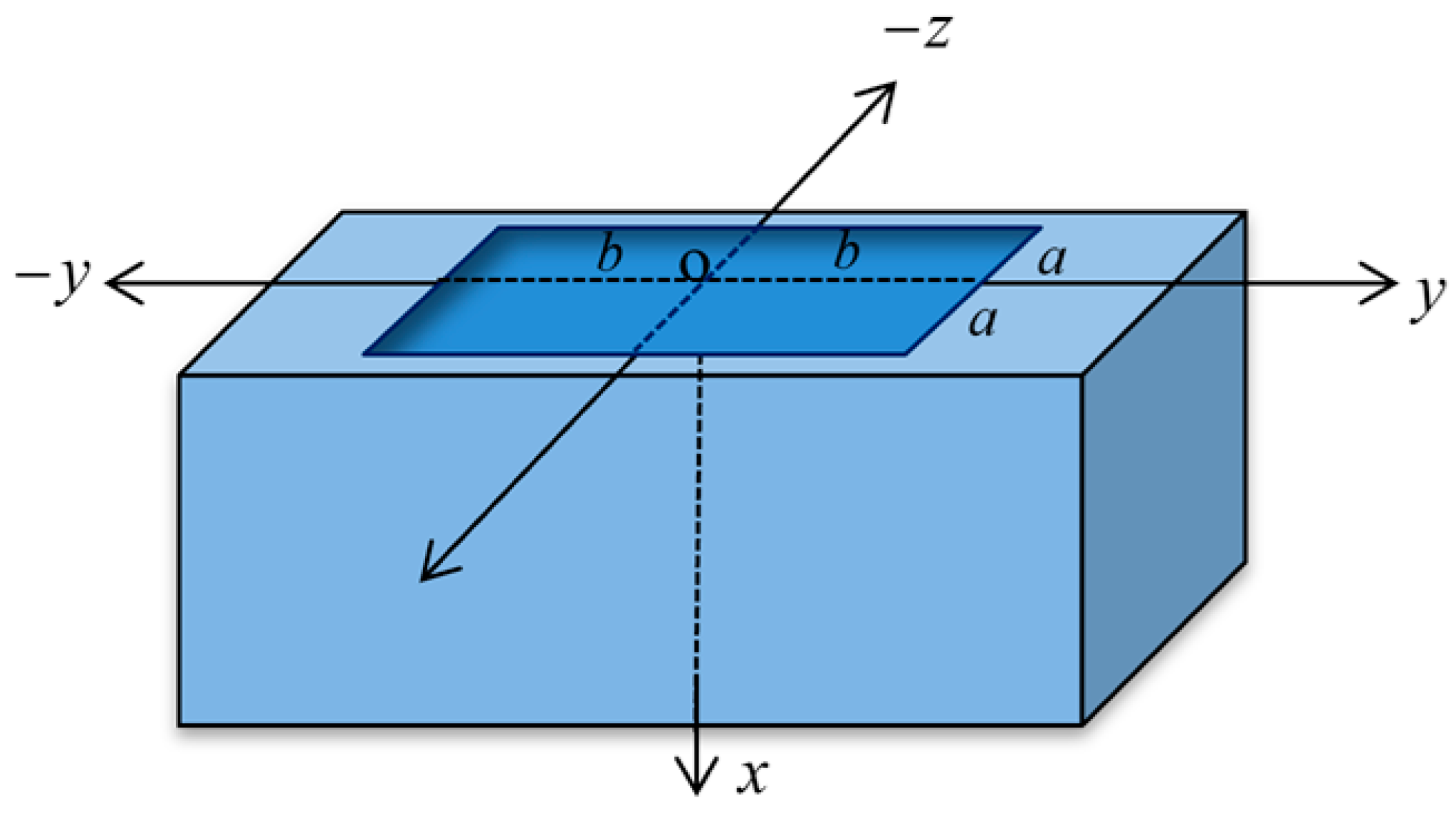
3. The Problem Formulation

Consider that a homogeneous, isotropic, thermoelastic, and three-dimensional material occupies the region $\mathsf{\Omega }$, which is defined by:

$$\mathsf{\Omega }=\left\{x,y,z:0\le x<\infty ,-\infty <y<\infty ,-\infty <z<\infty \right\}$$

(23)

We assume the material has no external forces, has no heat sources, is initially quiescent, and has been shocked thermally when traction-free on the bounding surface $x=0$ as in Figure 1.

By using the Cartesian coordinates $\left(x,y,z\right)$, the components of the displacement are as follows:

$$\left(u_x,u_y,u_z\right)=\left(u,v,w\right)$$

(24)

The equations of motion have the following formulas:

$$\rho \ddot{u}=\left(\lambda +2\mu \right){\displaystyle \frac{{\partial }^{2}u}{\partial x^2}}+\left(\lambda +\mu \right)\left({\displaystyle \frac{{\partial }^{2}v}{\partial x\partial y}}+{\displaystyle \frac{{\partial }^{2}w}{\partial x\partial z}}\right)+\mu \left({\displaystyle \frac{{\partial }^{2}u}{\partial y^2}}+{\displaystyle \frac{{\partial }^{2}u}{\partial z^2}}\right)-\gamma {\displaystyle \frac{\partial \vartheta }{\partial x}}$$

(25)

$$\rho \ddot{v}=\left(\lambda +2\mu \right){\displaystyle \frac{{\partial }^{2}v}{\partial y^2}}+\left(\lambda +\mu \right)\left({\displaystyle \frac{{\partial }^{2}u}{\partial x\partial y}}+{\displaystyle \frac{{\partial }^{2}w}{\partial z\partial y}}\right)+\mu \left({\displaystyle \frac{{\partial }^{2}v}{\partial x^2}}+{\displaystyle \frac{{\partial }^{2}v}{\partial z^2}}\right)-\gamma {\displaystyle \frac{\partial \vartheta }{\partial y}}$$

(26)

and

$$\rho \ddot{w}=\left(\lambda +2\mu \right){\displaystyle \frac{{\partial }^{2}w}{\partial z^2}}+\left(\lambda +\mu \right)\left({\displaystyle \frac{{\partial }^{2}u}{\partial z\partial x}}+{\displaystyle \frac{{\partial }^{2}v}{\partial z\partial y}}\right)+\mu \left({\displaystyle \frac{{\partial }^{2}w}{\partial x^2}}+{\displaystyle \frac{{\partial }^{2}w}{\partial y^2}}\right)-\gamma {\displaystyle \frac{\partial \vartheta }{\partial z}}$$

(27)

The heat conduction equation has the following form:

$$I^{\upsilon -1}{K}_o\left(1+{\tau }_K{\displaystyle \frac{\partial }{\partial t}}\right)\left({\displaystyle \frac{{\partial }^2\vartheta }{\partial x^2}}+{\displaystyle \frac{{\partial }^2\vartheta }{\partial y^2}}+{\displaystyle \frac{{\partial }^2\vartheta }{\partial z^2}}\right)=\left(1+{\tau }_q{\displaystyle \frac{\partial }{\partial t}}\right)\left({\displaystyle \frac{{\tau }_K{K}_o}{\kappa }}\ddot{\vartheta }+T_0\gamma \ddot{e}\right)$$

(28)

The constitutive relations are in the forms:

$${\sigma }_{xx}=2\mu e_{xx}+\lambda e-\gamma \vartheta$$

(29)

$${\sigma }_{yy}=2\mu e_{yy}+\lambda e-\gamma \vartheta$$

(30)

$${\sigma }_{zz}=2\mu e_{zz}+\lambda e-\gamma \vartheta$$

(31)

and

$${\sigma }_{xy}=2\mu e_{xy}, {\sigma }_{xz}=2\mu e_{xz}, {\sigma }_{yz}=2\mu e_{yz}$$

(32)

The strain–displacement relations have the following forms:

$$e_{xx}={\displaystyle \frac{\partial u}{\partial x}}, e_{yy}={\displaystyle \frac{\partial v}{\partial y}}, e_{zz}={\displaystyle \frac{\partial w}{\partial z}},$$

(33)

$$e_{xy}={\displaystyle \frac{1}{2}}\left({\displaystyle \frac{\partial u}{\partial y}}+{\displaystyle \frac{\partial v}{\partial x}}\right), e_{xz}={\displaystyle \frac{1}{2}}\left({\displaystyle \frac{\partial u}{\partial z}}+{\displaystyle \frac{\partial w}{\partial x}}\right), e_{yz}={\displaystyle \frac{1}{2}}\left({\displaystyle \frac{\partial w}{\partial y}}+{\displaystyle \frac{\partial v}{\partial z}}\right)$$

(34)

and

$$e={\displaystyle \frac{\partial u}{\partial x}}+{\displaystyle \frac{\partial v}{\partial y}}+{\displaystyle \frac{\partial w}{\partial z}}=e_{xx}+e_{yy}+e_{zz}$$

(35)

We can re-write Equations (25)–(27) by using Equation (35) to give the following forms:

$$\rho {\displaystyle \frac{\partial \ddot{u}}{\partial x}}=\left(\lambda +\mu \right){\displaystyle \frac{{\partial }^{2}e}{\partial x^2}}+\mu {\nabla }^2{\displaystyle \frac{\partial u}{\partial x}}-\gamma {\displaystyle \frac{{\partial }^2\vartheta }{\partial x^2}}$$

(36)

$$\rho {\displaystyle \frac{\partial \ddot{v}}{\partial y}}=\left(\lambda +\mu \right){\displaystyle \frac{{\partial }^{2}e}{\partial y^2}}+\mu {\nabla }^2{\displaystyle \frac{\partial v}{\partial y}}-\gamma {\displaystyle \frac{{\partial }^2\vartheta }{\partial y^2}}$$

(37)

and

$$\rho {\displaystyle \frac{\partial \ddot{w}}{\partial z}}=\left(\lambda +\mu \right){\displaystyle \frac{{\partial }^{2}e}{\partial z^2}}+\mu {\nabla }^2{\displaystyle \frac{\partial w}{\partial z}}-\gamma {\displaystyle \frac{{\partial }^2\vartheta }{\partial z^2}}$$

(38)

where ${\nabla }^2={\displaystyle \frac{{\partial }^2}{\partial x^2}}+{\displaystyle \frac{{\partial }^2}{\partial y^2}}+{\displaystyle \frac{{\partial }^2}{\partial z^2}}$.

The heat conduction equation takes the form:

$$I^{\upsilon -1}\left(1+{\tau }_K{\displaystyle \frac{\partial }{\partial t}}\right){\nabla }^2\vartheta =\left({\displaystyle \frac{{\partial }^2}{\partial t^2}}+{\tau }_q{\displaystyle \frac{{\partial }^3}{\partial t^3}}\right)\left({\displaystyle \frac{{\tau }_K}{\kappa }}\vartheta +{\displaystyle \frac{T_0\gamma }{K_o}}e\right)$$

(39)

Now, the following dimensionless variables will be used [16]:

$\left(x^{\prime },y^{\prime },z^{\prime }\right)=c\eta \left(x,y,z\right)$, $\left(t^{\prime },{{\tau }^{\prime }}_K,{{\tau }^{\prime }}_q\right)=c^2\eta \left(t,{\tau }_K,{\tau }_q\right)$, $\left({\vartheta }^{\prime },\theta \right)={\displaystyle \frac{\gamma }{\lambda +2\mu }}\left(\vartheta ,\theta \right)$, ${{\sigma }^{\prime }}_{ij}={\displaystyle \frac{{\sigma }_{ij}}{\lambda +2\mu }}$, $c=\sqrt{{\displaystyle \frac{\lambda +2\mu }{\rho }}}$, $\eta ={\displaystyle \frac{1}{\kappa }}$.

Thus, we obtain:

$${\displaystyle \frac{\partial \ddot{u}}{\partial x}}=\left(1-\beta \right){\displaystyle \frac{{\partial }^{2}e}{\partial x^2}}+\beta {\nabla }^2{\displaystyle \frac{\partial u}{\partial x}}-{\displaystyle \frac{{\partial }^2\vartheta }{\partial x^2}}$$

(40)

$${\displaystyle \frac{\partial \ddot{v}}{\partial y}}=\left(1-\beta \right){\displaystyle \frac{{\partial }^{2}e}{\partial y^2}}+\beta {\nabla }^2{\displaystyle \frac{\partial v}{\partial y}}-{\displaystyle \frac{{\partial }^2\vartheta }{\partial y^2}}$$

(41)

$${\displaystyle \frac{\partial \ddot{w}}{\partial z}}=\left(1-\beta \right){\displaystyle \frac{{\partial }^{2}e}{\partial z^2}}+\beta {\nabla }^2{\displaystyle \frac{\partial w}{\partial z}}-{\displaystyle \frac{{\partial }^2\vartheta }{\partial z^2}}$$

(42)

$$I^{\upsilon -1}\left(1+{\tau }_K{\displaystyle \frac{\partial }{\partial t}}\right){\nabla }^2\vartheta =\left({\displaystyle \frac{{\partial }^2}{\partial t^2}}+{\tau }_q{\displaystyle \frac{{\partial }^3}{\partial t^3}}\right)\left({\epsilon }_{\upsilon }\vartheta +{\epsilon }_{1}e\right)$$

(43)

$${\sigma }_{xx}=2\beta e_{xx}+\left(1-2\beta \right)e-\vartheta$$

(44)

$${\sigma }_{yy}=2\beta e_{yy}+\left(1-2\beta \right)e-\vartheta$$

(45)

$${\sigma }_{zz}=2\beta e_{zz}+\left(1-2\beta \right)e-\vartheta$$

(46)

and

$${\sigma }_{xy}=2\beta e_{xy}, {\sigma }_{xz}=\beta e_{xz}, {\sigma }_{yz}=2\beta e_{yz}$$

(47)

where $\beta ={\displaystyle \frac{\mu }{\lambda +2\mu }}$, ${\epsilon }_{\upsilon }={\tau }_K{\left(c^2\eta \right)}^{\upsilon -1}$, and ${\epsilon }_1={\displaystyle \frac{{\left(c^2\eta \right)}^{\upsilon }{\gamma }^2{T}_0}{\left(\lambda +2\mu \right)\eta K_o}}$.

For simplicity, the primes have been dropped.

By summing Equations (40)–(42) and using Equation (35), we obtain:

$$\ddot{e}={\nabla }^{2}e-{\nabla }^2\vartheta$$

(48)

The invariant stress $\sigma$ is the average value of the principal stresses as follows:

$$\sigma ={\displaystyle \frac{1}{3}}\left({\sigma }_{xx}+{\sigma }_{yy}+{\sigma }_{yy}\right)$$

(49)

By using Equations (44)–(46), we obtain:

$$\sigma =\alpha e-\vartheta$$

(50)

where $\alpha =1-{\displaystyle \frac{4}{3}}\beta$.

4. Applying the Laplace and Double Fourier Transforms

By using the Laplace transform defined for any function $g\left(x,y,z,t\right)$, we obtain the following equation:

$$\overline{g}\left(x,y,z,s\right)={\displaystyle \underset{0}{\overset{\infty }{\int }}g\left(x,y,z,t\right) e^{-st} dt}$$

(51)

Then, we obtain:

$$s^2{\overline{e}}_{xx}=\left(1-\beta \right){\displaystyle \frac{{\partial }^2\overline{e}}{\partial x^2}}+\beta {\nabla }^2{\displaystyle \frac{\partial \overline{u}}{\partial x}}-{\displaystyle \frac{{\partial }^2\overline{\vartheta }}{\partial x^2}}$$

(52)

$$s^2{\overline{e}}_{yy}=\left(1-\beta \right){\displaystyle \frac{{\partial }^2\overline{e}}{\partial y^2}}+\beta {\nabla }^2{\displaystyle \frac{\partial \overline{v}}{\partial y}}-{\displaystyle \frac{{\partial }^2\overline{\vartheta }}{\partial y^2}}$$

(53)

$$s^2{\overline{e}}_{zz}=\left(1-\beta \right){\displaystyle \frac{{\partial }^2\overline{e}}{\partial z^2}}+\beta {\nabla }^2{\displaystyle \frac{\partial \overline{w}}{\partial z}}-{\displaystyle \frac{{\partial }^2\overline{\vartheta }}{\partial z^2}}$$

(54)

$$\left({\nabla }^2-s^2\right)\overline{e}={\nabla }^2\overline{\vartheta }$$

(55)

$$\left({\nabla }^2-{\epsilon }_{\upsilon }\omega \right)\overline{\vartheta }={\epsilon }_1\omega \overline{e}$$

(56)

$${\overline{\sigma }}_{xx}=2\beta {\overline{e}}_{xx}+\left(1-2\beta \right)\overline{e}-\overline{\vartheta }$$

(57)

$${\overline{\sigma }}_{yy}=2\beta {\overline{e}}_{yy}+\left(1-2\beta \right)\overline{e}-\overline{\vartheta }$$

(58)

$${\overline{\sigma }}_{zz}=2\beta {\overline{e}}_{zz}+\left(1-2\beta \right)\overline{e}-\overline{\vartheta }$$

(59)

$${\overline{\sigma }}_{xy}=2\beta {\overline{e}}_{xy}, {\overline{\sigma }}_{xz}=\beta {\overline{e}}_{xz}, {\overline{\sigma }}_{xz}=\beta {\overline{e}}_{xz}$$

(60)

and

$$\overline{\sigma }=\alpha \overline{e}-\overline{\vartheta }$$

(61)

where $\omega ={\displaystyle \frac{s^{\upsilon +1}\left(1+{\tau }_{q}s\right)}{\left(1+{\tau }_{K}s\right)}}$.

The Laplace transform of the Riemann–Liouville fractional integral is as follows [36,37]:

$$L\left\{I_t^{\upsilon }f\left(t\right)\right\}={\displaystyle \frac{1}{s^{\upsilon }}}L\left\{f\left(t\right)\right\}\upsilon >0$$

(62)

where all the initial states of the state functions are zero, as follows:

$${\left.u\left(x,y,z,t\right)\right|}_{t=0}={\left.v\left(x,y,z,t\right)\right|}_{t=0}={\left.w\left(x,y,z,t\right)\right|}_{t=0}={\left.\vartheta \left(x,y,z,t\right)\right|}_{t=0}=0$$

(63)

Applying the double Fourier transform for any function $f\left(x,y,z,s\right)$, which is defined as follows [16]:

$$\tilde{\overline{f}}(x,p,q,s)=F\left[\overline{f}\left(x,y,z,s\right)\right]={\displaystyle \frac{1}{2\pi }}{\displaystyle \underset{-\infty }{\overset{\infty }{\int }} {\displaystyle \underset{-\infty }{\overset{\infty }{\int }}\overline{f}(x,y,z,s) e^{-i\left(py+qz\right)} dy dz}}$$

(64)

where the inversion transform of the double Fourier transform takes the form:

$$\overline{f}(x,y,z,s)=F^{-1}\left[\tilde{\overline{f}}\left(x,p,q,s\right)\right]={\displaystyle \frac{1}{2\pi }}{\displaystyle \underset{-\infty }{\overset{\infty }{\int }} {\displaystyle \underset{-\infty }{\overset{\infty }{\int }}\tilde{\overline{f}}(x,p,q,s) e^{i\left(py+qz\right)} dp dq}}$$

(65)

which gives that:

$$F\left[{\nabla }^2\overline{f}\left(x,y,z,s\right)\right]=\left({\displaystyle \frac{d^2}{d{x}^2}}-q^2-p^2\right)\tilde{\overline{f}}\left(x,p,q,s\right)$$

(66)

Then, Equations (55) and (56) take the following forms:

$$\left({\displaystyle \frac{d^2}{d{x}^2}}-{\alpha }_1\right)\overline{e}=\left({\displaystyle \frac{d^2}{d{x}^2}}-{\alpha }_2\right)\overline{\vartheta }$$

(67)

and

$$\left({\displaystyle \frac{d^2}{d{x}^2}}-{\alpha }_3\right)\overline{\vartheta }={\alpha }_4\overline{e}$$

(68)

where ${\alpha }_1=q^2+p^2, {\alpha }_2={\alpha }_1+s^2$, ${\alpha }_3={\alpha }_1+{\epsilon }_{\upsilon }\omega , {\alpha }_4={\epsilon }_1\omega$.

From Equations (67) and (68), we obtain the following ordinary differential equations:

$${\displaystyle \frac{d^2\overline{e}}{d{x}^2}}=\left({\alpha }_1+{\alpha }_4\right)\overline{e}+\left({\alpha }_3-{\alpha }_2\right)\overline{\vartheta }$$

(69)

and

$${\displaystyle \frac{d^2\overline{\vartheta }}{d{x}^2}}={\alpha }_4\overline{e}+{\alpha }_3\overline{\vartheta }$$

(70)

By inserting Equation (61) into Equations (69) and (70), we obtain the following system of equations:

$${\displaystyle \frac{d^2\overline{\sigma }}{d{x}^2}}+{\displaystyle \frac{d^2\overline{\vartheta }}{d{x}^2}}=\left({\alpha }_1+{\alpha }_4\right)\overline{\sigma }+\left(\left({\alpha }_1+{\alpha }_4\right)+\alpha \left({\alpha }_3-{\alpha }_2\right)\right)\overline{\vartheta }$$

(71)

and

$${\displaystyle \frac{d^2\overline{\vartheta }}{d{x}^2}}={\displaystyle \frac{{\alpha }_4}{\alpha }}\overline{\sigma }+\left({\displaystyle \frac{{\alpha }_4+\alpha {\alpha }_3}{\alpha }}\right)\overline{\vartheta }$$

(72)

Hence, we obtain that:

$${\displaystyle \frac{d^2\overline{\sigma }}{d{x}^2}}=\left[\left({\alpha }_1+{\alpha }_4\right)-{\displaystyle \frac{{\alpha }_4}{\alpha }}\right]\overline{\sigma }+\left[\left({\alpha }_1+{\alpha }_4\right)+\alpha \left({\alpha }_3-{\alpha }_2\right)-\left({\displaystyle \frac{{\alpha }_4+\alpha {\alpha }_3}{\alpha }}\right)\right]\overline{\vartheta }$$

(73)

Finally, the following system of second-order ordinary differential equations has been obtained:

$${\displaystyle \frac{d^2\overline{\sigma }}{d{x}^2}}={\alpha }_5\overline{\sigma }+{\alpha }_6\overline{\vartheta }$$

(74)

and

$${\displaystyle \frac{d^2\overline{\vartheta }}{d{x}^2}}={\alpha }_7\overline{\sigma }+{\alpha }_8\overline{\vartheta }$$

(75)

where

$${\alpha }_5=\left({\alpha }_1+{\alpha }_4\right)-{\displaystyle \frac{{\alpha }_4}{\alpha }}, {\alpha }_6=\left({\alpha }_1+{\alpha }_4\right)+\alpha \left({\alpha }_3-{\alpha }_2\right)-\left({\displaystyle \frac{{\alpha }_4+\alpha {\alpha }_3}{\alpha }}\right), {\alpha }_7={\displaystyle \frac{{\alpha }_4}{\alpha }}, \mathrm{and} {\alpha }_8={\displaystyle \frac{{\alpha }_4+\alpha {\alpha }_3}{\alpha }}$$

5. Formulation of the State-Space Approach

We will consider the quantities $\tilde{\overline{\vartheta }}, \tilde{\overline{\sigma }}, {\displaystyle \frac{d\tilde{\overline{\vartheta }}}{dx}}$ and ${\displaystyle \frac{d\tilde{\overline{\sigma }}}{dx}}$ as the state variables in the physical domain. Equations (74) and (75) can be written in the matrix form as [32,34]:

$${\displaystyle \frac{d}{dx}} \left[\begin{array}{c}\tilde{\overline{\sigma }}\\ \tilde{\overline{\vartheta }}\\ \tilde{\overline{\sigma }}\prime \\ {\tilde{\overline{\vartheta }}}^{\prime }\end{array}\right]\left(x,p,q;s\right) =\left[\begin{array}{cccc}0& 0& 1& 0\\ 0& 0& 0& 1\\ {\alpha }_5& {\alpha }_6& 0& 0\\ {\alpha }_7& {\alpha }_8& 0& 0\end{array}\right] \left[\begin{array}{c}\tilde{\overline{\sigma }}\\ \tilde{\overline{\vartheta }}\\ \tilde{\overline{\sigma }}\prime \\ {\tilde{\overline{\vartheta }}}^{\prime }\end{array}\right]\left(x,p,q;s\right)$$

(76)

In the simple form, we have:

$${\displaystyle \frac{d\tilde{\overline{W}} \left(x,p,q;s\right)}{dx}}=A\left(p,q;s\right) \tilde{\overline{W}} \left(x,p,q;s\right)$$

(77)

where

$$\tilde{\overline{W}}\left(x,p,q;s\right) =\left[\begin{array}{c}\tilde{\overline{\sigma }}\\ \tilde{\overline{\vartheta }}\\ \tilde{\overline{\sigma }}\prime \\ {\tilde{\overline{\vartheta }}}^{\prime }\end{array}\right]\left(x,p,q;s\right)$$

(78)

$\tilde{\overline{W}}$ is the state vector in the Laplace and double Fourier transform domains and $A=A\left(p,q;s\right)$ is a $4\times 4$ matrix.

The formal solution of Equation (77) is given by:

$$\tilde{\overline{W}}\left(x,p,q,s\right)=e^{A\left(p,q;s\right) x} \tilde{\overline{W}}\left(0,p,q,s\right)$$

(79)

The characteristic equation of matrix A in Equation (76) takes the form:

$$k^4- L k^2+M=0$$

(80)

where $L=\left({\alpha }_5+{\alpha }_8\right)$ and $M=\left({\alpha }_5{\alpha }_8-{\alpha }_6{\alpha }_7\right)$, and satisfies the relations:

$$k_1^2+k_2^2=\left({\alpha }_5+{\alpha }_8\right), k_1^2{k}_2^2=\left({\alpha }_5{\alpha }_8-{\alpha }_6{\alpha }_7\right)$$

(81)

$\pm k_1^2$ and $\pm k_2^2$ give the roots or the solutions of characteristic Equation (80).

The Taylor series expansion for the matrix exponential in (79) is given by:

$$e^{A\left(p,q;s\right) x}={\displaystyle \sum _{n=0}^{\infty }\frac{{\left[A\left(s\right)x\right]}^n}{n!}}$$

(82)

By using the well-known Cayley–Hamilton theorem on the matrix on the right-hand side of Equation (82), this infinite series can be reduced to:

$$e^{A\left(p,q;s\right) x}=a_o\left(p,q,s\right)I_4+a_1\left(p,q,s\right)A\left(s\right)+a_2\left(p,q,s\right)A^2\left(s\right)+a_3\left(p,q,s\right)A^3\left(s\right)$$

(83)

where $I_4$ is the identity matrix of order 4.

To obtain the coefficients $a_o,a_1,a_2,a_3$, the Cayley–Hamilton theorem again will be used as follows:

$$a_o+a_1{k}_1+a_2{k}_1^2+a_3{k}_1^3=e^{k_{1}x}$$

(84)

$$a_o-a_1{k}_1+a_2{k}_1^2-a_3{k}_1^3=e^{-k_{1}x}$$

(85)

$$a_o+a_1{k}_2+a_2{k}_2^2+a_3{k}_2^3=e^{k_{2}x}$$

(86)

$$a_o-a_1{k}_2+a_2{k}_2^2-a_3{k}_2^3=e^{-k_{2}x}$$

(87)

Hence, the solutions of the above linear system of equations are given by:

$$a_o={\displaystyle \frac{k_1^2\cosh \left(k_{2}x\right)-k_2^2\cosh \left(k_{1}x\right)}{\left(k_1^2-k_2^2\right)}}$$

(88)

$$a_1={\displaystyle \frac{k_1^3\sinh \left(k_{2}x\right)-k_2^3\sinh \left(k_{1}x\right)}{k_1{k}_2\left(k_1^2-k_2^2\right)}}$$

(89)

$$a_2={\displaystyle \frac{\cosh \left(k_{1}x\right)-\cosh \left(k_{2}x\right)}{\left(k_1^2-k_2^2\right)}}$$

(90)

$$a_3=-{\displaystyle \frac{k_1\sinh \left(k_{1}x\right)-k_2\sinh \left(k_{2}x\right)}{k_1{k}_2\left(k_1^2-k_2^2\right)}}$$

(91)

Substituting expressions (88)–(91) into Equation (83) and computing $A^2$ and $A^3$, we obtain, after some algebraic manipulations, the following formula:

$$e^{A\left(p,q;s\right) x}=L_{ij}(x,p,q,s),i,j=1,2,3,4$$

(92)

in which the elements $L_{ij}(x,p,q,s)$ are given by the following relations:

$$\begin{array}{l}{L}_{11}=a_0+{\alpha }_5{a}_2,L_{12}={\alpha }_6{a}_2,L_{13}=a_1+{\alpha }_5{a}_3,L_{14}={\alpha }_6{a}_3,L_{21}={\alpha }_7{a}_2,L_{22}=a_0+{\alpha }_8{a}_2,\\ L_{23}={\alpha }_7{a}_3,L_{24}=a_1+{\alpha }_8{a}_3,L_{31}={\alpha }_5{a}_1+\left({\alpha }_6{\alpha }_7+{\alpha }_5^2\right)a_3,L_{32}={\alpha }_6{a}_1+{\alpha }_6\left({\alpha }_5+{\alpha }_8\right)a_3,\\ L_{33}=a_0+{\alpha }_5{a}_2,L_{34}={\alpha }_6{a}_2,L_{41}={\alpha }_7{a}_1+{\alpha }_7\left({\alpha }_5+{\alpha }_8\right)a_3,L_{42}={\alpha }_8{a}_1+\left({\alpha }_6{\alpha }_7+{\alpha }_8^2\right)a_3,\\ L_{43}={\alpha }_7{a}_2,L_{44}=a_0+{\alpha }_8{a}_2\end{array}$$

(93)

Hence, we obtain the solution in the form:

$${\left[\tilde{\overline{W}}\left(x,p,q;s\right)\right]}_{4\times 1}={\left[L_{ij}(x,p,q;s) \right]}_{4\times 4}{\left[\tilde{\overline{W}}\left(0,p,q;s\right)\right]}_{4\times 1}$$

(94)

Since the solution must be bounded at infinity when $x\to \infty$, the expressions $L_{ij}(i,j=1,2,3,4)$ can be obtained by considering only the negative exponential in (88)–(91), which is equivalent to replacing each $\cosh \left(k_{i}x\right)$ by $\left({\displaystyle \frac{e^{-k_{i}x}}{2}}\right)$ and $\sinh \left(k_{i}x\right)$ by $\left(-{\displaystyle \frac{e^{-k_{i}x}}{2}}\right)$.

To complete the solution, we need to know the vector matrix $\tilde{\overline{W}}\left(0,p,q;s\right)$; so, we must apply the proposed boundary conditions. So, we consider that the bounding plane to the surface $x=0$ is traction free and is thermally shocked with a known function, which gives:

$$\tilde{\overline{\sigma }}\left(0,q,p;s\right)=0$$

(95)

and

$$\theta \left(0,y,z;t\right)={\theta }_{o}H\left(t\right)G\left(y,z\right)$$

(96)

where ${\theta }_o$ is constant and $H\left(t\right)$ is the well-known Heaviside unit step function.

Thus, from Equations (17) and (96), we obtain:

$$\vartheta \left(0,y,z;t\right)={\theta }_{o}H\left(t\right)G\left(y,z\right)+{\displaystyle \frac{K_1}{2}}{\left[{\theta }_{0}H\left(t\right)H\left(t\right)G\left(y,z\right)\right]}^2$$

(97)

After applying the Laplace and the double Fourier transforms, we have:

$$\tilde{\overline{\vartheta }}\left(0,p,q;s\right)={\vartheta }_0={\displaystyle \frac{{\theta }_o}{s}}\tilde{G}\left(p,q\right)+{\displaystyle \frac{K_1{\theta }_0^2}{2s}}{\tilde{G}}_1\left(p,q\right)$$

(98)

where ${\tilde{G}}_1\left(p,q\right)$ is the double Fourier transform of the function $G^2\left(y,z\right)$.

Hence, we obtain:

$$\tilde{\overline{W}}\left(0,p,q;s\right)=\left[\begin{array}{c}0\\ {\vartheta }_0\\ {\tilde{\overline{\sigma }}}_0\prime \\ {\tilde{\overline{\vartheta }}}_0\prime \end{array}\right]$$

(99)

To obtain ${\tilde{\overline{\sigma }}}_0\prime$ and ${\tilde{\overline{\vartheta }}}_0\prime$, the Equation (94) will be used when $x=0$ as follows:

$$\left[\begin{array}{c}0\\ {\vartheta }_0\\ {\tilde{\overline{\sigma }}}_0\prime \\ {\tilde{\overline{\vartheta }}}_0\prime \end{array}\right]=L_{ij}\left(0,p,q;s\right)\left[\begin{array}{c}0\\ {\vartheta }_0\\ {\tilde{\overline{\sigma }}}_0\prime \\ {\tilde{\overline{\vartheta }}}_0\prime \end{array}\right]$$

(100)

After some simplifications, we obtain:

$${\tilde{\overline{\sigma }}}_0\prime ={\displaystyle \frac{{\alpha }_6{\vartheta }_0}{\left(k_1+k_2\right)}} \mathrm{and} {\tilde{\overline{\vartheta }}}_0\prime ={\displaystyle \frac{\left({\alpha }_8+k_1{k}_2\right){\vartheta }_0}{\left(k_1+k_2\right)}}$$

(101)

Then, we obtain the following matrix:

$$\tilde{\overline{W}}\left(0,p,q;s\right)={\vartheta }_0\left[\begin{array}{c}0\\ 1\\ {\displaystyle \frac{{\alpha }_6}{\left(k_1+k_2\right)}}\\ {\displaystyle \frac{\left({\alpha }_8+k_1{k}_2\right)}{\left(k_1+k_2\right)}}\end{array}\right]$$

(102)

Hence, the final solutions in the Laplace and double Fourier transform domains have the following forms:

$$\tilde{\overline{\vartheta }}\left(x,p,q;s\right)={\displaystyle \frac{{\vartheta }_0}{\left(k_1^2-k_2^2\right)}}\left[\left(k_1^2-{\alpha }_5\right)e^{-k_{1}x}-\left(k_2^2-{\alpha }_5\right)e^{-k_{2}x}\right]$$

(103)

$$\tilde{\overline{\sigma }}\left(x,p,q;s\right)={\displaystyle \frac{{\alpha }_6{\vartheta }_0}{\left(k_1^2-k_2^2\right)}}\left[e^{-k_{1}x}-e^{-k_{2}x}\right]$$

(104)

$$\tilde{\overline{e}}\left(x,p,q,s\right)={\displaystyle \frac{{\vartheta }_0}{\left(k_1^2-k_2^2\right)\alpha }}\left[{\gamma }_1{e}^{-k_{1}x}-{\gamma }_2{e}^{-k_{2}x}\right]$$

(105)

where ${\gamma }_1=k_1^2-{\alpha }_5+{\alpha }_6$ and ${\gamma }_2=k_2^2-{\alpha }_5+{\alpha }_6$.

To obtain one of the components of displacement such as $\tilde{\overline{u}}\left(x,p,q,s\right)$, we write Equation (40) after using the double Fourier transform to be in the form:

$$\left({{\displaystyle \frac{d}{d{x}^2}}}^2-{\lambda }_u^2\right)\tilde{\overline{u}}={\displaystyle \frac{1}{\beta }}{\displaystyle \frac{\partial \tilde{\overline{\vartheta }}}{\partial x}}-{\displaystyle \frac{\left(1-\beta \right)}{\beta }}{\displaystyle \frac{\partial \tilde{\overline{e}}}{\partial x}}$$

(106)

where ${\lambda }_u^2=p^2+q^2+{\displaystyle \frac{s^2}{\beta }}$.

Substituting from Equations (103) and (105), we obtain:

$$\left({{\displaystyle \frac{d}{d{x}^2}}}^2-{\lambda }_u^2\right)\tilde{\overline{u}}={\alpha }_9{e}^{-k_{1}x}-{\alpha }_{10}{e}^{-k_{2}x}$$

(107)

where ${\alpha }_9={\displaystyle \frac{k_1{\vartheta }_0}{\left(k_1^2-k_2^2\right)\alpha \beta }}\left[\left(1-\beta \right){\gamma }_1-\alpha \left(k_1^2-{\alpha }_5\right)\right]$ and ${\alpha }_{10}={\displaystyle \frac{k_2{\vartheta }_0}{\left(k_1^2-k_2^2\right)\alpha \beta }}\left[\left(1-\beta \right){\gamma }_2-\alpha \left(k_2^2-{\alpha }_5\right)\right]$.

The solution of the differential Equation (107) takes the form:

$$\tilde{\overline{u}}\left(x,p,q;s\right)={\displaystyle \frac{{\alpha }_9}{k_1^2-{\lambda }_u^2}}{e}^{-k_{1}x}-{\displaystyle \frac{{\alpha }_{10}}{k_2^2-{\lambda }_u^2}}{e}^{-k_{2}x}+{\alpha }_{11}{e}^{-{\lambda }_{u}x}$$

(108)

where $k_1^2\ne k_2^2\ne {\lambda }_u^2$, and ${\alpha }_{11}$ is constant and must be determined.

By applying the double Fourier transform to Equations (57) and (61), we have:

$$2\beta {\displaystyle \frac{\partial \tilde{\overline{u}}}{\partial x}}={\tilde{\overline{\sigma }}}_{xx}-{\displaystyle \frac{\left(1-2\beta \right)}{\alpha }}\tilde{\overline{\sigma }}-\left[{\displaystyle \frac{\left(1-2\beta \right)}{\alpha }}-1\right]\tilde{\overline{\vartheta }}$$

(109)

Applying the boundary conditions (95) and (98) gives:

$${\left.{\displaystyle \frac{\partial \tilde{\overline{u}}}{\partial x}}\right|}_{x=0}={\displaystyle \frac{\left(\alpha +2\beta -1\right){\vartheta }_0}{2\alpha \beta }}$$

(110)

Inserting the condition in Equation (110) into Equation (108), we obtain:

$${\alpha }_{11}={\displaystyle \frac{1}{{\lambda }_u}}\left[{\displaystyle \frac{\left(1-\alpha -2\beta \right){\vartheta }_0}{2\alpha \beta }}-{\displaystyle \frac{k_1{\alpha }_9}{\left(k_1^2-{\lambda }_u^2\right)}}+{\displaystyle \frac{k_2{\alpha }_{10}}{\left(k_2^2-{\lambda }_u^2\right)}}\right]$$

Hence, the displacement component $\tilde{\overline{u}}$ is as follows:

$$\tilde{\overline{u}}\left(x,p,q;s\right)={\displaystyle \frac{{\alpha }_9}{k_1^2-{\lambda }_u^2}}{e}^{-k_{1}x}-{\displaystyle \frac{{\alpha }_{10}}{k_2^2-{\lambda }_u^2}}{e}^{-k_{2}x}+{\displaystyle \frac{1}{{\lambda }_u}}\left[{\displaystyle \frac{\left(1-\alpha -2\beta \right){\vartheta }_0}{2\alpha \beta }}-{\displaystyle \frac{k_1{\alpha }_9}{\left(k_1^2-{\lambda }_u^2\right)}}+{\displaystyle \frac{k_2{\alpha }_{10}}{\left(k_2^2-{\lambda }_u^2\right)}}\right]e^{-{\lambda }_{u}x}$$

(111)

6. Inversion of the Laplace and the Double Fourier Transforms

To obtain the solutions in the physical domain, we must obtain the inversions of both the double Fourier and Laplace transforms for Equations (103)–(105) and (111). These expressions may be formally expressed as functions of x, and the parameters q, p, and s, of the form $\tilde{\overline{f}}\left(x,q,p;s\right)$.

First, the inversion of the double Fourier transform will be calculated by using the inversion Formula (65). It gives the expression $\overline{f}\left(x,y,z;s\right)$ in the Laplace transform domain.

The function $G\left(y,z\right)$ was taken in the form of a rectangular pulse as follows:

$$G(y,z)=f\left(y\right)g\left(z\right)$$

(112)

where

$$f\left(y\right)=\left\{\begin{array}{cc}0\hfill & \left|y\right|>a\\ 1\hfill & -a\le y\le a\end{array}\right\}, g\left(z\right)=\left\{\begin{array}{cc}0\hfill & \left|z\right|>b\\ 1\hfill & -b\le z\le b\end{array}\right\}$$

(113)

where a and b are constants.

It means the rectangular thermal pulse acts on a band of width $2a$ centred around the y-axis and $2b$ centred around the z-axis on the surface of the half-space $x=0$, and is zero elsewhere, as in Figure 1.

Using the double Fourier transform on the functions in Equation (113), we obtain:

$$\tilde{G}\left(q,p\right)={\displaystyle \frac{2}{\pi }}{\displaystyle \frac{\sin \left(bp\right)\sin \left(aq\right)}{pq}}$$

(114)

Then, we have:

$${\vartheta }_0={\displaystyle \frac{{\theta }_o\left(2+K_1{\theta }_o\right)\sin \left(bp\right)\sin \left(aq\right)}{\pi spq}}$$

(115)

To calculate the inversion of the Laplace transform, the Riemann-sum approximation method has been used [49]:

$$g(x,y,z;t)={\displaystyle \frac{e^{\kappa t}}{t}}\left[{\displaystyle \frac{1}{2}}\overline{g}\left(x,y,z;\kappa \right)+\mathrm{Re}{\displaystyle \sum _{n=1}^N{\left(-1\right)}^n\overline{g}\left(x,y,z;\kappa +\frac{in\pi }{t}\right)}\right]$$

(116)

“Re” means the real part of the function and $i=\sqrt{-1}$ denotes the imaginary number unit.

For faster convergence, the value $\mathrm{\kappa }$ satisfies the relation $\mathrm{\kappa }\mathrm{t}\approx 4.7$ [49].

After obtaining $\vartheta \left(x,y,z;t\right)$, the original temperature increment $\theta \left(x,y,z;t\right)$ can be obtained by solving Equation (17) as follows [18,44]:

$$\theta ={\displaystyle \frac{-1+\sqrt{1+2K_1\vartheta }}{K_1}}$$

(117)

7. Numerical Results and Discussion

The copper material was selected for numerical assessments, and the problem constants were established as follows [16,18,44]:

$\lambda =7.76\times {10}^{10} {\mathrm{N}/\mathrm{m}}^2$, $\mu =3.86\times {10}^{10} {\mathrm{N}/\mathrm{m}}^2$, $K=386 \mathrm{N}/\mathrm{K}s$, $T_0=293 \mathrm{K}$, $\rho ={8954 \mathrm{kg}/\mathrm{m}}^3$, ${\alpha }_T=1.78\times {10}^{-5} {\mathrm{K}}^{-1}$, $C_E=383.1 {\mathrm{m}}^2/\mathrm{K}$, and $\eta =8886.73 {\mathrm{m}/s}^2$.

Thus, we obtain the following non-dimensional parameters ${\tau }_K=0.0001, {\tau }_q=0.02$, $\beta =0.25$, and $\alpha =0.67$.

The computations were carried out for dimensionless time when $t=0.1$, length $a=b=1.0$, and thermal shock intensity ${\theta }_0=1.0$.

The temperature, the stress, the strain, and the displacement distributions will be represented graphically.

Figure 2, Figure 3 and Figure 4 show the temperature increment distributions based on a wide range of distances $x\left(0\le x\le 1\right)$ with different values of $K_1=\left(-0.1,0.0,1.0\right)$ and different positions $y=z=0.0$ and $y=z=0.5$ for three different values of the fractional order parameter $\upsilon =0.5$ (for weak conductivity), $\upsilon =1.0$ (for normal conductivity), and $\upsilon =1.5$ (for strong conductivity), respectively.

Figure 5, Figure 6 and Figure 7 represent the temperature increment distributions with different values of fractional order parameter $\upsilon =\left(0.5,1.0,1.5\right)$ and different positions $y=z=0.0$ and $y=z=0.5$ for three different values of thermal conductivity parameters, $K_1=-0.1$, $K_2=0.0$, and $K_1=0.1$, respectively.

We can see that the variability of thermal conductivity has a significant effect on the temperature increment distribution where increasing the value of parameter $K_1$ results in an increase in the temperature increment for the different positions of $y \mathrm{and} z$ and different values of the fractional order parameter. Moreover, the fractional order parameter has a significant effect on the temperature increment distribution where an increase in its values results in a decrease in the temperature increment and makes the thermal wave fall to zero faster. In addition, the positions $y \mathrm{and} z$ have significant effects on the temperature increment where an increase in its values results in a decrease in the temperature increment.

Figure 2, Figure 3, Figure 4, Figure 5, Figure 6 and Figure 7 show the differences between the three cases of thermal conductivity where the behaviours of the temperature increment for the weak, normal, and strong thermal conductivity are different. We can see that the distributions of the temperature increment fall to zero at a smaller distance from the bounding surface in the order of strong thermal conductivity, then normal thermal conductivity, and finally weak thermal conductivity.

Figure 8, Figure 9 and Figure 10 represent the invariant stress distributions based on a wide range of distances $x\left(0\le x\le 1\right)$ with different values of $K_1=\left(-0.1,0.0,1.0\right)$ and different positions $y=z=0.0$ and $y=z=0.5$ for three different values of the fractional order parameter $\upsilon =0.5$ (for weak conductivity), $\upsilon =1.0$ (for normal conductivity), and $\upsilon =1.5$ (for strong conductivity), respectively.

Figure 11, Figure 12 and Figure 13 represent the invariant stress distributions with different values of fractional order parameter $\upsilon =\left(0.5,1.0,1.5\right)$ and different positions $y=z=0.0$ and $y=z=0.5$ for three different values of the thermal conductivity parameter $K_1=-0.1$, $K_2=0.0$, and $K_1=0.1$, respectively.

We can see that the variability of thermal conductivity has a significant effect on the invariant stress distribution where an increase in the absolute value of the parameter $K_1$ results in an increase in the invariant stress for the different positions of $y \mathrm{and} z$ and different values of the fractional order parameter. Moreover, the fractional order parameter has a significant effect on the invariant stress distribution where an increase in its values results in a decrease in the absolute value of the invariant stress and makes the mechanical wave fall to zero faster. In addition, the positions $y \mathrm{and} z$ have significant effects on the invariant stress where an increase in their values results in a decrease in the absolute values of the invariant stress.

Figure 8, Figure 9, Figure 10, Figure 11, Figure 12 and Figure 13 show the differences between the three cases of thermal conductivity where the behaviours of the invariant stress distribution for the weak, normal, and strong thermal conductivity are different. We can see that the distributions of the invariant stress fall to zero at a smaller distance from the bounding surface in the order of strong thermal conductivity, followed by normal thermal conductivity, and then weak thermal conductivity.

Figure 14, Figure 15 and Figure 16 represent the invariant strain distributions based on a wide range of distances $x\left(0\le x\le 1\right)$ with different values of $K_1=\left(-0.1,0.0,1.0\right)$ and different positions $y=z=0.0$ and $y=z=0.5$ for three different values of the fractional order parameter $\upsilon =0.5$ (for weak conductivity), $\upsilon =1.0$ (for normal conductivity), and $\upsilon =1.5$ (for strong conductivity), respectively.

Figure 17, Figure 18 and Figure 19 represent the invariant strain distributions with different values of fractional order parameter $\upsilon =\left(0.5,1.0,1.5\right)$ and different positions $y=z=0.0$ and $y=z=0.5$ for three different values of the thermal conductivity parameter $K_1=-0.1$, $K_2=0.0$, and $K_1=0.1$, respectively.

We can see that the variability of thermal conductivity has a significant effect on the invariant strain distribution where an increase in the absolute value of the parameter $K_1$ results in an increase in the invariant strain for the different positions of $y \mathrm{and} z$ and different values of the fractional order parameter. Moreover, the fractional order parameter has a significant effect on the invariant strain distribution where an increase in its values results in a decrease in the absolute value of the invariant strain and makes the mechanical wave fall to zero faster. In addition, the positions $y \mathrm{and} z$ have significant effects on the invariant strain where an increase in its values results in a decrease in the absolute values of the invariant strain.

Figure 14, Figure 15, Figure 16, Figure 17, Figure 18 and Figure 19 show the differences between the three cases of thermal conductivity where the behaviours of the invariant strain distribution for the weak, normal, and strong thermal conductivity are different. We can see that the distributions of the invariant strain fall to zero at a smaller distance from the bounding surface in the order of strong thermal conductivity, followed by normal thermal conductivity, and then weak thermal conductivity.

8. Conclusions

This study presents a fractional order heat conduction-based mathematical model of a three-dimensional thermoelastic half-space with variable thermal conductivity in the context of the Moor–Gibson–Thompson theorem. The generic non-dimensional governing equations with Laplace and double Fourier transform methods were used for a three-dimensional thermoelastic, isotropic, and homogeneous half-space with a rectangular thermal loading pulse and traction-free surface. Double Fourier transforms and Laplace transform inversions are numerically computed. The numerical distributions of temperature increase, invariant stress, and strain are shown and analysed. All functions and thermomechanical wave propagations are affected by the fractional order parameter and thermal conductivity variability.

Thus, the results conclude the following:

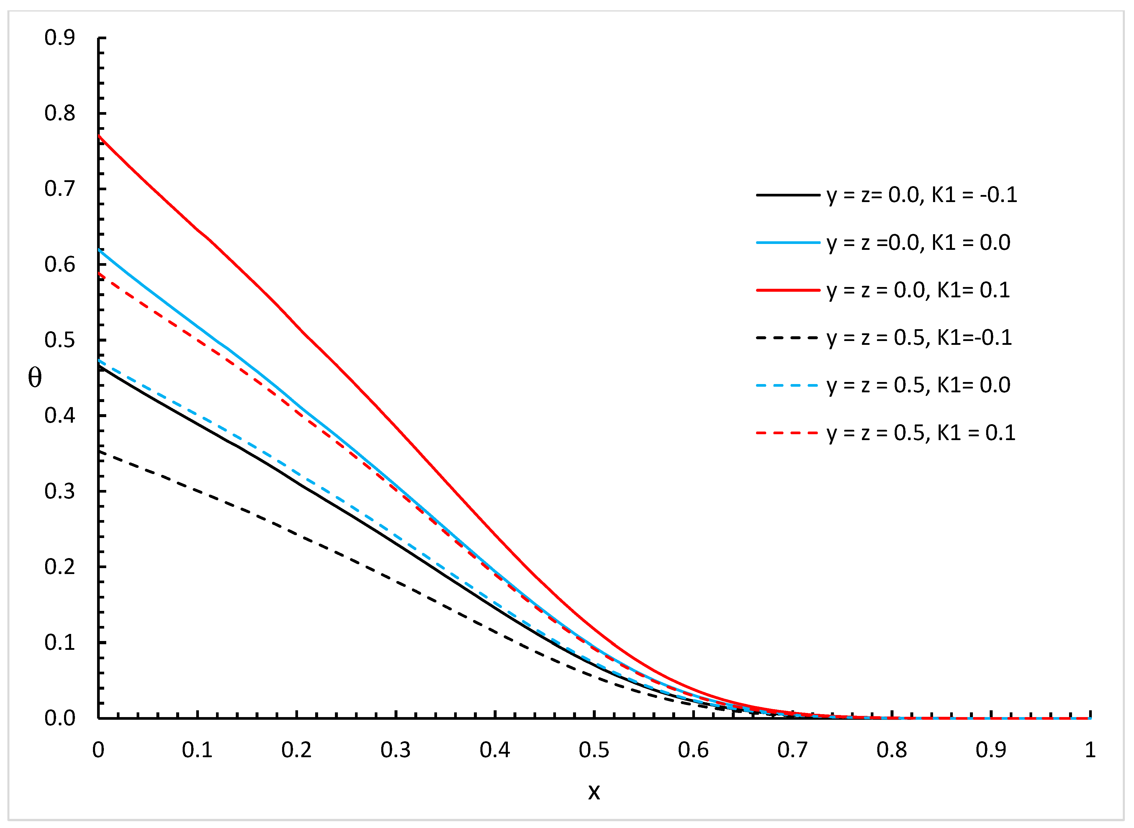
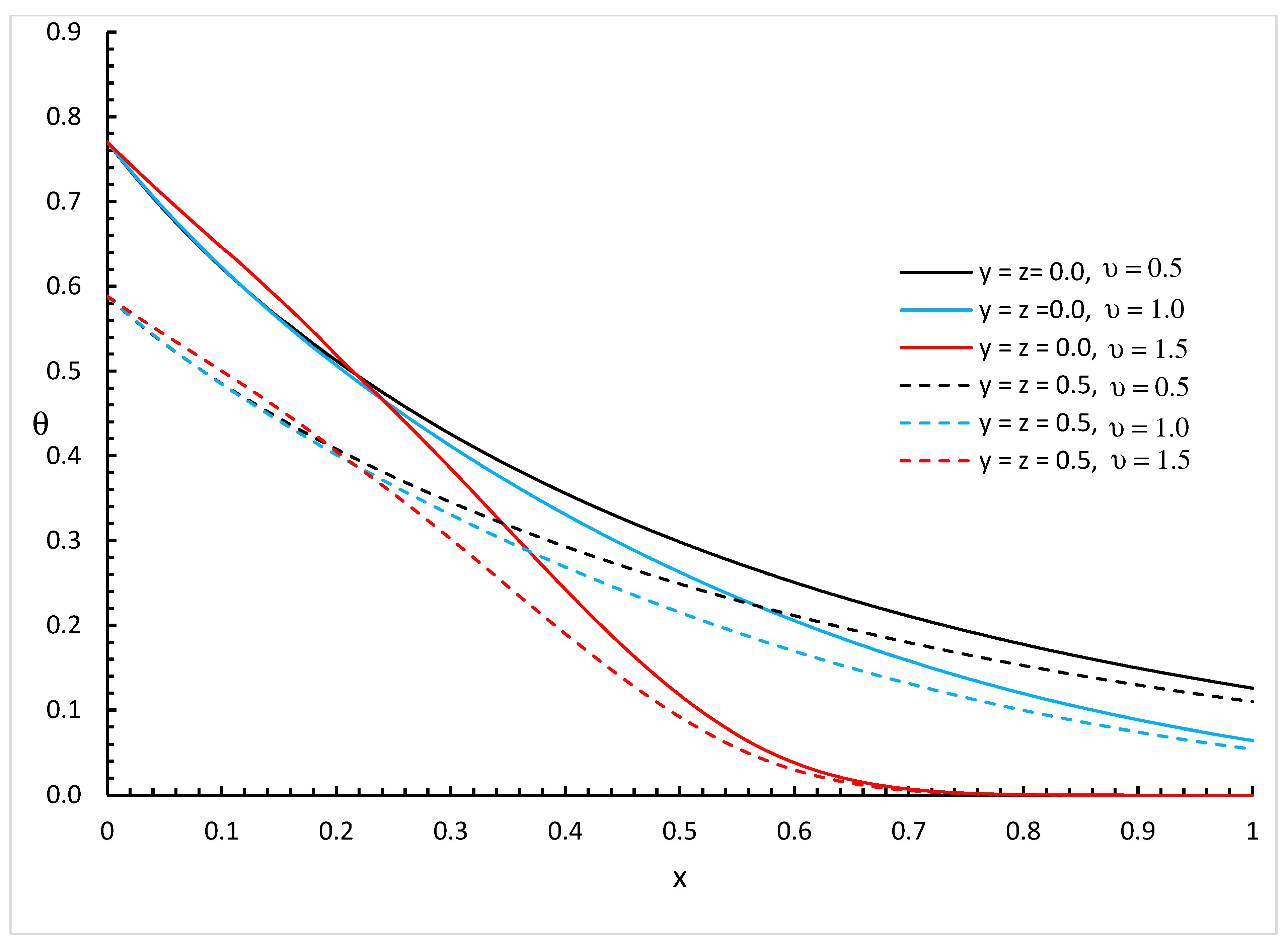
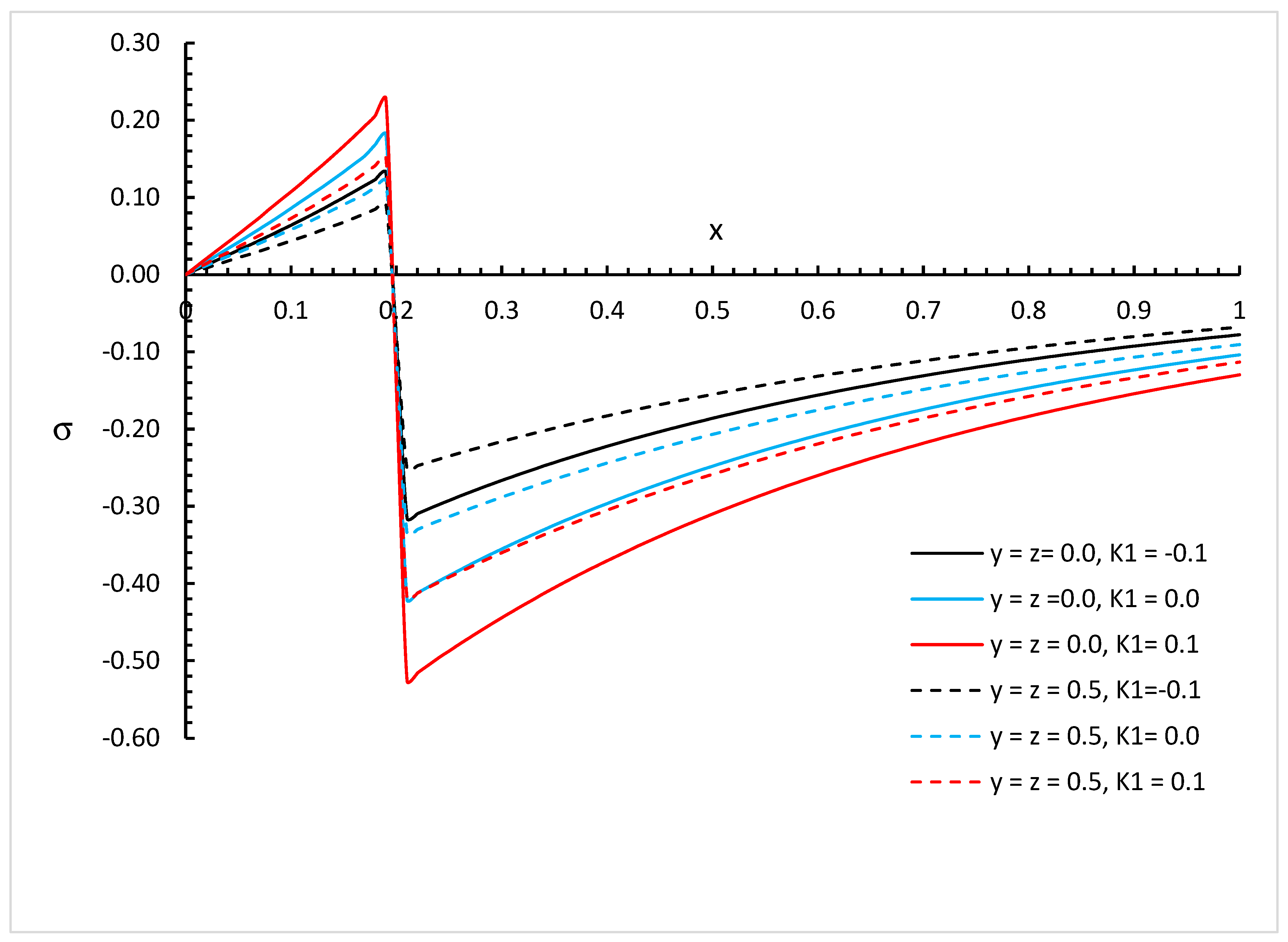
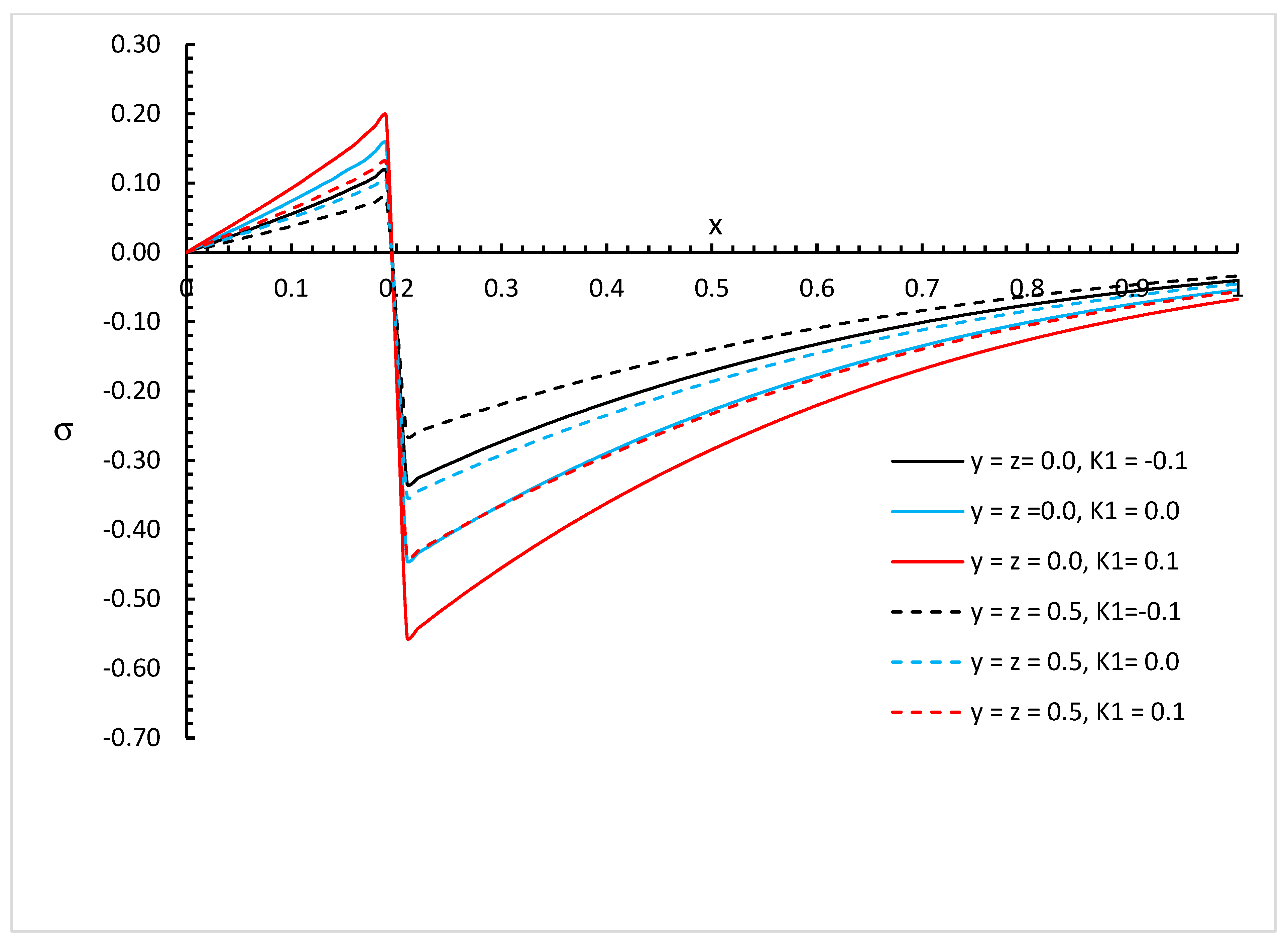
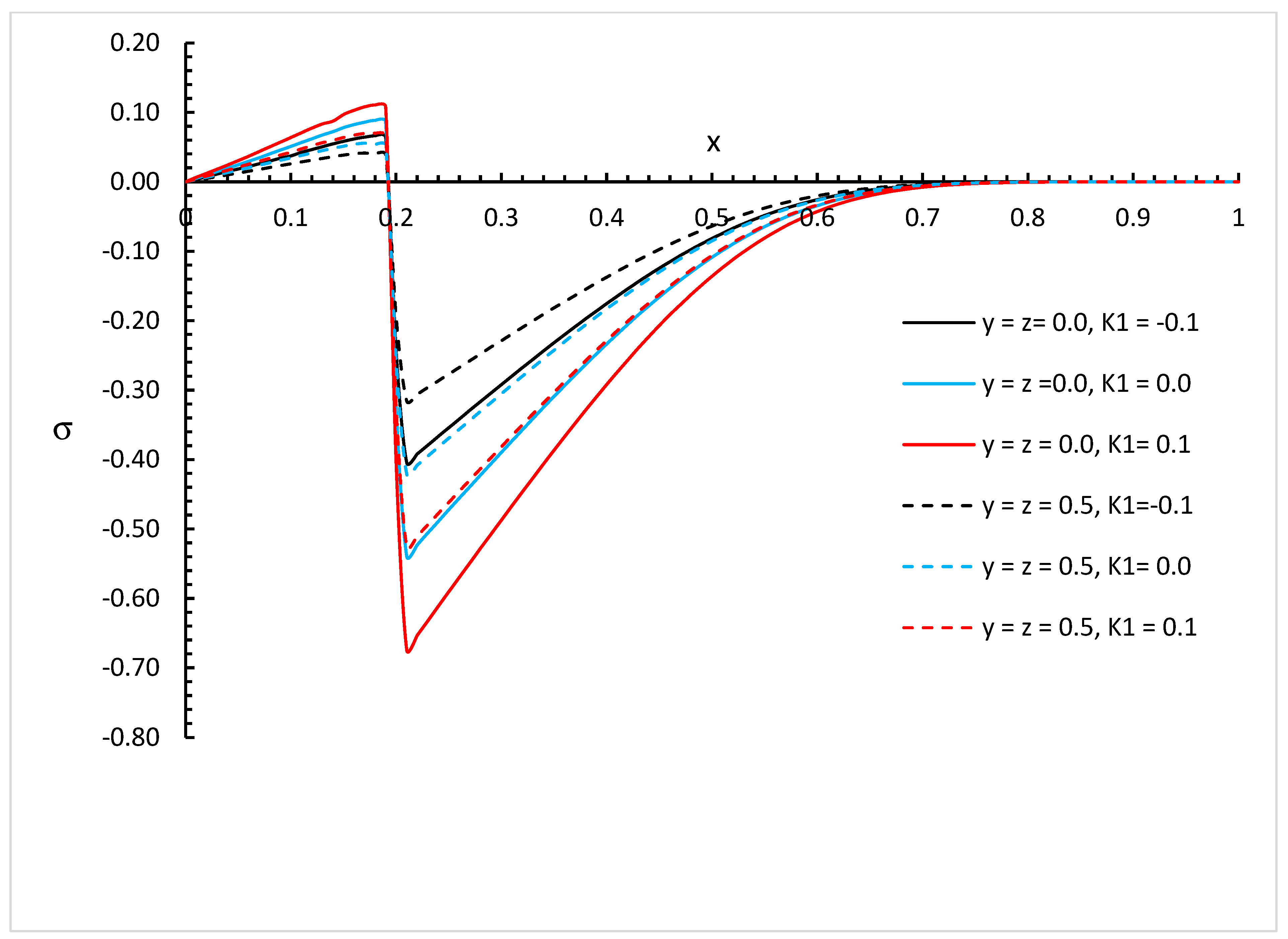
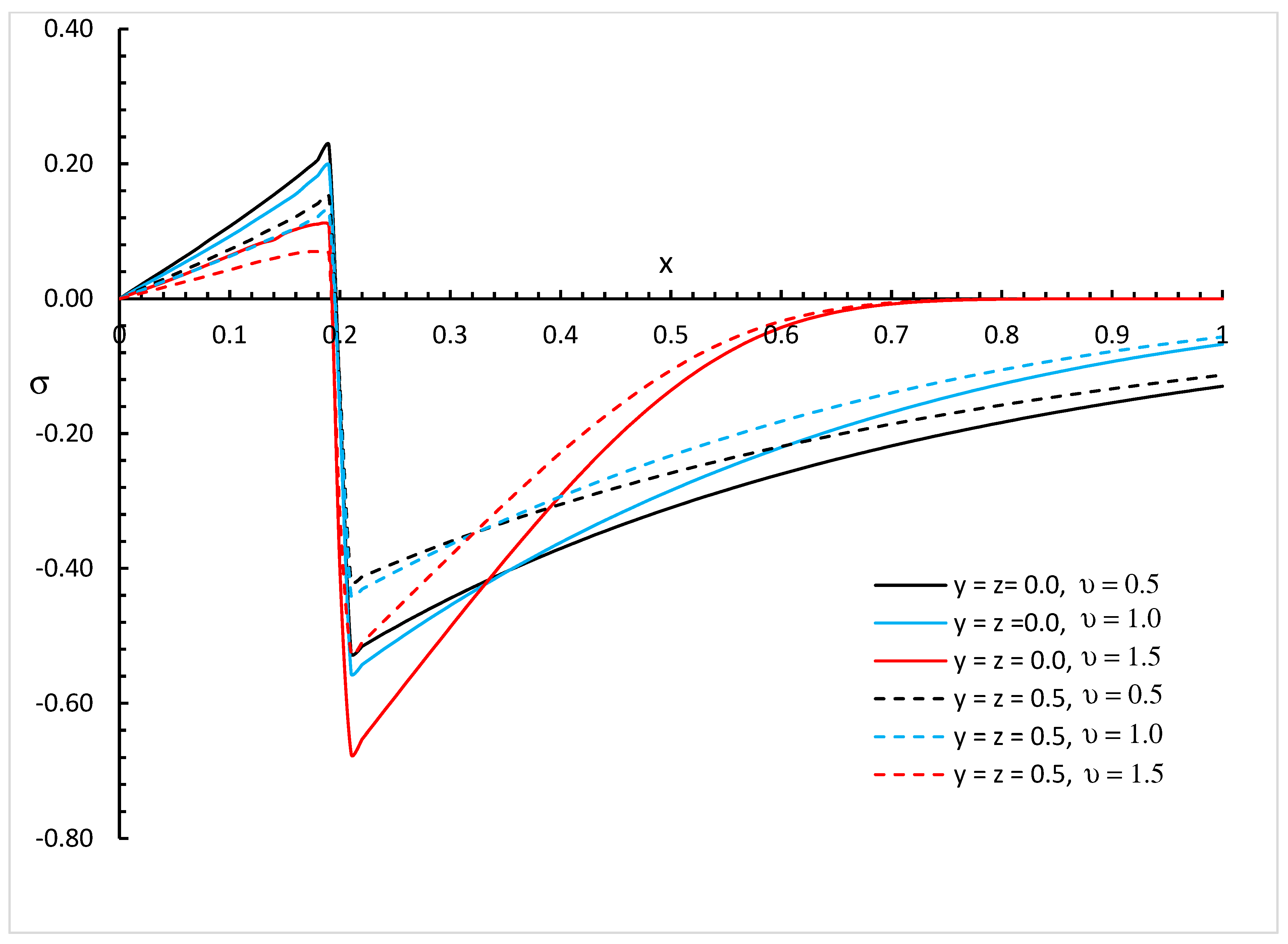
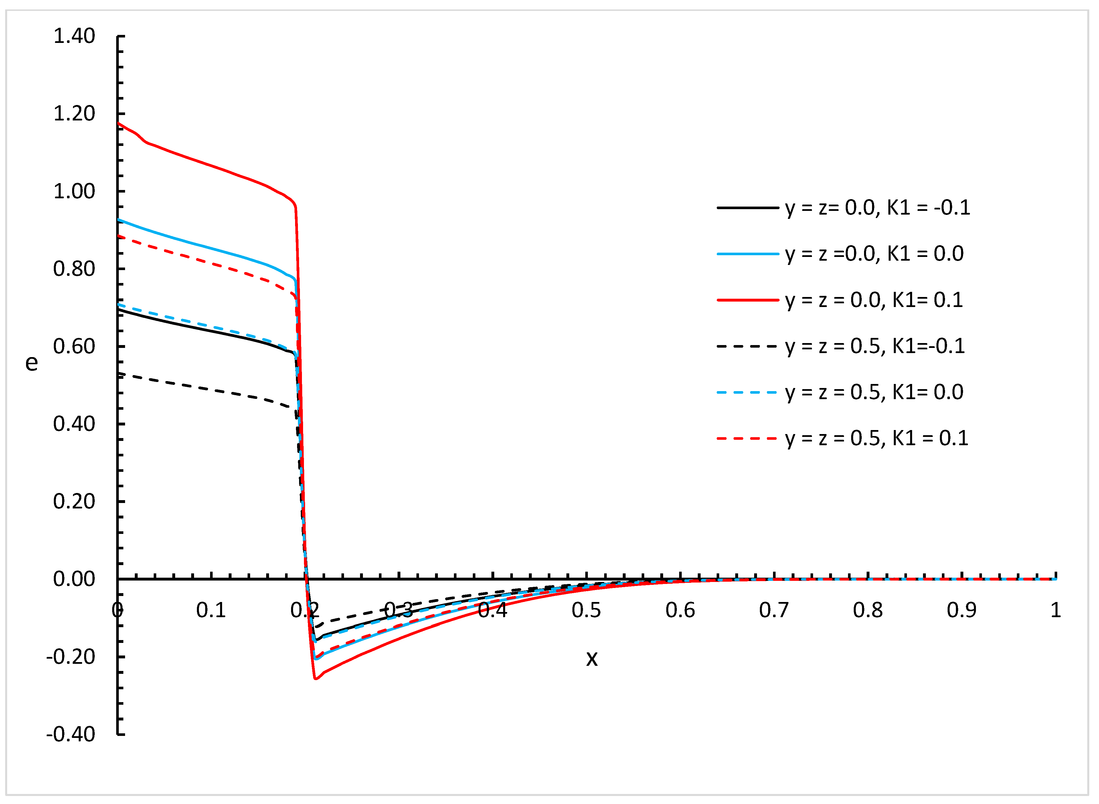
• It is noted that the value of the fractional order parameter and the variability of the thermal conductivity have significant effects on the mechanical and thermal waves.
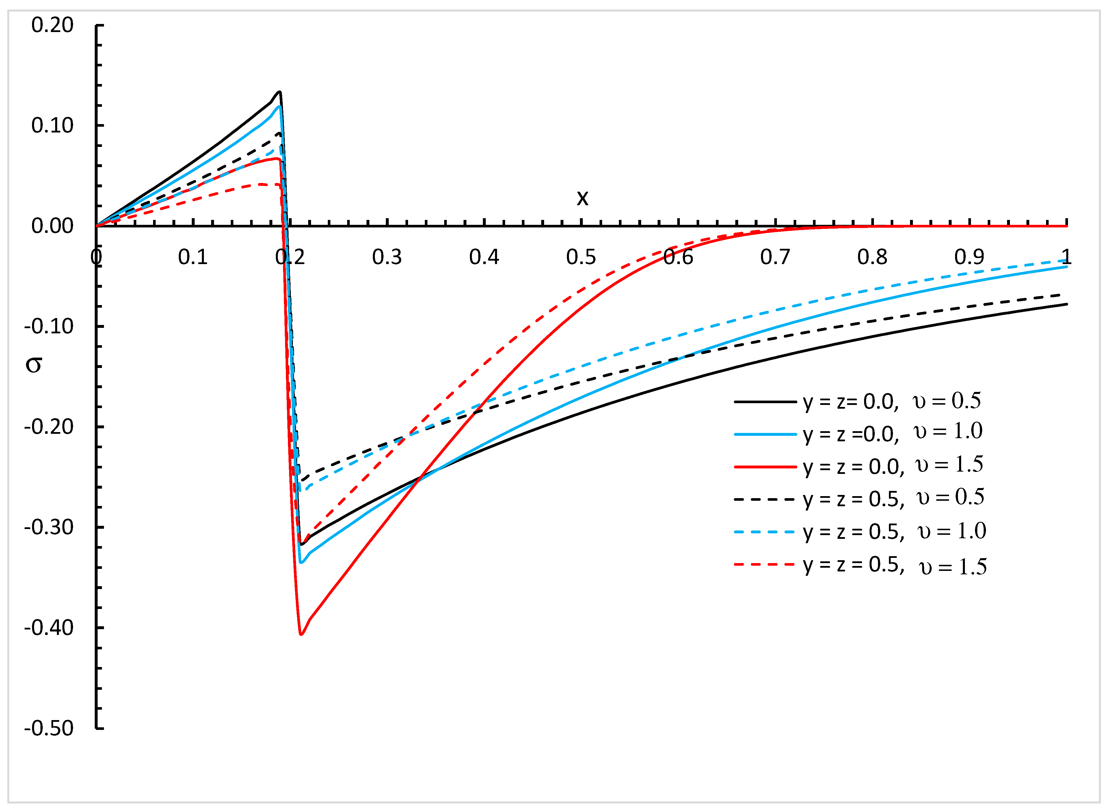
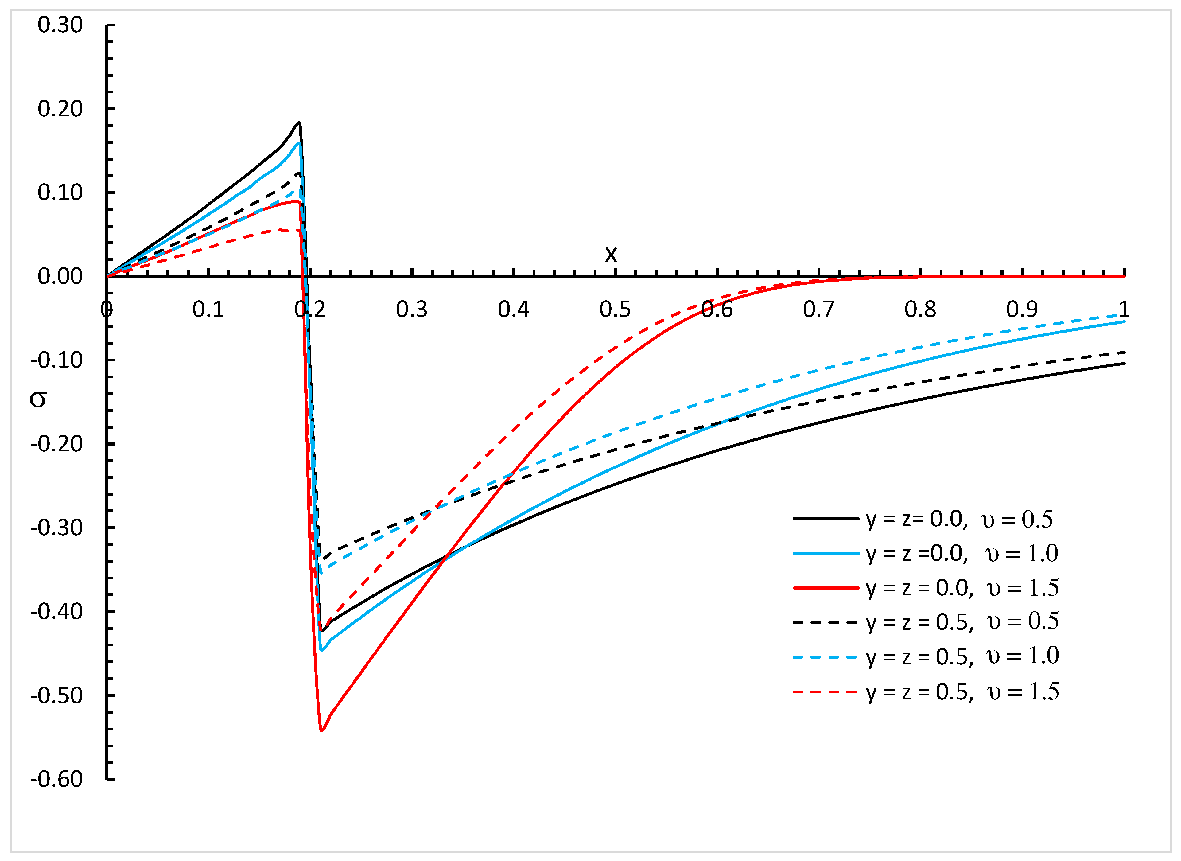
• The distributions of the temperature increment, invariant stress, and invariant strain fall to zero at a smaller distance from the bounding surface in the order of strong thermal conductivity, followed by normal thermal conductivity, and finally weak thermal conductivity.
• The results of this work agree with other works when the value of the fractional order parameter is equal to one and the thermal conductivity is constant, such as in references [18,40,43,44].
• The Moor–Gibson–Thompson model is a successful model for simulating three-dimensional thermoelastic materials with variable thermal conductivity and fractional order heat conduction.
• Classifying the thermal conductivity as weak, normal, and strong is important and close to the physical behaviour of the thermal conductivity of the thermoelastic materials.

References

1. Biot, M.A. Thermoelasticity and irreversible thermodynamics. J. Appl. Phys. 1956, 27, 240–253. [Google Scholar] [CrossRef]
2. Sherief, H.; Naim Anwar, M.; Abd El-Latief, A.; Fayik, M.; Tawfik, A. A fully coupled system of generalized thermoelastic theory for semiconductor medium. Sci. Rep. 2024, 14, 13876. [Google Scholar] [CrossRef] [PubMed]
3. Svanadze, M. On the coupled theory of thermoelastic double-porosity materials. J. Therm. Stress. 2022, 45, 576–596. [Google Scholar] [CrossRef]
4. Lord, H.W.; Shulman, Y. A generalized dynamical theory of thermoelasticity. J. Mech. Phys. Solids 1967, 15, 299–309. [Google Scholar] [CrossRef]
5. Alihemmati, J.; Beni, Y.T. Generalized thermoelasticity of microstructures: Lord-Shulman theory with modified strain gradient theory. Mech. Mater. 2022, 172, 104412. [Google Scholar] [CrossRef]
6. Hou, W.; Fu, L.-Y.; Carcione, J.M.; Wang, Z.; Wei, J. Simulation of thermoelastic waves based on the Lord-Shulman theory. Geophysics 2021, 86, T155–T164. [Google Scholar] [CrossRef]
7. Bouslimi, J.; Omri, M.; Kilany, A.; Abo-Dahab, S.; Hatem, A. Mathematical model on a photothermal and voids in a semiconductor medium in the context of Lord-Shulman theory. Waves Random Complex Media 2024, 34, 5594–5611. [Google Scholar] [CrossRef]
8. Green, A.; Lindsay, K. Thermoelasticity. J. Elast. 1972, 2, 1–7. [Google Scholar] [CrossRef]
9. Sharifi, H. Dynamic response of an orthotropic hollow cylinder under thermal shock based on Green–Lindsay theory. Thin-Walled Struct. 2023, 182, 110221. [Google Scholar] [CrossRef]
10. Karimipour Dehkordi, M.; Kiani, Y. Lord–Shulman and Green–Lindsay-based magneto-thermoelasticity of hollow cylinder. Acta Mech. 2024, 235, 51–72. [Google Scholar] [CrossRef]
11. Green, A.; Naghdi, P. On undamped heat waves in an elastic solid. J. Therm. Stress. 1992, 15, 253–264. [Google Scholar] [CrossRef]
12. Green, A.; Naghdi, P. Thermoelasticity without energy dissipation. J. Elast. 1993, 31, 189–208. [Google Scholar] [CrossRef]
13. Hendy, M.M.; Ezzat, M.A. A modified Green-Naghdi fractional order model for analyzing thermoelectric MHD. Int. J. Numer. Methods Heat Fluid Flow 2024, 34, 2376–2398. [Google Scholar] [CrossRef]
14. Jagtap, A.D.; Mitsotakis, D.; Karniadakis, G.E. Deep learning of inverse water waves problems using multi-fidelity data: Application to Serre–Green–Naghdi equations. Ocean Eng. 2022, 248, 110775. [Google Scholar] [CrossRef]
15. Danyluk, M.; Geubelle, P.; Hilton, H. Two-dimensional dynamic and three-dimensional fracture in viscoelastic materials. Int. J. Solids Struct. 1998, 35, 3831–3853. [Google Scholar] [CrossRef]
16. Ezzat, M.A.; Youssef, H.M. Three-dimensional thermal shock problem of generalized thermoelastic half-space. Appl. Math. Model. 2010, 34, 3608–3622. [Google Scholar] [CrossRef]
17. Ezzat, M.A.; Youssef, H.M. Three-dimensional thermo-viscoelastic material. Mech. Adv. Mater. Struct. 2016, 23, 108–116. [Google Scholar] [CrossRef]
18. Youssef, H.; Abbas, I. Thermal shock problem of generalized thermoelasticity for an infinitely long annular cylinder with variable thermal conductivity. Comput. Methods Sci. Technol. 2007, 13, 95–100. [Google Scholar] [CrossRef]
19. Youssef, H.M. Two-dimensional thermal shock problem of fractional order generalized thermoelasticity. Acta Mech. 2012, 223, 1219–1231. [Google Scholar] [CrossRef]
20. Hafed, Z.S.; Zenkour, A.M. Refined generalized theory for thermoelastic waves in a hollow sphere due to maintained constant temperature and radial stress. Case Stud. Therm. Eng. 2025, 68, 105905. [Google Scholar] [CrossRef]
21. Khader, S.; Marrouf, A.; Khedr, M. A model for elastic half space under a visco-elastic layer in generalized thermoelasticity. Contin. Mech. Thermodyn. 2025, 37, 25. [Google Scholar] [CrossRef]
22. Yahya, A.; Saidi, A. Response of Generalized Thermoelastic for Free Vibration of a Solid Cylinder with Voids Under a Dual-Phase Lag Model. Iran. J. Sci. Technol. Trans. Mech. Eng. 2025, 1–11. [Google Scholar] [CrossRef]
23. Li, S.; Sun, J.; Zhu, J. Analytical solution of dual-phase-lagging generalized thermoelastic damping in Levinson micro/nano rectangular plates. J. Therm. Stress. 2025, 1–19. [Google Scholar] [CrossRef]
24. Quintanilla, R. Moore–Gibson–Thompson thermoelasticity. Math. Mech. Solids 2019, 24, 4020–4031. [Google Scholar] [CrossRef]
25. Quintanilla, R. Moore-Gibson-Thompson thermoelasticity with two temperatures. Appl. Eng. Sci. 2020, 1, 100006. [Google Scholar] [CrossRef]
26. Singh, B.; Mukhopadhyay, S. Galerkin-type solution for the Moore–Gibson–Thompson thermoelasticity theory. Acta Mech. 2021, 232, 1273–1283. [Google Scholar] [CrossRef]
27. Bazarra, N.; Fernández, J.R.; Quintanilla, R. Analysis of a Moore–Gibson–Thompson thermoelastic problem. J. Comput. Appl. Math. 2021, 382, 113058. [Google Scholar] [CrossRef]
28. Fernández Sare, H.D.; Quintanilla, R. Moore Gibson Thompson thermoelastic plates: Comparisons. J. Evol. Equ. 2023, 23, 70. [Google Scholar] [CrossRef]
29. Mondal, S.; Srivastava, A.; Mukhopadhyay, S. Thermoelastic wave propagation and reflection in biological tissue under nonlocal elasticity and Moore–Gibson–Thompson heat conduction: Modeling and analysis. Z. Angew. Math. Und Phys. 2025, 76, 30. [Google Scholar] [CrossRef]
30. Kadian, P.; Kumar, S.; Sangwan, M. Influence of initial stress and gravity on fiber-reinforced thermoelastic solid using Moore–Gibson–Thompson generalized theory of thermoelasticity. Multidiscip. Model. Mater. Struct. 2025, 21, 217–238. [Google Scholar] [CrossRef]
31. Ahmed, Y.; Zakria, A.; Osman, O.A.A.; Suhail, M.; Rabih, M.N.A. Fractional Moore–Gibson–Thompson Heat Conduction for Vibration Analysis of Non-Local Thermoelastic Micro-Beams on a Viscoelastic Pasternak Foundation. Fractal Fract. 2025, 9, 118. [Google Scholar] [CrossRef]
32. Bahar, L.Y.; Hetnarski, R.B. State Space Approach to Thermoelasticity. J. Therm. Stress. 1978, 1, 135–145. [Google Scholar] [CrossRef]
33. Ezzat, M.A. State space approach to solids and fluids. Can. J. Phys. 2008, 86, 1241–1250. [Google Scholar] [CrossRef]
34. Bahar, L.; Hetnarski, R. Transfer matrix approach to thermoelasticity. In Proceedings of the 15th Midwest Mechanic Conference, Chicago, IL, USA, 15–17 May 1977; pp. 161–163. [Google Scholar]
35. Povstenko, Y.Z. Fractional heat conduction equation and associated thermal stress. J. Therm. Stress. 2004, 28, 83–102. [Google Scholar] [CrossRef]
36. Heymans, N.; Podlubny, I. Physical interpretation of initial conditions for fractional differential equations with Riemann-Liouville fractional derivatives. Rheol. Acta 2006, 45, 765–771. [Google Scholar] [CrossRef]
37. Meral, F.; Royston, T.; Magin, R. Fractional calculus in viscoelasticity: An experimental study. Commun. Nonlinear Sci. Numer. Simul. 2010, 15, 939–945. [Google Scholar] [CrossRef]
38. Youssef, H.M. Theory of fractional order generalized thermoelasticity. J. Heat Transf. 2010, 132, 061301. [Google Scholar] [CrossRef]
39. Youssef, H.M. State-space approach to fractional order two-temperature generalized thermoelastic medium subjected to moving heat source. Mech. Adv. Mater. Struct. 2013, 20, 47–60. [Google Scholar] [CrossRef]
40. Youssef, H.M.; Abbas, I.A. Fractional order generalized thermoelasticity with variable thermal conductivity. J. Vibroeng. 2014, 16, 4077–4087. [Google Scholar]
41. Youssef, H.M.; Al-Lehaibi, E.A. Fractional order generalized thermoelastic half-space subjected to ramp-type heating. Mech. Res. Commun. 2010, 37, 448–452. [Google Scholar] [CrossRef]
42. Hasselman, D.P. Thermal Stresses in Severe Environments; Springer Science & Business Media: Berlin/Heidelberg, Germany, 2012. [Google Scholar]
43. Ezzat, M.A.; Youssef, H.M. State space approach for conducting magneto-thermoelastic medium with variable electrical and thermal conductivity subjected to ramp-type heating. J. Therm. Stress. 2009, 32, 414–427. [Google Scholar] [CrossRef]
44. Youssef, H.M.; El-Bary, A. Mathematical model for thermal shock problem of a generalized thermoelastic layered composite material with variable thermal conductivity. Comput. Methods Sci. Technol. 2006, 12, 165–171. [Google Scholar] [CrossRef]
45. Mirparizi, M.; Razavinasab, S.M. Modified Green–Lindsay analysis of an electro-magneto elastic functionally graded medium with temperature dependency of materials. Mech. Time-Depend. Mater. 2021, 26, 871–890. [Google Scholar] [CrossRef]
46. Mirparizi, M.; Zhang, C.; Amiri, M.J. One-dimensional electro-magneto-poro-thermoelastic wave propagation in a functionally graded medium with energy dissipation. Phys. Scr. 2022, 97, 045203. [Google Scholar] [CrossRef]
47. Mirparizi, M.; Shariyat, M.; Fotuhi, A. Large Deformation Hermitian Finite Element Coupled Thermoelasticity Analysis of Wave Propagation and Reflection in a Finite Domain. J. Solid Mech. 2021, 13, 485–502. [Google Scholar]
48. Hetnarski, R.B.; Eslami, M.R.; Gladwell, G. Thermal Stresses: Advanced Theory and Applications; Springer: Berlin/Heidelberg, Germany, 2009. [Google Scholar]
49. Wang, X.; Shao, M.; Zhang, S.; Liu, X. Biomedical applications of gold nanorod-based multifunctional nano-carriers. J. Nanoparticles Res. 2013, 15, 1892–1913. [Google Scholar] [CrossRef]
Figure 1. The homogeneous, isotropic, thermoelastic, and three-dimensional body.
Fractalfract 09 00145 g001
Figure 2. The temperature increment distribution based on weak thermal conductivity with different values of K 1 and different positions of y , z when υ = 0.5 .
Fractalfract 09 00145 g002
Figure 3. The temperature increment distribution based on normal thermal conductivity with different values of K 1 and different positions of y , z when υ = 1.0 .
Fractalfract 09 00145 g003
Figure 4. The temperature increment distribution based on strong thermal conductivity with different values of K 1 and different positions of y , z when υ = 1.5 .
Fractalfract 09 00145 g004
Figure 5. The temperature increment distribution with various values of fractional order parameter and different positions of y , z when K 1 = 0.1 .
Fractalfract 09 00145 g005
Figure 6. The temperature increment distribution with various values of fractional order parameter and different positions of y , z when K 1 = 0.0 .
Fractalfract 09 00145 g006
Figure 7. The temperature increment distribution with various values of fractional order parameter and different positions of y , z when K 1 = 0.1 .
Fractalfract 09 00145 g007
Figure 8. The invariant stress distribution based on weak thermal conductivity with different values of K 1 and different positions of y , z when υ = 0.5 .
Fractalfract 09 00145 g008
Figure 9. The invariant distribution based on normal thermal conductivity with different values of K 1 and different positions of y , z when υ = 1.0 .
Fractalfract 09 00145 g009
Figure 10. The invariant stress distribution based on strong thermal conductivity with different values of K 1 and different positions of y , z when υ = 1.5 .
Fractalfract 09 00145 g010
Figure 11. The invariant stress distribution with various values of fractional order parameter and different positions y , z when K 1 = 0.1 .
Fractalfract 09 00145 g011
Figure 12. The invariant stress distribution with various values of fractional order parameter and different positions y , z when K 1 = 0.0 .
Fractalfract 09 00145 g012
Figure 13. The invariant stress distribution with various values of fractional order parameter and different positions y , z when K 1 = 0.1 .
Fractalfract 09 00145 g013
Figure 14. The strain distribution based on weak thermal conductivity with different values of K 1 and different positions of y , z when υ = 0.5 .
Fractalfract 09 00145 g014
Figure 15. The strain distribution based on normal thermal conductivity with different values of K 1 and different positions of y , z when υ = 1.0 .
Fractalfract 09 00145 g015
Figure 16. The strain distribution based on strong thermal conductivity with different values of K 1 and different positions of y , z when υ = 1.5 .
Fractalfract 09 00145 g016
Figure 17. The strain distribution with various values of fractional order parameter and different positions y , z when K 1 = 0.1 .
Fractalfract 09 00145 g017
Figure 18. The strain distribution with various values of fractional order parameter and different positions y , z when K 1 = 0.0 .
Fractalfract 09 00145 g018
Figure 19. The strain distribution with various values of fractional order parameter and different positions y , z when K 1 = 0.1 .
Fractalfract 09 00145 g019
Disclaimer/Publisher’s Note: The statements, opinions and data contained in all publications are solely those of the individual author(s) and contributor(s) and not of MDPI and/or the editor(s). MDPI and/or the editor(s) disclaim responsibility for any injury to people or property resulting from any ideas, methods, instructions or products referred to in the content.