Bridging the Scaling Gap: A Review of Nonlinear Paradigms for the Estimation and Understanding of Extreme Rainfall from Heavy Storms

Abstract

Short-duration extreme rainfall is a major trigger of flash floods and urban inundation, yet its quantification remains a profound challenge due to the scarcity of high-resolution observations. This review synthesizes how three central paradigms of nonlinear science, multifractal cascade theory, self-organized criticality (SOC) and chaos theory, provide critical insights and practical methodologies for bridging this observational gap. We examine how multifractal temporal downscaling leverages scale-invariance to derive sub-hourly rainfall statistics from coarser data. The SOC paradigm is discussed for its ability to explain the power-law statistics of rainfall extremes and cluster properties, offering a physical basis for estimating rare events. The role of chaos theory and its modern evolution into complex network analysis is explored for diagnosing predictability and spatiotemporal organization. By comparing and integrating these perspectives plus recent developments in stochastic hydrology, this review highlights their collective potential to advance the estimation, understanding, and prediction of short-duration extreme rainfall, ultimately informing improved risk assessment and climate resilience strategies.

1. Introduction

Extreme rainfall is one of the most disastrous natural hazards that would impact infrastructure, societal activities and even threat to lives. Many severe weather systems are sources of extreme rainfall, including thunderstorm, tropical and extratropical cyclone, fronts and monsoons. Thus, understanding the physical mechanisms of extreme rainfall generation is highly challenging. With the warming atmosphere under climate change, there is strong evidence that rain rates will increase at many timescales [1,2], although uncertainties exist on what aspects of rainfall will change in the future (e.g., its probability density function or PDF [3], variability [4,5], and dependency on temperature and moisture [6].

Rainfall is a highly intermittent process and accordingly rain accumulated at different timescales would show different characteristics. Accumulated rainfall at daily or longer timescale is useful for water management, drought assessment and climate monitoring. However, many critical hazards are due to short-duration extreme rainfall at hourly to sub-hourly timescale, such as flash flood [7] and landslide [8]. Up to recently, we still have little knowledge on how short-duration rainfall will change with the climate, which is critical to hydrological infrastructure design.

Short-duration rainfall has not been well observed by conventional gauge networks and there is spatial inhomogeneity. Radar- and satellite-based observations can supplement rain gauges at hourly and sub-hourly scale; however, they are biased especially for the extreme parts and still limited in spatial coverage. This is why in early review on short-duration extreme rainfall [9], improving statistical techniques for detecting changes was emphasized. Given the short periods of high-quality short-duration rain observations for deducing valid statistical relationships, one approach is to analyze multiple sites and examine PDFs of rainfall in a region [10] or the “space-for-time substitution”. Another approach is through temporal scaling, i.e., the concept of deriving sub-scale statistics from supra-scale data. Mathematically, whether the following scaling relationship is valid between rain intensities (I_d and I_D) within durations d and D:

$$I_d={\left({\displaystyle \raisebox{1ex}{$d$}\!\left/ \!\raisebox{-1ex}{$D$}\right.}\right)}^{-\eta }{I}_D,$$

(1)

where $\eta$ is the scaling exponent and equality is in the sense of the same statistical distribution [11]. While there has long been observational evidence that such scaling relationship is valid [11,12], factors determining the scaling exponent are obviously complex, including rainfall type, geography, environmental conditions, and its stationarity. It is also apparent that Equation (1) is closely related to construction of the Intensity-Duration-Frequency (IDF) curve that is the basis of water infrastructure design. In IDF curves, rain intensities are usually the annual maximum values with a certain frequency (return period). There is a large literature on developing various statistical techniques to construct IDF curves especially for regions without adequate gauge observations [13,14].

Another aspect is to consider rain events defined as the accumulated rainfall between commencement and termination of rain at a site, which is different from fixed-duration analysis. It is thus obvious that high-resolution observations, at least sub-daily and ideally sub-hourly, are necessary to resolve individual rain events generated by storms and convective cells. In this context, rain events have been viewed as energy cascade or relaxation processes [15,16].

Differential amplification of rain intensities at different timescales due to climate change would lead to changing relationship between rain rates with different durations. In recent hydrological studies, many different scaling relationships are the focuses. One of them is the scaling of rain intensity with air temperature or dew point temperature, which accounts for the effect of increased moisture content in the atmosphere [17]. The other types are the temporal scaling as mentioned and will be reviewed in the following also spatiotemporal scaling of rain. On many occasions, our focus is on scale invariance of certain rain-related parameters such as rain intensity and humidity (see Appendix A for mathematical definitions), implying self-similar or scale-free physical processes in behind.

Broadly speaking, three classes of models exist that can be used to describe rainfall: chaotic dynamical models, stochastic models and phenomenological models. In association with these model types, three nonlinear paradigms (although linearity is also part of them) have been developed historically to describe rainfall: multifractal cascade process, self-organized criticality and chaos theory. From different aspects, these paradigms contribute to our understanding of rainfall temporal scaling depicted above, as well as how future behavior of short-duration rain would change under the warming climate.

While there has been wealth of literature on some of the paradigms [18,19], an integrated review and discussion of them rarely exist. In this review, we emphasize the fundamentals in theories behind the paradigms, how they stemmed from earlier studies and developed to recent frontiers. Mathematical formalisms have also been provided in the appendices for reference. For researchers entering this area of science may use this review as a quick reference to a broad literature, and for experience researchers we aim to stimulate motivations to apply these nonlinear paradigms, or even cross-paradigm concepts, on atmospheric and hydrological analysis of rainfall.

2. Spectral Analysis and Spatiotemporal Scaling

2.1. Power Spectral Density (PSD) Analysis of Point Rain Rate

The point rain rate, as recorded by gauges, provides fundamental data for hydrological applications. Its variability is often studied through PDFs or power spectral density (PSD) using Fourier analysis [20]. The PSD of rain rates is a fundamental way for understanding rainfall variability. The functional form of the PSD is crucial for accurately representing the occurrence of extremes. Traditionally, the Gamma distribution has been widely used to model the highly skewed, non-negative nature of rainfall rates [21]. However, the log-normal distribution has also been proposed, particularly in the context of multiplicative cascade processes where the rain rate results from the product of many random factors [22,23]. Recent analyses continue to debate the optimal distribution; for instance, GhoshDastider et al. [24] and Lennartz and Poschlod [25] have explored these distributions in the context of scaling and extremes, while Frechen and Hinz [26] applied them to understand sub-daily rainfall statistics. The choice between Gamma and log-normal can have significant implications for the estimation of very high percentiles and the representation of intermittency.

The widespread observation of power-law PSD in rainfall, $E\left(f\right)\sim f^{-\beta }$, raises the question of its physical origin. The early interpretation, as noted, was that rain droplets act as passive tracers of 3D atmospheric turbulence, inheriting the Kolmogorov $\beta =5/3$ scaling from the inertial subrange. However, this view has been challenged. An alternative explanation posits that the scaling arises from the intrinsic dynamics of precipitation systems themselves, governed by nonlinear moisture and convection processes such as microphysical processes, rather than being a passive reflection of the turbulent velocity field [27]. The scaling exponent $\beta$ can thus be seen as an emergent property of the precipitation field’s spatiotemporal organization, linking it to the multifractal and self-organized criticality (SOC) paradigms discussed later.

High-resolution rain gauge data from the 1990s confirmed approximate Kolmogorov scaling for timescales of tens of minutes to hours [28,29,30,31]. At smaller scales (7–15 km), Crane [28] and Veneziano et al. [32] reported a transition to scaling, consistent with enstrophy cascades in 2D turbulence theory [33], likely driven by convective clusters. A further transition to scaling at ~3–7 km was also noted, although data resolution limited confirmation. Below ~2 km, mesoscale scaling may re-emerge when turbulence scale becomes comparable to the three-dimensional circulation. These transitions remain to be rigorously tested with modern observations. For example, Dimitriadis et al. [34] examined 10-s resolution rainfall intensity time series and found that the variance drops substantially at the smallest timescales (~10 s to 3 h, see Figure A1c in [34]) and deviates from power-law scaling.

At second-level resolution, Fabry [35] found a near-white noise spectrum, attributed to hydrometeor fall speeds. Conversely, at multi-year timescales, Fabry [35] and Fraedrich and Larnder [36] observed spectral plateaus (i.e., $f^0$) with little evidence of scaling, suggesting rainfall variability resembles white noise at climatic scales.

Environmental controls on PSD scaling are less clear. Harris et al. [37] found systematic dependence of the scaling exponent on altitude in New Zealand, though later studies using radar reflectivity [38] showed little altitude effect. Stratiform and convective rain exhibited Kolmogorov-type scaling with transitions to near-white noise at small timescales, but convective near-surface spectra sometimes showed steeper forms. Villarini et al. [39] concluded that larger multi-regime datasets are needed to resolve orographic influences.

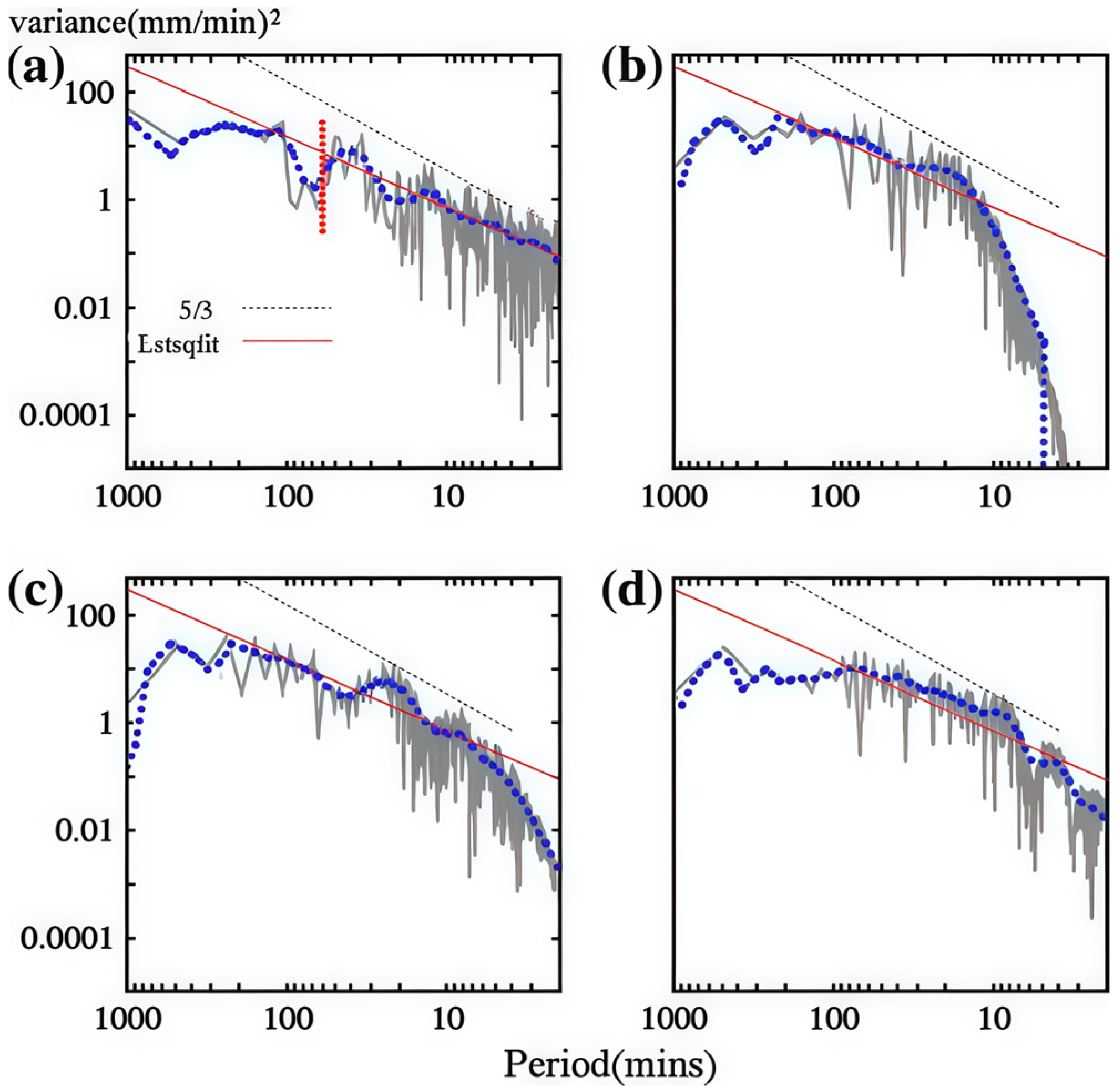
Case studies of tropical storms also reveal variability. Koh et al. [40] analyzed the December 2006 Malay Peninsula storm with 1- and 5-min gauge data (Figure 1). A scaling regime between 2–60 min yielded an exponent near 2, consistent with theoretical raindrop number density arguments [41]. They suggested that tropical storms may exhibit narrow raindrop size distributions (i.e., small variability in them) and characteristic terminal velocities, producing such scaling.

In summary, PSD studies confirm that rainfall exhibits scale-dependent behavior across wide temporal ranges, with transitions linked to turbulence regimes, storm dynamics, and possibly orography. While broad scaling laws exist (albeit exceptions such as that identified in Dimitriadis et al. [34], their universality remains debated. A recent global-scale investigation of stochastic similarity in hydrological processes [42] represented some major advancements. Based on Hurst-Kolmogorov dynamics and examination of thousands of station observations, the study confirmed universal scaling structures from fractal behavior at small scales to long-term persistence at large scales and transient behavior in between. These scaling structures apply to parameters such as surface temperature and pressure, humidity, precipitation, streamflow and winds, and thus a universal stochastic view of hydrological cycle is plausible. Improved resolution from modern sensors offers opportunities to reassess these transitions and better constrain scaling exponents, which underpin multifractal and SOC interpretations of rainfall.

2.2. Spatiotemporal Scaling

Rainfall is intermittent not only in time but also in space, and representing this spatial variability is essential for forecasting and hydrological applications. Researchers have long examined the scaling of rainfall fields to understand their structure and simulate them realistically.

As with temporal scaling, a 2D random field is scaling when with scaling exponent. Studies of water vapor and cloud fields [43,44] reported exponents slightly steeper than $\beta ={\displaystyle \frac{5}{3}}$, with breaks near 10–100 km. These results suggest mono-fractal properties, though multifractal approaches reveal additional details of intermittency and smoothness (see Appendix B for discussion on spatial moments scaling).

Numerous studies have reported similar scaling exponents. Nastrom and Gage [45] and colleagues analyzed airline humidity data (150–3000 km) and found Kolmogorov slopes at small scales (<500 km) and steeper slopes at larger scales. Radar data from New Zealand showed exponents around 2.38 across 240 m–30 km [31]. Nykanen and Harris [46] reported exponents of 2.29–2.69 for U.S. storms, with scaling ranges decreasing at higher elevations. In contrast, Cho et al. [47] found lower values (1.46–1.79) in tropical and extratropical aircraft observations, highlighting geographic dependence. Such variability suggests that local environment strongly modulates scaling.

Dynamic scaling links temporal and spatial variability. Venugopal et al. [48] showed that rainfall evolution remains invariant under space–time transformations of power-law form (where $t$ represents time scale and $L$ spatial scale):

$$t~L^z,$$

(2)

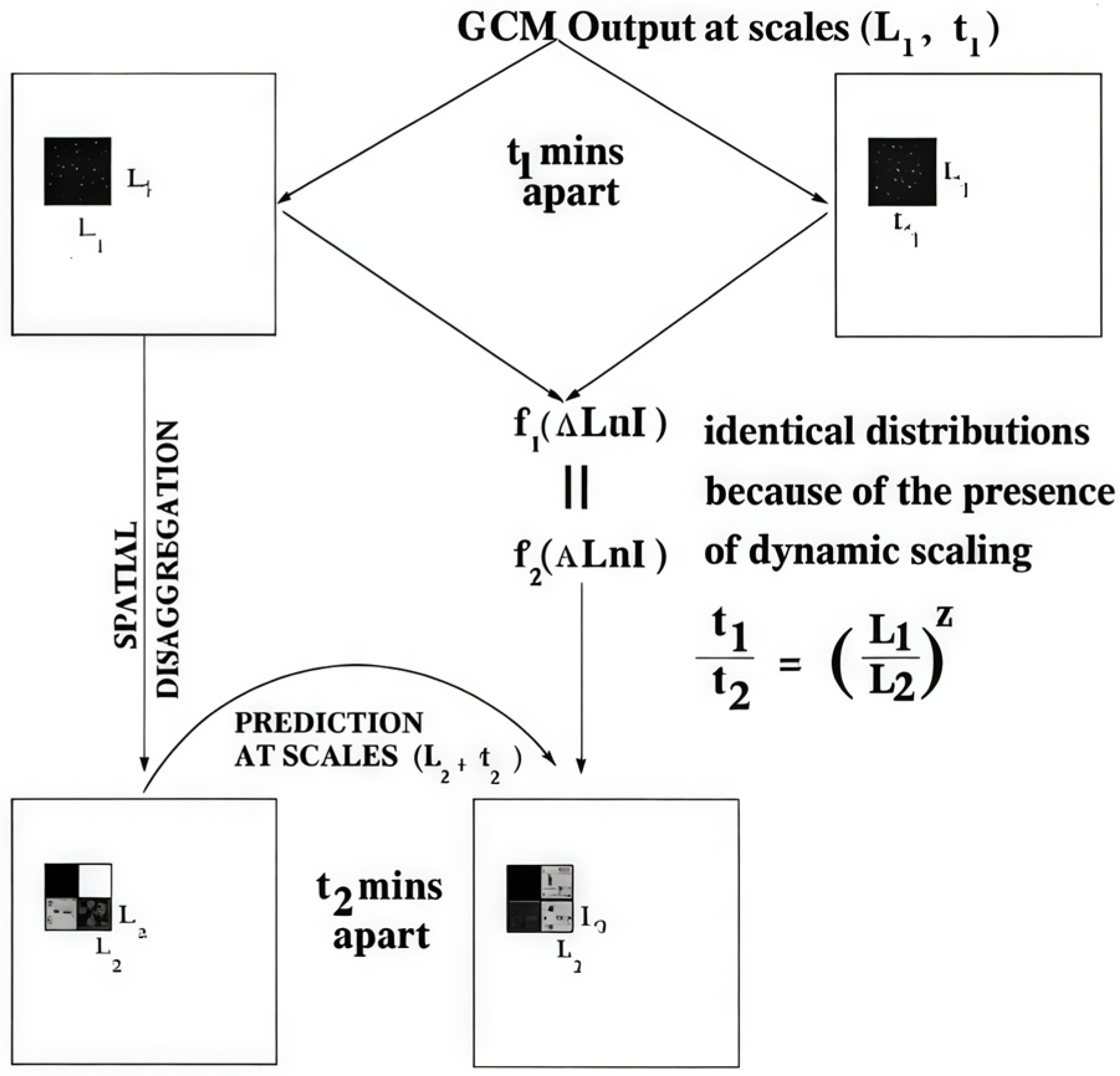
implying that statistical structures of rainfall are preserved under rescaling. They applied this framework to tropical convective storms near Darwin and termed it “dynamic scaling.” The concept was later used for downscaling models [49,50,51]. Essentially the new downscaling model examines the temporal fluctuation of the logarithm of rainfall under length scale $L$ at a specific location $(i,j)$ and time $\tau$, i.e., $∆ln{R}_{i,j,\tau }\left(L,t\right)=ln\left(R_{i,j}^L\left(\tau +t\right)\right)-ln\left(R_{i,j}^L\left(\tau \right)\right)$. By varying the length scale $L$ and time scale $t$, the statistics of this quantity can be formed by collecting data over different times and locations, assuming stationarity in space. Then, dynamic scaling refers to the fact that the PDF of $∆ln{R}_{i,j,\tau }\left(L,t\right)$ is invariant under the transformation of ${\displaystyle \raisebox{1ex}{$t$}\!\left/ \!\raisebox{-1ex}{$L^Z$}\right.}=constant$. By examining the statistics of such log-transformed rainfall across scales, these models generate consistent small-scale rainfall fields from larger-scale inputs, preserving temporal persistence and spatial coherence (Figure 2).

The “space-for-time” approach, leveraging spatial data to infer temporal trends, is a powerful tool in climatology, especially for projecting changes in short-duration extremes [9]. The dynamic scaling framework provides a physically based, stochastic method to implement this concept. By assuming the invariance of rainfall evolution statistics under power-law scaling, it allows for the generation of high-resolution, spatially coherent rainfall fields from coarser model outputs or reanalysis data. This is particularly valuable for climate impact studies where the “space-for-time” substitution, based on which rainfall scaling relationships can be deduced and extended to their temporal variations, is used to understand future flood risks in a warming climate [13].

In summary, spatiotemporal scaling analyses reveal consistent power-law behavior but also regional variability in scaling exponents. Dynamic scaling provides a bridge between spatial and temporal domains, enabling practical downscaling methods. Future research should focus on linking scaling parameters to storm type, geography, and climate regime, thereby refining stochastic downscaling tools for hydrological design and climate impact assessment.

2.3. The Climacogram Framework

The paradigms discussed thus far primarily characterize scaling through power spectra and structure functions. A complementary perspective from stochastic hydrology emphasizes the unified modeling of both the marginal statistical distributions and the dependence structures across scales. A central tool in this framework is the climacogram [52], which plots the variance of a process averaged over timescales as a function of that timescale. Under this framework, Papalexiou [53] and Papalexiou and Serinaldi [54] developed a unified theory for stochastic modelling of hydroclimatic processes that explicitly preserves pre-specified marginal distributions for intermittent processes like rainfall and correlation structures. This approach is crucial for simulating realistic rainfall fields because it ensures that not only the scaling of moments but also the full probability distribution, including the extremes, is consistent across scales. This directly addresses a key challenge in downscaling: generating high-resolution data that statistically resembles observations.

As aforementioned, Dimitriadis et al. [42] conducted a comprehensive investigation of stochastic similarity across key hydrological-cycle processes, including precipitation, and confirmed universal scaling structures. This universal stochastic framework posits that these scaling regimes are emergent properties of the underlying complex dynamics, providing a holistic view that connects the fractal turbulence discussed in Section 2.1 with the long-memory processes evident in climate records. This perspective, such as the spatiotemporal random fields model in Papalexiou and Serinaldi [54], complements the dynamic scaling of Section 2.2 by offering a stochastic, foundation for the “space-for-time” substitution, arguing that the inherent scaling laws of the hydrological cycle are robust and can be leveraged for prediction and simulation in ungauged basins.

3. Multifractal Cascade Theory

3.1. Multifractal Cascade Models

Multifractal cascade theory provides a framework for understanding rainfall variability across scales. It stems from turbulence research, where multiplicative cascades describe how energy transfers from large to small eddies. Applied to rainfall, the theory posits that storm systems redistribute moisture hierarchically, generating spatial variability at multiple scales with multifractal structures.

Early rainfall analyses identified signatures of multifractality in gauge and radar records [55,56,57], noting that single scaling exponents could not capture the observed intermittency and clustering of rain. Instead, rainfall fields display a spectrum of scaling behaviors characterized by structure functions of different orders [58]. These multifractal properties link directly to the heavy-tailed distributions and bursts of intensity typical of short-duration extremes.

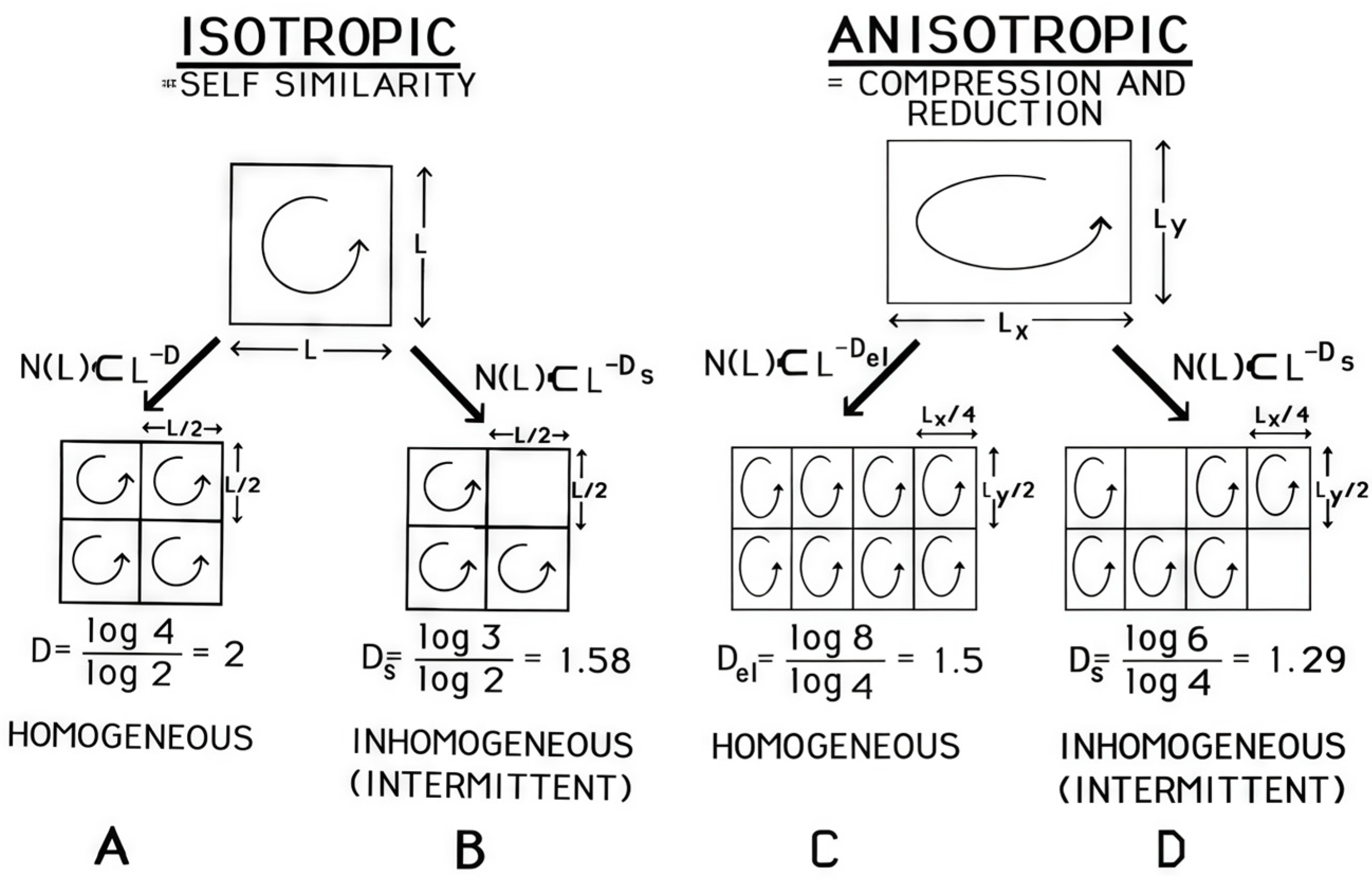
Cascade models conceptualize rainfall as the result of a hierarchical process. They began as simple isotropic models and evolved into more realistic anisotropic and inhomogeneous versions to better capture the intermittent, clumpy structure of rain fields (Figure 3) [58,59]. A key theoretical development was the shift from additive to multiplicative cascades [60,61]. While additive models generate simple, mono-fractal structures, multiplicative models reflect the underlying nonlinear dynamics of the atmosphere and produce multifractal fields, which require a spectrum of exponents to characterize their scaling properties and are a better match for observations, ranging from those in-situ to satellite-based [62,63,64,65,66,67,68].

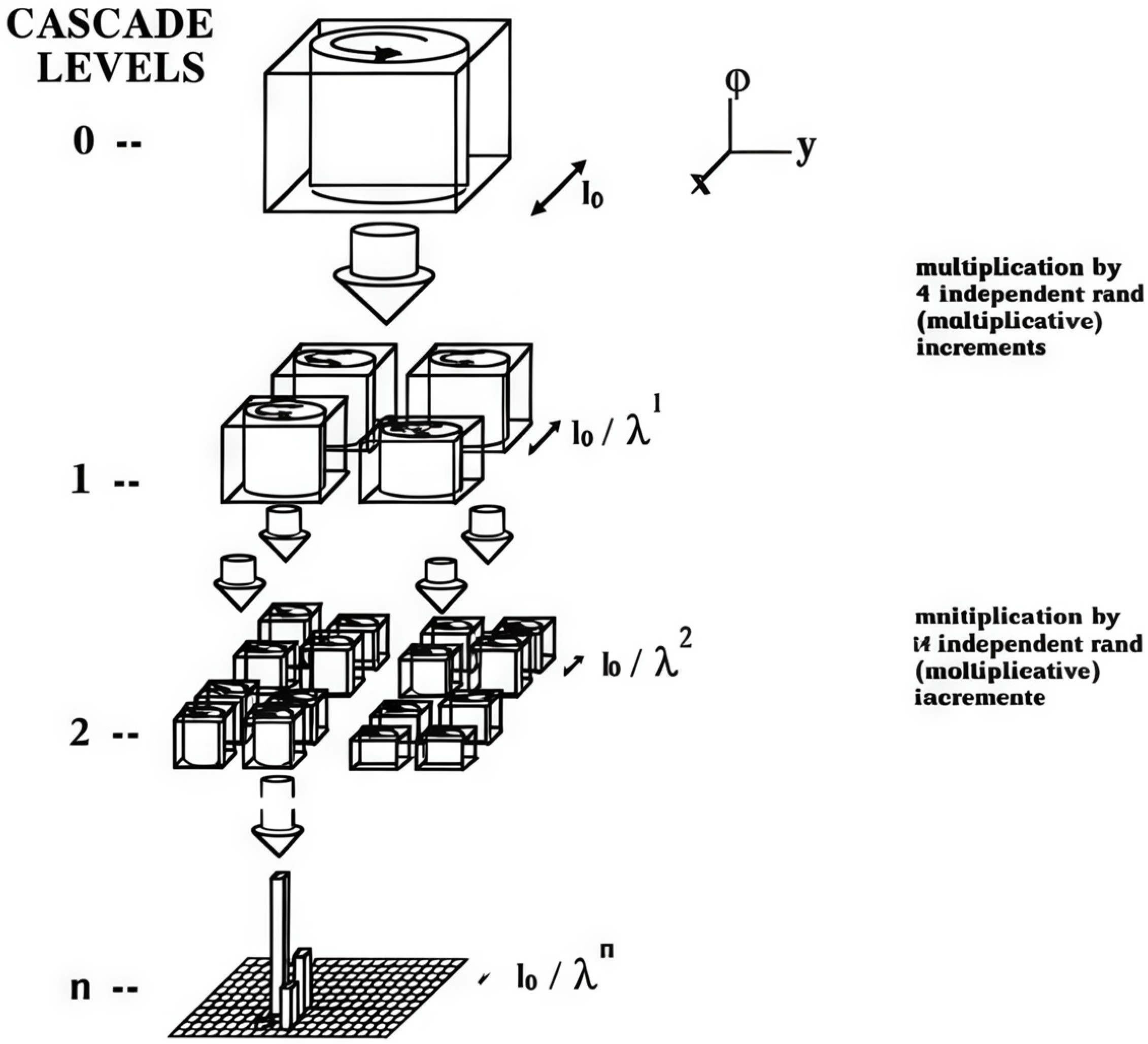
The process of a simple, conserved multiplicative cascade involves starting with a uniform rainfall flux over a large area and iteratively breaking it down into smaller sub-regions. At each step, the flux in a parent region is distributed to its children by multiplying it with a random weight, or “multiplier” (denoted as $w_i,i=1,\cdots ,2^N$ where N is number of stages [69]). Repeating this process over many steps generates a highly intermittent field with statistical properties that follow specific scaling laws, characterized by a partition function of order $q$, $M_q\left(\epsilon \right)$, where $\epsilon$ is the length scale (i.e., $2^{-N}$ at stage $N$ if the length scale starts from unit length [70]), is related proportional to the $q^{th}$ moment, ${\mu }_q$:

$$M_q\left(\epsilon \right)={\sum }_i^{2^N}{w_i}^q=2^N{{\mu }_g}^N,$$

(3)

As in Equation (A6), we expect that the partition function is following a similar scaling law in the limit as the length scale ε approaches zero, or practically after many stages of cascades:

$$M_q\left(\epsilon \right)~{\epsilon }^{\tau \left(q\right)},$$

(4)

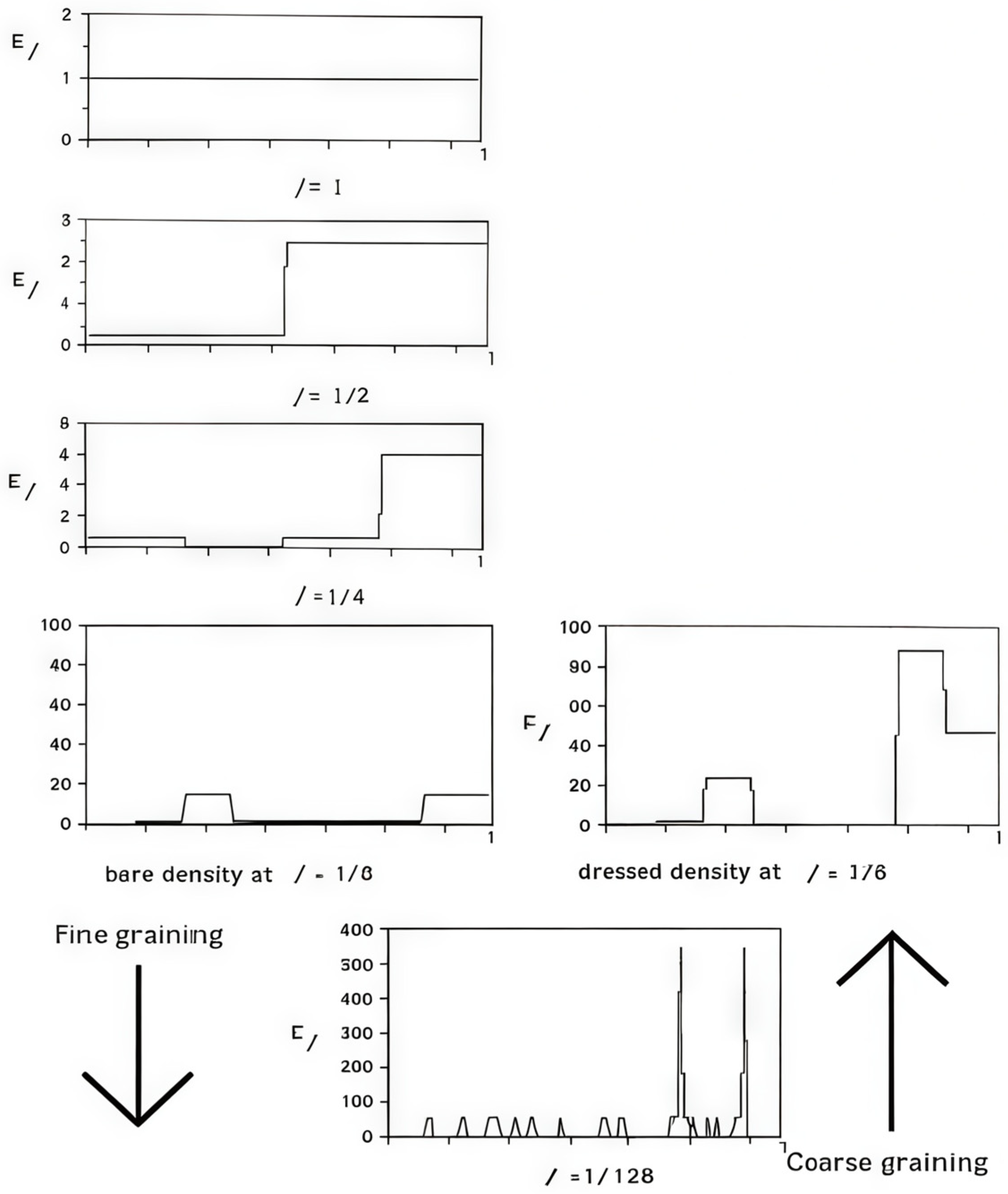
Intuitively, positive (negative) moments emphasize larger (smaller) values among the weights w_i, and thus larger absolute value of the moment magnifies intermittency and the severity of extreme events in the model realization. A crucial distinction is made between the theoretical, infinitely resolved “bare” density and the observable, coarse-grained “dressed” density, which is what practical measurements capture (Figure A2). The so-called “co-dimension multifractal formalism” [71] is discussed in Appendix C.

Applications of cascade models extend beyond pure theory. They underpin stochastic rainfall generators [72], subgrid parameterizations in numerical weather prediction, and scaling relationships for IDF curves [73]. For example, cumulus parameterization schemes in global climate models often struggle with variability at sub-daily timescales [74]. Embedding cascade concepts helps capture intermittency and clustering of convection [75], improving realism in simulated precipitation.

Theoretical developments include the universal multifractal framework, where a few parameters (such as intermittency and multifractality strength) summarize rainfall scaling across scales. These parameters provide compact descriptors of storm structure, with implications for climate projections. Observational studies have demonstrated multifractal signatures in both midlatitude and tropical regimes, though parameter values vary with geography, storm type, and measurement technique.

Recent research continues to refine and apply cascade models. Studies have focused on improving the estimation of cascade parameters from empirical data [76,77] and applying them to temporal disaggregation, a critical task for hydrological design [78,79]. Furthermore, the paradigm is being extended, for example, by analyzing rainfall from a supradroplet scale perspective [80] and revisiting the fundamental statistical properties of multiplicative cascades in geophysics [81]. Despite their utility, cascade models face challenges. A key issue is the “dressing” problem, where the transition from the theoretical, infinitely resolved “bare” cascade to the observable, spatially or temporally averaged “dressed” cascade can lead to biases in parameter estimation and the representation of extremes [82]. Furthermore, the assumption of universal scaling, while powerful, may break down in complex terrain or for specific storm types, requiring model adaptations [83].

3.2. Applications

Applications of multifractal cascade models to rainfall have been broad, ranging from statistical characterizations to practical hydrological modeling [66,84,85]. Early studies applied cascades to radar rainfall data, demonstrating that the observed clustering and intermittency of rainfall could be captured with a small number of parameters. Ong [86], for example, analyzed high-resolution gauge data and showed that cascade-based models outperform simple scaling laws in reproducing sub-hourly extremes, reinforcing their value in IDF estimation.

A widely cited contribution was Tuck [87], which drew parallels between multifractal scaling in rainfall and other atmospheric processes, linking precipitation to broader turbulence and transport phenomena. More recently, Tuck [88] updated this perspective with a synthesis of nonlinear processes in the atmosphere, emphasizing their universality across meteorology, chemistry, and dynamics. The later work highlighted that rainfall cascades should not be studied in isolation but viewed as part of a coupled system of chaotic and scale-invariant processes. This updated framing underscores the importance of using cascade theory not just as a statistical tool but as a unifying conceptual bridge across atmospheric science disciplines.

Recent practical applications include rainfall disaggregation for hydrological models, where cascade-based algorithms downscale daily totals into sub-hourly intensities that preserve intermittency. Such approaches have been used to generate synthetic extreme events for flood risk studies and to evaluate the resilience of urban drainage systems under climate change scenarios. In climate modeling, cascade concepts have been incorporated into stochastic parameterizations of convection, improving the representation of rainfall variability in both weather prediction and global climate models.

In summary, multifractal cascade theory has proven effective for reproducing rainfall intermittency, characterizing IDF relationships, and improving model parameterizations. The progression from early statistical applications to broader dynamical interpretations [87,88] illustrates the evolving role of cascades as both a practical tool and a conceptual framework connecting rainfall processes to the wider spectrum of atmospheric nonlinearities.

3.3. Current Challenges

Despite its successes, multifractal cascade theory faces several open challenges. A major issue is parameter estimation. While universal multifractal models summarize rainfall variability with a few parameters, values often differ across regions, seasons, and storm types, raising questions about universality and transferability [89]. Calibration also requires long, high-resolution datasets that are not always available, particularly in data-sparse regions.

Another challenge is linking statistical descriptors to physical processes [90,91]. Cascade models reproduce scaling and intermittency but often lack explicit connections to storm dynamics, such as convection organization, microphysics, and large-scale circulation [92,93]. Without such links, it remains difficult to interpret parameter variations in terms of underlying physics.

Modeling extremes also remains problematic. While cascades generate heavy-tailed distributions, extrapolating to rare events carries large uncertainty. Hybrid approaches that combine cascade statistics with extreme value theory or process-based models may provide more robust estimates. Similarly, downscaling applications must address non-stationarity in a changing climate, where cascade parameters may shift with warming [94].

In summary, current challenges lie in parameter universality, physical interpretability, extreme event modeling, and cross-paradigm integration. Addressing these will require high-resolution observations, process-oriented experiments, and collaborative methods that link nonlinear theory with operational hydrological applications.

4. Self-Organized Criticality and the Statistics of Extremes

SOC offers a compelling paradigm for atmospheric convection, modeling it as a system that naturally evolves to a critical state where energy input (e.g., surface heating and moisture flux) is balanced by episodic, avalanche-like releases (precipitation events). In this state, the system exhibits power-law statistics for event size and duration without any external tuning [95] (Appendix D). This is consistent with observed rainfall statistics, where the distributions of rain event sizes, durations, and dry spell lengths often follow such scaling laws [15,96,97,98].

Applied to precipitation, SOC predicts scale-free event distributions and clustering across timescales. Peters and Christensen [15,16] demonstrated that rainfall events exhibit power-law distributions of event size and duration, consistent with critical dynamics. Such behavior aligns with observations of heavy-tailed rainfall probability distributions and suggests that extremes are not outliers but intrinsic features of the rainfall process.

Statistical analysis under SOC has focused on distributions of rain event intensity, duration, and inter-event intervals. Many studies reported that cumulative distributions follow power laws over certain ranges, though exponents vary by climate regime and data resolution. Radar and gauge records reveal scaling across minutes to hours, while satellite datasets indicate persistence up to synoptic scales. These findings imply that rainfall extremes can emerge from the same organizing principles as ordinary events, with no fundamental separation between scales.

A significant application of the SOC paradigm is in providing a physical basis for Extreme Value Theory (EVT). For example, Koutsoyiannis ([52], see their Chapter 6) has extensively investigated marginal extreme value models and found that a kind of modified Pareto-Burr-Feller (PBF) distribution offered good fit to observational rainfall data within a wind range of return period (from days to hundreds of years). While traditional EVT is a statistical framework for estimating the probability of rare events, SOC offers a dynamical mechanism for why such power-law-tailed distributions might arise in the first place. Within this framework, the most extreme events, sometimes termed “dragon-kings,” can be interpreted as system-wide avalanches that are part of the same physical process that generates smaller events, rather than being statistically distinct outliers [99]. This perspective allows for the estimation of the probability of extreme, rare rainfall events based on the understanding of the system’s critical point and its associated scaling exponents, potentially improving risk assessment for catastrophic floods.

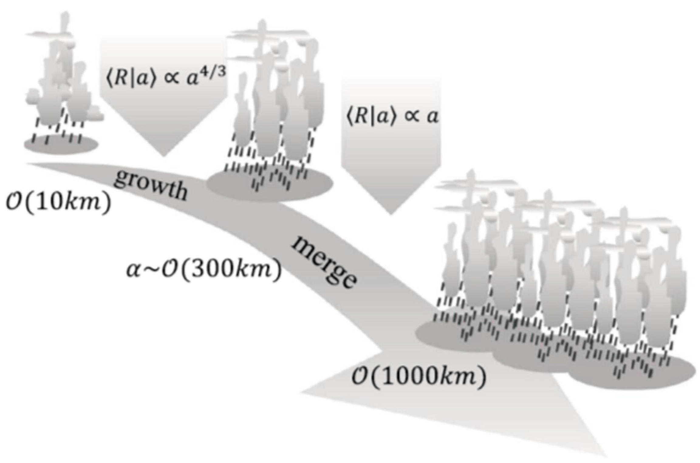
From a modeling standpoint, SOC complements multifractal and chaos frameworks. While multifractals emphasize multiplicative variability and chaos highlights deterministic instability, SOC explains the spontaneous emergence of scale-invariant behavior. Examples include the convective cloud field model in Nober and Graf, Graf and Yang [100,101], the stochastic multi-cloud model (SMCM) in Peters et al. [102] and Teo et al. [103] applied the SOC paradigm to analyze oceanic rain clusters using multi-satellite rain estimate. They estimated that the scaling exponents for cluster area and cluster total rain rate are approximately ${\displaystyle \raisebox{1ex}{$5$}\!\left/ \!\raisebox{-1ex}{$3$}\right.}$ and ${\displaystyle \raisebox{1ex}{$3$}\!\left/ \!\raisebox{-1ex}{$2$}\right.}$, respectively, which universally apply to all tropical oceanic regions. Moreover, it was argued that these two scaling exponents are related through a parameter, which represents the transitional behavior in the conditional mean of total rain rate R given a certain total rain area A of a rain cluster (Figure 4). Such transitional behavior is quite common in SOC systems [104], although not well reproduced in numerical models [105].

In summary, SOC frames rainfall extremes as natural outcomes of a self-organized system poised near convective thresholds. It accounts for power-law distributions, clustering, and scale-free variability across timescales. While its applications remain largely conceptual, SOC provides a powerful complement to multifractal and chaotic paradigms, emphasizing that extremes are emergent rather than exceptional features of the rainfall process.

Current challenges in applying SOC to rainfall include the identification of appropriate tuning parameters directly from observational data with different spatial scales, homogeneity and across different climate regimes. Furthermore, integrating SOC concepts into practical stochastic rainfall generators remains in its infancy. This requires translating the abstract scaling relationships of avalanche models into realistic, spatiotemporal rainfall fields that can be conditioned on large-scale atmospheric variables, thereby creating a new class of physically based stochastic models for hydrological and climate applications.

The SOC perspective underscores that rainfall extremes emerge naturally from the system’s self-organizing dynamics, producing scale-free distributions and temporal clustering. While SOC highlights emergent criticality, it does not fully resolve the role of deterministic processes in rainfall variability. For this, chaos theory and complex network analysis provide complementary insights. Chaos-based methods probe the sensitivity and predictability limits of rainfall time series, while network approaches characterize structural connectivity and teleconnections across regions. Together, they extend the nonlinear toolkit beyond purely statistical descriptions, linking local variability to large-scale organization. Moreover, while SOC theory may provide prediction of how often extreme events occur, it is not able to predict where the events are. With this limitation the SOC theory has less applicability in prediction.

5. Chaos Theory and Complex Networks: The Dynamical Perspective

Chaos theory provides another nonlinear framework for understanding rainfall variability. Unlike multifractals, which emphasize statistical scaling, chaos focuses on the deterministic but sensitive dependence on initial conditions within nonlinear dynamical systems. Rainfall, as the product of moist convection and atmospheric circulation, exhibits characteristics consistent with chaotic dynamics: irregular oscillations, sensitivity to small perturbations, and limited predictability horizons.

Early applications of chaos theory to rainfall time series used techniques such as phase-space reconstruction, correlation dimension, and Lyapunov exponents to test for low-dimensional chaos [105,106,107] (Appendix E). Results generally suggested that while rainfall exhibits chaotic signatures, its dynamics are high-dimensional, implying that prediction based on purely deterministic attractors is limited [108]. Nevertheless, chaos-based methods remain valuable for distinguishing deterministic signals from stochastic noise in rainfall data.

Complex network theory extends this nonlinear perspective by representing rainfall records as networks of connected events or spatial nodes. Network approaches characterize rainfall variability through graph measures such as degree distribution, clustering, and betweenness centrality, revealing teleconnection patterns and event synchrony [109] not easily detected by traditional time series analysis.

Chaos and network perspectives also intersect. Chaotic systems often give rise to complex network topologies when mapped in phase space, suggesting opportunities to combine attractor reconstruction with network metrics. For rainfall, this hybrid approach could quantify both dynamical instability and spatial organization, offering insights into predictability limits and event clustering [110,111]. However, the primary applications of chaos theory and complex networks to short-duration extreme rainfall have been diagnostic rather than prognostic. They are powerful for diagnosing predictability limits of rainfall time series and for identifying spatial patterns and connectivity in rainfall fields that are conducive to the generation of extremes. For example, complex network analysis can pinpoint regions that act as “hubs” for moisture transport or rainfall propagation, which are critical for extreme event genesis. However, translating these diagnostic insights into operational prognostic models for downscaling or forecasting remains a significant challenge. The paradigms excel at characterizing the inherent uncertainty and complex spatial dependencies of rainfall but have yet to be fully operationalized for quantitative precipitation prediction.

From an applied standpoint, chaos and network analyses contribute to understanding short-term rainfall predictability and to identifying extreme event clustering relevant for flash flood risk. For example, Lyapunov-based diagnostics can estimate predictability horizons of storm-scale rainfall, while network analysis highlights regions vulnerable to simultaneous extremes. Together, these paradigms provide a complementary nonlinear view, connecting local chaotic variability with large-scale connectivity patterns.

In summary, chaos theory emphasizes rainfall’s sensitive and high-dimensional dynamics, while complex networks highlight its structural connectivity across space and time. Both approaches enhance the nonlinear toolkit for analyzing short-duration rainfall and open avenues for integrating dynamical systems theory with statistical and physical models.

Chaos theory and complex networks highlight the dual nature of rainfall dynamics: deterministic sensitivity to initial conditions and emergent connectivity across space and time. These perspectives complement the multifractal and SOC paradigms by revealing both the limits of predictability and the organization of extremes within broader climate networks. The question that follows is how these nonlinear frameworks compare, and how their respective strengths can be integrated. Section 6 addresses this by synthesizing insights across paradigms, evaluating their performance against observations, and identifying opportunities for hybrid approaches in rainfall analysis and climate impact studies.

6. Synthesis and Comparison: Pathways to Integration

The three nonlinear paradigms reviewed, multifractal cascades, SOC and chaos/complex networks, each offer distinct perspectives on rainfall variability. Cascade theory emphasizes multiplicative processes and statistical scaling; SOC highlights emergent organization near critical states; and chaos/network approaches focus on deterministic instability and structural connectivity. A key challenge is how to evaluate and compare these frameworks in practical rainfall analysis and prediction.

From a validation standpoint, multifractal cascade models have shown strong ability to reproduce intermittency, clustering IDF relationships across regions [17,112]. SOC-inspired approaches, although less commonly applied, provide conceptual explanations for heavy-tailed rainfall distributions and scale-free event clustering [6,15]. Chaos and network analyses complement these by quantifying predictability limits and revealing synchronous extremes across regions [19,113,114].

A promising pathway forward lies In the Integration of these paradigms. For instance, SOC concepts could inform the parameters of cascade models; the scaling exponents derived from SOC analysis of rain cluster sizes could be used to constrain the $K\left(q\right)$ function (Equation (A6)) in a multifractal disaggregation scheme. Conversely, complex networks can be used to define spatially coherent domains for downscaling. Instead of applying a cascade model uniformly, network analysis could identify regions with homogeneous rainfall dynamics, within which specific cascade parameters are calibrated, leading to more physically realistic downscaling.

Recent studies highlight opportunities for integration. For example, studies such as [78,115] show that multifractal scaling parameters derived can be linked to convective organization metrics, suggesting a bridge between cascade statistics and physical storm dynamics. Lei et al. [116] applied complex network measures to sub-hourly rainfall, demonstrating their ability to identify clustered extremes relevant for flash flood forecasting. Da Silva and Haerter [6] linked temperature–humidity scaling with rainfall extremes, reinforcing the utility of scaling frameworks under climate change. Together, these recent contributions underscore that cross-paradigm approaches may yield the most robust insights.

A critical and unresolved question in the context of climate change is: Are these scaling properties stationary in a warming climate (including the hydroclimate)? If the scaling exponents $\beta$, $K\left(q\right)$, or $\tau$ are invariant, then historical data can be used to project future extremes. However, there is emerging evidence that this may not be the case. Changes in atmospheric thermodynamics, such as the shift from stratiform to convective dominance under warming, can alter the scaling relationships [6]. Furthermore, studies analyzing the scaling of rainfall with temperature have observed deviations from the theoretical Clausius-Clapeyron rate, suggesting a potential breakdown of scale invariance at the highest intensities [10]. Therefore, assuming stationarity of scaling parameters in a climate with variability and trends (see Serinaldi et al. [117] for proper definition of trend) is a significant risk, and monitoring their temporal stability Is a key research frontier.

Looking forward, validation efforts should compare nonlinear models directly against high-resolution observational datasets, including sub-hourly radar and satellite products (albeit their biases). Benchmarking across multiple paradigms may identify synergies: for instance, using cascade theory for stochastic downscaling, SOC for identifying clustering thresholds, and network metrics for teleconnection mapping. Such hybrid approaches would not only enhance scientific understanding but also improve operational tools for design storm estimation, infrastructure resilience, and climate impact assessments.

7. Future Perspectives and Conclusions

The validation and advancement of these nonlinear paradigms will be greatly accelerated by new observational technologies. The dense data from opportunistic sensors (e.g., commercial microwave links) and the high spatiotemporal resolution of phased-array radars provide unprecedented views of the internal structure of rainfall, allowing for rigorous testing of scaling theories and cascade models at the relevant scales for short-duration extremes.

There is significant potential for machine learning (ML) to discover scaling relationships and downscaling models directly from data [118], although their effectiveness in capturing the heavy-tail distributions of extreme should be focused on. ML models, particularly deep generative models, can learn complex, high-dimensional distributions without assuming a specific parametric form. They could be trained to emulate the statistical properties of high-resolution rainfall, effectively learning a data-driven “cascade” or “SOC” process. This could lead to powerful new downscaling tools that capture the full richness of observed rainfall fields.

Ultimately, there is an imperative to incorporate scale-aware and stochastic schemes into next-generation weather and climate models [119,120]. As models increase in spatial resolution, they begin to explicitly resolve some of the multiscale processes described here. However, they will never resolve all relevant scales. Explicitly representing the sub-grid scale variability using stochastic parameterizations informed by multifractal or SOC principles—rather than relying on deterministic, scale-separated parameterizations—is crucial to better represent the statistics and extremes of short-duration rainfall. This “seamless” approach to modeling, where the representation of variability is consistent across scales, is a key step toward more reliable projections of future flood risks.

In conclusion, the most promising pathways forward involve a synergistic approach: leveraging new observations to refine theories, using ML to extract patterns and build models from massive datasets, and fundamentally reforming model parameterizations to be stochastic and scale aware. By bridging the gap between the abstract beauty of nonlinear paradigms and the practical needs of hazard assessment, we can significantly improve our resilience to the growing threat of short-duration extreme rainfall.

To help readers digesting the many studies reviewed, a table has been compiled to summarize the rainfall characteristics from the key studies (Appendix F). The table, which also serves as a historical timeline, synthesizes the information on data sources, resolution and primary statistical finds as discussed in the paper. In terms of data diversity and evolution,

Table A1. Summary of the rainfall data characteristics from the key studies reviewed. This table synthesizes their information on data sources, resolution and primary statistical findings.

Study	Data Type & Region	Temporal Resolution	Spatial Resolution/Coverage	Primary Analysis Method(s)	Key Findings/Statistical Characteristics
Crane (1990) [28]	Radar & gauge	Sub-hourly to hourly	Mesoscales (10s km)	PSD	Approximate Kolmogorov scaling (β ≈ 5/3) for tens of minutes to hours
Olsson et al. (1993) [29]	Gauge	Sub-daily	Point location	PSD, fractal analysis	Confirmed scaling regimes; evidence of multifractality
Georgakakos et al. (1994) [30]	Gaude (Midwest USA)	Sub-daily	Point locations	PSD	Supported Kolmogorov-type scaling in midlatitude rainfall
Menabde et al. (1997) [31]	Radar (New Zealand)	-	240 m–30 km	Spatial scaling	Reported spatial scaling exponent ~2.38
Fabry (1996) [35]	Gauge	Second to multi-year	Point location	PSD	Near-white noise at second timescale; spectral plateau at climatic scales
Harris et al. (1996) [37]	Gauge (New Zealand)	-	Orographic region	Multifractal analysis	Scaling exponent dependent on altitude; orographic influence
Koh et al. (2012) [40]	Gauge (Malay Peninsula)	1-min, 5-min	Point location	PSD, wavelet spectrum	Scaling exponent β ≈ 2 for 2–60 min in a tropical storm
Venugopal et al. (1999) [48,49]	Radar (Darwin, Australia)	-	Convection storm cells	Dynamic scaling	Invariance of PDF under space-time transformation (t ~ Lz)
Nykanen & Harris (2003) [46]	Radar (USA)	-	Multiple storms	Spatial scaling	Exponents 2.29–2.69; scaling range decreases with elevation
Dimitriadis et al. (2016) [34]	Gauge	10-s	Point location	PSD, stochastic analysis	Deviation from power-law at very small scales (<3 h); drop in variance
Dimitriadis et al. (2021) [42]	Global gauge networks	Multiple scales	Global	Climacogram, HK dynamics	Universal tripartite scaling: fractal (small), transient (mid), Hurst (large scales)
Teo et al. (2017) [103]	Satellite (tropical oceans)	-	Cluster-scale	SOC analysis	Power-law scaling of cluster area (exp. ~5/3) and rain rate (exp. ~3/2)
Sivakumar et al. (1998) [106]	Gauge (Singapore)	Various	Point locations	Chaos theory (Lyapunov, correlation dimension)	Evidence of high-dimensional chaos; limited predictability
Gaume et al. (2006) [109]	Tipping bucket & optical gauge	5-min	Point location	Chaos theory (correlation dimension)	Applied to distinguish deterministic vs. stochastic signals in disaggregated series
Lei et al. (2024) [116]	Gauge network (Shanghai, China)	Sub-hourly	Urban network	Complex network analysis	Identified spatiotemporal clustering of short-duration rainstorms
Papalexiou (2018) [53]	Conceptual/Synthetic	Multiple scales	Spatial fields	Stochastic modeling, climacogram	Unified theory preserving marginal distributions and correlation structures across scales
Papalexiou & Serinaldi (2020) [54]

shows a progression from point rain gauge analyses to spatial fields from radar and satellite, and to network-based approaches and global syntheses. This reflects the discipline’s evolution towards more complex, high-resolution and spatially explicit analyses. A consistent theme is the critical need for high temporal resolution (from hourly to 1-min and even 10-s) to resolve the physics and statistics of short-duration extremes, which are missed by coarser daily data. While many studies found evidence for universal scaling laws, critical work like Dimitriadis et al. [34] highlights important breaks in these laws at very small scales, defining the limits of scale invariance. The summary table also illustrates how different methods target different aspects of rainfall: PSD/scaling analyses describe the distribution of energy across scales; multifractals and SOC explain the observed intermittency, clustering and heavy-tailed statistics; chaos and network theories diagnose predictability limits and spatial connectivity; stochastic frameworks (e.g., climacogram) provide a unified approach to model both marginal rainfall distributions and dependence structures across all scales. Thus, further theoretical development and practical application of these paradigms, ideally as complementarity, can be designed according to these aspects.

References

1. Fowler, H.; Wasko, C.; Prein, A. Intensification of short-duration rainfall extremes and implications for flood risk: Current state of the art and future directions. Philos. Trans. R. Soc. A 2021, 379, 20190541. [Google Scholar] [CrossRef] [PubMed]
2. Fowler, H.J.; Ali, H.; Allan, R.P.; Ban, N.; Barbero, R.; Berg, P.; Blenkinsop, S.; Cabi, N.S.; Chan, S.; Dale, M.; et al. Towards advancing scientific knowledge of climate change impacts on short-duration rainfall extremes. Phil. Trans. R. Soc. A 2021, 379, 20190542. [Google Scholar] [CrossRef] [PubMed]
3. Chinita, M.; Richardson, M.; Teixeira, J.; Miranda, P. Global mean frequency increases of daily and sub-daily heavy precipitation in ERA5. Env. Res. Lett. 2021, 16, 074035. [Google Scholar] [CrossRef]
4. Sun, F.; Roderick, M.; Farquhar, G. Changes in the variability of global land precipitation. Geophys. Phys. Lett. 2012, 39, 19402. [Google Scholar] [CrossRef]
5. Zhang, W.; Zhou, T.; Wu, P. Anthropogenic amplification of precipitation variability over the past century. Science 2024, 385, 427–432. [Google Scholar] [CrossRef]
6. Da Silva, N.A.; Haerter, J.O. Super-Clausius-Clapeyron scaling of extreme precipitation explained by shift from stratiform to convective rain type. Nat. Geosci. 2025, 18, 382–388. [Google Scholar] [CrossRef]
7. Ayat, H.; Evans, J.; Sherwood, S.; Soderholm, J. Intensification of subhourly heavy rainfall. Science 2022, 378, 655–659. [Google Scholar] [CrossRef] [PubMed]
8. Zhao, Y.; Li, Y.; Zheng, J.; Wang, Y.; Meng, X.; Yue, D.; Guo, F.; Chen, G.; Qi, T.; Zhang, Y. A new rainfall Intensity−Duration threshold curve for debris flows using comprehensive rainfall intensity. Eng. Geol. 2025, 347, 107949. [Google Scholar] [CrossRef]
9. Westra, S.; Fowler, H.; Evans, J.; Alexander, L.; Berg, P.; Johson, F.; Kendon, E.; Lenderink, G.; Roberts, N. Future changes to the intensity and frequency of short-duration extreme rainfall. Rev. Geophys. 2014, 52, 522–555. [Google Scholar] [CrossRef]
10. Guerreiro, S.B.; Blenkinsop, S.; Lewis, E.; Pritchard, D.; Green, A.; Fowler, H.J. Unravelling the complex interplay between daily and sub-daily rainfall extremes in different climates. Weather Clim. Extrem. 2024, 46, 100735. [Google Scholar] [CrossRef]
11. Menabde, M.; Seed, A.; Pegram, G. A simple scaling model for extreme rainfall. Water Resour. Res. 1999, 35, 335–339. [Google Scholar] [CrossRef]
12. Burlando, P.; Rosso, R. Scaling and multiscaling models of depth-duration-frequency curves for storm precipitation. J. Hydrol. 1996, 187, 45–64. [Google Scholar] [CrossRef]
13. Wilby, R.L.; Dawson, C.W.; Yu, D.; Herring, Z.; Baruch, A.; Ascott, M.J.; Finney, D.L.; Macdonald, D.M.; Marsham, J.H.; Matthews, T.; et al. Spatial and temporal scaling of sub-daily extreme rainfall for data sparse places. Clim. Dyn. 2023, 60, 3577–3596. [Google Scholar] [CrossRef]
14. Chen, M.; Peleg, N.; Fatichi, S. Quantifying Future Shifts in Intensity–Duration–Frequency (IDF) in Singapore: A comparison of methods. In Proceedings of the EGU General Assembly 2025, Vienna, Austria, 27 April–2 May 2025; p. EGU25-14931. [Google Scholar] [CrossRef]
15. Peters, O.; Christensen, K. Rain: Relaxation in the sky. Phys. Rev. 2002, 66, 036120. [Google Scholar] [CrossRef]
16. Peters, O.; Christensen, K. Rain viewed as relaxational events. J. Hydrol. 2006, 328, 46–55. [Google Scholar] [CrossRef]
17. Marra, F.; Ciceri, R.; Stante, S.; Sada, C. Toward the stochastic modelling of extreme precipitation probability with thermodynamic and dynamic covariates. In Proceedings of the EGU General Assembly 2025, Vienna, Austria, 27 April–2 May 2025; p. EGU25-4866. [Google Scholar] [CrossRef]
18. Veneziano, D.; Langousis, A.; Furcolo, P. Multifractality and rainfall extremes: A review. Water Resour. Res. 2006, 42, 1–18. [Google Scholar] [CrossRef]
19. Sivakumar, B. Chaos in Hydrology: Bridging Determinism and Stochasticity, 1st ed.; Springer: Dordrecht, The Netherlands, 2017; 394p. [Google Scholar]
20. Mandapaka, P.V.; Lewandowski, P.; Eichinger, W.E.; Krajewski, W.F. Multiscaling analysis of high resolution space-time lidar-rainfall. Nonlinear Process. Geophys. 2009, 16, 579–586. [Google Scholar] [CrossRef]
21. Martinez-Villalobos, C.; Neelin, J. Why do precipitation intensities tend to follow gamma distributions? J. Atmos. Sci. 2019, 76, 3611–3631. [Google Scholar] [CrossRef]
22. López, R.E. The lognormal distribution and cumulus cloud populations. Mon. Weather Rev. 1977, 105, 865–872. [Google Scholar] [CrossRef]
23. López, R.E. Internal structure and development processes of C-scale aggregates of cumulus clouds. Mon. Weather Rev. 1978, 106, 1488–1494. [Google Scholar] [CrossRef][Green Version]
24. GhoshDastider, J.; Pal, D.; Mishra, P. Kolmogorov-like scaling and multifractal complexities in rainfall events. J. Stat. Mech. Theory Expt. 2025, 2025, 043402. [Google Scholar] [CrossRef]
25. Lennartz, M.; Poschlod, B. Exploring Hourly Rainfall Extremes in a Changing Climate. In Proceedings of the EGU General Assembly 2025, Vienna, Austria, 27 April–2 May 2025; p. EGU25-3254. [Google Scholar] [CrossRef]
26. Frechen, N.; Hinz, C. One-minute rainfall data reveal temperature dependend seasonal and diurnal variability of the power-law distribution for Germany. In Proceedings of the EGU General Assembly 2025, Vienna, Austria, 27 April–2 May 2025; p. EGU25-6463. [Google Scholar] [CrossRef]
27. Peters, O.; Neelin, J.D. Critical phenomena in atmospheric precipitation. Nat. Phys. 2006, 2, 393–396. [Google Scholar] [CrossRef]
28. Crane, R. Space-time structure of rain rate fields. J. Geophys. Res. 1990, 95, 2011–2020. [Google Scholar] [CrossRef]
29. Olsson, J.; Niemczynowicz, J.; Berndtsson, R. Fractal analysis of high-resolution rainfall time series. J. Geophys. Res. 1993, 98, 23265–23274. [Google Scholar] [CrossRef]
30. Georgakakos, K.P.; Carsteanu AASturdevant, P.L.; Cramer, J.A. Observation and analysis of Midwestern rain rates. J. Appl. Meteor. 1994, 33, 1433–1444. [Google Scholar] [CrossRef][Green Version]
31. Menabde, M.; Harris, D.; Seed, A.; Austin, G.; Stow, D. Multiscaling properties of rainfall and bounded random cascades. Water Resour. Res. 1997, 33, 2823–2830. [Google Scholar] [CrossRef]
32. Veneziano, D.; Bras, R.L.; Niemann, J.D. Nonlinearity and self-similarity of rainfall in time and a stochastic model. J. Geophys. Res. 1996, 101, 26371–26392. [Google Scholar] [CrossRef]
33. Kraichnan, R.H.; Montgomery, D. Two-dimensional turbulence. Rep. Prog. Phys. 1980, 43, 547–619. [Google Scholar] [CrossRef]
34. Dimitriadis, P.; Koutsoyiannis, D.; Tzouka, K. Predictability in dice motion: How does it differ from hydro-meteorological processes? Hydrol. Sci. J. 2016, 61, 1611–1622. [Google Scholar] [CrossRef]
35. Fabry, F. On the determination of scale ranges for precipitation fields. J. Geophys. Res. 1996, 101, 12819–12826. [Google Scholar] [CrossRef]
36. Fraedrich, K.; Larnder, C. Scaling regimes of composite rainfall time series. Tellus 1993, 45, 289–298. [Google Scholar] [CrossRef]
37. Harris, D.; Menabde, M.; Seed, A.; Austin, G. Multifractal characterization of rain fields with a strong orographic influence. J. Geophys. Res. 1996, 101, 26405–26414. [Google Scholar] [CrossRef]
38. Nikolopoulos, E.I.; Kruger, A.; Krajewski, W.F.; Williams, C.R.; Gage, K.S. Comparative rainfall data analysis from two vertically pointing radars, and optical disdrometer, and a rain gauge. Nonlinear Process. Geophys. 2008, 15, 987–997. [Google Scholar] [CrossRef]
39. Villarini, G.; Ciach, G.J.; Krajewski, W.F.; Nordstrom, K.M.; Gupta, V.K. Effects of systematic and random errors on the spatial scaling properties in radar-estimated rainfall. In Nonlinear Dynamics in Geosciences; Tsonis, A.A., Elsner, J.B., Eds.; Springer: New York, NY, USA, 2007; pp. 37–52. [Google Scholar]
40. Koh, T.Y.; Bhatt, B.C.; Cheung, K.K.W.; Teo, C.K.; Lee, Y.H.; Roth, M.; Purnawirman. Using the spectral scaling exponent for validation of quantitative precipitation forecasts. Meteorol. Atmos. Phys. 2012, 115, 35–45. [Google Scholar] [CrossRef]
41. Lovejoy, S.; Schertzer, D. Turbulence, raindrops and the l½ number density law. New J. Phys. 2008, 10, 075017–075032. [Google Scholar] [CrossRef][Green Version]
42. Dimitriadis, P.; Koutsoyiannis, D.; Iliopoulou, T.; Papanicolaou, P. A Global-Scale Investigation of Stochastic Similarities in Marginal Distribution and Dependence Structure of Key Hydrological-Cycle Processes. Hydrology 2021, 8, 59. [Google Scholar] [CrossRef]
43. Kahn, B.; Teixeira, J.; Fetzer, E.J.; Gettelman, A.; Hristova-Veleva, S.M.; Huang, X.; Kochanski, A.K.; Köhler, M.; Krueger, S.K.; Wood, R.; et al. Temperature and water vapor variance scaling in global models: Comparisons to satellite and aircraft data. J. Atmos. Sci. 2011, 68, 2156–2168. [Google Scholar] [CrossRef]
44. Schemann, V.; Stevens, B.; Grützun, V.; Quaas, J. Scale dependence of total water variance and its implication for cloud parameterizations. J. Atmos. Sci. 2013, 70, 3615–3630. [Google Scholar] [CrossRef]
45. Nastrom, G.D.; Gage, K.S. A climatology of atmospheric wavenumber spectra of wind and temperature observed by commercial aircraft. J. Atmos. Sci. 1985, 42, 950–960. [Google Scholar] [CrossRef]
46. Nykanen, D.K.; Harris, D. Orographic influences on the multiscale statistical properties of precipitation. J. Geophys. Res. 2003, 108, 1–13. [Google Scholar] [CrossRef]
47. Cho, J.Y.N.; Newell, R.E.; Sachse, G.W. Anomalous scaling of mesoscale tropospheric humidity fluctuations. Geosphys. Res. Lett. 2000, 27, 377–380. [Google Scholar] [CrossRef]
48. Venugopal, V.; Foufoula-Georgiou, E.; Sapozhnikov, V. Evidence of dynamic scaling in space-time rainfall. J. Geophys. Res. 1999, 104, 31599–31610. [Google Scholar] [CrossRef]
49. Venugopal, V.; Foufoula-Georgiou, E.; Sapozhnikov, V. A space-time downscaling model for rainfall. J. Geophys. Res. 1999, 104, 19705–19721. [Google Scholar] [CrossRef]
50. Zepeda-Arce, J.; Foufoula-Georgiou, E.; Droegemeier, K.K. Space-time rainfall organization and its role in validating quantitative precipitation forecasts. J. Geophys. Res. 2000, 105, 10129–10146. [Google Scholar] [CrossRef]
51. Sapozhnikov, V.B.; Foufoula-Georgiou, E. An exponential Langevin-type model for rainfall exhibiting spatial and temporal scaling. In Nonlinear Dynamics in Geosciences; Tsonis, A.A., Elsner, J.B., Eds.; Springer: New York, NY, USA, 2007; pp. 87–100. [Google Scholar] [CrossRef]
52. Koutsoyiannis, D. Stochastics of Hydroclimatic Extremes—A Cool Look at Risk, 4th ed.; Kallipos Open Academic Edition: Athens, Greece, 2024; 398p. [Google Scholar]
53. Papalexiou, S.M. Unified theory for stochastic modelling of hydroclimatic processes: Preserving marginal distributions, correlation structures, and intermittency. Adv. Water Resour. 2018, 115, 234–252. [Google Scholar] [CrossRef]
54. Papalexiou, S.M.; Serinaldi, F. Random fields simplified: Preserving marginal distributions, correlations, and intermittency, with applications from rainfall to humidity. Water Resour. Res. 2020, 56, e2019WR026331. [Google Scholar] [CrossRef]
55. Lovejoy, S.; Mandelbrot, B.B. Fractal properties of rain, and a fractal model. Tellus 1985, 37, 209–232. [Google Scholar] [CrossRef]
56. Lovejoy, S.; Schertzer, D. Scale invariance, symmetries, fractals and stochastic simulations of atmospheric phenomena. Bull. Am. Meteorol. Soc. 1986, 67, 21–32. [Google Scholar] [CrossRef]
57. Gupta, V.K.; Waymire, E.C. A statistical analysis of mesoscale rainfall as a random cascade. J. Appl. Meteor. 1993, 32, 251–267. [Google Scholar] [CrossRef]
58. Schertzer, D.; Lovejoy, S. Physical modeling and analysis of rain and clouds by anisotropic scaling multiplicative processes. J. Geophys. Res. 1987, 92, 9693–9714. [Google Scholar] [CrossRef]
59. Lovejoy, S.; Schertzer, D. Generalized Scale Invariance in the Atmosphere and Fractal Models of Rain. Water Resour. Res. 1985, 21, 1233–1250. [Google Scholar] [CrossRef]
60. Veneziano, D.; Furcolo, P.; Iacobellis, V. Imperfect scaling of time and space–time rainfall. J. Hydrol. 2006, 322, 105–119. [Google Scholar] [CrossRef]
61. Cârsteanu, A.; Vengopal, V.; Foufoula-Georgiou, E. Event-specific multiplicative cascade models and an application to rainfall. J. Geophys. Res. 1999, 104, 31611–31622. [Google Scholar] [CrossRef]
62. Tessier, Y.; Lovejoy, S.; Schertzer, D. Universal multifractals: Theory and observations for rain and clouds. J. Appl. Meteor. 1993, 32, 223–250. [Google Scholar] [CrossRef]
63. Chigirinskaya, Y.; Schertzer, D.; Lovejoy, S.; Lazarev, A.; Ordanovich, A. Unified multifractal atmospheric dynamics tested in the tropics: Part I, horizontal scaling and self criticality. Nonlinear Process. Geophys. 1994, 1, 105–114. [Google Scholar] [CrossRef]
64. Lazarev, A.; Schertzer, D.; Lovejoy, S.; Chigirinskaya, Y. Unified multifractal atmospheric dynamics tested in the tropics: Part II, vertical scaling and generalized scale invariance. Nonlinear Process. Geophys. 1994, 1, 115–123. [Google Scholar] [CrossRef][Green Version]
65. Lovejoy, S.; Schertzer, D. Multifractals and rain. In New Uncertainty Concepts in Hydrology and Water Resources; Kundzewicz, A.W., Ed.; Cambridge University Press: Cambridge, UK, 1995; pp. 61–103. [Google Scholar]
66. Lovejoy, S.; Schertzer, D. How bright is the coast of Brittany? In Fractals in Geoscience and Remote Sensing; Wilkinson, G., Kanellopoulos, I., Mégier, J., Eds.; Image understanding research series Vol. 1; Office for Official Publications of the European Communities: Luxembourg, 1995; pp. 102–151. [Google Scholar]
67. Marsan, D.; Schertzer, D.; Lovejoy, S. Causal space-time multifractal processes: Predictability and forecasting of rain fields. J. Geophys. Res. 1996, 101, 26333–26346. [Google Scholar] [CrossRef]
68. Lovejoy, S.; Schertzer, D.; Stanway, J.D. Direct evidence of multifractal atmospheric cascades from planetary scales down to 1 km. Phys. Rev. Lett. 2001, 22, 5200–5203. [Google Scholar] [CrossRef]
69. Tung, W.-W.; Moncrieff, M.W.; Gao, J.-B. A systematic analysis of multiscale deep convective variability over the tropical Pacific. J. Clim. 2004, 17, 2736–2751. [Google Scholar] [CrossRef]
70. Müller-Thomy, H. Temporal rainfall disaggregation using a micro-canonical cascade model: Possibilities to improve the autocorrelation. Hydrol. Earth Syst. Sci. 2020, 24, 169–188. [Google Scholar] [CrossRef]
71. Lovejoy, S.; Schertzer, D.; Allaire, V.C. The remarkable wide range spatial scaling of TRMM precipitation. Atmos. Res. 2008, 90, 10–32. [Google Scholar] [CrossRef]
72. Beven, K. Issues in generating stochastic observables for hydrological models. Hydrol. Process. 2021, 35, e14203. [Google Scholar] [CrossRef]
73. Langousis, A.; Veneziano, D.; Furcolo, P.; Lepore, C. Multifractal rainfall extremes: Theoretical analysis and practical estimation. Chaos Solitons Fractals 2009, 39, 1182–1194. [Google Scholar] [CrossRef]
74. Del Genio, A.D. Representing the sensitivity of convective cloud systems to tropospheric humidity in general circulation models. Surv. Geophys. 2012, 33, 637–656. [Google Scholar] [CrossRef]
75. Holloway, C.E.; Wing, A.A.; Bony, S.; Muller, C.; Masunaga, H.; L’Ecuyer, T.S.; Turner, D.D.; Zuidema, P. Observing convective aggregation. Surv. Geophys. 2017, 38, 1199–1236. [Google Scholar] [CrossRef] [PubMed]
76. Molnar, P.; Burlando, P. Preservation of rainfall properties in stochastic disaggregation by a simple random cascade model. Atmos. Res. 2005, 77, 137–151. [Google Scholar] [CrossRef]
77. Aguilar-Flores, C.; Carsteanu, A. Distribution invariance in binary multiplicative cascade. Fractals 2024, 32, 2450072. [Google Scholar] [CrossRef]
78. Cappelli, F.; Volpi, E.; Langousis, A.; Deidda, R.; Perdios, A.; Furcolo, P.; Grimaldi, S. Sub-daily rainfall simulation using multifractal canonical disaggregation: A parsimonious calibration strategy based on intensity-duration-frequency curves. Stoch. Env. Res. Risk Assess. 2025, 39, 1–19. [Google Scholar] [CrossRef]
79. Biswas, P.; Saha, U. Disaggregation of rainfall from daily to 1-hour scale through integrated MMRC-copula modelling. J. Hydrol. 2025, 647, 132338. [Google Scholar] [CrossRef]
80. Gires, A.; Wang, L.-P. Multifractal singularity to bridge the scale gap between various rainfall measurement devices. In Proceedings of the EGU General Assembly 2025, Vienna, Austria, 27 April–2 May 2025; p. EGU25-13715. [Google Scholar] [CrossRef]
81. Carsteanu, A.A.; Emmanouil, S.; Langousis, A.; Deidda, R. Considerations in multifractal downscaling of rainfall: Canonical vs. microcanonical cascades. In Proceedings of the EGU General Assembly 2025, Vienna, Austria, 27 April–2 May 2025; p. EGU25-13830. [Google Scholar] [CrossRef]
82. Lovejoy, S.; Schertzer, D. Towards a new synthesis for atmospheric dynamics: Space-time cascades. Atmos. Res. 2010, 96, 1–52. [Google Scholar] [CrossRef]
83. Lovejoy, S. The Future of Climate Modelling: Weather Details, Macroweather Stochastics—Or Both? Meteorology 2022, 1, 414–449. [Google Scholar] [CrossRef]
84. Sachs, D.; Lovejoy, S.; Schertzer, D. The multifractal scaling of cloud radiances from 1 m to 1 km. Fractals 2002, 10, 253–264. [Google Scholar] [CrossRef]
85. Veneziano, D.; Lepore, C. The scaling of temporal rainfall. Water Resour. Res. 2012, 48, W08516. [Google Scholar] [CrossRef]
86. Ong, J.-B. Spatial Scaling Analysis of Rainfall Intensity Using Radar Reflectivity Data; Final Year Project Report; Division of Physics and Applied Physics, School of Physical and Mathematical Science, Nanyang Technological University: Singapore, 2012; 30p. [Google Scholar]
87. Tuck, A.F. From molecules to meteorology via turbulent scale invariance. Q. J. R. Meteorol. Soc. 2010, 136, 1125–1144. [Google Scholar] [CrossRef]
88. Tuck, A. Scaling Up: Molecular to Meteorological via Symmetry Breaking and Statistical Multifractality. Meteorology 2022, 1, 4–28. [Google Scholar] [CrossRef]
89. Kumar, P.; Foufoula-Georgiou, E. A new look at rainfall fluctuations and scaling properties of spatial rainfall using orthogonal wavelets. J. Appl. Meteor. 1993, 32, 209–222. [Google Scholar] [CrossRef][Green Version]
90. Perica, S.; Foufoula-Georgiou, E. Linkage of scaling and thermodynamic parameters of rainfall: Results from midlatitude mesoscale convective systems. J. Geophys. Res. 1996, 101, 7431–7448. [Google Scholar] [CrossRef]
91. Perica, S.; Foufoula-Georgiou, E. Model for multiscale disaggregation of spatial rainfall based on coupling meteorological and scaling descriptions. J. Geophys. Res. 1996, 101, 26347–26361. [Google Scholar] [CrossRef]
92. Over, T.M.; Gupta, V.K. Statistical analysis of mesoscale rainfall: Dependence of a random cascade generator on large-scale forcing. J. Appl. Meteor. 1994, 33, 1526–1542. [Google Scholar] [CrossRef]
93. Over, T.M.; Gupta, V.K. A space-time theory of mesoscale rainfall using random cascades. J. Geophys. Res. 1996, 101, 26319–26331. [Google Scholar] [CrossRef]
94. Krajewski, W.; Ciach, G.J.; Habib, E. An analysis of small-scale rainfall variability in difference climate regimes. Hydrol. Sci. J. 2003, 48, 151–162. [Google Scholar] [CrossRef]
95. Bak, P.; Tang, C.; Wiesenfeld, K. Self-organized criticality: An explanation of 1/f noise. Phys. Rev. Lett. 1987, 59, 381–384. [Google Scholar] [CrossRef] [PubMed]
96. Deluca, A.; Corral, A. Scale invariant events and dry spells for medium-resolution local rain data. Nonlinear Process. Geophys. 2014, 21, 555–567. [Google Scholar] [CrossRef]
97. Deluca, A.; Moloney, N.R.; Corral, A. Data-driven prediction of thresholded time series of rainfall and self-organized criticality models. Phys. Rev. 2015, 91, 052808. [Google Scholar] [CrossRef]
98. Watkins, N.W.; Pruessner, G.; Chapman, S.C.; Crosby, N.B.; Jensen, H.J. 25 years of self-organized criticality: Concepts and controversies. Space Sci. Rev. 2016, 198, 3–44. [Google Scholar] [CrossRef]
99. Peters, O.; Christensen, K.; Neelin, J.D. Rainfall and dragon-kings. Eur. Phys. J. Spec. Top. 2012, 205, 147–158. [Google Scholar] [CrossRef]
100. Nober, F.J.; Graf, H.-F. A new convective cloud field model based on principles of self-organization. Atmos. Chem. Phys. 2005, 5, 2749–2759. [Google Scholar] [CrossRef]
101. Graf, H.-F.; Yang, J. Evaluation of a new convective cloud field model: Precipitation over the maritime continent. Atmos. Chem. Phys. 2007, 7, 409–421. [Google Scholar] [CrossRef]
102. Peters, K.; Jakob, C.; Davies, L.; Khouider, B.; Majda, A.J. Stochastic behavior of tropical convection in observations and a multicloud model. J. Atmos. Sci. 2013, 70, 3556–3575. [Google Scholar] [CrossRef]
103. Teo, C.-K.; Nuynh, H.-N.; Koh, T.-Y.; Cheung, K.K.W.; Legras, B.; Chew, L.-Y.; Norford, L. The universal scaling characteristics of tropical oceanic rain clusters. J. Geophys. Res. Atmos. 2017, 122, 5582–5599. [Google Scholar] [CrossRef]
104. Pruessner, G. Self-Organized Criticality: Theory, Models and Characterization; Cambridge University Press: New York, NY, USA, 2012; 494p. [Google Scholar]
105. Teo, C.-K.; Koh, T.-Y.; Cheung, K.K.W.; Legras, B.; Nguyen, H.; Chew, L.-Y.; Norford, L. Scaling characteristics of modeled tropical oceanic rain clusters. Q. J. R. Meteorol. Soc. 2021, 147, 1055–1069. [Google Scholar] [CrossRef]
106. Sivakumar, B.; Liong, S.-Y.; Liaw, C.-Y. Evidence of chaotic behavior in Singapore rainfall. J. Am. Water Res. Assoc. 1998, 34, 301–310. [Google Scholar] [CrossRef]
107. Sivakumar, B. A preliminary investigation on the scaling behavior of rainfall observed in two different climates. Hydrol. Sci. J. 2000, 45, 203–219. [Google Scholar] [CrossRef]
108. Sivakumar, B.; Berndtsson, R.; Olsson, J.; Jinno, K. Evidence of chaos in the rainfall-runoff process. Hydrol. Sci. J. 2001, 46, 131–146. [Google Scholar] [CrossRef]
109. Gaume, E.; Sivakumar, B.; Kolasinski, M.; Hazoumé, L. Identification of chaos in rainfall temporal disaggregation: Application of the correlation dimension method to 5-minute point rainfall series measured with a tipping bucket and an optical rain gauge. J. Hydrol. 2006, 328, 56–64. [Google Scholar] [CrossRef]
110. Cheung, K.K.W.; Ozturk, U.; Malik, N.; Agarwal, A.; Krishnan, R.; Rajagopalan, B. A review of synchronization of extreme precipitation events in monsoons from complex network perspective. J. Hydrol. 2025, 651, 132604. [Google Scholar] [CrossRef]
111. Jha, S.K.; Zhao, H.; Woldemeskel, F.M.; Sivakumar, B. Network theory and spatial rainfall connections: An interpretation. J. Hydrol. 2015, 527, 13–19. [Google Scholar] [CrossRef]
112. Fang, K.; Sivakumar, B.; Woldemeskel, F.M. Complex networks, community structure, and catchment classification in a large-scale river basin. J. Hydrol. 2017, 545, 478–493. [Google Scholar] [CrossRef]
113. Lovejoy, S. A voyage through scales, a missing quadrillion and why the climate is not what you expect. Clim. Dyn. 2015, 44, 3187–3210. [Google Scholar] [CrossRef]
114. Donges, J.; Zou, Y.; Marwan, N.; Kurths, J. The backbone of the climate network. Europhys. Lett. 2009, 87, 48007. [Google Scholar] [CrossRef]
115. Bhattacharyya, D.; Deka, P.; Saha, U. Applicability of statistical and deep-learning models for rainfall disaggregation at metropolitan stations in India. J. Hydrol. 2024, 51, 101616. [Google Scholar] [CrossRef]
116. Lei, N.; Gao, L.; Liu, S.; Zhou, Z. The Spatiotemporal Clustering of Short-Duration Rainstorms in Shanghai City Using a Sub-Hourly Gauge Network. Earth Space Sci. 2024, 11, e2023EA003442. [Google Scholar] [CrossRef]
117. Serinaldi, F.; Kilsby, C.G.; Lombardo, F. Untenable nonstationarity: An assessment of the fitness for purpose of trend tests in hydrology. Adv. Water Resour. 2018, 111, 132–155. [Google Scholar] [CrossRef]
118. Madakumbura, G.; Thackeray, C.; Norris, J.; Goldenson, N.; Hall, A. Anthropogenic influence on extreme precipitation over global land areas seen in multiple observational datasets. Nat. Commun. 2021, 12, 3944. [Google Scholar] [CrossRef] [PubMed]
119. O’Brien, T.A.; Li, F.; Collins, W.D.; Rauscher, S.A.; Ringler, T.D.; Taylor, M.; Hagos, S.M.; Leung, L.R. Observed scaling in clouds and precipitation and scale incognizance in regional to global atmospheric models. J. Clim. 2013, 26, 9313–9333. [Google Scholar] [CrossRef]
120. Wang, W. Forecasting Convection with a ‘Scale-Aware’ Tiedtke Cumulus Parameterization Scheme at Kilometer Scales. Weather Forecast. 2022, 37, 1491–1507. [Google Scholar] [CrossRef]
121. Harris, D.; Foufoula-Georgiou, E.; Droegemeier, K.K.; Levit, J.J. Multiscale statistical properties of a high-resolution precipitation forecast. J. Hydrometeorol. 2001, 2, 406–418. [Google Scholar] [CrossRef]
122. Brethouwer, G.; Lindborg, E. Passive scalars in stratified turbulence. Geophys. Res. Lett. 2008, 35, L06809. [Google Scholar] [CrossRef]
123. Hurst, H.E. Long-term storage capacity of reservoirs. Trans. Am. Soc. Civ. Eng. 1951, 116, 770–799. [Google Scholar] [CrossRef]
124. Hurst, H.E. A suggested statistical model of some time series which occur in nature. Nature 1957, 180, 494. [Google Scholar] [CrossRef]
125. Pressel, K.; Collins, W. First-order structure function analysis of statistical scale invariance in the AIRS-observed water vapor field. J. Climate 2012, 25, 5538–5555. [Google Scholar] [CrossRef]
126. Marshak, A.; Davis, A.; Wiscombe, W.; Cahalan, R. Scale invariance in liquid water distributions in marine stratocumulus. Part II: Multifractal properties and intermittency issues. J. Atmos. Sci. 1997, 54, 1423–1444. [Google Scholar] [CrossRef]
127. Lewis, G.; Austin, P.; Szczodrak, M. Spatial statistics of marine boundary layer clouds. J. Geophys. Res. 2004, 109, D04104. [Google Scholar] [CrossRef]
128. Selz, T.; Fischer, L.; Craig, G.C. Structure function analysis of water vapor stimulated with a convection-permitting model and comparison to airborne lidar observations. J. Atmos. Sci. 2017, 74, 1201–1210. [Google Scholar] [CrossRef]
129. Halsey, T.C.; Jensen, M.H.; Kadanoff, L.P.; Procaccia, I.; Shraiman, B.I. Fractal measures and their singularities—The characterization of strange sets. Nucl. Phys. B-Proc. Suppl. 1987, 2, 501–511. [Google Scholar] [CrossRef]
130. Parisi, G.; Firsch, U. A multifractal model of intermittency. In Turbulence and Predictability in Geophysical Fluid Dynamics and Climate Dynamics; Ghil, M., Benzi, R., Parisi, G., Eds.; North-Holland: Amsterdam, The Netherlands, 1985; 84p. [Google Scholar]
131. Lavallée, D.; Schertzer, D.; Lovejoy, S. On the determination of the co-dimension function. In Scaling, Fractals and Non-Linear Variability in Geophysics; Schertzer, D., Lovejoy, S., Eds.; Kluwer: Dordrecht, The Netherlands, 1991; pp. 99–110. [Google Scholar] [CrossRef]
132. Lavallée, D.; Schertzer, D.; Lovejoy, S. Universal multifractal theory and observations of land and ocean surfaces, and of clouds. Proc. Soc. Photo-Opt. Instrum. 1991, 1558, 60–75. [Google Scholar] [CrossRef]
133. Peters, O.; Deluca, A.; Corral, A.; Neelin, J.D.; Holloway, C.E. Universality of rain event size distributions. J. Stat. Mech. 2010, 2010, P11030. [Google Scholar] [CrossRef]
134. Diacu, F.; Holmes, P. Celestial Encounters: The Origin of Chaos and Stability; Princeton University Press: Princeton, NJ, USA, 1996; 233p. [Google Scholar]
135. Lorenz, E.N. Deterministic nonperiodic flow. J. Atmos. Sci. 1963, 20, 130–141. [Google Scholar] [CrossRef]
136. Grassberger, P.; Procaccia, I. Measuring the strangeness of strange attractors. Physica 1983, 9, 189–208. [Google Scholar] [CrossRef]
137. Grassberger, P.; Procaccia, I. Characterization of strange attractors. Phys. Rev. Lett. 1983, 50, 346–349. [Google Scholar] [CrossRef]
138. Takens, F. Detecting strange attractors in turbulence. In Dynamical Systems and Turbulence, Lecture Notes in Mathematics; Rand, D.A., Young, L.S., Eds.; Springer: Berlin/Heidelberg, Germany, 1981; Volume 898, pp. 366–381. [Google Scholar]
Figure 1. The Fourier (solid grey line) and wavelet (dotted blueline) power spectra from 1-min rainfall (a) observations and (bd) simulations with resolution 0.9, 0.3 and 0.1 km, respectively. The red line in (a) is least-square fit to observed wavelet spectrum between 60 and 2 min and is reproduced in panels (bd) (Reproduced with permission from Koh et al. [40]; published by Springer Nature, 2012).
Fractalfract 09 00827 g001
Figure 2. Schematic of space-time downscaling illustrating how the framework of dynamic scaling is coupled with a spatial disaggregation scheme to predict rainfall evolution at smaller space-time scales (Reproduced from [49]).
Fractalfract 09 00827 g002
Figure 3. Schematic diagram showing one step of an isotropic homogeneous (A), isotropic inhomogeneous (B), anisotropic homogeneous (C) and anisotropic inhomogeneous (D) cascade (Reproduced with permission from Schertzer and Lovejoy [58]; published by John Wiley and Sons, 1987).
Fractalfract 09 00827 g003
Figure 4. A schematic demonstrating that when convective-scale and mesoscale clusters first develop up to a spatial scale of about 300 km, rain rate increases faster than area by a scaling R A ~ A 4 3 , while larger rain clusters have rain rate proportional to their areas, likely through aggregation as the main growth process (Reproduced from [103]).
Fractalfract 09 00827 g004
Disclaimer/Publisher’s Note: The statements, opinions and data contained in all publications are solely those of the individual author(s) and contributor(s) and not of MDPI and/or the editor(s). MDPI and/or the editor(s) disclaim responsibility for any injury to people or property resulting from any ideas, methods, instructions or products referred to in the content.