FD-HCL: A Fractal-Dimension-Guided Hierarchical Contrastive Learning Dual-Student Framework for Semi-Supervised Medical Segmentation

Abstract

Semi-supervised learning (SSL) is critical for medical image segmentation but often struggles with network dependency and pseudo-label error accumulation. To address these issues, we propose a fractal-dimension-guided hierarchical contrastive learning dual-student framework(FD-HCL). We extend the Mean Teacher architecture with a dual-student design and introduce an independence-aware exponential moving average (I-EMA) update mechanism to mitigate model coupling. For enhanced feature learning, we devise a hierarchical contrastive learning (HCL) mechanism guided by voxel uncertainty, spanning global, high-confidence, and low-confidence regions. We further improve structural integrity by incorporating a fractal-dimension (FD)-weighted consistency loss and integrating a novel uncertainty-aware bidirectional copy–paste (UB-CP) augmentation. Extensive experiments on the LA and BraTS 2019 datasets demonstrate the state-of-the-art performance of our framework across 10% and 20% labeled data settings. On the LA dataset with 10% labeled data, our method achieved a Dice score that outperformed the best existing approach by 0.68%. Similarly, under the 10% labeling setting on the BraTS 2019 dataset, we surpassed the state-of-the-art Dice score by 0.55%.

1. Introduction

Medical image segmentation is a critical task in computer-aided diagnosis (CAD) systems, aiming to precisely delineate anatomical structures or pathological regions from imaging modalities such as CT and MRI. This process assists clinicians in disease diagnosis and provides reliable support for clinical decision-making [1]. In recent years, deep learning-based segmentation methods have achieved revolutionary progress. Architectures such as convolutional neural networks (CNNs) and U-Net [2] have demonstrated outstanding performance across a variety of medical image segmentation tasks [3]. Despite their strong capability, fully supervised methods rely heavily on large amounts of high-quality pixel-/voxel-level annotations [4]. Medical image annotation requires specialized domain expertise and must be performed manually by experienced radiologists, making it time-consuming, labor-intensive, and costly [5].

Consequently, the significant gap between the scarcity of labeled data and the abundance of unlabeled medical images severely limits the broader application of deep learning techniques in clinical practice. Recent surveys highlight that semi-supervised and weakly supervised paradigms have become key pathways to reducing dependence on costly pixel-wise annotations [6]. Among them, semi-supervised learning (SSL), which simultaneously leverages limited labeled data and large-scale unlabeled data, has shown great potential and therefore attracted substantial research attention.

Among various SSL methods, the Mean Teacher (MT) framework is one of the most widely adopted baselines [7]. MT consists of a student network and a teacher network: the student network is trained on the data, while the teacher network generates pseudo-labels for unlabeled samples and guides the student through consistency loss. The teacher’s parameters are updated using an exponential moving average (EMA) of the student’s historical parameters. However, MT inherently suffers from data dependency, as the student tends to converge toward the teacher, leading to increased dependency, reduced network diversity, and weakened generalization ability [8].

Moreover, due to highly similar intensity patterns in medical images, object boundaries are often ambiguous and difficult to segment, especially in complex boundary regions where models are prone to misclassification. Existing semi-supervised segmentation methods predominantly focus on label-level consistency regularization while overlooking feature-level learning, resulting in a lack of explicit supervision to enhance class separability in the feature space [9]. To address this, contrastive learning has recently been introduced into semi-supervised segmentation. Current approaches include voxel-level contrastive learning [10], prototype-based contrastive learning [11], and uncertainty-guided contrastive learning [12]. However, these methods are primarily designed for global feature alignment and often ignore fine-grained or boundary-level representations, which restricts segmentation accuracy in complex medical images.

Many researchers have also attempted to improve sample diversity through data augmentation. Similar strategies have been validated in other data-scarce engineering domains, such as virtual sample generation (VSG), where augmenting the dataset effectively enhances model performance [13]. In medical imaging, copy–paste (BCP) is a widely used augmentation strategy that creates mixed samples by pasting regions between labeled and unlabeled data. However, BCP suffers from randomness: pasting uncertain unlabeled regions into labeled samples can introduce noise and reduce pseudo-label reliability, causing error accumulation during training [14]. Therefore, confirmation bias remains a critical challenge.

Motivated by these observations, we propose a novel semi-supervised segmentation framework. We extend the Mean Teacher architecture by introducing an additional student model. To mitigate network coupling and error accumulation, we apply strong and weak perturbations to the two students, respectively, and introduce a quantifiable network independence metric. Based on this metric, we design an independence-aware EMA (I-EMA) strategy for updating the teacher model. To further enhance feature-space learning, we propose a hierarchical contrastive learning mechanism that applies multi-level feature consistency constraints to improve class separability. Additionally, we incorporate an uncertainty-based copy–paste strategy to enhance data diversity. Our main contributions are summarized as follows:

• We design a dual-student framework in which two student models are trained under strong and weak perturbations, respectively. We further introduce an independence-aware EMA (I-EMA) mechanism that encourages the teacher model to learn more from the student with higher independence. Moreover, we incorporate fractal-dimension (FD) weighting to guide consistency regularization between the teacher and student networks.
• We propose a novel hierarchical contrastive learning (HCL) mechanism that performs contrastive learning at three levels—global, high-confidence, and low-confidence. A voxel reliability measure is introduced at the high-confidence level to improve the robustness of contrastive learning.
• We design a bidirectional copy–paste augmentation strategy based on MC-dropout uncertainty (UB-CP), enabling selective region extraction to reduce overly strong perturbations introduced by random cropping.
• Extensive experiments on the BraTS 2019 and LA datasets demonstrate that our method achieves state-of-the-art performance under both 10% and 20% labeled data settings.

2. Related Works

2.1. Semi-Supervised Medical Image Segmentation

Semi-supervised medical image segmentation methods can be broadly categorized into consistency regularization and pseudo-label self-training. Consistency-based methods rely on the smoothness assumption, which requires stable predictions under input perturbations. The $\Pi$-Model and Temporal Ensembling [15] enforce consistency between predictions of perturbed inputs, while EMA is used to aggregate predictions across epochs for more stable pseudo-labels. Mean Teacher (MT) [16] introduces a teacher network whose EMA-updated parameters provide consistent supervisory signals. UA-MT [17] introduces uncertainty awareness by selecting reliable pixels for consistency regularization, though reliance on fixed thresholds may induce bias. URPC [18] minimizes discrepancies among multi-scale predictions to improve reliability. DTC [19] combines pixel-wise classification with level-set representations to exploit complementary information. Pham et al. [20] dynamically refine pseudo-labels via the teacher network to reduce noise in pseudo-labels. CPS [21] employs cross-network supervision between two independent models, becoming widely adopted in recent SSL tasks. SDCL [22] leverages prediction discrepancies from multiple students to estimate uncertainty for pseudo-label refinement. DSST [23] introduces an additional student model and alternates updates among strongly and weakly perturbed student networks and the teacher, improving MT’s limited generalization ability.

Although adding additional networks may increase prediction diversity, ensembles composed of multiple homogeneous networks also raise inter-network similarity, which can amplify error accumulation and limit overall performance [24]. Therefore, data dependency and error accumulation remain key challenges for MT-based methods. CauSSL [25] argues from a causal perspective that algorithmic independence is essential for achieving model complementarity and proposes a quantitative independence metric. Inspired by this, we introduce an additional student model and apply strong and weak perturbations to increase the diversity of network learning. Moreover, through our proposed I-EMA strategy, we integrate the independence metric into the EMA update rule, enabling the teacher model to rely more on the student with higher independence.

2.2. Data Augmentation

To mitigate the challenge of data scarcity and increase the effective training sample size, data augmentation is commonly utilized in existing studies to improve model generalization. In semi-supervised medical image segmentation, two strategies are commonly employed: weak data augmentation and strong data augmentation. Weak augmentation typically involves common geometric transformations. Meanwhile, strong augmentation strategies, including intensity transformations and mixing-based approaches, are also widely employed to boost model generalization.

Table 1. Common weak and strong data augmentation methods.

Category	Method	Description
Weak	Flip and Rotation	Random flipping and small-angle rotation in the sagittal or coronal planes.
	Elastic Deformation	Applies slight non-rigid elastic deformation to slightly change the image shape.
	Zoom Transform	Randomly scales the image within a specified range.
Strong	Gaussian Noise	Adds Gaussian noise to the image.
	Bias Field	Randomly applies a bias field to simulate intensity non-uniformity in images.
	CutMix	Cuts a patch from one image and pastes it onto another.
	MixUp	Linearly mixes two images by a ratio.

lists various commonly used weak and strong data augmentation methods. MixUp [26] constructs training samples by linearly interpolating two images and their corresponding labels. CutMix [27] demonstrates superior retention of local features by cropping regions from one image and pasting them onto another while blending their labels. Inspired by these approaches, the copy–paste augmentation strategy [28] has been shown to be effective in natural image instance segmentation. Its core mechanism involves copying foreground objects from one image and randomly pasting them onto another. Variants like BCP [29] enhance the copy–paste concept in a bidirectional symmetric manner, effectively reducing the distribution discrepancy between labeled and unlabeled data. This approach mitigates distribution differences by performing bidirectional copy–paste augmentation on both datasets. However, it neglects considerations for strategically selecting the pasting regions. Building upon existing approaches, we propose an uncertainty-aware bidirectional copy–paste data augmentation method. This technique performs interactive copy–paste between labeled and unlabeled data, optimizing the selection of pasted content based on regional uncertainty while dynamically modifying the pasting region throughout training. This approach helps further enhance model generalization and robustness. This dynamic mechanism is tightly integrated with the training schedule, ensuring that data augmentation continuously provides constructive guidance for model learning.

2.3. Contrastive Learning in Semi-Supervised Image Segmentation

Contrastive learning applies a consistency constraint to the feature representation space. Its objective is to learn an effective feature representation space where features of positive pairs are pulled closer together, and features of negative pairs are pushed further apart [30]. It has recently been widely applied in semi-supervised image segmentation tasks to mine the intrinsic structural information within unlabeled data. CPC [31] and MoCo [32] laid the foundation for the application of CL in visual representation learning. In the semi-supervised setting, ECS-Net [33] combined CL with the Mean Teacher framework, utilizing the teacher model to generate feature contrast targets for the student model. Pixel-wise contrastive learning [34] enforces that pixel features of the same class are closer in the embedding space, while those of different classes are farther apart, achieving pixel-level feature discrimination. This RCPS [9] introduces a rectified contrastive pseudo-supervision framework that leverages voxel-level contrastive learning between labeled and unlabeled data to enhance feature consistency and discriminability. SAMT-PCL [35] uses pseudo-labels to guide the pixel-wise contrastive learning process. These methods significantly enhance the discriminative power of features through the contrastive mechanism, enabling the model to better leverage unlabeled data.

Inspired by the application of contrastive learning in the semi-supervised domain, we designed a multi-level contrastive learning framework. The basic idea is as follows: For each input instance, we generate both a weak-augmented view and a strong-augmented view and impose a consistency constraint under both views. At the same time, rather than stopping at the instance-level contrast, we further apply refined contrastive learning at two sub-instance levels: the high-confidence region and the low-confidence region. This design is aimed at promoting feature-space optimization from multiple scales and multiple confidence levels, thereby improving the model’s generalization ability under weak supervision.

2.4. Fractal Dimension

Fractal dimension (FD) is a classical metric for quantifying geometric complexity, self-similarity, and spatial filling capacity, originally proposed by Mandelbrot [35]. In image analysis, FD has been used for defect detection in construction materials [36] and texture analysis in engineering images [37]. In medical imaging, FD effectively characterizes the structural complexity of tissues, for example, in retinal pathology classification [38] and plant leaf segmentation [39]. In [38], FD is used to construct region-weighted tensors that guide the optimizer toward structurally complex and diagnostically meaningful high-FD regions; ref. [39] incorporates FD into its plant segmentation network to enhance diagnostic analysis capability. The MTFD-Net framework [40] addresses this by transforming the CT image into a map of fractal dimensions. This map provides auxiliary supervision for the main left atrium (LA) segmentation task, where each voxel contains a localized FD value that quantifies the texture complexity of its surrounding region. Given the long-standing effectiveness of FD in image analysis, we incorporate it into consistency regularization for the first time. This direction aligns with recent advances in high-accuracy domains that integrate physically interpretable metrics or XAI techniques to improve model reliability and transparency [41].

In medical images, regions with complex textures often contain abundant diagnostically valuable information. Leveraging the unique property of fractal dimension (FD) in characterizing image texture complexity, we introduce FD as a texture-aware feature to guide the network in focusing on semantically rich information within structurally intricate tissue regions. Specifically, we incorporate the FD map as a dynamic weighting term in the consistency regularization, enabling the model to impose stronger consistency constraints in highly complex regions while avoiding excessive penalization in homogeneous areas. To validate the effectiveness of FD in capturing structural complexity, Figure 1 illustrates an example of the original image, its corresponding ground-truth annotation, and the computed FD map [40]. As shown, the FD map exhibits significantly elevated responses along intricate anatomical boundaries, while maintaining low and stable values in homogeneous tissue regions.

3. Methods

As discussed in Section 2, despite significant progress, semi-supervised learning methods for medical image segmentation still face core challenges such as error accumulation, network dependency, and training noise introduced by strong data augmentation. To systematically address these issues and effectively leverage limited labeled data alongside abundant unlabeled data, we design and propose a novel semi-supervised medical image segmentation framework: the Fractal-Dimension-Guided Hierarchical Contrastive Learning Dual-Student framework (FD-HCL). The overall workflow of the model is illustrated in Figure 2.

Our framework extends the mainstream Mean Teacher (MT) architecture by integrating hierarchical contrastive learning for the dual-student framework and an independence-inspired model update strategy. These components are complemented by uncertainty-guided dynamic data augmentation and fractal-dimension-weighted consistency regularization. Collectively, they aim to comprehensively enhance the robustness, generalization capability, and feature discriminative power of semi-supervised learning across three dimensions: model updates, data perturbations, and feature learning.

This chapter details the structure of our proposed FD-HCL framework and its innovative modules. Specifically, we first introduce the overall framework architecture, followed by a detailed description of how our dual-student hierarchical contrastive learning framework achieves mutual supervision at both the feature and data levels (Section 3.2). Next, we delve into the algorithm-agnostic I-EMA parameter update mechanism (Section 3.3) and the application of uncertainty-aware interactive copy–paste data augmentation for generating high-quality training samples (Section 3.1). Finally, we elaborate on the fractal-dimension-weighted consistency loss (Section 3.4) and present the framework’s ultimate optimization objective. 

3.1. Independence-Aware Exponential Moving Average

The traditional Mean Teacher (MT) framework relies solely on the prediction consistency between the student network and its teacher network updated via exponential moving average (EMA). This approach is susceptible to model confirmation bias when handling unlabeled data, with the dependency between networks increasing as training iterations progress, leading to cumulative prediction errors. To address this challenge, we introduce an auxiliary student model to provide multi-perspective segmentation predictions. Furthermore, we propose an independence-aware exponential moving average (I-EMA) update strategy based on a linear-independence metric between networks for aggregating and updating teacher model parameters within the dual-student framework.

Intuitively, if one of the two student models exhibits a higher degree of independence from the teacher model in the feature space, it indicates that this student captures complementary representations that are absent in the teacher. Consequently, the teacher should preferentially absorb knowledge from this student to enhance the overall representational diversity and reduce the risk of model collapse. The proposed I-EMA mechanism incorporates such independence information into the exponential moving average update, where a linear-independence-based proxy guides the teacher’s parameter aggregation in a more informed and directional manner.

In the semi-supervised learning (SSL) paradigm for medical image segmentation, the training dataset is inherently imbalanced. For the current task, we construct the dataset to include N labeled samples and a substantially larger set of M unlabeled samples, satisfying $N\ll M$. The training data fed into the network are formally defined as the labeled data $x_l$ and the unlabeled data $x_u$. Each input medical volume x is represented as a three-dimensional volume with spatial dimensions $x\in {\mathbb{R}}^{H\times W\times L}$, and the corresponding ground-truth annotation y is a binary segmentation mask, denoted as $y\in {0,1}^{H\times W\times L}$. Our method employs two distinct student segmentation networks, parameterized by ${\theta }^{S1}$ and ${\theta }^{S2}$, which are denoted as $f(x,{\theta }^{S1})$ and $f(x,{\theta }^{S2})$, respectively. To enhance robustness and enable contrastive representation learning, we apply different data augmentation strategies to the input samples. Specifically, for the student network $f(x,{\theta }^{S1})$, we generate a strongly augmented view using the transformation ${\mathcal{A}}_s(·)$; for the student network $f(x,{\theta }^{S2})$, we construct a weakly augmented view using ${\mathcal{A}}_w(·)$. The segmentation outputs of the two student networks are denoted as $p^{S1}$ and $p^{S2}$, where the subscripts l and u indicate the predictions corresponding to labeled and unlabeled inputs, respectively. In particular, the predictions on the unlabeled data are defined as follows, where the image fed to the strong branch is first subjected to weak augmentations such as flipping and cropping, followed by additional strong augmentation perturbations: 

$$p_u^{S1}=f\left({\theta }^{S1},{\mathcal{A}}_s\left({\mathcal{A}}_w\left(x_u\right)\right)\right),$$

(1)

$$p_u^{S2}=f\left({\theta }^{S2},{\mathcal{A}}_w\left(x_u\right)\right),$$

(2)

where the functions $f(X,{\theta }^{S1})$ and $f(X,{\theta }^{S2})$ denote the two student models subjected to strong and weak perturbations, respectively. Together, they collaboratively capture the essential latent features of the volumetric input data.

In teacher–student frameworks, the exponential moving average (EMA) is widely used to improve the stability and generalization ability of the teacher model. Its core idea is to update the teacher parameters by exponentially smoothing the parameters of the student model, which can be expressed as

$${\theta }_T^t=\alpha {\theta }_T^{t-1}+(1-\alpha ){\theta }_S^t,$$

(3)

where $\alpha$ is the smoothing coefficient, and ${\theta }_T^t$ and ${\theta }_S^t$ denote the parameters of the teacher and student models at iteration t, respectively. This strategy effectively smooths the high-frequency noise during student training, allowing the teacher model to provide more stable pseudo-labels in semi-supervised or self-supervised learning.

However, the conventional EMA only performs temporal smoothing without considering the structural independence between networks in the representation space. Previous studies have shown that the main limitation of self-training and Mean Teacher frameworks lies in the strong dependency between the auxiliary and primary networks [42]. When the representations of two networks become overly similar, the teacher updates tend to be redundant, reducing the diversity of feature representations and constraining the model’s generalization ability.

To alleviate this problem, we introduce the network independence metric proposed in CauSSL [25] into our dual-student framework, which serves as a computable proxy for the algorithmic independence metric based on Kolmogorov complexity [43]. This metric follows the principle of independent causal mechanisms (ICM) [44] and is implemented according to the minimum description length principle [45]. The detailed implementation will be presented in the following section.

We first map the learned weights of the neural network onto quantifiable mathematical objects. While the 3D convolution operation involves spatial sliding and filtering, its essence, from an algebraic perspective, is a high-dimensional inner product between the input feature patches and the convolutional kernel weights. We construct a pattern basis vector for this mapping; for a 3D convolutional layer, a kernel’s weight dimension is $K\times K\times K\times C_{\mathrm{in}}$. We flatten this multi-dimensional weight block into a $d=K^3{C}_{\mathrm{in}}$ dimensional vector v. In linear algebra, v serves as a basis vector, representing the specific feature template learned by the network for that output channel. The entire convolutional layer comprises $C_{\mathrm{out}}$ independent kernels. The detailed procedure is shown in Figure 3. By stacking these $C_{\mathrm{out}}$ basis vectors along the row dimension, we obtain a convolutional layer weight matrix $\Theta \in {\mathbb{R}}^{C_{\mathrm{out}}\times d}$. Each row $v_j$ of this matrix is a d-dimensional basis vector for feature detection.

By converting the network weights into the matrix $\Theta$, we transform the problem of network representational redundancy and independence into an analysis of matrix properties. According to the minimum description length (MDL) principle, if two networks A and B are algorithmically independent, the total length required to describe them equals the sum of their separate description lengths. In linear algebra, this is expressed by the matrix rank additivity property:

$$\mathrm{rank}\left(\right[A,B\left]\right)=\mathrm{rank}\left(A\right)+\mathrm{rank}\left(B\right).$$

(4)

Specifically, we define the single-layer dependence $\mathcal{I}$ using the following formula:

$$\mathcal{I}({\Theta }^A,{\Theta }^B)={\displaystyle \frac{1}{C_{\mathrm{out}}}}\sum _{j=1}^{C_{\mathrm{out}}}{\left({\displaystyle \frac{v_j^A·q_j^B}{\parallel v_j^A\parallel ·\parallel q_j^B\parallel }}\right)}^2,$$

(5)

where $v_j^A$ is the j-th basis vector in the student network $f(x,{\theta }^S)$ weight matrix ${\Theta }^A$, and $q_j^B$ is the optimal linear combination approximation vector of $v_j^A$ in the teacher network ${\Theta }^B$’s feature space, calculated as $q_j^B={({\mathbf{G}}^T\times {\Theta }^B)}_j$.

To find the most suitable set of linear coefficient matrices ${\mathbf{G}}^B$, we first fix the parameters of the student network ${\theta }^A$ and the teacher network ${\theta }^B$ in the current iteration t. Our objective is to find the ${\mathbf{G}}^B$ that maximizes the dependence $\mathcal{I}({\theta }^A,{\theta }^B)$ between the two networks, which is equivalent to finding the ${\mathbf{G}}^B$ that minimizes the linear approximation error. Once this optimal ${\mathbf{G}}^B$ is obtained, we fix it and then proceed to adjust the network parameters by maximizing the principle of independence.

Based on the single-layer dependence, we define the independence proxy $\mathcal{I}({\Theta }_i^S,{\Theta }_i^T)$ of the student network ${\Theta }^S$ relative to the teacher network ${\Theta }^T$ as

$$\mathcal{I}({\Theta }^S,{\Theta }^T)=1-{\displaystyle \frac{1}{\#\mathrm{layers}}}\sum _{i=1}^{\#\mathrm{layers}}\mathcal{I}({\Theta }_i^S,{\Theta }_i^T),$$

(6)

where ${\Theta }_i^S$ and ${\Theta }_i^T$ are the weight parameters in matrix form within the networks, and $\#\mathrm{layers}$ is the number of convolutional layers; only convolutional layers are considered here.

The I-EMA strategy guides the parameter update of the teacher network ${\theta }^T$ in every iteration t by first calculating the independence weights ${\alpha }_1$ and ${\alpha }_2$. We first compute the independence proxy values for the two students ${\theta }^{S1}$ and ${\theta }^{S2}$ relative to the current teacher ${\theta }^T$:

$${\mathcal{I}}_1=\mathcal{I}({\Theta }^{S1},{\Theta }^T),$$

(7)

$${\mathcal{I}}_2=\mathcal{I}({\Theta }^{S2},{\Theta }^T).$$

(8)

Subsequently, ${\mathcal{I}}_1$ and ${\mathcal{I}}_2$ are normalized using the Softmax function to generate the dynamic weights ${\alpha }_1$ and ${\alpha }_2$ that guide the aggregation. The Softmax operation ensures that the network with higher independence receives a larger weight:

$${\alpha }_1={\displaystyle \frac{e^{{\mathcal{I}}_1/\tau }}{{\sum }_{k=1}^2{e}^{{\mathcal{I}}_k/\tau }}},{\alpha }_2={\displaystyle \frac{e^{{\mathcal{I}}_2/\tau }}{{\sum }_{k=1}^2{e}^{{\mathcal{I}}_k/\tau }}},$$

(9)

where $\tau$ is a temperature parameter used to adjust the strength of the independence difference’s impact on the final weights. We set it 1.1. We directly integrate the independence-weighted aggregation result into the teacher model’s traditional EMA update equation. This parameter update strategy dynamically weights and aggregates knowledge from the students, ensuring that the teacher model prioritizes absorbing knowledge with complementary representations. The final unified I-EMA parameter update equation is

$${\theta }^{T\left(t\right)}\leftarrow {\tau }_{\mathrm{EMA}}{\theta }^{T(t-1)}+(1-{\tau }_{\mathrm{EMA}})\left({\alpha }_1^{\left(t\right)}{\theta }^{S1}+{\alpha }_2^{\left(t\right)}{\theta }^{S2}\right),$$

(10)

where ${\theta }^{T\left(t\right)}$ is the teacher’s parameters at the next time step, ${\theta }^{T(t-1)}$ is the current teacher’s parameters, and ${\tau }_{\mathrm{EMA}}$ is the traditional EMA smoothing factor. This equation merges the current independence guidance ${\alpha }_1^{\left(t\right)}$ and ${\alpha }_2^{\left(t\right)}$ with the historical knowledge ${\theta }^{T\left(t\right)}$.

This parameter update strategy dynamically aggregates knowledge from the students, ensuring that the teacher model prioritizes absorbing knowledge with complementary representations.

3.2. Hierarchical Contrastive Learning for Dual-Student Framework

In our dual-student framework, the two student networks are fed with differently augmented inputs, representing weak and strong perturbations, respectively. Based on the smoothness assumption, the predictions from networks under different levels of perturbation should remain consistent both at the data level and in the feature space. Therefore, we further introduce contrastive learning at the feature level to enhance the representational consistency and discriminability of the two student networks across different feature subspaces. Specifically, we constrain the feature representations from three complementary perspectives: global consistency, high-confidence alignment, and low-confidence separation. For each student network $S1$ and $S2$, we add a projection head $h^{S1}$ and $h^{S2}$ after their respective decoder last layers. Let ${\widehat{y}}^{S1}$ and ${\widehat{y}}^{S2}\in {\mathbb{R}}^{V\times C}$ be the final output labels of the two networks. We first enforce global prediction consistency by minimizing the distance between the overall output predictions of the two student networks using the cosine distance constraint: 

$${\mathcal{L}}_{\mathrm{clt}}({\widehat{y}}_u^{S1},{\widehat{y}}_u^{S2})=1-{\displaystyle \frac{{\widehat{y}}_u^{S1}·{\widehat{y}}_u^{S2}}{{\parallel {\widehat{y}}_u^{S1}\parallel }_2·{\parallel {\widehat{y}}_u^{S2}\parallel }_2}}.$$

(11)

This term constrains the two networks to maintain similar prediction directions in the global feature space, effectively preventing model divergence.

Subsequently, we implemented a refined, targeted contrastive learning strategy based on voxel confidence. Specifically, we classified all voxels into high-confidence and low-confidence sets according to the uncertainty generated by model predictions. Figure 1 illustrates the specific implementation method within the hierarchical contrastive learning section. The gray dashed box indicates the high-confidence region, while the star icons represent inter-class prototypes. For the high-confidence set, we introduced a reliability metric based on inter-class separability. This metric guides data partitioning into reliable positive–negative sample pairs, which then undergo typical contrastive push–pull training. This mechanism ensures the network learns tighter intra-class cohesion and sharper inter-class boundaries within regions of high certainty. Conversely, voxels in the low-confidence set often originate from challenging regions like boundaries and ambiguous areas. Despite high uncertainty, the structural and semantic information they contain is crucial for precise segmentation and cannot be ignored. To address this, we enhance the separation of class prototypes through cross-class prototype distance metrics, focusing on prototype-level learning within this dataset. This approach ultimately improves the model’s feature discrimination capability in ambiguous and highly uncertain regions.

To achieve this, we first construct the high-confidence data pool and calculate the necessary uncertainty metrics. We utilize uncertainty metrics from the two student networks to filter reliable voxels and build the high-confidence data pool. We compute the uncertainty $\mathcal{U}$ of the prediction result $p_u^{S1}$ by performing T Monte Carlo (MC) dropout forward passes on the student $S1$ network. Similarly, we compute the uncertainty $\mathcal{U}$ for the student network $S2$. We then define the high-confidence set ${\mathcal{M}}_{\mathrm{high}}$:

$${\mathcal{M}}_{\mathrm{high}}=\left\{v\mid \mathcal{U}\left(v\right)<\psi \left(\mathcal{U}\right)\right\},$$

(12)

where $\psi (·)$ computes the top 30% quantile value. Addressing class imbalance, we introduce a voxel reliability measure based on the proximity to the class prototype, reflecting the desired convergence towards class centers. For each voxel v within the high-confidence region, the class prototype ${cp}_c^{S1}$ is computed by an averaging method.

$${cp}_c^{S1}={\displaystyle \frac{z^{S1}\odot m_c^{S}1}{\sum m_c^{S1}}},$$

(13)

where $m_c^{S1}$ is the prediction mask of the student network S1 for voxels predicted as class c, and z represents the feature vectors obtained through the non-linear projection head. We compute the cosine similarity between the voxel feature $z\left(v\right)$ and the prototype ${cp}_c^{S1}$ of its assigned class $y\left(v\right)$:  

$${\mathrm{sim}}_c\left(v\right)={\displaystyle \frac{{cp}_c^{S1}·z^{S1}\left(v\right)}{{\parallel {cp}_c^{S1}\parallel }_2·{\parallel z^{S1}\left(v\right)\parallel }_2}},$$

(14)

if the feature of voxel v highly matches its class prototype, $\lambda$ approaches ${\mathrm{sim}}_c\left(v\right)$, indicating higher reliability. The reliability $\lambda$ of voxel v is now directly expressed as the similarity between the voxel feature and its assigned class prototype, multiplied by the pseudo-label ${\widehat{y}}_u^{S1}\left(v\right)$ to ensure focus on the predicted class:

$${\lambda }^{S1}\left(v\right)=1-{\left({\mathrm{sim}}_c\left(v\right)-{\widehat{y}}_u^{S1}\left(v\right)\right)}^2.$$

(15)

In the high-confidence voxel region ($v\in M_{\mathrm{high}}$), our primary goal is to enforce consistency between the feature predictions from the two student networks. We utilize the InfoNCE loss function to calculate the contrastive loss ${\mathcal{L}}_{\mathrm{ce}}$, weighted by the voxel-wise reliability ${\lambda }^{S1}\left(v\right)$. The high-confidence contrastive loss is defined as

$${\mathcal{L}}_{\mathrm{clh}}^{s1}={\displaystyle \frac{1}{|M_{\mathrm{high}}|}}\sum _{v\in M_{\mathrm{high}}}\lambda \left(v\right)·{\mathcal{L}}_{\mathrm{ce}}(z^{S1}\left(v\right),z^{+}\left(v\right)),$$

(16)

where $z^{S1}\left(v\right)$ is the anchor feature, $\lambda \left(v\right)$ is the voxel reliability weight, $\tau$ is the temperature parameter, and $z^{+}\left(v\right)$ is the dynamically selected positive feature. The InfoNCE loss ${\mathcal{L}}_{\mathrm{ce}}$ for the anchor $z^{S1}\left(v\right)$ is given by

$${\mathcal{L}}_{\mathrm{ce}}(z^{S1},z^{+})=-log{\displaystyle \frac{e^{cos(z^{S1},z^{+})/\tau }}{e^{cos(z^{S1},z^{+})/\tau }+{\sum }_{P^{-}\in {\mathcal{N}}^{-}}{e}^{cos(z^{S1},z^{-})/\tau }}},$$

(17)

where ${\mathcal{N}}^{-}$ is the negative sample set, and $\tau$ is a parameter. We dynamically select the positive sample $z^{+}\left(v\right)$, whose choice mechanism is entirely dependent on the prediction consistency between the two student networks. When predictions are consistent ${\widehat{y}}^{S1}\left(v\right)={\widehat{y}}^{S2}\left(v\right)$, the positive sample for the anchor feature $z^{S1}\left(v\right)$ is chosen as the average or a random sample from the same-class feature set $z^{S2}$ of the $f(X,{\theta }^{S2})$ network, aiming to achieve mutual knowledge alignment and feature attraction between the student networks. Conversely, when predictions are inconsistent, as the prediction of $f(X,{\theta }^{S2})$ is considered less reliable in this scenario, we switch to choosing the average or a random sample from the same-class feature set $z^{S1}$ of the $f(X,{\theta }^{S1})$, considered less reliable in this scenario network itself, as the positive sample. This strategy enforces the alignment of features with the reliable prototypes generated by $f(X,{\theta }^{S1})$, thereby effectively preventing the introduction of unreliable noise. Finally, the contrastive loss in the high-confidence layer, denoted as ${\mathcal{L}}_{\mathrm{cl}}$, is defined as the sum of the high-confidence loss terms for the two student networks:

$${\mathcal{L}}_{\mathrm{clh}}={\mathcal{L}}_{\mathrm{clh}}^{s1}+{\mathcal{L}}_{\mathrm{clh}}^{s2}.$$

(18)

Low-confidence voxels often reflect boundary information or ambiguous regions, yet they hold valuable learning potential. For these regions, we employ a strategy of pushing away the distances between different class prototypes to enhance the model’s discriminative power at class boundaries. We define the prototype separation loss ${\mathcal{L}}_{\mathrm{cll}}$, which directly uses the cosine similarity between distinct class prototypes ${cp}_{c_i}^{S1}$ and ${cp}_{c_j}^S$. For any two different classes, $c_i$ and $c_j$ ($i\ne j$), the prototype repulsion term ${\mathcal{L}}_{\mathrm{dp}}$ is defined as 

$${\mathcal{L}}_{\mathrm{cll}}(c_i,c_j)=cos({cp}_{c_i}^S,{cp}_{c_j}^S),$$

(19)

where ${cp}_{c_i}^{S1}$ and ${cp}_{c_j}^{S1}$ are the class prototypes for class $c_i$ and class $c_j$. By minimizing this loss, we successfully enforce maximum separation between different class prototypes in the feature space, thereby strengthening the model’s discriminative capability. Finally, our total contrastive learning loss, ${\mathcal{L}}_{\mathrm{cl}}$, is defined as a weighted sum of three loss function: the total consistency loss ${\mathcal{L}}_{\mathrm{clt}}$, the high-confidence contrastive loss ${\mathcal{L}}_{\mathrm{clh}}$, and the low-confidence prototype separation loss ${\mathcal{L}}_{\mathrm{cll}}$.

$${\mathcal{L}}_{\mathrm{cl}}={\lambda }_t{\mathcal{L}}_{\mathrm{clt}}+{\lambda }_h{\mathcal{L}}_{\mathrm{clh}}+{\lambda }_l{\mathcal{L}}_{\mathrm{cll}},$$

(20)

where ${\lambda }_t$, ${\lambda }_h$, and ${\lambda }_l$ are hyperparameters that control the weight of each loss term. The pseudocode describing the overall computational procedure is provided in Algorithm 1.

Algorithm 1 Hierarchical Contrastive Learning on Dual-Student Framework.

Input: Unlabeled data ${\mathcal{D}}_u$; weak and strong augmentations ${\mathcal{A}}_w(·)$, ${\mathcal{A}}_s(·)$; student networks $f(x,{\theta }^{S1})$, $f(x,{\theta }^{S2})$; projection heads ${\mathbf{h}}^{S1}$, ${\mathbf{h}}^{S2}$; total iterations E.   1: for $e=1$ to E do   2:    Generate a minibatch of unlabeled data ${\mathcal{D}}_u$.   3:    for each $x_u\in {\mathcal{D}}_u$ do   4:      Obtain augmented inputs: $x_s={\mathcal{A}}_s\left(x_u\right)$, $x_w={\mathcal{A}}_w\left(x_u\right)$.   5:      Compute predictions ${\widehat{y}}_u^{S1}=f(x_s,{\theta }^{S1})$ and ${\widehat{y}}_u^{S2}=f(x_w,{\theta }^{S2})$.   6:      Extract projected features $z^{S1}={\mathbf{h}}^{S1}\left(f(x_s,{\theta }^{S1})\right)$ and $z^{S2}=h^{S2}\left(f(x_s,{\theta }^{S2})\right)$.   7:      Compute global prediction consistency loss ${\mathcal{L}}_{\mathrm{clt}}$ via Equation (11).   8:      Estimate voxel-wise uncertainty $\mathcal{U}$ via Monte Carlo Dropout.   9:      Select high-confidence voxels ${\mathcal{M}}_{\mathrm{high}}$ using Equation (12). 10:      Compute class prototypes ${cp}_c^{S1}$, ${cp}_c^{S2}$ via Equation (13). 11:      Compute voxel reliability $\lambda \left(v\right)$ via Equation (15). 12:      for each voxel $v\in {\mathcal{M}}_{\mathrm{high}}$ do 13:         Determine positive feature ${\mathbf{z}}^{+}\left(v\right)$ based on prediction consistency. 14:         Compute InfoNCE contrastive loss ${\mathcal{L}}_{\mathrm{ce}}$ via Equation (17). 15:         Obtain high-confidence contrastive losses ${\mathcal{L}}_{\mathrm{clh}}^{S1}$ and ${\mathcal{L}}_{\mathrm{clh}}^{S2}$ via Equation (16). 16:         Compute prototype separation loss ${\mathcal{L}}_{\mathrm{cll}}$ via Equation (19). 17:      end for 18:      Combine feature-level contrastive losses using Equation (20) 19:    end for 20: end for

To minimize the prediction disparity between the two student networks, we introduce cross-pseudo-supervision at the data level. This strategy facilitates the accurate localization of class prototypes in the feature space, which, in turn, indirectly reduces the cosine distance between the predictions derived from the two perspectives [46].

$${\mathcal{L}}_{\mathrm{cps}}={\mathcal{L}}_{\mathrm{ce}}(p_u^{S1},{\widehat{y}}_u^{S2})+{\mathcal{L}}_{\mathrm{ce}}({\widehat{y}}_u^{S1},p_u^{S2}),$$

(21)

where ${\mathcal{L}}_{\mathrm{ce}}$ is cross-entropy loss, and ${\widehat{y}}_u^{S1}$ and ${\widehat{y}}_u^{S2}$ are the predicted pseudo-labels from $f(x,{\theta }_{S1})$ and $f(x,{\theta }_{S2})$.

3.3. Uncertainty-Aware Bidirectional Copy–Paste Data Augmentation

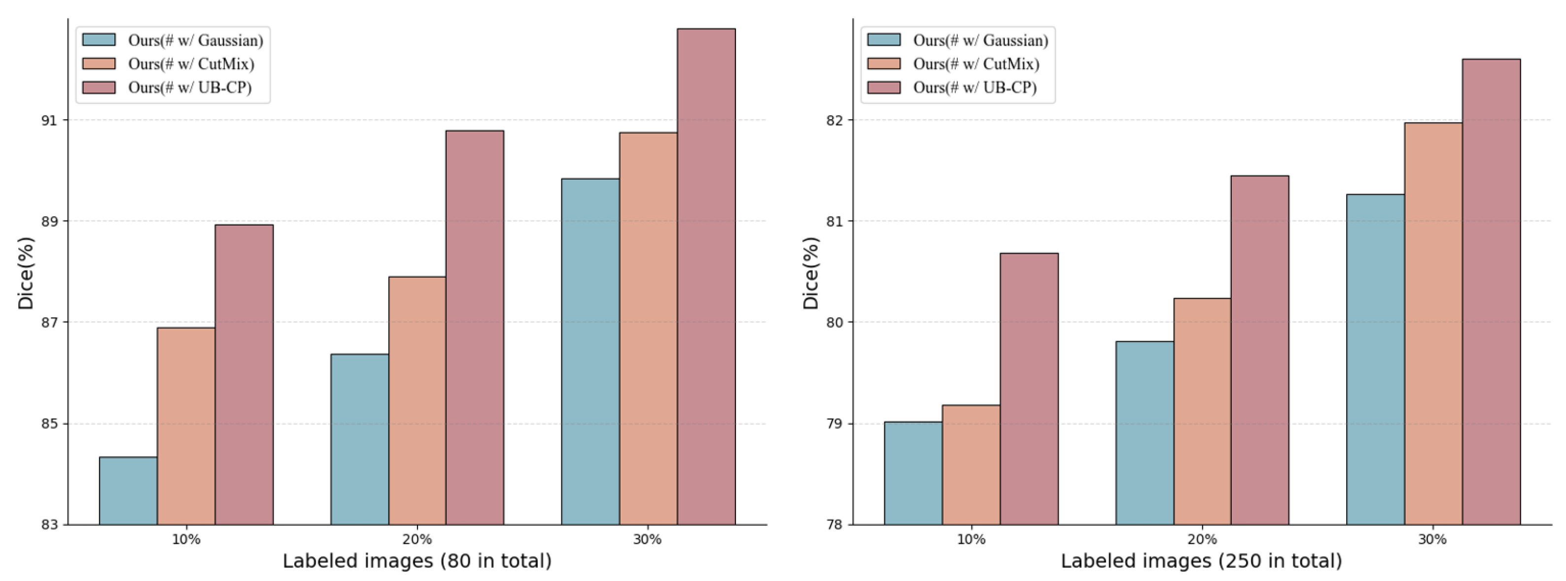
To effectively bridge the potential structural and semantic distribution gap between labeled data $x_u$ and unlabeled data $x_u$, and to mitigate noise interference caused by pseudo-label uncertainty in semi-supervised learning, we propose an uncertainty-guided bidirectional copy–paste (UB−CP) augmentation strategy. The core of this method lies in utilizing the uncertainty estimated via $\mathrm{MC}\mathrm{Dropout}$ during the warm-up phase to dynamically and selectively guide the copy–paste operations.

During the warm-up phase of $f(X,{\theta }^{S1})$, we employ Monte Carlo Dropout on the teacher network to estimate voxel-level uncertainty by computing the mean prediction entropy across multiple stochastic forward passes. Based on this uncertainty map, we precisely paste the regions with the highest uncertainty from the unlabeled data into the labeled data. This uncertainty-guided mechanism ensures that the regularization loss focuses on the “hard” regions where the model requires further learning. For the labeled data, we still follow the principle of BCP and utilize a zero-centered mask $\mathcal{M}$ for the copy–paste operation. During training, we sample one instance from each set to perform the bidirectional copy–paste operation. We copy–paste the labeled data $X_l$ onto the unlabeled data $X_u$. To introduce accurate boundary information from the labeled data and enforce the model to learn boundary features on the unlabeled domain, we adopt the BCP mechanism using a zero-centered mask. To conduct the copy–paste operation between the image pair, we first generate a zero-centered mask ${\mathcal{M}}_1$:

$${\mathcal{M}}_1\in {\{0,1\}}^{W\times H\times L},{\mathcal{M}}_1\left(v\right)\in \{0,1\},$$

(22)

where ${\mathcal{M}}_1$ is the mask where the voxel value indicates whether the voxel originates from the foreground image 0 or the background image 1. The mask ${\mathcal{M}}_1$ is defined based on a zero-value region with size $\beta H\times \beta W\times \beta L$:

$${\mathcal{M}}_1\left(v\right)=\left\{\begin{array}{cc}0\hfill & \mathrm{if}v\in \mathrm{Center}\mathrm{Block}\mathrm{of}\mathrm{size}\beta W\times \beta H\times \beta L\hfill \\ 1\hfill & \mathrm{otherwise}\hfill \end{array}\right.$$

(23)

where $\beta \in (0,1)$. The parameter $\beta$ controls the size ratio of the central block, and the resulting mixed volume $x_{copy}$ is generated by the formula:

$$x_{copy}=x_u\odot {\mathcal{M}}_1+x_l\odot (1-{\mathcal{M}}_1)$$

(24)

This operation pastes the central block of $x_l$ onto the central region of $x_u$. Subsequently, we copy–paste the unlabeled data $x_u$ onto the labeled data $x_l$. This direction aims to transfer the most uncertain unlabeled regions onto the labeled data for proper regularization. We first employ the teacher network $f(X,{\theta }^T)$ combined with Monte Carlo Dropout to estimate the predictive uncertainty. The average prediction probability ${\overline{P}}^t$ is obtained through $N=8$ forward passes:

$${\overline{P}}^t\left(v\right)={\displaystyle \frac{1}{N}}\sum _{n=1}^N{P}_n^t\left(v\right),\forall v\in x_u,$$

(25)

where N is the number of forward passes, and $P_n^t\left(v\right)$ is the prediction probability at voxel v during the n-th pass of the teacher network.

The voxel-level uncertainty is quantified using the average prediction entropy $U\left(v\right)$:

$$U\left(v\right)=-\sum _{c=1}^C{\overline{P}}^t{\left(v\right)}_{c}log\left({\overline{P}}^t{\left(v\right)}_c\right),U\in {\mathbb{R}}^{W\times H\times L},$$

(26)

where C is the number of segmentation classes, and ${\overline{P}}^t{\left(v\right)}_c$ is the average probability for class c at voxel v.

We define the target volume $\mathcal{B}$ for the copied patch as half of the zero-centered region, and the volume of this $\mathcal{B}$ is ${\displaystyle \frac{1}{2}}(\beta W\times \beta H\times \beta L)$. By sliding a window over the uncertainty map U and selecting the two non-overlapping blocks with the highest average uncertainty, ${\mathcal{B}}_1$ and ${\mathcal{B}}_2$, we define the indicator function $\mathcal{B}\left(v\right)$ for the zero-value regions as

$$\mathcal{B}\left(v\right)=\left\{\begin{array}{cc}1\hfill & \mathrm{if}v\in {\mathcal{B}}_1\mathrm{or}v\in {\mathcal{B}}_2\hfill \\ 0\hfill & \mathrm{otherwise}\hfill \end{array}\right..$$

(27)

By combining ${\mathcal{B}}_1$ and ${\mathcal{B}}_2$, we obtain the mask ${\mathcal{M}}_2$, where the values are set to 1 within the $\mathcal{B}$ regions and 0 elsewhere, thus pasting the most uncertain voxel blocks from the unlabeled data onto $x_l$, forming the mixed volume $x_{paste}$:

$$x_{paste}=x_u\odot {\mathcal{M}}_2+x_l\odot (1-{\mathcal{M}}_2)$$

(28)

For the bidirectionally mixed data $x_{\mathrm{copy}}$ and $x_{\mathrm{paste}}$, we feed them into the student network $f(·)$ to obtain the corresponding predictions $p_{\mathrm{copy}}^{S1}$ and $p_{\mathrm{paste}}^{S1}$. To ensure data alignment, the supervision labels for consistency learning on the other student network are also constructed by mixing labeled and unlabeled data. Accordingly, the pseudo-labels for the two branches are defined as

$$\left\{\begin{array}{cc}\hfill {\widehat{y}}_{\mathrm{copy}}^{S2}& ={\widehat{y}}_u^{S2}·{\mathcal{M}}_1+y_l·(1-{\mathcal{M}}_1),\hfill \\ \hfill {\widehat{y}}_{\mathrm{paste}}^{S2}& ={\widehat{y}}_u^{S2}·{\mathcal{M}}_2+y_l·(1-{\mathcal{M}}_2),\hfill \end{array}\right.$$

(29)

where ${\mathcal{M}}_1$ and ${\mathcal{M}}_2$ are the binary masks used for region mixing, ${\widehat{y}}_u^{S2}$ denotes the pseudo-labels generated from unlabeled data, and $y_l$ represents the ground-truth labels from labeled data.

3.4. Fractal-Dimension-Weighted Consistency Regularization

Fractal dimension (FD) serves as a single metric to quantify structural complexity and irregularity, particularly effective for analyzing complex biological structures common in medical images. Regions with higher FD values indicate more intricate structures and irregular textures, often containing richer diagnostic information (e.g., organ boundaries). Standard consistency regularization often overfits simple regions and underperforms in structurally complex areas. 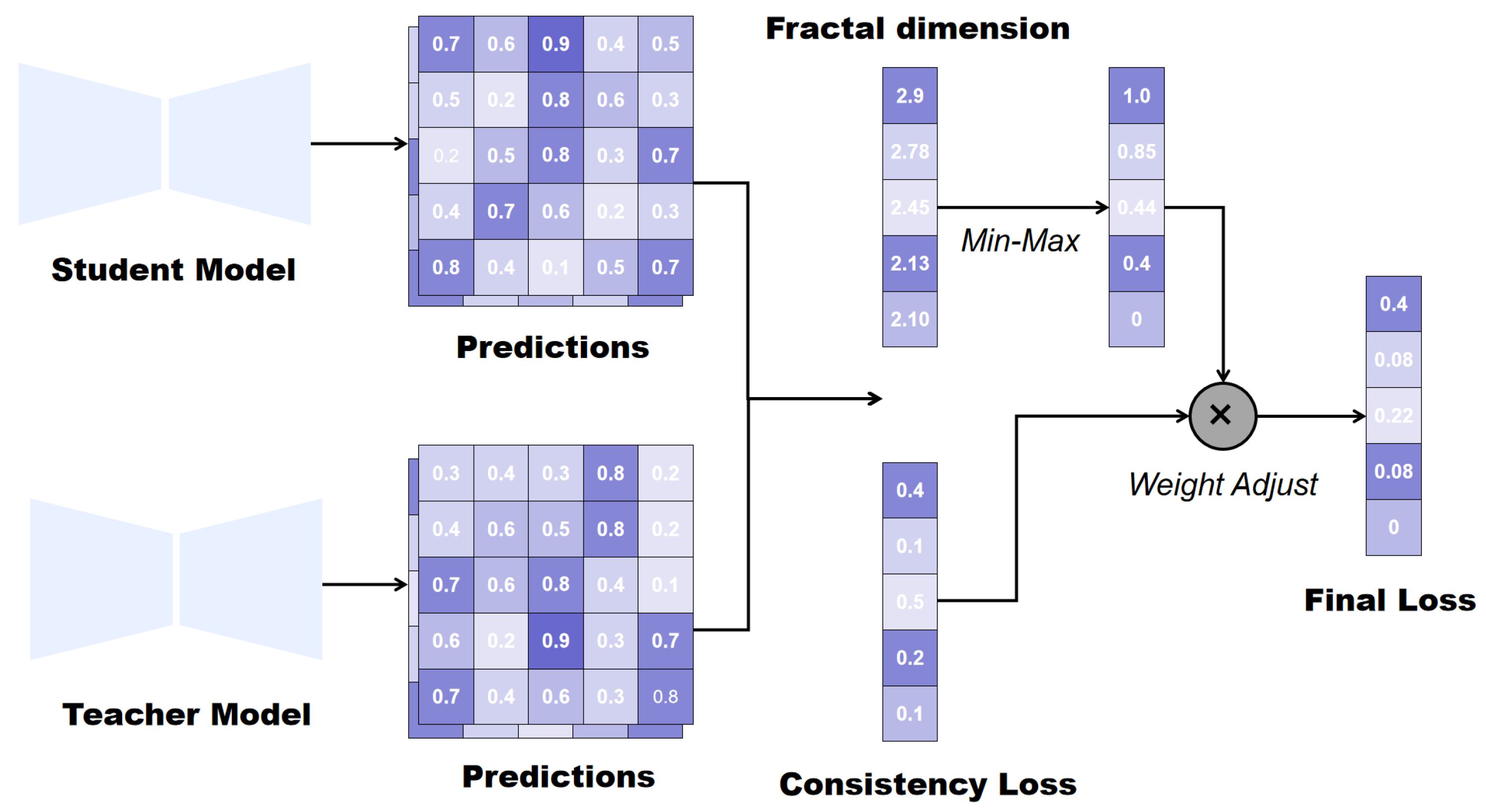We introduce the ${\mathcal{L}}_{\mathrm{fd}}$ to reflect local structural complexity via FD, ensuring stronger supervision signals in challenging regions. Figure 4 illustrates the process of applying fractal dimensions to consistency regularization.

For an input 3D image volume $X\in {\mathbb{R}}^{H\times W\times L}$, we compute the local fractal dimension $\mathrm{FD}\left(v\right)$ for each voxel position $v=(x,y,z)$ using the 3D box-counting method. The $\mathrm{FD}\left(v\right)$ is approximated by

$$\mathrm{FD}\left(v\right)={\displaystyle \frac{\Delta log{N}_r\left(v\right)}{\Delta log(1/r)}},$$

(30)

where r denotes the side length of the box, and $N_r\left(v\right)$ represents the minimum number of boxes with scale r required to cover the non-zero voxels within the local block centered at voxel v. The computation of $N_r\left(v\right)$ follows the differential box-counting strategy described in [40]. Specifically, we set the box scale range to $2\le r\le 7$. The result is a fractal-dimension map that precisely matches the spatial dimensions of the input volume.

The biological structures, such as organs, blood vessels, or tumors, although complex, are not ideal mathematical fractals. They exhibit statistical self-similarity within a finite range of scales, resulting in small differences between the calculated FD values. To increase the model’s discriminative power between different regions, we apply Min-Max normalization to the FD values. The processed weights, ranging from 0 to $1.0$, provide a clear gradient signal for consistency learning between the models:

$$w\left(v\right)={\displaystyle \frac{\mathrm{FD}\left(v\right)-min\left(\mathrm{FD}\right)}{max\left(\mathrm{FD}\right)-min\left(\mathrm{FD}\right)+ϵ}},$$

(31)

where $max\left(\mathrm{FD}\right)$ is the global maximum FD, $min\left(\mathrm{FD}\right)$ is the global minimum FD, and $ϵ$ is a minimal constant.

Assigning higher weights to complex regions forces the student model to focus on aligning its predictions with the teacher model’s distribution in these challenging areas, thereby enhancing consistency along boundaries and complex structural regions. Areas with high FD values are typically critical decision regions in semantic segmentation, yet also the most error-prone. Building upon this weighted learning mechanism, we further incorporate uncertainty estimation by performing alignment only on voxels whose uncertainty falls below a predefined threshold. This approach assigns higher weights to complex regions while preserving numerical smoothness and avoiding excessive bias. The weighted consistency regularization term ${\mathcal{L}}_{\mathrm{fd}}$ is defined as

$${\mathcal{L}}_{\mathrm{fd}}={\displaystyle \frac{1}{N}}\sum _{v}w\left(v\right)·D_{\mathrm{KL}}\left(p^T\left(v\right),p^S\left(v\right)\right)·\mathbb{I}(U\left(v\right)<\psi \left(U\right)),$$

(32)

where $\mathbb{I}(·)$ is the indicator function, and the constraint $\mathbb{I}\left(U\right(v)<\psi (U\left)\right)$ ensures that the loss is only calculated for voxels v where the uncertainty $U\left(v\right)$ is below the threshold $\psi \left(U\right)$. N is the total number of voxels, and $p^T\left(v\right)$ and $p^S\left(v\right)$ are the prediction probability distributions of the teacher and student networks, respectively.

To enable the model to learn more complex knowledge without being overly affected by noise, we empirically set an uncertainty threshold, where $\psi (·)$ computes the top $30\%$ quantile value. The Kullback–Leibler (KL) divergence $D_{\mathrm{KL}}$ is given by

$$D_{\mathrm{KL}}\left(p^T\left(v\right),p^S\left(v\right)\right)=p^T\left(v\right)log{\displaystyle \frac{p^T\left(v\right)+ϵ}{p^S\left(v\right)+ϵ}},$$

(33)

where $ϵ$ is a minimal constant set to ${10}^{-8}$, introduced to maintain numerical stability.

4. Loss Function

Our model’s objective is achieved by optimizing a comprehensive loss function that combines both supervised ${\mathcal{L}}_{\sup }$ and unsupervised ${\mathcal{L}}_{\mathrm{unsup}}$ components. We first define the supervised loss and then present the total objective function. The supervised loss guides the student networks’ training on the limited set of labeled data by comparing their predictions against the ground truth. Following standard practice in medical segmentation, the supervised loss for each student network is a combination of the cross-entropy loss and the Dice loss. For student network $f(X,{\theta }^{S1})$, the supervised loss on the labeled data $D_l$ is defined as

$${\mathcal{L}}_{\sup 1}({\mathbf{p}}_l^{S1},{\mathbf{y}}_l)={\mathcal{L}}_{\mathrm{ce}}({\mathbf{p}}_l^{S1},{\mathbf{y}}_l)+{\mathcal{L}}_{\mathrm{Dice}}({\mathbf{p}}_l^{S1},{\mathbf{y}}_l),$$

(34)

where $p_l^{S1}$ is the prediction result of $S1$ for the labeled input, and $y_l$ is the corresponding ground-truth label. The CE loss ensures pixel-wise classification accuracy, while the Dice loss addresses potential class imbalance and focuses on optimizing the region overlap.

The supervised loss ${\mathcal{L}}_{\sup 2}$ for the second student network $f(X,{\theta }^{S2})$ is computed identically. The total supervised loss ${\mathcal{L}}_{\sup }$ is the sum of the individual losses from the two student networks, ensuring both models are anchored to the available ground truth:

$${\mathcal{L}}_{\sup }={\mathcal{L}}_{\sup 1}+{\mathcal{L}}_{\sup 2}.$$

(35)

The overall objective function is a weighted combination of the total supervised loss ${\mathcal{L}}_{\sup }$ and the overall unsupervised loss ${\mathcal{L}}_{\mathrm{unsup}}$, enabling effective knowledge transfer from the large amount of unlabeled data. The overall loss (${\mathcal{L}}_{\mathrm{total}}$) is calculated as

$${\mathcal{L}}_{\mathrm{total}}={\mathcal{L}}_{\sup }+\sigma ·{\mathcal{L}}_{\mathrm{unsup}},$$

(36)

where $\sigma$ is a scalar coefficient that dynamically weights the contribution of the unsupervised terms during training. The unsupervised loss ${\mathcal{L}}_{\mathrm{unsup}}$ is composed of three distinct mechanisms designed to enhance feature consistency, leverage pseudo-supervision, and enforce structural integrity:

$${\mathcal{L}}_{\mathrm{unsup}}={\mathcal{L}}_{\mathrm{cl}}+{\mathcal{L}}_{\mathrm{cps}}+{\mathcal{L}}_{\mathrm{fd}},$$

(37)

The ${\mathcal{L}}_{\mathrm{cl}}$ is the hierarchical contrastive loss, ${\mathcal{L}}_{\mathrm{cps}}$ is the cross-pseudo-supervision loss, and ${\mathcal{L}}_{\mathrm{fd}}$ is the fractal-dimension-weighted consistency loss. The specific calculation methods for these unsupervised loss components have been detailed in the preceding sections.

5. Experiments

5.1. Dataset

The LA dataset [47], derived from the 2019 Atrial Segmentation Challenge, contains 100 3D gadolinium-enhanced MRI scans along with corresponding expert annotations. Among these, 80 isotropic scans are used for training and 20 for testing. To evaluate our method in a semi-supervised learning setting, we randomly select 20% of the training samples as labeled data, while the remaining 80% are treated as unlabeled data. For a fair comparison, we follow the same preprocessing strategy as previous works [19], which includes cropping each image to a 3D subvolume of size 112 × 112 × 80, focusing on the heart region and applying intensity normalization. We compare our approach against other methods under 20% and 10% labeled data settings.

The BraTS2019 dataset [48], collected as part of the Brain Tumor Segmentation Challenge, consists of 335 samples with a resolution of 240 × 240 × 155 mm³;. Each sample includes four types of brain MRI scans: T1-weighted, T1-weighted with contrast enhancement, T2-weighted, and T2-FLAIR. Following previous studies [17], we use T2-FLAIR scans for our experiments. Each sample underwent center cropping and was resampled to an isotropic resolution of $1.0\times 1.0\times 1.0{\mathrm{mm}}^3$. In our experiments, 250 scans were used for training, 25 for validation, and 60 for testing. Similar to the LA dataset, we evaluated the performance of our method against others under $20\%$ and $10\%$ labeled data conditions.

5.2. Implementation Details

Our experiments were implemented using the PyTorch framework. The experimental hardware configuration included an NVIDIA RTX 3090 GPU and an Intel Xeon Gold 6330 processor equipped with 14 virtual CPUs (vCPUs). We adopted an improved Mean Teacher model as the baseline and introduced an auxiliary student model on top of it. Following prior work, we ran 6000 iterations on the LA dataset and 20,000 iterations on the BraTS 2019 dataset. All methods were optimized using the SGD optimizer with momentum set to 0.9 and weight decay set to 0.0001. The total batch size was set to 4, with each batch containing 2 labeled images and 2 unlabeled images. The initial learning rate was 0.01, reduced by 0.1 every 2500 iterations. Parameter ${\lambda }_t$ was set to 1, while ${\lambda }_h$ and ${\lambda }_l$ employed time-dependent Gaussian warm-up functions to stabilize the training process. The code was implemented using PyTorch (https://pytorch.org/), and all experiments utilized a fixed random seed of 1337 to ensure reproducibility.

5.3. Evaluation Metrics

To comprehensively evaluate model performance in medical image segmentation tasks, this study employs four widely adopted metrics: Dice Coefficient, Jaccard Index, 95% Hausdorff Distance, Average Surface Distance.

The Dice Coefficient quantifies the spatial overlap between predicted and ground-truth segmentations. It is formally defined as twice the intersection area divided by the sum of prediction and ground-truth areas:

$$Dice={\displaystyle \frac{2|P\cap G|}{\left|P\right|+\left|G\right|}}$$

(38)

where P represents the predicted segmentation region, G represents the ground-truth segmentation region, and $|·|$ denotes the number of voxels in a set. The Jaccard Index (also known as Intersection over Union, IoU) measures the ratio between the intersection and the union of the predicted and ground-truth regions and is defined as

$$Jaccard={\displaystyle \frac{|P\cap G|}{|P\cup G|}}$$

(39)

The Hausdorff Distance is used to measure the maximum of the minimum distances between two sets of boundary points. The 95% Hausdorff Distance (95HD) takes the 95th percentile of all the point-to-set distances to reduce the influence of outliers. Let d(x,G) denote the minimum distance from point x to set G, then the 95HD is defined as

$$95HD(P,G)=max\left\{\underset{x\in P}{{\mathrm{p}}_{95}}\left(d(x,G)\right),\underset{y\in G}{{\mathrm{p}}_{95}}\left(d(y,P)\right)\right\}$$

(40)

where ${\mathrm{p}}_{95}$ denotes the 95th percentile operation. The Average Surface Distance (ASD) measures the mean minimum distance between predicted and ground truth boundaries, defined as

$$ASD(P,G)={\displaystyle \frac{1}{\left|P\right|+\left|G\right|}}\left(\sum _{x\in P}d(x,G)+\sum _{y\in G}d(y,P)\right)$$

(41)

The Average Surface Distance (ASD) provides an averaged measure of the overall discrepancy between two boundary point sets, serving to quantify the global accuracy of model segmentation results.

5.4. Experiments on the LA Dataset

In

Table 2. Comparison with state-of-the-art methods on the LA dataset. The * denotes $p<0.05$, and ** denotes $p\le 0.01$ in paired t-tests.

Method	Labeled/Unlabeled	Dice (%) ↑	Jaccard (%) ↑	95HD (voxel) ↓	ASD (voxel) ↓
V-Net	8 (10%)/0	77.87 ± 8.12	66.56 ± 10.81	18.77 ± 13.42	21.25 ± 3.18
V-Net	16 (20%)/0	85.68 ± 8.26	75.58 ± 6.31	14.65 ± 5.74	14.48 ± 2.71
CPS [21]	8 (10%)/72 (90%)	84.89 ± 5.63	74.63 ± 8.92	18.56 ± 11.43	3.82 ± 2.35
UA-MT [17]		85.55 ± 6.41 *	76.45 ± 9.84 *	15.68 ± 12.27	2.78 ± 3.32
BCP [29]		87.91 ± 4.88 *	78.72 ± 7.41 *	10.90 ± 15.12 *	2.88 ± 4.84
DTC [19]		87.26 ± 7.17 *	77.12 ± 9.66 *	8.15 ± 12.58	2.61 ± 2.96
UPRC [18]		87.46 ± 4.95 **	77.65 ± 7.88 **	9.45 ± 13.92	2.85 ± 3.74 *
SLC-Net [49]		86.77 ± 7.52	78.15 ± 10.11	9.83 ± 11.65	2.56 ± 2.47
MC-Net [24]		88.24 ± 4.36	79.19 ± 6.83	7.85 ± 10.32 *	1.95 ± 2.08
Contrimix [50]		87.45 ± 6.92 **	77.61 ± 8.41 **	10.24 ± 12.63 *	2.39 ± 3.24
DSMT-Net [51]		87.85 ± 6.24	78.54 ± 7.83	8.25 ± 10.93	2.21 ± 2.31
Ours		88.92 ± 5.58	79.85 ± 7.82	8.04 ± 12.64	1.84 ± 2.71
CPS [21]	16 (20%)/64 (80%)	86.87 ± 3.66	78.67 ± 6.82	12.87 ± 3.44	2.35 ± 1.52
UA-MT [17]		87.23 ± 2.85 **	79.77 ± 4.22 **	7.45 ± 3.21	1.69 ± 1.41
BCP [29]		90.12 ± 5.88 **	81.47 ± 10.94 **	9.27 ± 4.68 **	2.26 ± 1.86
DTC [19]		89.45 ± 4.79 *	80.56 ± 7.21 *	7.27 ± 5.86	1.92 ± 2.04
UPRC [18]		88.24 ± 1.88 *	79.27 ± 3.76 *	8.49 ± 2.12 *	2.07 ± 0.96
SLC-Net [49]		88.79 ± 3.27	80.15 ± 5.66	8.46 ± 3.24	1.82 ± 1.65
MC-Net [24]		90.42 ± 2.91 *	82.06 ± 4.38 *	6.65 ± 3.45	1.99 ± 1.74 *
Contrimix [50]		90.23 ± 2.74 **	81.73 ± 5.43 **	7.15 ± 3.56 *	2.39 ± 1.62
DSMT-Net [51]		89.49 ± 2.49	80.73 ± 5.44	6.87 ± 4.06	1.63 ± 1.83
Ours		90.78 ± 2.64	82.72 ± 5.38	6.07 ± 2.74	1.57 ± 1.29

, we report the comparative results on the LA dataset using both 10% and 20% labeled data for our method and several state-of-the-art semi-supervised segmentation approaches.

On the LA dataset, we first evaluate the fully supervised V-Net using 10% and 20% labeled data. As expected, increasing the number of labeled scans from 8 to 16 leads to a substantial performance gain, with Dice improving from 77.87% to 85.68% and Jaccard increasing from 66.56% to 75.58%. However, similar to our observations on BraTS 2019, supervised learning remains limited when annotations are scarce, particularly in boundary-focused metrics such as 95HD and ASD. Under the 10% labeled setting, incorporating the large amount of unlabeled scans substantially boosts segmentation accuracy across most semi-supervised approaches. Methods such as UA-MT, BCP, DTC, UPRC, and Contrimix achieve statistically significant improvements in Dice and Jaccard, demonstrating the benefits of leveraging unlabeled information. MC-Net and DSMT-Net exhibit particularly strong performance, especially in reducing boundary errors. Our method achieves a Dice of 88.92% and a Jaccard of 79.85%, together with a low ASD of 1.84, indicating more accurate region segmentation and smoother anatomical boundaries than most competing approaches.

When the labeled ratio increases to 20%, all methods continue to improve, but the performance gap between state-of-the-art approaches becomes more evident. Approaches such as UA-MT, BCP, DTC, MC-Net, and Contrimix report highly significant gains ($p<0.05$ or $p\le 0.01$), showing their effectiveness at higher annotation budgets. Nevertheless, our method consistently achieves the best overall results, reaching 90.78% Dice and 82.72% Jaccard, while also obtaining the lowest 95HD (6.07) and ASD (1.57). These improvements indicate that our framework not only enhances volumetric accuracy but also yields more stable and anatomically coherent boundaries. Overall, across both low-label and medium-label settings, our method demonstrates strong robustness and outperforms the fully supervised baseline as well as the majority of existing semi-supervised segmentation models. The consistent improvements across all evaluation metrics validate the effectiveness of our approach on the LA dataset.

As shown in Figure 5, under the 20% labeled data condition, we present segmentation results on the LA dataset comparing our method to several alternatives. Clearly, in some hard-to-discriminate regions (e.g., blurred boundaries or complex structures), our approach shows stronger robustness.

To further highlight our method’s performance advantage, we also plotted line charts of Dice and Jaccard metrics across different label ratios, as shown in Figure 6.

The results demonstrate that our method gains substantially over the purely supervised model V-Net, especially when labeled samples are extremely scarce, and outperforms other models on both segmentation metrics Dice and Jaccard.

5.5. Experiments on the BraTS 2019 Dataset

We conducted extensive comparative experiments on the BraTS 2019 dataset to validate the effectiveness and robustness of our proposed method in the task of brain tumor segmentation, as shown in

Table 3. Comparison experiments on BraTS 2019. The * denotes $p<0.05$, and ** denotes $p\le 0.01$ in paired t-tests.

Method	Scans Used	Metrics
	Labeled Unlabeled	Dice (%) ↑	Jaccard (%) ↑	95HD (voxel) ↓	ASD (voxel) ↓
V-Net	25 (10%)/0	66.23 ± 12.84	58.81 ± 15.27	14.69 ± 16.83	4.46 ± 4.12
V-Net	50 (20%)/0	71.61 ± 10.15	63.46 ± 13.68	11.05 ± 14.27	3.97 ± 3.65
CPS [21]	25 (10%)/225 (90%)	76.87 * ± 10.92	66.46 * ± 14.31	11.45 ± 19.74	3.11 ± 4.88
UA-MT [17]		78.86 ± 10.47	68.26 ± 13.89	9.12 ± 14.33	2.46 ± 3.67
DTC [19]		78.35 * ± 10.68	67.89 * ± 13.95	12.37 ± 16.12	3.64 ± 4.31
UPRC [18]		77.78 ± 11.14	67.24 ± 14.58	11.12 * ± 15.46	2.35 ± 3.72
SLC-Net [49]		80.13 * ± 9.87	69.24 * ± 13.42	9.43 ± 13.88	2.56 ± 3.45
BCP [29]		79.84 ± 14.33	68.73 ± 17.01	9.53 ± 14.27	2.25 ± 3.91
MC-Net [24]		80.12 * ± 9.94	69.11 * ± 13.67	10.68 ± 14.37	2.98 ± 3.18
Contrimix [50]		79.93 ± 11.47	68.46 ± 14.86	11.68 ± 14.86	2.98 ± 3.72
DSMT-Net [51]		78.46 * ± 12.29	67.57 * ± 13.67	9.23 ± 10.59	2.98 ± 3.88
Ours		80.68 ± 8.12	69.48 ± 11.23	8.64 ± 12.47	2.47 ± 2.68
CPS [21]	50 (20%)/200 (80%)	79.06 * ± 9.33	68.86 * ± 12.78	9.14 ± 20.66	2.07 ± 5.14
UA-MT [17]		80.36 * ± 8.87	69.75 * ± 12.33	8.79 ± 10.93	1.95 * ± 2.83
DTC [19]		78.96 ± 10.76	67.96 ± 14.11	9.41 * ± 15.08	2.81 ± 3.67
UPRC [18]		79.35 ** ± 8.58	70.29 * ± 11.02	7.74 ± 9.67	2.14 ± 2.84
SLC-Net [49]		80.93 * ± 8.71	69.49 * ± 12.19	8.46 * ± 11.84	2.46 ± 3.11
BCP [29]		80.67 * ± 7.02	70.11 * ± 9.86	9.04 ± 17.83	2.37 ± 4.28
MC-Net [24]		81.28 ± 6.56	70.24 ± 9.28	9.47 * ± 12.41	2.69 ± 3.03
Contrimix [50]		81.23 * ± 8.17	70.05 * ± 12.34	9.54 ± 6.82	2.98 ± 2.48
DSMT-Net [51]		78.86 ± 7.87	67.84 ± 10.82	8.68 * ± 14.35	1.91 ± 3.36
Ours		81.45 ± 7.38	71.18 ± 10.67	7.98 ± 9.94	1.88 ± 2.71

. We compare our performance against a series of state-of-the-art semi-supervised segmentation approaches under both the $10\%$ and $20\%$ labeled data proportions. Similarly, we present the comparison of segmentation results for different methods under the $20\%$ labeled data proportion in Figure 7.

In the BraTS 2019 dataset, we first evaluate the fully supervised baseline V-Net under limited annotations. When increasing the labeled scans from 10% (25 scans) to 20% (50 scans), the Dice score improves from 66.23% to 71.61% and the Jaccard index increases from 58.81% to 63.46%, demonstrating the strong dependence of supervised learning on annotation quantity. However, compared with the semi-supervised approaches, the performance of V-Net remains clearly inferior.

Under the 10% labeled/90% unlabeled setting, most semi-supervised methods (e.g., CPS, DTC, SLC-Net, MC-Net, and DSMT-Net) outperform the supervised baseline in both Dice and Jaccard, indicating that leveraging abundant unlabeled data greatly benefits tumor segmentation. Methods such as SLC-Net and MC-Net achieve statistically significant improvements ($p<0.05$), although their boundary-related metrics (95HD and ASD) still show relatively large variance. In contrast, our method achieves 80.68% Dice and 69.48% Jaccard, while also producing lower 95HD (8.64) and ASD (2.47), suggesting that it provides more accurate region segmentation and more stable boundary localization.

When increasing the annotation ratio to 20% labeled/80% unlabeled, the performance of all methods improves further, but the differences between approaches become more pronounced. Classical semi-supervised methods such as UPRC, SLC-Net, BCP, and MC-Net show significant or highly significant gains. Nevertheless, our approach still achieves the best overall performance, reaching 81.45% Dice and 71.18% Jaccard (Figure 8), while also offering competitive or superior results in 95HD and ASD. This demonstrates the robustness and generalization ability of our framework across different annotation budgets.

Overall, across both annotation settings, our method consistently surpasses the fully supervised baseline and most existing semi-supervised segmentation methods. The improvements in both region-based and boundary-based metrics validate the effectiveness of our approach in exploiting unlabeled data and enhancing tumor segmentation quality on BraTS 2019.

5.6. Effect of the Uncertainty Threshold $\psi (·)$

In the hierarchical contrastive learning mechanism, we partition the high and low confidence sets based on an uncertainty threshold. To evaluate the influence of this confidence threshold, we conduct experiments using different settings for the uncertainty threshold $\psi (·)$ to explore its impact on model performance; we conducted an ablation study on the BraTS 2019 dataset with a 10% labeled data ratio, and the results are shown in

Table 4. Ablation study of the uncertainty threshold $\psi (·)$.

$\mathit{\psi }(·)$	Dice (%) ↑	Jaccard (%) ↑	95HD (voxel) ↓	ASD (voxel) ↓
$5\%$	79.55	68.32	11.34	2.98
$10\%$	80.26	69.04	10.52	2.43
$20\%$	80.49	69.21	10.24	2.68
$30\%$	80.68	69.48	9.84	2.27
$40\%$	80.24	69.16	10.48	2.75

. This threshold is used to filter high-confidence pseudo-labels, guiding the network to perform consistency learning.

Experimental results indicate that as the uncertainty threshold $\psi (·)$ increases, the segmentation performance of the model exhibits a trend of first rising and then declining. Specifically, as the threshold gradually increases from $5\%$ to $30\%$, the Dice score steadily improves from $79.55\%$ to a peak of $80.68\%$; simultaneously, metrics such as Jaccard, $95\mathrm{HD}$, and ASD also achieve optimal performance. This confirms that applying consistency constraints to more high-confidence voxels under moderately relaxed conditions enables the network to learn richer and more accurate feature information, thereby effectively enhancing segmentation performance. When the threshold is further increased to $40\%$, the Dice score drops to $80.24\%$ and all performance metrics deteriorate. This indicates that an overly lenient threshold causes the network to incorporate more voxels containing uncertainty or erroneous information into its consistency learning objectives. These inaccurate pseudo-labels disrupt model training, negating the positive effects of semi-supervised learning and ultimately limiting further improvements in segmentation performance. Therefore, we set the optimal value of $\psi (·)$ to $30\%$.

5.7. Performance Comparison with Other Strong Data Augmentation Methods

To verify the superiority of our proposed uncertainty-aware bidirectional copy–paste (UB-CP) strategy, we conducted comparative experiments against two commonly used strong data augmentation methods, namely Gaussian Noise only and CutMix, on the BRATS 2019 and LA datasets, respectively. The experimental results are shown in Figure 9. Our analysis focuses on three different labeled data proportions: $10\%$, $20\%$, and $30\%$. We observe that the effectiveness of all augmentation methods increases as the proportion of labeled data grows.

The performance gain of UB-CP compared to other methods is most evident at the most data-scarce proportion of $10\%$. This indicates that UB-CP can effectively utilize the structural information within the unlabeled data to generate high-quality pseudo-labels and augmented samples, thereby providing stronger regularization and generalization capability to the model when the data volume is limited.

On the LA dataset (left figure), the UB-CP method achieves a Dice score close to $90\%$, which is significantly higher than the performance of CutMix and Gaussian Noise. On the BRATS 2019 dataset (right figure), when the labeled data reaches $30\%$, the UB-CP model’s Dice score exceeds $82.5\%$, while the other two methods remain below $82\%$. This further demonstrates the strong capability of UB-CP in enriching the diversity of training samples.

5.8. Effect of the Uncertainty-Aware Bidirectional Copy–Paste Parameters

We further conducted an ablation study to evaluate the influence of two key hyperparameters in our proposed uncertainty-aware bidirectional copy–paste strategy: the number of mask blocks n and the volume ratio $\beta$ on the segmentation performance on the LA dataset with $10\%$ and $20\%$ labeled data. The parameter n controls the number of independent mask blocks utilized for copy–paste, while $\beta$ determines the ratio of the overall cut volume to the original image volume. The experimental results are presented in

Table 5. Metrics for different n and $\beta$ values.

Labeled	Unlabeled	n	$\mathit{\beta }$	Dice ↑	Jaccard ↑	95HD ↓	ASD ↓
16 (20%)	84 (80%)	2	1/2	89.82	81.17	9.14	2.43
			2/3	90.46	82.45	6.54	1.79
			3/4	90.78	82.72	6.07	1.57
			4/5	90.35	82.34	7.12	1.93
		3	1/2	88.32	80.97	9.68	2.70
			2/3	88.64	82.34	6.89	1.73
			3/4	88.57	82.15	6.34	1.84
			4/5	89.26	81.91	6.38	2.08
8 (10%)	72 (90%)	2	1/2	87.50	75.68	9.46	2.52
			2/3	88.76	79.57	7.71	1.72
			3/4	88.92	79.85	8.04	1.84
			4/5	88.49	79.96	7.63	2.12
		3	1/2	86.48	77.97	10.50	2.87
			2/3	87.67	78.43	7.60	1.90
			3/4	88.46	79.13	8.34	2.34
			4/5	88.54	79.35	7.44	2.43

.

We observe that the model’s performance is generally superior when $n=2$ compared to the $n=3$ setting. This suggests that dividing the cut volume into $n=2$ mask blocks, each with a volume of $(\beta W\times \beta H\times \beta L)/2$, allows the generated augmented samples to maintain sufficient semantic relevance while effectively introducing cross-voxel perturbations, thereby enhancing the model’s generalization ability. Conversely, setting $n=3$ might lead to mask blocks that are too small or semantically fragmented, slightly compromising the performance.

Building on the $n=2$ setting, the model shows sensitivity to the volume ratio $\beta$. When $\beta$ gradually increases from $1/2$ to $3/4$, the Dice score steadily improves from $89.82\%$ to its peak value of $90.78\%$. Simultaneously, Jaccard, $95\mathrm{HD}$, and ASD metrics also reach their optimal values. This indicates that a moderate increase in the cutting volume $\beta =3/4$ provides richer contextual information and stronger structural consistency constraints. However, when $\beta$ is further increased to $4/5$, the performance slightly decreases. This deterioration may be attributed to the excessively large cutting volume introducing too much noise or disrupting some critical semantic structures. In summary, we select the parameter combination that yields the best performance across all settings, namely $n=2$ for the number of mask blocks and $\beta =3/4$ for the volume ratio, for all main experiments in this study.

5.9. Ablation Study

To evaluate the independent contribution of each module to the overall performance, we conducted a comprehensive ablation study on the LA dataset. Following the standard semi-supervised setting, the experiment uses 16 labeled scans (20%) and 64 unlabeled scans. All quantitative results are summarized in

Table 6. Ablation study of individual components on the LA dataset.

Scans Used		Modules Used				Metrics
Labeled	Unlabeled	I-EMA	${\mathcal{L}}_{\mathbf{cps}}$	${\mathcal{L}}_{\mathbf{hcl}}$	${\mathcal{L}}_{\mathbf{fd}}$	Dice (%) ↑	Jaccard (%) ↑
16	64	✓	✓			87.35	77.82
16	64	✓	✓	✓		90.54	82.46
16	64	✓	✓		✓	87.22	77.51
16	64	✓		✓	✓	89.65	81.45
16	64		✓	✓	✓	90.62	82.50
16	64	✓	✓	✓	✓	90.78	82.72

. For fair comparison and to ensure the basic operability of the framework, we adopt the standard EMA when the I-EMA module is removed and employ the KL divergence for consistency computation when the ${\mathcal{L}}_{fd}$ term is excluded. We first take the configuration containing I-EMA and the consistency loss ${\mathcal{L}}_{cps}$ as the baseline model, which achieves 87.35% Dice and 77.82% Jaccard. After incorporating the hierarchical contrastive loss ${\mathcal{L}}_{hcl}$, the performance improves significantly to 90.54% Dice and 82.46% Jaccard, indicating that the hierarchical contrastive constraints effectively enhance feature discrimination and cross-view consistency. This suggests that fractal-dimension weighting helps the network better capture anatomical boundary details. We also observe that removing the I-EMA module leads to a noticeable decrease in segmentation accuracy. Finally, when all modules—namely I-EMA, ${\mathcal{L}}_{cps}$, ${\mathcal{L}}_{hcl}$, and ${\mathcal{L}}_{fd}$—are jointly optimized, the model achieves the best overall performance, reaching 90.78% in Dice and 82.72% in Jaccard. This result clearly demonstrates that each module contributes critically to the overall performance improvement, and their synergistic combination maximizes the model’s stability and segmentation accuracy.

6. Discussion

Despite the superior performance of the proposed framework compared with existing semi-supervised segmentation methods, several practical considerations remain. Introducing the dual-student architecture, MC-dropout-based uncertainty estimation, and FD graph computation increases the training time computational cost. However, these components are enabled only during training and therefore do not affect inference efficiency. The teacher network incurs the same forward-pass cost as a standard Mean Teacher (MT) framework, and neither uncertainty estimation nor FD computation is required at deployment. Thus, the inference complexity remains comparable to conventional 3D CNN segmentation models. Each additional module is designed to address specific limitations of the MT framework. The dual-student design enhances representation diversity and mitigates confirmation bias, while the I-EMA strategy prevents the teacher from collapsing toward redundant representations. MC dropout improves pseudo-label reliability, and FD weighting assigns greater importance to structurally complex regions. Ablation studies show that removing any module causes notable performance degradation, indicating that the increased training cost is justified by improved accuracy and robustness. Nonetheless, the generalization ability of the framework can still be improved. Because FD weighting and uncertainty estimation rely on image-dependent statistics, large distribution shifts (e.g., scanning protocol differences, magnetic field variation, or strong noise) may reduce their reliability and degrade pseudo-label quality. Likewise, although dual students increase diversity, both may drift similarly when facing substantial domain shifts, reducing the effectiveness of I-EMA. Future work may explore improving cross-domain and cross-device generalization: (1) integrating domain adaptation or domain generalization to stabilize FD estimation and uncertainty prediction under distribution shifts; (2) incorporating pretrained knowledge from foundation models to enhance robustness to rare anatomical patterns or low-quality images; and (3) leveraging synthetic data or generative models to introduce broader structural and imaging variations during training. From the clinical integration perspective, the proposed framework introduces no additional inference-time operations and can be seamlessly integrated into PACS or routine radiology workflows. FD graphs can be precomputed in preprocessing, and UB-CP is also training-only. Therefore, real-world runtime overhead is nearly identical to existing deep-learning segmentation systems. Improved boundary accuracy and robustness may also reduce manual correction effort, suggesting potential clinical value.

7. Conclusions

In this work, we address key challenges in weak-label or semi-supervised segmentation settings—including model coupling, error accumulation, and limited discriminative capacity of representations. Specifically, we propose a novel semi-supervised framework. We design a dual-student architecture in which two student models are respectively subjected to weak and strong perturbations, and incorporate an independence-aware exponential moving average (I-EMA) update mechanism to effectively alleviate the network-dependency issue inherent in the traditional Mean-Teacher paradigm. We further introduce an uncertainty-aware bidirectional copy–paste (UB-CP) data augmentation method to enhance sample diversity while avoiding excessive perturbation. Meanwhile, we embed a hierarchical contrastive learning (HCL) mechanism that enforces feature consistency at global, high-confidence, and low-confidence levels, and guide the consistency loss between teacher and student networks with fractal-dimension (FD) weighting, thereby boosting the discriminative power of the feature space. Mechanistically, the I-EMA module dynamically adjusts the update speed of the teacher network—slowing down when network dependency is high, and accelerating when it is low—thereby improving training stability; the UB-CP augmentation preserves structural-semantic consistency while introducing rich sample perturbations, enhancing the model’s robustness; the HCL module, by constructing contrastive objectives across multiple confidence levels and scales, significantly strengthens feature separability and improves boundary delineation and pseudo-label quality. To validate our method, we conduct large-scale experiments on two public datasets, BraTS 2019 and LA, under $10\%$ and $20\%$ labeled data ratios. The results clearly demonstrate the superior performance of our approach across all settings: On the LA dataset, with $10\%$ labeled data, our model achieves a Dice score of $88.92\%$ and an ASD of $1.84$ voxels. With $20\%$ labeled data, we achieve the best performance, recording a Dice score of $90.78\%$ and a $95\mathrm{HD}$ of $6.07$ voxels. On the BraTS 2019 dataset, with $10\%$ labeled data, we achieve a Dice score of $80.68\%$ and a $95\mathrm{HD}$ of $8.64$ voxels. With $20\%$ labeled data, the Dice score reaches $81.45\%$ and the ASD is $1.88$ voxels. These comprehensive results not only significantly outperform current state-of-the-art semi-supervised methods but also demonstrate our method’s potential to successfully exploit unlabeled data and enhance model generalization under extremely sparse annotation conditions.