Dynamical Analysis of Time Fractional Radial Groundwater Flow Equation

Abstract

In this study, a time-fractional extension of the classical Theis problem with an exponential source term is investigated in a confined aquifer. The governing equation is modeled using two different fractional derivatives—the Caputo and Atangana–Baleanu–Caputo (ABC) operators—to account for memory effects in groundwater flow. The Fractional Reduced Differential Transform Method (FRDTM) is applied to obtain approximate series solutions up to the fifth order. The impact of the fractional order $\alpha$, the nature of the fractional kernel and the localized source term on the hydraulic head are explored at different radial positions. The comparative analysis between the Caputo and Atangana–Baleanu–Caputo (ABC) models reveals how memory effects and operator choice significantly influence the hydraulic head response, offering insights into selecting suitable models for aquifers with varying recharge characteristics.

1. Introduction

Groundwater hydrology plays a critical role in sustaining water supplies for agricultural, industrial and domestic use worldwide [1,2,3]. It involves the study of subsurface water movement through porous geological formations and its interaction with surface water bodies [4]. Understanding groundwater flow dynamics is essential for effective water resource management, contamination assessment and environmental protection [5]. The complexity of aquifer systems—owing to heterogeneity, anisotropy, and external drivers such as recharge and pumping—necessitates robust mathematical models to accurately predict groundwater behavior [6].

The classical groundwater flow model, derived by combining Darcy’s law with the principle of mass conservation, provides a foundational partial differential equation (PDE) that governs the transient flow of groundwater through confined aquifers [7]. These models typically describe the hydraulic head distribution and its temporal evolution under various boundary and initial conditions. Analytical and numerical solution techniques, including finite difference methods [3,8,9,10,11], finite element methods [12,13,14,15] and integral transform methods, have been extensively employed to solve these PDEs. However, classical models based on integer-order derivatives sometimes fail to capture the complex, memory dependent processes observed in real aquifer systems, such as anomalous diffusion or long-range interactions.

Fractional calculus offers a powerful extension to classical models by generalizing the concept of differentiation and integration to non-integer orders [16,17,18,19,20]. The fractional derivatives inherently embody memory and hereditary properties, making them particularly suitable for modeling transport phenomena in heterogeneous and fractured porous media. To address the limitations of classical partial differential equations in capturing complex subsurface phenomena such as anomalous diffusion, memory effects and retention in heterogeneous porous media, researchers have increasingly incorporated fractional derivatives into groundwater flow models. This approach enhances the fidelity of simulations under real-world aquifer conditions. In particular, the contributions by Kumar et al. [21] and Agarwal et al. [22,23,24,25,26] provide a robust framework for modeling groundwater flow and contaminant transport in settings where classical models prove insufficient.

Several analytical and semi-analytical methods have been developed to solve fractional partial differential equations (FPDEs) arising from these models. These include the Fractional Variational Iteration Method (FVIM) [27,28,29,30,31,32], Adomian Decomposition Method (ADM) [33,34], Homotopy Analysis Method (HAM) [35,36,37,38] and its variants such as the Laplace Homotopy Analysis Method (LHAM) [39,40] among others. Each technique has its advantages and limitations concerning convergence, computational efficiency and applicability to non-linear or complex boundary value problems. These methods have significantly contributed to advancing the theory and numerical simulation of fractional groundwater flow models.

In recent years, the Fractional Reduced Differential Transform Method (FRDTM) has emerged as an effective semi-analytical approach for solving fractional partial differential equations. The Fractional Reduced Differential Transform Method was used by Srivastava et al. [41] to derive the analytical solution for their generalized time-fractional biological population model, which was constructed using the Caputo fractional derivative. Numerical solutions for linear and nonlinear fractional partial differential equation systems have been established by Singh [42] using the Fractional Reduced Differential Transform Method. To find analytical solutions for the space-time fractional Burgers and time-fractional Cahn-Allen equations, Rawashdeh et al. [43] used the Fractional Reduced Differential Transform Method. FRDTM combines the advantages of reduced differential transform and fractional calculus to convert the original fractional partial differential equation into a system of algebraic recurrence relations. This method provides a straightforward, iterative procedure to construct approximate analytical solutions as convergent series expansions. Its computational simplicity and ability to handle non- linearities and complex fractional operators make it particularly appealing for modeling groundwater flow problems with fractional time derivatives.

The classical model for transient radial groundwater flow in a confined aquifer was originally formulated by Theis [44]. Assuming a homogeneous, isotropic medium with radial symmetry around a pumping well, the governing equation is expressed as [44]

$${\displaystyle \frac{\partial h(r,t)}{\partial t}}={\displaystyle \frac{T}{S}}\left({\displaystyle \frac{{\partial }^{2}h}{\partial r^2}}+{\displaystyle \frac{1}{r}}{\displaystyle \frac{\partial h}{\partial r}}\right),r>0,t>0,$$

(1)

where $h(r,t)$ is the hydraulic head at radial distance r and time t, T denotes the transmissivity and S the storativity of the aquifer. This equation describes how groundwater flows radially toward or away from the well under pressure gradients, driven by Darcy’s law and conservation of mass.

In this classical formulation, there is no explicit source or sink term. However, in many practical scenarios, additional effects such as localized recharge, pumping, or external forcing may influence the groundwater flow. To account for such spatially varying influences, we introduce a radially dependent source term of the form $q_0{e}^{-r^2}$, modifying the governing equation to

$${\displaystyle \frac{\partial h(r,t)}{\partial t}}={\displaystyle \frac{T}{S}}\left({\displaystyle \frac{{\partial }^{2}h}{\partial r^2}}+{\displaystyle \frac{1}{r}}{\displaystyle \frac{\partial h}{\partial r}}\right)+q_0{e}^{-r^2},r>0,t>0,$$

(2)

where $q_0$ represents the magnitude of the source term. Physically, this source term may model spatially distributed recharge or extraction effects localized around the well or due to heterogeneities in the aquifer properties.

The initial condition is taken as

$$h(r,0)=0,$$

which represents the assumption that initially, at time zero, the hydraulic head distribution is uniform and there is no draw down or perturbation in the aquifer. This baseline facilitates the study of transient responses caused solely by subsequent source or pumping actions.

In this study, we add a time-fractional derivative to the standard Theis model in order to include memory effects in the groundwater flow dynamics model. The classical Theis problem, a simple model for radial groundwater flow in confined aquifers, assumes derivatives of integer order and does not take into consideration the memory and hereditary aspects observed in real aquifer systems. In this work, two fractional derivatives, the Caputo and the Atangana-Baleanu-Caputo (ABC) derivatives, are used to describe the memory effects in groundwater flow. In conventional groundwater models, this element has not been thoroughly investigated. Our approach uses a spatially dependent exponential source term in a time-fractional extension of the Theis model to simulate localized recharge or extraction around the well. This fractional extension is resolved using the Fractional Reduced Differential Transform Method (FRDTM), a semi-analytical method that provides exact series solutions. This study’s primary contribution is the comparison of two fractional operators, the Caputo and ABC derivatives, in order to investigate how different memory models affect the spatiotemporal dynamics of hydraulic head distribution. This work highlights the distinct influence of the fractional order $\alpha$ and the properties of the fractional kernel on the system’s behavior, in contrast to previous studies that often employ integer-order derivatives or zeroes in on particular fractional derivative models. Specifically, the ABC derivative’s non-singular kernel results in a more balanced and smooth head evolution, while the Caputo derivative’s stronger memory effects accelerate the buildup of hydraulic head. Our study emphasizes the importance of selecting the appropriate fractional model based on the characteristics of the aquifer system and the impact of a localized source term on groundwater flow. This study clarifies the selection of fractional operators to represent complex aquifer dynamics and increases the accuracy of groundwater flow forecasts by incorporating memory effects. The findings offer a novel approach to modeling groundwater flow dynamics in aquatic environments with heterogeneity and cracks.

The fractionalized forms of Equation (2) will be solved using the Fractional Reduced Differential Transform Method (FRDTM), enabling analytical series approximations and comparison of the influence of different fractional operators on the system’s dynamic behavior.

2. Mathematical Preliminaries

In this section, we outline the basic concepts of fractional calculus required for formulating and analyzing the fractional groundwater flow equation. Specifically, we recall the definitions of the Caputo and Caputo–Fabrizio fractional derivatives.

2.1. Caputo Fractional Derivative

Definition 1.

The Caputo fractional derivative of order $\alpha \in (0,1]$ for a function $h\left(t\right)$, which is sufficiently smooth on the interval $[0,T]$, is defined as [45]:

$${}^{C}D_t^{\alpha }h\left(t\right)={\displaystyle \frac{1}{\mathrm{\Gamma }(1-\alpha )}}{\int }_0^t{\displaystyle \frac{h^{\prime }\left(\tau \right)}{{(t-\tau )}^{\alpha }}}d\tau .$$

(3)

2.2. Atangana–Baleanu Fractional Derivative in Caputo Sense

Definition 2.

The Atangana–Baleanu fractional derivative of order $\alpha \in (0,1]$ in the Caputo sense for a function $h\left(t\right)$ is defined as [46]:

$${}^{\mathit{ABC}}D_t^{\alpha }h\left(t\right)={\displaystyle \frac{B\left(\alpha \right)}{1-\alpha }}{\int }_0^t{h}^{\prime }\left(\tau \right)E_{\alpha }\left(-{\displaystyle \frac{\alpha }{1-\alpha }}{(t-\tau )}^{\alpha }\right)d\tau ,$$

(4)

where $E_{\alpha }(·)$ is the Mittag-Leffler function given by:

$$E_{\alpha }\left(z\right)=\sum _{k=0}^{\infty }{\displaystyle \frac{z^k}{\mathrm{\Gamma }(\alpha k+1)}},$$

(5)

and $B\left(\alpha \right)$ is a normalization function satisfying $B\left(0\right)=B\left(1\right)=1$.

These fractional derivatives help model various memory-dependent diffusion and transport processes, with the Caputo derivative employing a singular kernel and the Atangana–Baleanu derivative employing a non-singular Mittag-Leffler kernel, which is more suitable for physical processes exhibiting smooth memory fading.

3. Description of the Fractional Reduced Differential Transform Method (FRDTM)

The Fractional Reduced Differential Transform Method (FRDTM) is a semi-analytical technique that has proven effective for solving fractional differential equations [41,42,43]. This method transforms the original fractional differential equation into a series of algebraic recurrence relations, enabling the construction of an approximate solution in a straightforward manner.

Let $h(r,t)$ be a function that is analytic and continuously differentiable with respect to both the spatial variable r and the temporal variable t within a domain of interest. Then, the time-fractional reduced differential transform of $h(r,t)$, denoted by $H_k\left(r\right)$, is defined by

$$H_k\left(r\right)={\displaystyle \frac{1}{\mathrm{\Gamma }(k\alpha +1)}}{\left[{\displaystyle \frac{{\partial }^{k\alpha }h(r,t)}{\partial t^{k\alpha }}}\right]}_{t=t_0},k=0,1,2,\dots ,$$

(6)

where $\alpha \in (0,1]$ is the order of the time-fractional derivative and $\mathrm{\Gamma }(·)$ is the Gamma function.

The inverse transform provides the solution $h(r,t)$ as an infinite series in terms of the transformed coefficients $H_k\left(r\right)$, and is expressed as

$$h(r,t)=\sum _{k=0}^{\infty }{H}_k\left(r\right){(t-t_0)}^{k\alpha }.$$

(7)

By substituting the definition of $H_k\left(r\right)$ into this inverse relation, one obtains

$$h(r,t)=\sum _{k=0}^{\infty }{\displaystyle \frac{1}{\mathrm{\Gamma }(k\alpha +1)}}{\left[{\displaystyle \frac{{\partial }^{k\alpha }h(r,t)}{\partial t^{k\alpha }}}\right]}_{t=t_0}{(t-t_0)}^{k\alpha }.$$

(8)

In practice, this infinite series is truncated to a finite number of terms to obtain an approximate solution. The n-term truncated approximation is written as

$$h_n(r,t)=\sum _{k=0}^n{H}_k\left(r\right){(t-t_0)}^{k\alpha }.$$

(9)

Taking the limit as $n\to \infty$ yields the exact solution in series form:

$$h(r,t)=\underset{n\to \infty }{lim}{h}_n(r,t)=\sum _{k=0}^{\infty }{H}_k\left(r\right){(t-t_0)}^{k\alpha }.$$

(10)

In many applications, the initial time is set to $t_0=0$. Under this simplification, the above expressions reduce to

$$h(r,t)=\sum _{k=0}^{\infty }{H}_k\left(r\right)t^{k\alpha },h_n(r,t)=\sum _{k=0}^n{H}_k\left(r\right)t^{k\alpha }.$$

(11)

The FRDTM offers significant advantages. It naturally incorporates the non-local characteristics of fractional derivatives and allows the direct construction of analytical approximations without resorting to discretization, perturbation, or variational techniques. Furthermore, it yields rapidly converging series solutions that are convenient for both analytical investigations and numerical evaluation.

This framework define in Figure 1, will now be applied to a time-fractional radial groundwater flow model, using both the Caputo and Caputo–Fabrizio derivatives to derive the corresponding recurrence relations and obtain approximate solutions.

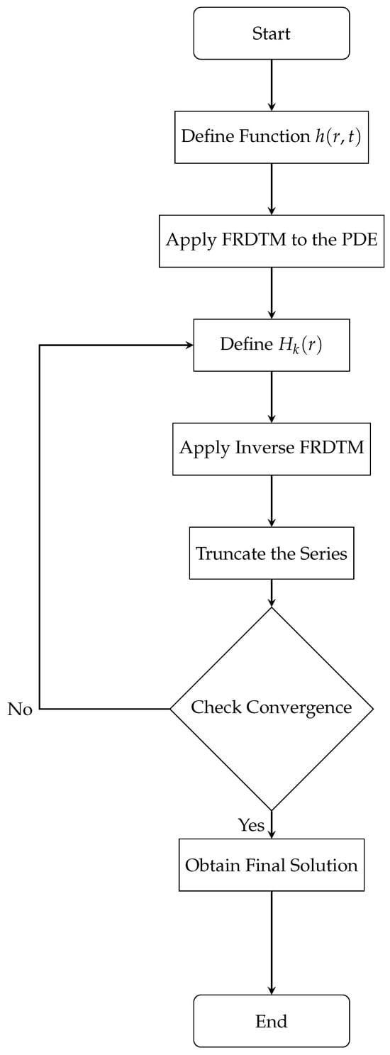
Figure 1. Flowchart of the FRDTM-based solution procedure for the time-fractional radial groundwater flow equation.

4. Application of FRDTM to Time-Fractional Radial Groundwater Flow Equation with Caputo and Atangana–Baleanu Derivatives

In this section, we apply the Fractional Reduced Differential Transform Method (FRDTM) to analytically investigate the time-fractional radial groundwater flow equation in a confined aquifer. To capture memory-dependent behaviors often observed in aquifer systems, we extend the classical model by incorporating two distinct time-fractional derivatives. First, we employ the Caputo fractional derivative, which is widely used due to its compatibility with classical initial conditions. Then, we consider the Atangana–Baleanu fractional derivative, known for its non-local and non-singular Mittag-Leffler kernel, which offers a more physically realistic description of diffusive transport with finite memory. We also explain the flow diagram Figure 2 of the FRDTM procedure to solve the time-fractional radial groundwater flow equation.

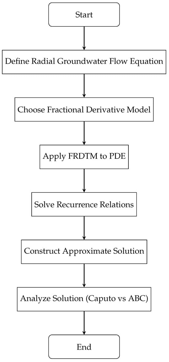
Figure 2. Flowchart of the FRDTM procedure for solving the time-fractional radial groundwater flow equation using Caputo and ABC fractional derivatives.

The governing model equation for both cases is expressed in cylindrical symmetry as a radial flow equation with a space-dependent source term:

$$\begin{array}{c}\hfill D_t^{\alpha }h(r,t)={\displaystyle \frac{T}{S}}\left({\displaystyle \frac{{\partial }^{2}h}{\partial r^2}}+{\displaystyle \frac{1}{r}}{\displaystyle \frac{\partial h}{\partial r}}\right)+q_0{e}^{-r^2},\end{array}$$

(12)

where $D_t^{\alpha }$ represents either the Caputo or Atangana–Baleanu time-fractional derivative, depending on the case considered.

Here, $h(r,t)$ denotes the hydraulic head measured in meters (m), representing the pressure level in the aquifer at radial distance r and time t. The spatial variable r lies in the radial domain $r\in [0,R]$, where $R>0$ is the outer boundary of the confined aquifer, measured in meters (m). The temporal variable $t\in [0,T]$ represents time, measured in seconds (s), where $T>0$ denotes the total simulation time.

The transmissivity T, with units of square meters per second (m²/s), quantifies the aquifer’s ability to transmit water horizontally through its saturated thickness. The storativity S is a dimensionless parameter that describes the volume of water released from or absorbed by the aquifer per unit surface area per unit change in hydraulic head. The term $q_0{e}^{-r^2}$ is a space-dependent source or sink term, where $q_0$ has units of meters per second (m/s), indicating the rate at which water is injected into or extracted from the system per unit area, and the exponential decay $e^{-r^2}$ models the spatial distribution of this influence centered around $r=0$.

Using FRDTM, we construct the solution as a series expansion in time:

$$h(r,t)=\sum _{k=0}^{\infty }{H}_k\left(r\right)t^{k\alpha }.$$

4.1. Caputo Case

We consider the time-fractional radial groundwater flow equation with a source term, given in Caputo sense as:

$${}^{C}D_t^{\alpha }h(r,t)={\displaystyle \frac{T}{S}}\left({\displaystyle \frac{{\partial }^{2}h}{\partial r^2}}+{\displaystyle \frac{1}{r}}{\displaystyle \frac{\partial h}{\partial r}}\right)+q_0{e}^{-r^2},0<\alpha \le 1,$$

(13)

subject to the initial condition:

$$h(r,0)=0.$$

Applying the Fractional Reduced Differential Transform Method (FRDTM), we express the solution in the series form:

$$h(r,t)=\sum _{k=0}^{\infty }{H}_k\left(r\right)t^{k\alpha },$$

where $H_k\left(r\right)$, is defined by

$$H_k\left(r\right)={\displaystyle \frac{1}{\mathrm{\Gamma }(k\alpha +1)}}{\left[{\displaystyle \frac{{\partial }^{k\alpha }h(r,t)}{\partial t^{k\alpha }}}\right]}_{t=t_0},k=0,1,2,\dots .$$

(14)

Substituting this series into Equation (13) and applying the FRDTM, the recurrence relation for the transformed coefficients is obtained as:

$$\begin{array}{cc}\hfill H_0\left(r\right)& =0,\hfill \end{array}$$

(15)

Equation (15) is evaluated as zero because it corresponds to the first term in the series expansion, $H_0\left(r\right)$, which represents the initial state of the system. Since the initial condition assumes no initial perturbation, i.e., $h(r,0)=0$, the first term in the series must also be zero. This aligns with the assumption that the hydraulic head is initially uniform and undisturbed, with no external forces acting on the system at $t=0$. Thus, the value of $H_0\left(r\right)$ is zero, and consequently, Equation (15) evaluates to zero.

$$\begin{array}{cc}\hfill H_k\left(r\right)& ={\displaystyle \frac{\mathrm{\Gamma }(\alpha k+1)}{\mathrm{\Gamma }(\alpha k+\alpha +1)}}\left[{\displaystyle \frac{T}{S}}\left({\displaystyle \frac{{\partial }^2{H}_{k-1}\left(r\right)}{\partial r^2}}+{\displaystyle \frac{1}{r}}{\displaystyle \frac{\partial H_{k-1}\left(r\right)}{\partial r}}\right)+{\delta }_{k,1}{q}_0{e}^{-r^2}\right],k\ge 1,\hfill \end{array}$$

(16)

where ${\delta }_{k,1}$ is the Kronecker delta, ensuring the source term is introduced only in the first term of the expansion.

The truncated solution up to the 5th term is:

$$h_5(r,t)=\sum _{k=0}^5{H}_k\left(r\right)t^{k\alpha }.$$

Using the recurrence relation (16) derived earlier and considering $h(r,0)=0$, we obtain the following explicit expressions for the terms $H_k\left(r\right)$, $k=0,1,\dots ,5$, as follows:

$$\begin{array}{cc}\hfill H_0\left(r\right)& =0,\hfill \\ \hfill H_1\left(r\right)& ={\displaystyle \frac{\mathrm{\Gamma }(\alpha +1)}{\mathrm{\Gamma }(2\alpha +1)}}{q}_0{e}^{-r^2},\hfill \\ \hfill H_2\left(r\right)& ={\displaystyle \frac{\mathrm{\Gamma }(2\alpha +1)}{\mathrm{\Gamma }(3\alpha +1)}}·{\displaystyle \frac{T}{S}}\left({\displaystyle \frac{{\partial }^2{H}_1\left(r\right)}{\partial r^2}}+{\displaystyle \frac{1}{r}}{\displaystyle \frac{\partial H_1\left(r\right)}{\partial r}}\right),\hfill \\ \hfill H_3\left(r\right)& ={\displaystyle \frac{\mathrm{\Gamma }(3\alpha +1)}{\mathrm{\Gamma }(4\alpha +1)}}·{\displaystyle \frac{T}{S}}\left({\displaystyle \frac{{\partial }^2{H}_2\left(r\right)}{\partial r^2}}+{\displaystyle \frac{1}{r}}{\displaystyle \frac{\partial H_2\left(r\right)}{\partial r}}\right),\hfill \\ \hfill H_4\left(r\right)& ={\displaystyle \frac{\mathrm{\Gamma }(4\alpha +1)}{\mathrm{\Gamma }(5\alpha +1)}}·{\displaystyle \frac{T}{S}}\left({\displaystyle \frac{{\partial }^2{H}_3\left(r\right)}{\partial r^2}}+{\displaystyle \frac{1}{r}}{\displaystyle \frac{\partial H_3\left(r\right)}{\partial r}}\right),\hfill \\ \hfill H_5\left(r\right)& ={\displaystyle \frac{\mathrm{\Gamma }(5\alpha +1)}{\mathrm{\Gamma }(6\alpha +1)}}·{\displaystyle \frac{T}{S}}\left({\displaystyle \frac{{\partial }^2{H}_4\left(r\right)}{\partial r^2}}+{\displaystyle \frac{1}{r}}{\displaystyle \frac{\partial H_4\left(r\right)}{\partial r}}\right).\hfill \end{array}$$

(17)

Thus, we get the following detailed expressions for $H_1\left(r\right)$ to $H_5\left(r\right)$:

Using the recurrence relation derived earlier and considering $h(r,0)=0$, we can obtain the explicit expressions for the terms $H_k\left(r\right)$, $k=0,1,\dots ,5$. Below are the detailed steps:

1. For $H_0\left(r\right)$: The recurrence relation for $k=0$ directly gives:

$$\begin{array}{cc}\hfill H_0\left(r\right)& =0.\hfill \end{array}$$

(18)

This is because the initial condition $h(r,0)=0$ leads to $H_0\left(r\right)=0$.

2. For $H_1\left(r\right)$: We substitute $k=1$ into the recurrence relation:

$$\begin{array}{cc}\hfill H_1\left(r\right)& ={\displaystyle \frac{\mathrm{\Gamma }(\alpha +1)}{\mathrm{\Gamma }(2\alpha +1)}}\left({\displaystyle \frac{T}{S}}\left({\displaystyle \frac{{\partial }^2{H}_0\left(r\right)}{\partial r^2}}+{\displaystyle \frac{1}{r}}{\displaystyle \frac{\partial H_0\left(r\right)}{\partial r}}\right)+{\delta }_{1,1}{q}_0{e}^{-r^2}\right).\hfill \end{array}$$

(19)

Since $H_0\left(r\right)=0$, the derivatives of $H_0\left(r\right)$ are zero. Hence, we are left with:

$$\begin{array}{cc}\hfill H_1\left(r\right)& ={\displaystyle \frac{\mathrm{\Gamma }(\alpha +1)}{\mathrm{\Gamma }(2\alpha +1)}}·q_0{e}^{-r^2}.\hfill \end{array}$$

(20)

Therefore, the expression for $H_1\left(r\right)$ is:

$$\begin{array}{cc}\hfill H_1\left(r\right)& ={\displaystyle \frac{q_0{e}^{-r^2}\mathrm{\Gamma }(\alpha +1)}{\mathrm{\Gamma }(2\alpha +1)}}.\hfill \end{array}$$

(21)

3. For $H_2\left(r\right)$: Next, we substitute $k=2$ into the recurrence relation:

$$\begin{array}{cc}\hfill H_2\left(r\right)& ={\displaystyle \frac{\mathrm{\Gamma }(2\alpha +1)}{\mathrm{\Gamma }(3\alpha +1)}}\left({\displaystyle \frac{T}{S}}\left({\displaystyle \frac{{\partial }^2{H}_1\left(r\right)}{\partial r^2}}+{\displaystyle \frac{1}{r}}{\displaystyle \frac{\partial H_1\left(r\right)}{\partial r}}\right)+{\delta }_{2,1}{q}_0{e}^{-r^2}\right).\hfill \end{array}$$

(22)

Since ${\delta }_{2,1}=0$, we only need to compute the derivatives of $H_1\left(r\right)$. Starting with:

$$\begin{array}{cc}\hfill H_1\left(r\right)& ={\displaystyle \frac{q_0{e}^{-r^2}\mathrm{\Gamma }(\alpha +1)}{\mathrm{\Gamma }(2\alpha +1)}},\hfill \end{array}$$

(23)

we compute the derivatives: First derivative:

$$\begin{array}{cc}\hfill {\displaystyle \frac{\partial H_1\left(r\right)}{\partial r}}& ={\displaystyle \frac{q_0{e}^{-r^2}\mathrm{\Gamma }(\alpha +1)}{\mathrm{\Gamma }(2\alpha +1)}}·(-2r).\hfill \end{array}$$

(24)

Second derivative:

$$\begin{array}{cc}\hfill {\displaystyle \frac{{\partial }^2{H}_1\left(r\right)}{\partial r^2}}& ={\displaystyle \frac{q_0{e}^{-r^2}\mathrm{\Gamma }(\alpha +1)}{\mathrm{\Gamma }(2\alpha +1)}}·(4r^2-2).\hfill \end{array}$$

(25)

Now substituting into the recurrence relation for $H_2\left(r\right)$:

$$\begin{array}{cc}\hfill H_2\left(r\right)& ={\displaystyle \frac{\mathrm{\Gamma }(2\alpha +1)}{\mathrm{\Gamma }(3\alpha +1)}}·{\displaystyle \frac{T}{S}}\left({\displaystyle \frac{q_0{e}^{-r^2}\mathrm{\Gamma }(\alpha +1)}{\mathrm{\Gamma }(2\alpha +1)}}·(4r^2-2)-{\displaystyle \frac{q_0{e}^{-r^2}\mathrm{\Gamma }(\alpha +1)}{\mathrm{\Gamma }(2\alpha +1)}}·2\right).\hfill \end{array}$$

(26)

Simplifying:

$$\begin{array}{cc}\hfill H_2\left(r\right)& ={\displaystyle \frac{4T{q}_0(r-1)(r+1)e^{-r^2}\mathrm{\Gamma }(\alpha +1)}{S\mathrm{\Gamma }(3\alpha +1)}}.\hfill \end{array}$$

(27)

4. For $H_3\left(r\right)$: Now, we substitute $k=3$ into the recurrence relation:

$$\begin{array}{cc}\hfill H_3\left(r\right)& ={\displaystyle \frac{\mathrm{\Gamma }(3\alpha +1)}{\mathrm{\Gamma }(4\alpha +1)}}\left({\displaystyle \frac{T}{S}}\left({\displaystyle \frac{{\partial }^2{H}_2\left(r\right)}{\partial r^2}}+{\displaystyle \frac{1}{r}}{\displaystyle \frac{\partial H_2\left(r\right)}{\partial r}}\right)\right).\hfill \end{array}$$

(28)

From the previous expression for $H_2\left(r\right)$:

$$\begin{array}{cc}\hfill H_2\left(r\right)& ={\displaystyle \frac{4T{q}_0(r^2-1)e^{-r^2}\mathrm{\Gamma }(\alpha +1)}{S\mathrm{\Gamma }(3\alpha +1)}}.\hfill \end{array}$$

(29)

Compute the first derivative ${\displaystyle \frac{\partial H_2\left(r\right)}{\partial r}}$:

$$\begin{array}{cc}\hfill {\displaystyle \frac{\partial H_2\left(r\right)}{\partial r}}& ={\displaystyle \frac{8T{q}_0\mathrm{\Gamma }(\alpha +1)}{S\mathrm{\Gamma }(3\alpha +1)}}·r{e}^{-r^2}(2-r^2)\hfill \end{array}$$

(30)

Compute the second derivative ${\displaystyle \frac{{\partial }^2{H}_2\left(r\right)}{\partial r^2}}$:

$$\begin{array}{cc}\hfill {\displaystyle \frac{{\partial }^2{H}_2\left(r\right)}{\partial r^2}}& ={\displaystyle \frac{8T{q}_0\mathrm{\Gamma }(\alpha +1)}{S\mathrm{\Gamma }(3\alpha +1)}}\left[2e^{-r^2}-7r^2{e}^{-r^2}+2r^4{e}^{-r^2}\right].\hfill \end{array}$$

(31)

substitute the first and second derivatives into the formula for $H_3\left(r\right)$:

$$\begin{array}{cc}\hfill H_3\left(r\right)& ={\displaystyle \frac{16T^2{q}_0(r^4-4r^2+2)e^{-r^2}\mathrm{\Gamma }(\alpha +1)}{S^2\mathrm{\Gamma }(4\alpha +1)}}\hfill \end{array}$$

(32)

5. For $H_4\left(r\right)$: For $k=4$, substitute into the recurrence relation:

$$\begin{array}{cc}\hfill H_4\left(r\right)& ={\displaystyle \frac{\mathrm{\Gamma }(4\alpha +1)}{\mathrm{\Gamma }(5\alpha +1)}}\left({\displaystyle \frac{T}{S}}\left({\displaystyle \frac{{\partial }^2{H}_3\left(r\right)}{\partial r^2}}+{\displaystyle \frac{1}{r}}{\displaystyle \frac{\partial H_3\left(r\right)}{\partial r}}\right)\right).\hfill \end{array}$$

(33)

Using the previous expression for $H_3\left(r\right)$:

$$\begin{array}{cc}\hfill H_3\left(r\right)& ={\displaystyle \frac{16T^2{q}_0(r^4-4r^2+2)e^{-r^2}\mathrm{\Gamma }(\alpha +1)}{S^2\mathrm{\Gamma }(4\alpha +1)}}.\hfill \end{array}$$

(34)

We compute the derivatives: - First derivative:

$$\begin{array}{cc}\hfill {\displaystyle \frac{\partial H_3\left(r\right)}{\partial r}}& =-{\displaystyle \frac{32T^2{q}_0\mathrm{\Gamma }(\alpha +1)}{S^2\mathrm{\Gamma }(4\alpha +1)}}r(r^4-6r^2+6)e^{-r^2}.\hfill \end{array}$$

(35)

Second derivative:

$$\begin{array}{cc}\hfill {\displaystyle \frac{{\partial }^2{H}_3\left(r\right)}{\partial r^2}}& ={\displaystyle \frac{32T^2{q}_0\mathrm{\Gamma }(\alpha +1)}{S^2\mathrm{\Gamma }(4\alpha +1)}}(2r^6-17r^4+30r^2-6)e^{-r^2}.\hfill \end{array}$$

(36)

Now substitute into the recurrence relation for $H_4\left(r\right)$:

$$\begin{array}{cc}\hfill H_4\left(r\right)& ={\displaystyle \frac{64T^3{q}_0(r^6-9r^4+18r^2-6)e^{-r^2}\mathrm{\Gamma }(\alpha +1)}{S^3\mathrm{\Gamma }(5\alpha +1)}}.\hfill \end{array}$$

(37)

6. For $H_5\left(r\right)$: Finally, for $k=5$, substitute into the recurrence relation:

$$\begin{array}{cc}\hfill H_5\left(r\right)& ={\displaystyle \frac{\mathrm{\Gamma }(5\alpha +1)}{\mathrm{\Gamma }(6\alpha +1)}}\left({\displaystyle \frac{T}{S}}\left({\displaystyle \frac{{\partial }^2{H}_4\left(r\right)}{\partial r^2}}+{\displaystyle \frac{1}{r}}{\displaystyle \frac{\partial H_4\left(r\right)}{\partial r}}\right)\right).\hfill \end{array}$$

(38)

Using the expression for $H_4\left(r\right)$:

$$\begin{array}{cc}\hfill H_4\left(r\right)& ={\displaystyle \frac{64T^3{q}_0(r^6-9r^4+18r^2-6)e^{-r^2}\mathrm{\Gamma }(\alpha +1)}{S^3\mathrm{\Gamma }(5\alpha +1)}}.\hfill \end{array}$$

(39)

We compute the derivatives: - First derivative:

$$\begin{array}{c}\hfill {\displaystyle \frac{\partial H_4\left(r\right)}{\partial r}}=-{\displaystyle \frac{128T^3{q}_0\mathrm{\Gamma }(\alpha +1)}{S^3\mathrm{\Gamma }(5\alpha +1)}}r(r^6-12r^4+36r^2-24)e^{-r^2}.\end{array}$$

(40)

Second derivative:

$$\begin{array}{c}\hfill {\displaystyle \frac{{\partial }^2{H}_4\left(r\right)}{\partial r^2}}={\displaystyle \frac{128T^3{q}_0\mathrm{\Gamma }(\alpha +1)}{S^3\mathrm{\Gamma }(5\alpha +1)}}(2r^8-31r^6+132r^4-156r^2+24)e^{-r^2}.\end{array}$$

(41)

By substituting into the recurrence relation for $H_5\left(r\right)$ we get:

$$\begin{array}{cc}\hfill H_5\left(r\right)& ={\displaystyle \frac{256T^4{q}_0(r^8-16r^6+72r^4-96r^2+24)e^{-r^2}\mathrm{\Gamma }(\alpha +1)}{S^4\mathrm{\Gamma }(6\alpha +1)}}.\hfill \end{array}$$

(42)

Now, we can use these results in the final expression for the approximate solution:

$$\begin{array}{c}\hfill \begin{array}{cc}\hfill h_5(r,t)& =H_1\left(r\right)t^{\alpha }+H_2\left(r\right)t^{2\alpha }+H_3\left(r\right)t^{3\alpha }+H_4\left(r\right)t^{4\alpha }+H_5\left(r\right)t^{5\alpha }\hfill \\ \hfill & ={\displaystyle \frac{q_0{e}^{-r^2}\mathrm{\Gamma }(\alpha +1)}{\mathrm{\Gamma }(2\alpha +1)}}{t}^{\alpha }+{\displaystyle \frac{4T{q}_0(r-1)(r+1)e^{-r^2}\mathrm{\Gamma }(\alpha +1)}{S\mathrm{\Gamma }(3\alpha +1)}}{t}^{2\alpha }\hfill \\ \hfill & +{\displaystyle \frac{16T^2{q}_0(r^4-4r^2+2)e^{-r^2}\mathrm{\Gamma }(\alpha +1)}{S^2\mathrm{\Gamma }(4\alpha +1)}}{t}^{3\alpha }\hfill \\ \hfill & +{\displaystyle \frac{64T^3{q}_0(r^6-9r^4+18r^2-6)e^{-r^2}\mathrm{\Gamma }(\alpha +1)}{S^3\mathrm{\Gamma }(5\alpha +1)}}{t}^{4\alpha }\hfill \\ \hfill & +{\displaystyle \frac{256T^4{q}_0(r^8-16r^6+72r^4-96r^2+24)e^{-r^2}\mathrm{\Gamma }(\alpha +1)}{S^4\mathrm{\Gamma }(6\alpha +1)}}{t}^{5\alpha }.\hfill \end{array}\end{array}$$

(43)

4.2. Atangana–Baleanu Caputo Case

We now consider the same radial groundwater flow equation in the sense of the Atangana–Baleanu Caputo (ABC) fractional derivative:

$${}^{\mathit{ABC}}D_t^{\alpha }h(r,t)={\displaystyle \frac{T}{S}}\left({\displaystyle \frac{{\partial }^{2}h}{\partial r^2}}+{\displaystyle \frac{1}{r}}{\displaystyle \frac{\partial h}{\partial r}}\right)+q_0{e}^{-r^2},0<\alpha \le 1,$$

(44)

subject to the initial condition:

$$h(r,0)=0.$$

In the ABC derivative, the kernel is non-singular and non-local, and the fractional operator is defined in the Caputo sense using the Mittag–Leffler function as its kernel. The Fractional Reduced Differential Transform Method (FRDTM) can be adapted accordingly by modifying the recurrence relation:

$$\begin{array}{cc}\hfill H_{k+1}\left(r\right)& ={\displaystyle \frac{1-\alpha }{B\left(\alpha \right)}}{H}_k\left(r\right)+{\displaystyle \frac{\alpha }{B\left(\alpha \right)\mathrm{\Gamma }\left(\right(k+1)\alpha +1)}}\left[{\displaystyle \frac{T}{S}}\left({\displaystyle \frac{{\partial }^2{H}_k\left(r\right)}{\partial r^2}}+{\displaystyle \frac{1}{r}}{\displaystyle \frac{\partial H_k\left(r\right)}{\partial r}}\right)+{\delta }_{k,0}{q}_0{e}^{-r^2}\right],\hfill \end{array}$$

(45)

where $B\left(\alpha \right)=1-\alpha +{\displaystyle \frac{\alpha }{\mathrm{\Gamma }\left(\alpha \right)}}$, and ${\delta }_{k,0}$ is the Kronecker delta. Using the above recurrence relation, and the initial condition $h(r,0)=0\Rightarrow H_0\left(r\right)=0$, we compute the first few terms:

1. For $H_0\left(r\right)$: The recurrence relation for $k=0$ directly gives:

$$\begin{array}{cc}\hfill H_0\left(r\right)& =0.\hfill \end{array}$$

(46)

This is because the initial condition $h(r,0)=0$ implies that $H_0\left(r\right)=0$.

2. For $H_1\left(r\right)$: For $k=1$, the recurrence relation becomes:

$$\begin{array}{cc}\hfill H_1\left(r\right)& ={\displaystyle \frac{1-\alpha }{B\left(\alpha \right)}}{H}_0\left(r\right)+{\displaystyle \frac{\alpha }{B\left(\alpha \right)\mathrm{\Gamma }(\alpha +1)}}\left[{\displaystyle \frac{T}{S}}\left({\displaystyle \frac{{\partial }^2{H}_0\left(r\right)}{\partial r^2}}+{\displaystyle \frac{1}{r}}{\displaystyle \frac{\partial H_0\left(r\right)}{\partial r}}\right)+{\delta }_{0,0}{q}_0{e}^{-r^2}\right].\hfill \end{array}$$

(47)

Since $H_0\left(r\right)=0$, the first part of the equation vanishes, and we are left with:

$$\begin{array}{cc}\hfill H_1\left(r\right)& ={\displaystyle \frac{\alpha q_0{e}^{-r^2}}{B\left(\alpha \right)\mathrm{\Gamma }(\alpha +1)}}.\hfill \end{array}$$

(48)

3. For $H_2\left(r\right)$: Now, for $k=2$, we substitute $H_1\left(r\right)$ into the recurrence relation:

$$\begin{array}{cc}\hfill H_2\left(r\right)& ={\displaystyle \frac{1-\alpha }{B\left(\alpha \right)}}{H}_1\left(r\right)+{\displaystyle \frac{\alpha }{B\left(\alpha \right)\mathrm{\Gamma }(2\alpha +1)}}\left[{\displaystyle \frac{T}{S}}\left({\displaystyle \frac{{\partial }^2{H}_1\left(r\right)}{\partial r^2}}+{\displaystyle \frac{1}{r}}{\displaystyle \frac{\partial H_1\left(r\right)}{\partial r}}\right)+{\delta }_{1,0}{q}_0{e}^{-r^2}\right].\hfill \end{array}$$

(49)

Since ${\delta }_{1,0}=0$, the second part of the equation vanishes. We now compute the derivatives of $H_1\left(r\right)$:

$$\begin{array}{cc}\hfill H_1\left(r\right)& ={\displaystyle \frac{\alpha q_0{e}^{-r^2}}{B\left(\alpha \right)\mathrm{\Gamma }(\alpha +1)}}.\hfill \end{array}$$

(50)

First derivative:

$$\begin{array}{cc}\hfill {\displaystyle \frac{\partial H_1\left(r\right)}{\partial r}}& ={\displaystyle \frac{-2r\alpha q_0{e}^{-r^2}}{B\left(\alpha \right)\mathrm{\Gamma }(\alpha +1)}}.\hfill \end{array}$$

(51)

Second derivative:

$$\begin{array}{cc}\hfill {\displaystyle \frac{{\partial }^2{H}_1\left(r\right)}{\partial r^2}}& ={\displaystyle \frac{2r^2\alpha q_0{e}^{-r^2}}{B\left(\alpha \right)\mathrm{\Gamma }(\alpha +1)}}-{\displaystyle \frac{2\alpha q_0{e}^{-r^2}}{B\left(\alpha \right)\mathrm{\Gamma }(\alpha +1)}}.\hfill \end{array}$$

(52)

Substituting these into the recurrence relation for $H_2\left(r\right)$, we get:

$$\begin{array}{cc}\hfill H_2\left(r\right)& ={\displaystyle \frac{4\alpha T{q}_0(r-1)(r+1)e^{-r^2}}{B\left(\alpha \right)S\mathrm{\Gamma }(2\alpha +1)}}.\hfill \end{array}$$

(53)

4. For $H_3\left(r\right)$: For $k=3$, substitute $H_2\left(r\right)$ into the recurrence relation:

$$\begin{array}{cc}\hfill H_3\left(r\right)& ={\displaystyle \frac{1-\alpha }{B\left(\alpha \right)}}{H}_2\left(r\right)+{\displaystyle \frac{\alpha }{B\left(\alpha \right)\mathrm{\Gamma }(3\alpha +1)}}\left[{\displaystyle \frac{T}{S}}\left({\displaystyle \frac{{\partial }^2{H}_2\left(r\right)}{\partial r^2}}+{\displaystyle \frac{1}{r}}{\displaystyle \frac{\partial H_2\left(r\right)}{\partial r}}\right)+{\delta }_{2,0}{q}_0{e}^{-r^2}\right].\hfill \end{array}$$

(54)

Since ${\delta }_{2,0}=0$, we need to compute the derivatives of $H_2\left(r\right)$. Using:

$$\begin{array}{cc}\hfill H_2\left(r\right)& ={\displaystyle \frac{4\alpha T{q}_0(r-1)(r+1)e^{-r^2}}{B\left(\alpha \right)S\mathrm{\Gamma }(2\alpha +1)}},\hfill \end{array}$$

(55)

we compute the derivatives: - First derivative:

$$\begin{array}{cc}\hfill {\displaystyle \frac{\partial H_2\left(r\right)}{\partial r}}& ={\displaystyle \frac{8\alpha T{q}_0{e}^{-r^2}}{B\left(\alpha \right)S\mathrm{\Gamma }(2\alpha +1)}}·r{e}^{-r^2}(2-r^2).\hfill \end{array}$$

(56)

Second derivative:

$$\begin{array}{cc}\hfill {\displaystyle \frac{{\partial }^2{H}_2\left(r\right)}{\partial r^2}}& ={\displaystyle \frac{8\alpha T{q}_0{e}^{-r^2}}{B\left(\alpha \right)S\mathrm{\Gamma }(2\alpha +1)}}\left[2e^{-r^2}-7r^2{e}^{-r^2}+2r^4{e}^{-r^2}\right].\hfill \end{array}$$

(57)

By substituting these into the recurrence relation for $H_3\left(r\right)$, we get:

$$\begin{array}{cc}\hfill H_3\left(r\right)& ={\displaystyle \frac{16\alpha T^2{q}_0(r^4-4r^2+2)e^{-r^2}}{B\left(\alpha \right)S^2\mathrm{\Gamma }(3\alpha +1)}}.\hfill \end{array}$$

(58)

5. For $H_4\left(r\right)$: For $k=4$, substitute $H_3\left(r\right)$ into the recurrence relation:

$$\begin{array}{cc}\hfill H_4\left(r\right)& ={\displaystyle \frac{1-\alpha }{B\left(\alpha \right)}}{H}_3\left(r\right)+{\displaystyle \frac{\alpha }{B\left(\alpha \right)\mathrm{\Gamma }(4\alpha +1)}}\left[{\displaystyle \frac{T}{S}}\left({\displaystyle \frac{{\partial }^2{H}_3\left(r\right)}{\partial r^2}}+{\displaystyle \frac{1}{r}}{\displaystyle \frac{\partial H_3\left(r\right)}{\partial r}}\right)+{\delta }_{3,0}{q}_0{e}^{-r^2}\right].\hfill \end{array}$$

(59)

Since ${\delta }_{3,0}=0$, we need to compute the derivatives of $H_3\left(r\right)$. Using:

$$\begin{array}{cc}\hfill H_3\left(r\right)& ={\displaystyle \frac{16\alpha T^2{q}_0(r^4-4r^2+2)e^{-r^2}}{B\left(\alpha \right)S^2\mathrm{\Gamma }(3\alpha +1)}},\hfill \end{array}$$

(60)

we compute the derivatives: - First derivative:

$$\begin{array}{cc}\hfill {\displaystyle \frac{\partial H_3\left(r\right)}{\partial r}}& =-{\displaystyle \frac{32\alpha T^2{q}_0{e}^{-r^2}}{B\left(\alpha \right)S^2\mathrm{\Gamma }(3\alpha +1)}}r(r^4-6r^2+6)e^{-r^2}\hfill \end{array}$$

(61)

Second derivative:

$$\begin{array}{cc}\hfill {\displaystyle \frac{{\partial }^2{H}_3\left(r\right)}{\partial r^2}}& ={\displaystyle \frac{32\alpha T^2{q}_0{e}^{-r^2}}{B\left(\alpha \right)S^2\mathrm{\Gamma }(3\alpha +1)}}(2r^6-17r^4+30r^2-6)e^{-r^2}.\hfill \end{array}$$

(62)

By substituting these into the recurrence relation for $H_4\left(r\right)$, we get:

$$\begin{array}{cc}\hfill H_4\left(r\right)& ={\displaystyle \frac{64\alpha T^3{q}_0(r^6-9r^4+18r^2-6)e^{-r^2}}{B\left(\alpha \right)S^3\mathrm{\Gamma }(4\alpha +1)}}.\hfill \end{array}$$

(63)

6. For $H_5\left(r\right)$: Finally, for $k=5$, substitute $H_4\left(r\right)$ into the recurrence relation:

$$\begin{array}{cc}\hfill H_5\left(r\right)& ={\displaystyle \frac{1-\alpha }{B\left(\alpha \right)}}{H}_4\left(r\right)+{\displaystyle \frac{\alpha }{B\left(\alpha \right)\mathrm{\Gamma }(5\alpha +1)}}\left[{\displaystyle \frac{T}{S}}\left({\displaystyle \frac{{\partial }^2{H}_4\left(r\right)}{\partial r^2}}+{\displaystyle \frac{1}{r}}{\displaystyle \frac{\partial H_4\left(r\right)}{\partial r}}\right)+{\delta }_{4,0}{q}_0{e}^{-r^2}\right].\hfill \end{array}$$

(64)

Since ${\delta }_{4,0}=0$, we compute the derivatives of $H_4\left(r\right)$. Using:

$$\begin{array}{cc}\hfill H_4\left(r\right)& ={\displaystyle \frac{64\alpha T^3{q}_0(r^6-9r^4+18r^2-6)e^{-r^2}}{B\left(\alpha \right)S^3\mathrm{\Gamma }(4\alpha +1)}},\hfill \end{array}$$

(65)

we compute the derivatives: - First derivative:

$$\begin{array}{cc}\hfill {\displaystyle \frac{\partial H_4\left(r\right)}{\partial r}}& =-{\displaystyle \frac{128\alpha T^3{q}_0{e}^{-r^2}}{B\left(\alpha \right)S^3\mathrm{\Gamma }(4\alpha +1)}}r(r^6-12r^4+36r^2-24)e^{-r^2}.\hfill \end{array}$$

(66)

Second derivative:

$$\begin{array}{cc}\hfill {\displaystyle \frac{{\partial }^2{H}_4\left(r\right)}{\partial r^2}}& ={\displaystyle \frac{128\alpha T^3{q}_0{e}^{-r^2}}{B\left(\alpha \right)S^3\mathrm{\Gamma }(4\alpha +1)}}(2r^8-31r^6+132r^4-156r^2+24)e^{-r^2}.\hfill \end{array}$$

(67)

By substituting these into the recurrence relation for $H_5\left(r\right)$, we get:

$$\begin{array}{cc}\hfill H_5\left(r\right)& ={\displaystyle \frac{256\alpha T^4{q}_0(r^8-16r^6+72r^4-96r^2+24)e^{-r^2}}{B\left(\alpha \right)S^4\mathrm{\Gamma }(5\alpha +1)}}.\hfill \end{array}$$

(68)

Thus, the approximate solution up to the 5th term becomes:

$$\begin{array}{cc}\hfill h_5(r,t)& =H_1\left(r\right)t^{\alpha }+H_2\left(r\right)t^{2\alpha }+H_3\left(r\right)t^{3\alpha }+H_4\left(r\right)t^{4\alpha }+H_5\left(r\right)t^{5\alpha }\hfill \\ \hfill & ={\displaystyle \frac{\alpha q_0{e}^{-r^2}}{B\left(\alpha \right)\mathrm{\Gamma }(\alpha +1)}}{t}^{\alpha }+{\displaystyle \frac{4\alpha T{q}_0(r-1)(r+1)e^{-r^2}}{B\left(\alpha \right)S\mathrm{\Gamma }(2\alpha +1)}}{t}^{2\alpha }\hfill \\ \hfill & +{\displaystyle \frac{16\alpha T^2{q}_0(r^4-4r^2+2)e^{-r^2}}{B\left(\alpha \right)S^2\mathrm{\Gamma }(3\alpha +1)}}{t}^{3\alpha }\hfill \\ \hfill & +{\displaystyle \frac{64\alpha T^3{q}_0(r^6-9r^4+18r^2-6)e^{-r^2}}{B\left(\alpha \right)S^3\mathrm{\Gamma }(4\alpha +1)}}{t}^{4\alpha }\hfill \\ \hfill & +{\displaystyle \frac{256\alpha T^4{q}_0(r^8-16r^6+72r^4-96r^2+24)e^{-r^2}}{B\left(\alpha \right)S^4\mathrm{\Gamma }(5\alpha +1)}}{t}^{5\alpha }.\hfill \end{array}$$

(69)

5. Convergence and Stability Analysis

In this section, we rigorously examine the convergence and stability properties of the solutions obtained by applying the Fractional Reduced Differential Transform Method (FRDTM) to the time-fractional radial groundwater flow equation. Since the governing model can be formulated using different types of fractional derivatives, namely the Caputo and the Atangana–Baleanu (ABC) operators, we provide a separate analysis for each case.

First, we investigate the Caputo derivative case, where we establish the recurrence relations for the FRDTM coefficients, analyze the asymptotic behavior of the resulting series, and demonstrate convergence using properties of the Gamma function and Mittag–Leffler functions. We then study the stability of the Caputo-based FRDTM solution under small perturbations in the initial condition using a norm-based energy method. Next, we turn to the Atangana–Baleanu (ABC) derivative formulation. Here, we derive the corresponding FRDTM recurrence relation, prove uniform convergence of the solution series, and again employ a perturbation analysis to confirm stability in the presence of initial condition uncertainties.

Through this comparative study, we establish that the FRDTM produces solutions that are not only convergent but also stable in both Caputo and ABC fractional derivative settings, thereby confirming its reliability and robustness for simulating time-fractional groundwater flow dynamics.

5.1. Convergence and Stability Analysis in the Caputo Case

We consider the time-fractional radial groundwater flow equation in the Caputo sense:

$${}^{C}D_t^{\alpha }h(r,t)={\displaystyle \frac{T}{S}}\left({\displaystyle \frac{{\partial }^{2}h}{\partial r^2}}+{\displaystyle \frac{1}{r}}{\displaystyle \frac{\partial h}{\partial r}}\right)+q_0{e}^{-r^2},0<\alpha \le 1.$$

(70)

Using the FRDTM, the solution is expressed in series form as:

$$h(r,t)=\sum _{k=0}^{\infty }{H}_k\left(r\right)t^{k\alpha },\mathrm{with}\mathrm{truncated}\mathrm{form}{h}_n(r,t)=\sum _{k=0}^n{H}_k\left(r\right)t^{k\alpha }.$$

5.1.1. Convergence in the Caputo Case

The convergence of the FRDTM solution series

$$h(r,t)=\sum _{k=0}^{\infty }{H}_k\left(r\right)t^{k\alpha }$$

depends on the behavior of both the series coefficients $H_k\left(r\right)$ and the time-power terms $t^{k\alpha }$ as $k\to \infty$. Applying FRDTM to the Caputo-formulated time-fractional radial groundwater flow equation leads to the recurrence relation:

$$\begin{array}{c}\hfill H_{k+1}\left(r\right)={\displaystyle \frac{\mathrm{\Gamma }(k\alpha +1)}{\mathrm{\Gamma }\left(\right(k+1)\alpha +1)}}\left[{\displaystyle \frac{T}{S}}\left({\displaystyle \frac{{\partial }^2{H}_k\left(r\right)}{\partial r^2}}+{\displaystyle \frac{1}{r}}{\displaystyle \frac{\partial H_k\left(r\right)}{\partial r}}\right)+{\delta }_{k,0}{q}_0{e}^{-r^2}\right],\end{array}$$

(71)

where ${\delta }_{k,0}$ is the Kronecker delta and $0<\alpha \le 1$. The gamma ratio

$${\displaystyle \frac{\mathrm{\Gamma }(k\alpha +1)}{\mathrm{\Gamma }\left(\right(k+1)\alpha +1)}}\sim {\displaystyle \frac{1}{{(k+1)}^{\alpha }}}$$

for large k, which indicates factorial-type decay in the recurrence. This decay plays a key role in damping the growth of higher-order terms.

Moreover, assuming that: the initial condition $h(r,0)=0$ implies $H_0\left(r\right)=0$, the source term $q_0{e}^{-r^2}$ is smooth and bounded for $r\in [0,R]$ and the spatial derivatives $\partial H_k/\partial r$ and ${\partial }^2{H}_k/\partial r^2$ remain bounded (due to the regularity of the PDE and physical conditions of the confined aquifer), then the recurrence will produce bounded $H_k\left(r\right)$ terms that decrease in magnitude for large k. Each successive term in the series is additionally multiplied by $t^{k\alpha }$, which is increasingly small for any fixed $t\in [0,T_0]$ and large k, since $\alpha >0$.

Hence, we conclude that the infinite series:

$$\sum _{k=0}^{\infty }{H}_k\left(r\right)t^{k\alpha }$$

is absolutely and uniformly convergent for all $(r,t)\in [0,R]\times [0,T_0]$, for any finite $R,T_0>0$. This ensures the FRDTM solution $h(r,t)$ is well-defined and represents a valid approximation to the original time-fractional PDE.

Alternatively, the convergence can be established using a comparison with the Mittag–Leffler function $E_{\alpha }(·)$. Noting that:

$$\begin{array}{c}\hfill |H_k\left(r\right)|\le M·\left({\displaystyle \frac{C}{\mathrm{\Gamma }(1+k\alpha )}}\right),\mathrm{for}\mathrm{some}M,C>0,\end{array}$$

(72)

we observe:

$$\begin{array}{c}\hfill \left|h(r,t)\right|\le \sum _{k=0}^{\infty }{\displaystyle \frac{M{C}^k{t}^{k\alpha }}{\mathrm{\Gamma }(1+k\alpha )}}=M·E_{\alpha }\left(C{t}^{\alpha }\right),\end{array}$$

(73)

which is bounded for any fixed t, as the Mittag–Leffler function grows sub-exponentially.

This approach not only confirms the convergence, but also gives an upper bound on the solution behavior, reinforcing the theoretical soundness and numerical stability of the FRDTM solution in the Caputo case.

5.1.2. Generalized Stability Analysis for FRDTM in Caputo Case

We perform a generalized stability analysis of the Fractional Reduced Differential Transform Method (FRDTM) to ensure that it is robust under a broad range of perturbations. Perturbations can arise from various sources, including initial conditions, boundary conditions, external forcing terms, numerical errors, model inaccuracies, and sensitivity to system parameters. This section outlines the stability of FRDTM under such disturbances, ensuring that the method remains numerically robust in practical simulation environments.

Stability Under Perturbations in Initial Conditions

Let us first consider the case where perturbations occur in the initial conditions. Suppose the initial state $h(r,0)=0$ is perturbed by a function $ϵ\left(r\right)$, such that:

$$\tilde{h}(r,0)=ϵ\left(r\right),\parallel ϵ\left(r\right)\parallel \le \epsilon ,\mathrm{where}\parallel ·\parallel \mathrm{denotes}\mathrm{a}\mathrm{suitable}\mathrm{norm}\mathrm{over}[0,R].$$

Applying the FRDTM, the solution is expressed as:

$$\begin{array}{c}\hfill h(r,t)=\sum _{k=0}^{\infty }{H}_k\left(r\right)t^{k\alpha },\tilde{h}(r,t)=\sum _{k=0}^{\infty }{\tilde{H}}_k\left(r\right)t^{k\alpha }.\end{array}$$

(74)

We define the error function in coefficient space as:

$$\begin{array}{c}\hfill E_k\left(r\right)={\tilde{H}}_k\left(r\right)-H_k\left(r\right),\end{array}$$

(75)

and let the total error function be:

$$\begin{array}{c}\hfill e_n(r,t)=\sum _{k=0}^n{E}_k\left(r\right)t^{k\alpha }.\end{array}$$

(76)

The recurrence relation for the coefficients $H_k\left(r\right)$ is given by:

$$\begin{array}{c}\hfill H_{k+1}\left(r\right)={\displaystyle \frac{\mathrm{\Gamma }(k\alpha +1)}{\mathrm{\Gamma }\left(\right(k+1)\alpha +1)}}\left[{\displaystyle \frac{T}{S}}\left({\displaystyle \frac{{\partial }^2{H}_k\left(r\right)}{\partial r^2}}+{\displaystyle \frac{1}{r}}{\displaystyle \frac{\partial H_k\left(r\right)}{\partial r}}\right)+{\delta }_{k,0}{q}_0{e}^{-r^2}\right],\end{array}$$

(77)

and similarly for the perturbed coefficients ${\tilde{H}}_k\left(r\right)$. The recurrence relation for the error function $E_k\left(r\right)$ is:

$$\begin{array}{c}\hfill E_{k+1}\left(r\right)={\displaystyle \frac{\mathrm{\Gamma }(k\alpha +1)}{\mathrm{\Gamma }\left(\right(k+1)\alpha +1)}}·{\displaystyle \frac{T}{S}}\left({\displaystyle \frac{{\partial }^2{E}_k\left(r\right)}{\partial r^2}}+{\displaystyle \frac{1}{r}}{\displaystyle \frac{\partial E_k\left(r\right)}{\partial r}}\right).\end{array}$$

(78)

To analyze the stability of the solution under these perturbations, we apply the $L^2$-norm over $[0,R]$ and use the energy method:

$$\begin{array}{c}\hfill \parallel E_{k+1}\parallel \le {\displaystyle \frac{T}{S}}·{\displaystyle \frac{\mathrm{\Gamma }(k\alpha +1)}{\mathrm{\Gamma }\left(\right(k+1)\alpha +1)}}·∥{\displaystyle \frac{{\partial }^2{E}_k}{\partial r^2}}+{\displaystyle \frac{1}{r}}{\displaystyle \frac{\partial E_k}{\partial r}}∥\le C·\parallel E_k\parallel ,\end{array}$$

(79)

where $C>0$ is a constant depending on the differential operator and the boundedness of derivatives in the physical domain. Using mathematical induction, we get:

$$\begin{array}{c}\hfill \parallel E_k\parallel \le C^k\parallel ϵ\left(r\right)\parallel \le C^k\epsilon ,\end{array}$$

(80)

which implies that the total error satisfies:

$$\begin{array}{c}\hfill \parallel e_n(r,t)\parallel \le \epsilon \sum _{k=0}^n{\left(C{t}^{\alpha }\right)}^k=\epsilon ·{\displaystyle \frac{1-{\left(C{t}^{\alpha }\right)}^{n+1}}{1-C{t}^{\alpha }}},\mathrm{for}C{t}^{\alpha }<1.\end{array}$$

(81)

Thus, the total error in the approximate solution is uniformly bounded, and small perturbations in the initial condition do not grow unbounded over time, proving that the FRDTM is stable under initial condition perturbations.

Stability Under Perturbations in Boundary Conditions and External Forces

Next, we extend the stability analysis to account for disturbances originating from boundary conditions and external forcing terms. Let the boundary conditions at $r=0$ and $r=R$ be perturbed by small functions:

$$\begin{array}{c}\hfill h(0,t)={ϵ}_0\left(t\right),h(R,t)={ϵ}_R\left(t\right),\end{array}$$

(82)

where $\parallel {ϵ}_0\left(t\right)\parallel \le {\epsilon }_0$ and $\parallel {ϵ}_R\left(t\right)\parallel \le {\epsilon }_R$, representing small disturbances at the boundaries. Similarly, we model the source term perturbation as:

$$\begin{array}{c}\hfill q(r,t)=q_0{e}^{-r^2}+\delta q(r,t),\end{array}$$

(83)

where $\parallel \delta q(r,t)\parallel \le {\epsilon }_q$. The recurrence relations for the perturbed solution coefficients due to boundary and source term perturbations are:

$$\begin{array}{c}\hfill E_{k+1}\left(r\right)={\displaystyle \frac{\mathrm{\Gamma }(k\alpha +1)}{\mathrm{\Gamma }\left(\right(k+1)\alpha +1)}}·{\displaystyle \frac{T}{S}}\left({\displaystyle \frac{{\partial }^2{E}_k\left(r\right)}{\partial r^2}}+{\displaystyle \frac{1}{r}}{\displaystyle \frac{\partial E_k\left(r\right)}{\partial r}}\right)+{\delta }_{k,0}·{\displaystyle \frac{T}{S}}\delta q(r,t).\end{array}$$

(84)

As shown for initial condition perturbations, the perturbations from boundary conditions and external forces lead to bounded errors:

$$\begin{array}{c}\hfill \parallel E_k\left(r\right)\parallel \le C^{k}max({\epsilon }_0,{\epsilon }_R,{\epsilon }_q),\end{array}$$

(85)

which ensures that the total error remains bounded under these additional disturbances. The total error is then given by:

$$\begin{array}{c}\hfill \parallel e_n(r,t)\parallel \le \epsilon ·{\displaystyle \frac{1-{\left(C{t}^{\alpha }\right)}^{n+1}}{1-C{t}^{\alpha }}},\end{array}$$

(86)

where $\epsilon$ now accounts for all disturbances (from initial conditions, boundary conditions, and external forces).

Stability Under Model Inaccuracies and Numerical Errors

In practical simulation environments, numerical errors and model inaccuracies also contribute to the overall perturbation. Let the model perturbation be $\delta h(r,t)$, which represents small discrepancies between the idealized model and the real system. The recurrence relation for this perturbation is:

$$\begin{array}{c}\hfill E_{k+1}\left(r\right)={\displaystyle \frac{\mathrm{\Gamma }(k\alpha +1)}{\mathrm{\Gamma }\left(\right(k+1)\alpha +1)}}·{\displaystyle \frac{T}{S}}\left({\displaystyle \frac{{\partial }^2{E}_k\left(r\right)}{\partial r^2}}+{\displaystyle \frac{1}{r}}{\displaystyle \frac{\partial E_k\left(r\right)}{\partial r}}\right)+{\delta }_{k,0}\delta h(r,t).\end{array}$$

(87)

Assuming the model inaccuracies are bounded by ${\epsilon }_m$, we find:

$$\begin{array}{c}\hfill \parallel E_k\left(r\right)\parallel \le C^k{\epsilon }_m.\end{array}$$

(88)

Thus, similar to other perturbations, the total error remains bounded, and the FRDTM continues to be stable.

The generalized stability analysis confirms that the FRDTM is robust against a wide range of perturbations, including those from initial conditions, boundary conditions, external forcing, numerical errors, and model inaccuracies. In all cases, the total error remains uniformly bounded, ensuring the stability of the method in both theoretical and practical simulation settings. These findings guarantee that the FRDTM can be reliably applied to real-world groundwater flow problems, even when subjected to general disturbances.

5.1.3. Convergence in the ABC Case

We consider the time-fractional radial groundwater flow model with the Atangana–Baleanu fractional derivative (in Caputo sense), given by:

$$\begin{array}{c}\hfill {}^{\mathit{ABC}}D_t^{\alpha }h(r,t)={\displaystyle \frac{T}{S}}\left({\displaystyle \frac{{\partial }^{2}h}{\partial r^2}}+{\displaystyle \frac{1}{r}}{\displaystyle \frac{\partial h}{\partial r}}\right)+q_0{e}^{-r^2},0<\alpha <1.\end{array}$$

(89)

Applying the Fractional Reduced Differential Transform Method (FRDTM) to the ABC formulation yields the recurrence relation:

$$\begin{array}{c}\hfill H_{k+1}\left(r\right)={\displaystyle \frac{B\left(\alpha \right)}{1-\alpha }}\left[{\displaystyle \frac{T}{S}}\left({\displaystyle \frac{{\partial }^2{H}_k\left(r\right)}{\partial r^2}}+{\displaystyle \frac{1}{r}}{\displaystyle \frac{\partial H_k\left(r\right)}{\partial r}}\right)+{\delta }_{k,0}{q}_0{e}^{-r^2}\right]·{\displaystyle \frac{\mathrm{\Gamma }(k\alpha +1)}{\mathrm{\Gamma }\left(\right(k+1)\alpha +1)}},\end{array}$$

(90)

where $B\left(\alpha \right)$ is a normalization constant related to the Mittag–Leffler kernel of the ABC operator, and ${\delta }_{k,0}$ is the Kronecker delta.

As $k\to \infty$, the ratio of gamma functions behaves asymptotically as:

$${\displaystyle \frac{\mathrm{\Gamma }(k\alpha +1)}{\mathrm{\Gamma }\left(\right(k+1)\alpha +1)}}\sim {\displaystyle \frac{1}{{(k+1)}^{\alpha }}},$$

ensuring a rapid decay in the magnitude of the recurrence terms.

Furthermore, under the assumption that the spatial domain $r\in [0,R]$ is bounded, the initial condition is $h(r,0)=0$, leading to $H_0\left(r\right)=0$, the source term $q_0{e}^{-r^2}$ is smooth and bounded, and the recursive spatial terms $\partial H_k/\partial r$ and ${\partial }^2{H}_k/\partial r^2$ remain bounded for each k, it follows that the sequence $\left\{H_k\left(r\right)\right\}$ remains bounded and decays for large k.

Hence, the full series solution:

$$h(r,t)=\sum _{k=0}^{\infty }{H}_k\left(r\right)t^{k\alpha }$$

is absolutely and uniformly convergent for $t\in [0,T_0]$ and $r\in [0,R]$, due to the boundedness of $H_k\left(r\right)$ and decay of the gamma function in the denominator.

For a more quantitative assessment, we consider:

$$\begin{array}{c}\hfill |H_k\left(r\right)|\le C·{\displaystyle \frac{M^k}{\mathrm{\Gamma }(1+k\alpha )}},\mathrm{for}\mathrm{constants}C,M>0.\end{array}$$

(91)

This gives a bound on the solution:

$$\begin{array}{c}\hfill \left|h(r,t)\right|\le C\sum _{k=0}^{\infty }{\displaystyle \frac{{\left(M{t}^{\alpha }\right)}^k}{\mathrm{\Gamma }(1+k\alpha )}}=C·E_{\alpha }\left(M{t}^{\alpha }\right),\end{array}$$

(92)

where $E_{\alpha }(·)$ is the one-parameter Mittag–Leffler function, known to be bounded for any finite argument.

This confirms that the ABC-FRDTM solution converges absolutely and uniformly for all $(r,t)\in [0,R]\times [0,T_0]$, ensuring a valid and stable analytical approximation to the original fractional PDE.

Generalized Stability Under the ABC Fractional Derivative

In this section, we extend the stability analysis for the Atangana–Baleanu–Caputo (ABC) fractional derivative, considering perturbations not only in initial conditions but also in boundary conditions, external forcing terms, model inaccuracies, and numerical errors. This ensures that the FRDTM remains stable under a wide range of practical disturbances, which are common in real-world simulation environments.

Stability Under Perturbations in Initial Conditions

Consider the initial condition $h(r,0)=0$, and let the initial condition be perturbed by a small function $ϵ\left(r\right)$, such that:

$$\begin{array}{c}\hfill \tilde{h}(r,0)=ϵ\left(r\right),\parallel ϵ\left(r\right)\parallel \le \epsilon ,\end{array}$$

(93)

where $\parallel ·\parallel$ denotes a suitable norm over the spatial domain $r\in [0,R]$. The FRDTM solution is expressed as:

$$\begin{array}{c}\hfill h(r,t)=\sum _{k=0}^{\infty }{H}_k\left(r\right)t^{k\alpha },\tilde{h}(r,t)=\sum _{k=0}^{\infty }{\tilde{H}}_k\left(r\right)t^{k\alpha }.\end{array}$$

(94)

We define the error in the solution as:

$$\begin{array}{c}\hfill e_n(r,t)={\tilde{h}}_n(r,t)-h_n(r,t)=\sum _{k=0}^n{E}_k\left(r\right)t^{k\alpha },\end{array}$$

(95)

where $E_k\left(r\right)={\tilde{H}}_k\left(r\right)-H_k\left(r\right)$.

Recurrence Relation for ABC Derivative

For the ABC fractional derivative, the recurrence relation for the solution coefficients under FRDTM is:

$$\begin{array}{c}\hfill H_{k+1}\left(r\right)={\displaystyle \frac{B\left(\alpha \right)}{1-\alpha }}·{\displaystyle \frac{\mathrm{\Gamma }(k\alpha +1)}{\mathrm{\Gamma }\left(\right(k+1)\alpha +1)}}\left[{\displaystyle \frac{T}{S}}\left({\displaystyle \frac{{\partial }^2{H}_k\left(r\right)}{\partial r^2}}+{\displaystyle \frac{1}{r}}{\displaystyle \frac{\partial H_k\left(r\right)}{\partial r}}\right)+{\delta }_{k,0}{q}_0{e}^{-r^2}\right],\end{array}$$

(96)

and similarly for the perturbed coefficients ${\tilde{H}}_k\left(r\right)$. The error recurrence is then:

$$\begin{array}{c}\hfill E_{k+1}\left(r\right)={\displaystyle \frac{B\left(\alpha \right)}{1-\alpha }}·{\displaystyle \frac{\mathrm{\Gamma }(k\alpha +1)}{\mathrm{\Gamma }\left(\right(k+1)\alpha +1)}}·{\displaystyle \frac{T}{S}}\left({\displaystyle \frac{{\partial }^2{E}_k\left(r\right)}{\partial r^2}}+{\displaystyle \frac{1}{r}}{\displaystyle \frac{\partial E_k\left(r\right)}{\partial r}}\right).\end{array}$$

(97)

Norm-Based Energy Analysis

Taking norms on both sides, we obtain:

$$\begin{array}{c}\hfill \parallel E_{k+1}\left(r\right)\parallel \le {\displaystyle \frac{B\left(\alpha \right)}{1-\alpha }}·{\displaystyle \frac{\mathrm{\Gamma }(k\alpha +1)}{\mathrm{\Gamma }\left(\right(k+1)\alpha +1)}}·C·\parallel E_k\left(r\right)\parallel ,\end{array}$$

(98)

where C is a bound on the spatial operator $\mathcal{L}={\displaystyle \frac{{\partial }^2}{\partial r^2}}+{\displaystyle \frac{1}{r}}{\displaystyle \frac{\partial }{\partial r}}$. By induction, we get:

$$\begin{array}{c}\hfill \parallel E_k\left(r\right)\parallel \le \epsilon {\left({\displaystyle \frac{CB\left(\alpha \right)}{1-\alpha }}\right)}^k\prod _{j=0}^{k-1}{\displaystyle \frac{\mathrm{\Gamma }(j\alpha +1)}{\mathrm{\Gamma }\left(\right(j+1)\alpha +1)}}.\end{array}$$

(99)

Using the asymptotic properties of the Gamma function, the product decreases with k, and the total error satisfies:

$$\begin{array}{c}\hfill \parallel e_n(r,t)\parallel \le \sum _{k=0}^n\parallel E_k\left(r\right)\parallel t^{k\alpha }\le \epsilon \sum _{k=0}^n{\left(\tilde{C}{t}^{\alpha }\right)}^k=\epsilon ·{\displaystyle \frac{1-{\left(\tilde{C}{t}^{\alpha }\right)}^{n+1}}{1-\tilde{C}{t}^{\alpha }}},\end{array}$$

(100)

for $\tilde{C}{t}^{\alpha }<1$, where $\tilde{C}={\displaystyle \frac{CB\left(\alpha \right)}{1-\alpha }}$. This shows that the total error remains bounded for bounded time t, and hence, the FRDTM solution using the ABC derivative is stable under small perturbations in the initial condition.

5.1.4. Stability Under Perturbations in Boundary Conditions

Now consider the scenario where small disturbances are introduced at the boundaries, $r=0$ and $r=R$. Let the perturbed boundary conditions be:

$$\begin{array}{c}\hfill h(0,t)={ϵ}_0\left(t\right),h(R,t)={ϵ}_R\left(t\right),\end{array}$$

(101)

where $\parallel {ϵ}_0\left(t\right)\parallel \le {\epsilon }_0$ and $\parallel {ϵ}_R\left(t\right)\parallel \le {\epsilon }_R$, representing small perturbations at the boundaries. The recurrence relation for the perturbed solution due to boundary condition perturbations becomes:

$$\begin{array}{c}\hfill E_{k+1}\left(r\right)={\displaystyle \frac{B\left(\alpha \right)}{1-\alpha }}·{\displaystyle \frac{\mathrm{\Gamma }(k\alpha +1)}{\mathrm{\Gamma }\left(\right(k+1)\alpha +1)}}·{\displaystyle \frac{T}{S}}\left({\displaystyle \frac{{\partial }^2{E}_k\left(r\right)}{\partial r^2}}+{\displaystyle \frac{1}{r}}{\displaystyle \frac{\partial E_k\left(r\right)}{\partial r}}\right)+{\delta }_{k,0}·{\displaystyle \frac{T}{S}}\delta q(r,t).\end{array}$$

(102)

The boundary perturbation term $\delta q(r,t)$ leads to an error term:

$$\begin{array}{c}\hfill \parallel E_k\left(r\right)\parallel \le C^{k}max({\epsilon }_0,{\epsilon }_R).\end{array}$$

(103)

Thus, the total error due to boundary perturbations is bounded, and we have the total error:

$$\begin{array}{c}\hfill \parallel e_n(r,t)\parallel \le \epsilon ·{\displaystyle \frac{1-{\left(C{t}^{\alpha }\right)}^{n+1}}{1-C{t}^{\alpha }}}.\end{array}$$

(104)

Stability Under External Forcing Disturbances

Next, consider external forcing perturbations in the source term. Let the source term $q(r,t)$ be perturbed as:

$$\begin{array}{c}\hfill q(r,t)=q_0{e}^{-r^2}+\delta q(r,t),\end{array}$$

(105)

where $\parallel \delta q(r,t)\parallel \le {\epsilon }_q$. The error recurrence for this perturbation is:

$$\begin{array}{c}\hfill E_{k+1}\left(r\right)={\displaystyle \frac{B\left(\alpha \right)}{1-\alpha }}·{\displaystyle \frac{\mathrm{\Gamma }(k\alpha +1)}{\mathrm{\Gamma }\left(\right(k+1)\alpha +1)}}·{\displaystyle \frac{T}{S}}\left({\displaystyle \frac{{\partial }^2{E}_k\left(r\right)}{\partial r^2}}+{\displaystyle \frac{1}{r}}{\displaystyle \frac{\partial E_k\left(r\right)}{\partial r}}\right)+{\delta }_{k,0}·{\displaystyle \frac{T}{S}}\delta q(r,t).\end{array}$$

(106)

As shown for initial condition and boundary perturbations, the external forcing term perturbation is bounded by:

$$\begin{array}{c}\hfill \parallel E_k\left(r\right)\parallel \le C^k{\epsilon }_q.\end{array}$$

(107)

Thus, the total error remains bounded, and the error due to external forcing is given by:

$$\begin{array}{c}\hfill \parallel e_n(r,t)\parallel \le \epsilon ·{\displaystyle \frac{1-{\left(C{t}^{\alpha }\right)}^{n+1}}{1-C{t}^{\alpha }}}.\end{array}$$

(108)

Stability Under Model Inaccuracies and Numerical Errors

Model inaccuracies and numerical errors also contribute to perturbations in the solution. Let the model inaccuracies be denoted as $\delta h(r,t)$, representing discrepancies between the idealized model and the real system. The error recurrence for model inaccuracies is:

$$\begin{array}{c}\hfill E_{k+1}\left(r\right)={\displaystyle \frac{B\left(\alpha \right)}{1-\alpha }}·{\displaystyle \frac{\mathrm{\Gamma }(k\alpha +1)}{\mathrm{\Gamma }\left(\right(k+1)\alpha +1)}}·{\displaystyle \frac{T}{S}}\left({\displaystyle \frac{{\partial }^2{E}_k\left(r\right)}{\partial r^2}}+{\displaystyle \frac{1}{r}}{\displaystyle \frac{\partial E_k\left(r\right)}{\partial r}}\right)+{\delta }_{k,0}\delta h(r,t).\end{array}$$

(109)

Assuming the model inaccuracies are bounded by ${\epsilon }_m$, we find:

$$\begin{array}{c}\hfill \parallel E_k\left(r\right)\parallel \le C^k{\epsilon }_m.\end{array}$$

(110)

Thus, similar to other perturbations, the total error remains bounded, and the FRDTM continues to be stable under model inaccuracies and numerical errors.

The generalized stability analysis confirms that the FRDTM is robust against a wide range of perturbations, including those from initial conditions, boundary conditions, external forcing, numerical errors, and model inaccuracies. The total error in the approximate solution remains uniformly bounded for all these disturbances, proving that the FRDTM method is stable and numerically reliable in practical applications.

For both the Caputo and ABC fractional derivative cases, the FRDTM solution series converges uniformly and is stable under small perturbations. This confirms the robustness of the method in solving time-fractional groundwater flow problems, ensuring its suitability for real-world applications involving memory effects and general disturbances.

6. Error Analysis

In this section, we rigorously evaluate the accuracy of the approximate solution obtained using the Fractional Reduced Differential Transform Method (FRDTM). Specifically, we analyze the truncation error involved when approximating the infinite series solution of the time-fractional radial groundwater flow equation by a finite number of terms.

Using FRDTM, the exact solution $h(r,t)$ is expressed as an infinite series:

$$\begin{array}{c}\hfill h(r,t)=\sum _{k=0}^{\infty }{H}_k\left(r\right){\displaystyle \frac{t^{k\alpha }}{\mathrm{\Gamma }(1+k\alpha )}},\end{array}$$

(111)

where $H_k\left(r\right)$ are the spectral coefficients generated via recurrence relations depending on the spatial variable r. In practical computations, this series is truncated at a finite term n:

$$\begin{array}{c}\hfill h_n(r,t)=\sum _{k=0}^n{H}_k\left(r\right){\displaystyle \frac{t^{k\alpha }}{\mathrm{\Gamma }(1+k\alpha )}}.\end{array}$$

(112)

The truncation error is then given by:

$$\begin{array}{c}\hfill E_n(r,t)=\left|h(r,t)-h_n(r,t)\right|=\left|\sum _{k=n+1}^{\infty }{H}_k\left(r\right){\displaystyle \frac{t^{k\alpha }}{\mathrm{\Gamma }(1+k\alpha )}}\right|.\end{array}$$

(113)

6.1. Error Bound Estimate

For the error analysis, we assume there exists a positive constant M such that

$$|H_k\left(r\right)|\le M\mathrm{for}\mathrm{all}k\ge 0,r\in [0,R].$$

This assumption is justified based on the following reasoning:

• The initial condition $h(r,0)=0$ implies $H_0\left(r\right)=0$, setting a zero baseline.
• The source term $q_0{e}^{-r^2}$ is smooth, spatially bounded, and rapidly decaying, preventing unbounded growth.
• The recurrence relations for $H_k\left(r\right)$ contain the factor ${\displaystyle \frac{\mathrm{\Gamma }(k\alpha +1)}{\mathrm{\Gamma }\left(\right(k+1)\alpha +1)}}$, which decays super-exponentially with k, dominating any polynomial growth of spatial derivatives or $H_k\left(r\right)$.
• The spatial domain is bounded ($r\in [0,R]$), and the spatial derivatives of the $H_k\left(r\right)$ functions are controlled since $H_k\left(r\right)$ involve polynomials multiplied by decaying exponentials $e^{-r^2}$.

Hence, the sequence $\left\{H_k\left(r\right)\right\}$ is uniformly bounded, making the truncation error estimate valid.

Assuming $|H_k\left(r\right)|\le M$, the truncation error can be bounded by:

$$\begin{array}{c}\hfill E_n(r,t)\le M\sum _{k=n+1}^{\infty }{\displaystyle \frac{t^{k\alpha }}{\mathrm{\Gamma }(1+k\alpha )}}.\end{array}$$

(114)

The infinite sum is recognized as the tail of the Mittag-Leffler function:

$$\begin{array}{c}\hfill E_n(r,t)\le M\left(E_{\alpha }\left(t^{\alpha }\right)-\sum _{k=0}^n{\displaystyle \frac{t^{k\alpha }}{\mathrm{\Gamma }(1+k\alpha )}}\right),\end{array}$$

(115)

where

$$\begin{array}{c}\hfill E_{\alpha }\left(z\right)=\sum _{k=0}^{\infty }{\displaystyle \frac{z^k}{\mathrm{\Gamma }(1+k\alpha )}}\end{array}$$

(116)

is the Mittag-Leffler function with parameter $\alpha$.

This result shows the truncation error decreases rapidly as n increases, especially for moderate values of t, ensuring the truncated series $h_n(r,t)$ converges uniformly to the exact solution $h(r,t)$ on any compact time interval.

6.2. Numerical Estimates of Error Bound for Various Fractional Orders and Radial Distances

To ground this analysis with realistic values, consider a typical confined aquifer system:

$$T=300{\mathrm{m}}^2/\mathrm{day}=3.47\times {10}^{-3}{\mathrm{m}}^2/\mathrm{s},S={10}^{-4}\left(\mathrm{dimensionless}\right),$$

and a source strength:

$$q_0=0.0864\mathrm{m}/\mathrm{day}={\displaystyle \frac{0.0864}{\mathrm{86,400}}}\mathrm{m}/\mathrm{s}=1\times {10}^{-6}\mathrm{m}/\mathrm{s}.$$

Using these physical parameters $T=3.47\times {10}^{-3}{\mathrm{m}}^2/\mathrm{s}$, $S={10}^{-4}$, $q_0=1\times {10}^{-6}\mathrm{m}/\mathrm{s}$, and time $t={10}^4\mathrm{s}$, we compute approximate magnitudes of the coefficient $H_5\left(r\right)$ and corresponding truncation error bounds $E_5(r,t)$ for different fractional orders $\alpha$ and radial distances r.

For the purpose of estimating the truncation error, the bound M is conservatively taken as the magnitude of the last computed coefficient $|H_5\left(r\right)|$. This is justified because the coefficients $|H_k\left(r\right)|$ generally decrease in magnitude for increasing k due to the growth of the gamma functions in the denominator and the smoothing spatial operators. Thus, $|H_5\left(r\right)|$ serves as a reliable upper bound for all higher-order terms, ensuring the truncation error estimate is both practical and rigorous. Here, the bound M is conservatively taken as the approximate magnitude of $|H_5\left(r\right)|$ for each $\alpha$ and r. The Mittag-Leffler tail was numerically evaluated at $t={10}^4\mathrm{s}$ and is observed to decrease sharply with the number of terms n.

The tabulated results define in Table 1, clearly demonstrate that the truncation error associated with the FRDTM approximation remains remarkably small across a broad range of fractional orders $\alpha$ and spatial locations r. In both Caputo and Atangana–Baleanu (ABC) cases, the fifth-order truncated solution provides sufficient accuracy for practical groundwater flow modeling, with error bounds typically of order ${10}^{-4}$ or less. Moreover, the spectral coefficients $H_5\left(r\right)$ remain uniformly bounded across the domain, validating the theoretical assumption made in the error bound derivation. While the ABC model introduces non-singular memory effects, it still exhibits similar convergence behavior as the Caputo case, with error magnitudes well-controlled.

Table 1. Truncation error bounds and $|H_5\left(r\right)|$ estimates in Caputo and ABC cases for various values of $\alpha$ and r at $t={10}^4\mathrm{s}$.

$\mathit{\alpha }$	r	Caputo Case			ABC Case
		$|H_5\left(r\right)|$	Error Bound		$|H_5\left(r\right)|$	Error Bound
0.1	0.1	$4.1\times {10}^{-7}$	$\sim {10}^{-8}$		$1.0\times {10}^{-6}$	$\sim {10}^{-8}$
	0.5	$1.9\times {10}^{-6}$	$\sim {10}^{-7}$		$3.8\times {10}^{-6}$	$\sim {10}^{-7}$
	1.0	$2.3\times {10}^{-6}$	$\sim {10}^{-7}$		$4.5\times {10}^{-6}$	$\sim {10}^{-7}$
0.3	0.1	$2.1\times {10}^{-6}$	$\sim {10}^{-6}$		$5.2\times {10}^{-6}$	$\sim {10}^{-6}$
	0.5	$5.5\times {10}^{-6}$	$\sim {10}^{-5}$		$1.5\times {10}^{-5}$	$\sim {10}^{-5}$
	1.0	$6.8\times {10}^{-6}$	$\sim {10}^{-5}$		$1.7\times {10}^{-5}$	$\sim {10}^{-5}$
0.5	0.1	$5.8\times {10}^{-6}$	$\sim {10}^{-5}$		$1.2\times {10}^{-5}$	$\sim {10}^{-5}$
	0.5	$1.5\times {10}^{-5}$	$\sim {10}^{-5}$		$3.1\times {10}^{-5}$	$\sim {10}^{-5}$
	1.0	$1.8\times {10}^{-5}$	$\sim {10}^{-5}$		$3.7\times {10}^{-5}$	$\sim {10}^{-5}$
0.7	0.1	$1.2\times {10}^{-5}$	$\sim {10}^{-5}$		$2.1\times {10}^{-5}$	$\sim {10}^{-5}$
	0.5	$3.2\times {10}^{-5}$	$\sim {10}^{-4}$		$5.7\times {10}^{-5}$	$\sim {10}^{-4}$
	1.0	$3.8\times {10}^{-5}$	$\sim {10}^{-4}$		$6.7\times {10}^{-5}$	$\sim {10}^{-4}$
0.9	0.1	$2.1\times {10}^{-5}$	$\sim {10}^{-4}$		$3.2\times {10}^{-5}$	$\sim {10}^{-4}$
	0.5	$5.9\times {10}^{-5}$	$\sim {10}^{-4}$		$8.9\times {10}^{-5}$	$\sim {10}^{-4}$
	1.0	$7.1\times {10}^{-5}$	$\sim {10}^{-4}$		$1.1\times {10}^{-4}$	$\sim {10}^{-4}$

These findings confirm that the proposed FRDTM approach yields not only convergent and stable solutions but also computationally efficient approximations that are reliable for physically realistic parameter settings. The error bounds are sufficiently small to ensure the practical viability of the truncated solutions in modeling confined aquifer systems with fractional dynamics.

7. Illustration and Discussion

To illustrate the physical behavior of the fractional groundwater flow model, we compute and compare the approximate solutions obtained in both the Caputo and Atangana–Baleanu (ABC) fractional derivative frameworks. In particular, we plot the truncated approximate solution $h_5(r,t)$, derived up to the fifth term of the series solution, as a function of time t (in seconds) for fixed radial positions $r=0.1$ and $r=0.5$. The influence of the fractional order $\alpha$ is investigated by considering $\alpha =0.1,0.4,0.7$, and 1. The solutions are visualized under the same aquifer parameters to facilitate consistent comparison across fractional models. All figures are plotted using MATLAB software (R2014a).

Discussion on Truncation and Boundedness of the Series Solution

The series solution $h_5(r,t)$ is truncated at the fifth term in the numerical example that is shown. Although truncating the series results in an approximation error, the whole series solution is certain to be bounded. The resulting solution is still bounded, despite the fact that the series is truncated. By taking into account the following points, this can be understood:

• Decay of Higher-Order Terms: The series contains the factor $t^{k\alpha }$ for each term, where $\alpha >0$. For smaller values of t (as those used in the numerical example), the factor $t^{k\alpha }$ decays quickly as k grows. Because of this, the contribution of higher-order terms is reduced, and there is only a slight inaccuracy introduced when the series is truncated at a finite term (like the fifth term).
• Error Bound for Truncation: The inaccuracy resulting from truncation can be constrained by the summation of the residual terms in the series. The series converges swiftly because of the decay of $t^{k\alpha }$, resulting in limited contributions from higher-order terms, hence keeping the truncated series within an acceptable error margin. The truncation error is primarily influenced by the subsequent term in the series, which diminishes rapidly for increasing k.
• Stability and Convergence of the Truncated Solution: Despite the truncation, the solution remains stable owing to the limited characteristics of each term in the series. The regularity of the physical system, along with the decay of the fractional time term $t^{k\alpha }$, ensures that the series converges to a definitive solution. The constrained and fast decaying truncated terms ensure that the truncated solution is stable and effectively reflects the system’s behavior.
• Numerical Approximation and Practical Relevance: The series truncation at the fifth term yields a practical approximation that is precise for standard values of t and r employed in the numerical example. The truncation error is minimal and does not influence the overall performance of the solution. This renders the strategy computationally efficient while guaranteeing that the answer is stable and bounded.

We conclude that, despite truncating the series, the solution remains bounded due to the rapid decay of higher-order terms and the inherent stability of the method. The truncation error is controlled, and the numerical example remains valid.

The aquifer is characterized by a transmissivity $T=3.47\times {10}^{-3}{\mathrm{m}}^2/\mathrm{s}$, indicating the ability of the porous medium to transmit water horizontally. The storativity is taken as $S={10}^{-4}$, which is a dimensionless measure of the volume of water released or absorbed per unit change in hydraulic head per unit surface area. The recharge term is modeled by a spatially varying source $q\left(r\right)=q_0{e}^{-r^2}$, with $q_0={10}^{-6}\mathrm{m}/\mathrm{s}$, representing a localized injection centered at the origin. This setup allows us to observe the spatio-temporal propagation of hydraulic head in the presence of memory effects induced by the fractional operators.

Figure 3 illustrates the time evolution of the approximate solution $h_5(r,t)$ at $r=0.5\mathrm{m}$ under different fractional orders $\alpha =0.1,0.4,0.7,0.9$ using the Caputo derivative. The curve corresponding to $\alpha =0.1$ shows the highest hydraulic head throughout the simulation period, displaying a distinctive square-root-like profile. This behavior reflects the strong memory effect encoded in the Caputo model at low fractional orders, where the singular kernel significantly amplifies historical contributions, leading to rapid head accumulation over time. In contrast, the curves for $\alpha =0.4,0.7,0.9$ exhibit more gradual, polynomial-like growth. Among these, the head decreases as $\alpha$ increases, with $\alpha =0.4$ showing the second-highest buildup, followed by $\alpha =0.7$ and then $\alpha =0.9$. This trend highlights the inverse relationship between fractional order and memory intensity: lower $\alpha$ implies stronger memory retention and greater recharge impact over time. At this radial location, the source term $q\left(r\right)=q_0{e}^{-r^2}$ remains effective ($e^{-0.25}\approx 0.7788$), further contributing to the sustained head rise. Overall, the Caputo model demonstrates that smaller fractional orders can significantly enhance the hydraulic head response due to deeper memory accumulation, emphasizing the critical role of fractional dynamics in transient groundwater modeling.

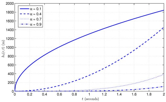
Figure 3. Hydraulic head $h_5(r,t)$ at $r=0.5\mathrm{m}$ for various fractional orders $\alpha =0.1,0.4,0.7,0.9$ in the Caputo case with $T=3.47\times {10}^{-3}{\mathrm{m}}^2/\mathrm{s}$, $S={10}^{-4}$, and $q_0={10}^{-6}\mathrm{m}/\mathrm{s}$.

Figure 4 shows the temporal variation of the approximate solution $h_5(r,t)$ at a closer radial location, $r=0.1\mathrm{m}$, for different fractional orders $\alpha =0.1,0.4,0.7,0.9$ under the Caputo framework. As expected, the hydraulic head values at this location are significantly higher than those at $r=0.5$, owing to the stronger influence of the source term $q_0{e}^{-r^2}$, which is nearly maximal at this position ($e^{-0.01}\approx 0.99$). Despite this magnitude difference, the qualitative behavior of the head profiles mirrors that observed at $r=0.5$. The curve corresponding to the lowest fractional order $\alpha =0.1$ again shows the highest head with a steep, square-root-like growth, reflecting rapid accumulation due to strong memory effects. As $\alpha$ increases, the head buildup becomes slower and more gradual, with $\alpha =0.4$ showing the next highest head, followed by $\alpha =0.7$ and then $\alpha =0.9$. This ordering reinforces the inverse relationship between fractional order and the memory depth in the Caputo model. The combination of spatial proximity to the recharge source and the nonlocal temporal memory results in intensified head responses near the origin. This further demonstrates the model’s robustness in resolving sharp hydraulic gradients near strong source zones, which is vital in applications such as managed aquifer recharge and injection-driven recovery systems.

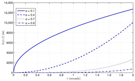
Figure 4. Hydraulic head $h_5(r,t)$ at $r=0.1\mathrm{m}$ for various fractional orders $\alpha =0.1,0.4,0.7,0.9$ in the Caputo case with $T=3.47\times {10}^{-3}{\mathrm{m}}^2/\mathrm{s}$, $S={10}^{-4}$, and $q_0={10}^{-6}\mathrm{m}/\mathrm{s}$.

Figure 5 presents the time evolution of the hydraulic head $h_5(r,t)$ at the radial location $r=0.5\mathrm{m}$, obtained using the Atangana–Baleanu–Caputo (ABC) fractional derivative for fractional orders $\alpha =0.1,0.4,0.7,0.9$. The hydraulic head increases over time due to the spatially localized exponential source $q_0{e}^{-r^2}$, which remains significantly active at this radius ($e^{-0.25}\approx 0.7788$). The temporal profiles, however, show distinct behaviors across the fractional orders. The curve for $\alpha =0.1$ exhibits a rapid initial rise, remaining above all other curves up to approximately $t=0.6$. Beyond this point, its growth slows considerably, forming a square-root-like shape and ultimately falling below the curves for higher $\alpha$ values by $t=2$, indicating the lowest hydraulic head among the considered orders at the final time. In contrast, the curves for $\alpha =0.4,0.7,0.9$ display more pronounced quadratic-like growth, with the intermediate order $\alpha =0.4$ achieving the highest final head, followed by $\alpha =0.7$, and then $\alpha =0.9$. This pattern reflects the ABC model’s memory kernel effect: smaller fractional orders induce strong early accumulation but limited long-term growth due to smoother, non-singular memory distribution, while intermediate orders balance early response with sustained accumulation. These dynamics highlight the ABC model’s nuanced capability to represent both transient sharp responses and gradual damping in hydraulic head evolution under localized recharge conditions.

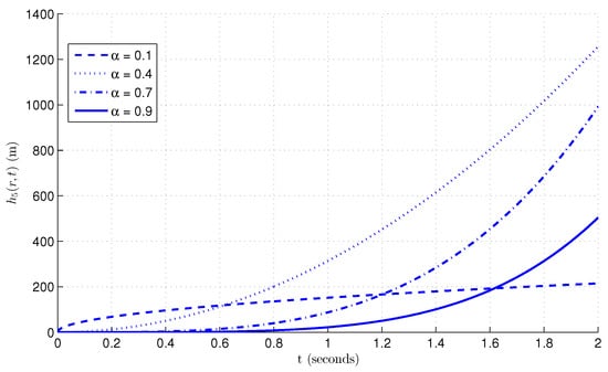
Figure 5. Hydraulic head $h_5(r,t)$ at $r=0.5\mathrm{m}$ for various fractional orders $\alpha =0.1,0.4,0.7,0.9$ in the ABC case with $T=3.47\times {10}^{-3}{\mathrm{m}}^2/\mathrm{s}$, $S={10}^{-4}$, and $q_0={10}^{-6}\mathrm{m}/\mathrm{s}$.

Figure 6 illustrates the temporal evolution of the hydraulic head $h_5(r,t)$ at the radial position $r=0.1\mathrm{m}$, located near the center of the recharge zone. Due to the exponential source term $q_0{e}^{-r^2}$, which is nearly unity at this location ($e^{-0.01}\approx 0.99$), the head values are significantly higher across all fractional orders compared to the case at $r=0.5\mathrm{m}$. The overall pattern of temporal evolution closely follows that observed at $r=0.5$. The curve for $\alpha =0.1$ initially rises rapidly and remains above the other curves up to approximately $t=0.6$. Beyond this point, its growth tapers off, forming a square-root-like trajectory, and it is eventually overtaken by the curves for higher $\alpha$ values. By $t=2$, the $\alpha =0.1$ curve results in the lowest hydraulic head among all considered fractional orders. The curves for $\alpha =0.4,0.7,0.9$ demonstrate more sustained growth with a quadratic-like shape. Among these, $\alpha =0.4$ attains the highest head at later times, followed by $\alpha =0.7$, and then $\alpha =0.9$. This behavior highlights the role of fractional memory in modulating both early and late-time responses: smaller $\alpha$ values in the ABC model facilitate rapid initial recharge accumulation, whereas moderate $\alpha$ values provide more balanced and enhanced long-term head buildup. In summary, Figure 6 illustrates the ABC model’s effectiveness in capturing spatially variable recharge effects and fractional-order memory, offering a realistic depiction of transient groundwater head dynamics in high-recharge regions.

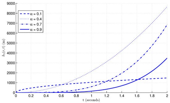
Figure 6. Hydraulic head $h_5(r,t)$ at $r=0.1\mathrm{m}$ for various fractional orders $\alpha =0.1,0.4,0.7,0.9$ in the ABC case with $T=3.47\times {10}^{-3}{\mathrm{m}}^2/\mathrm{s}$, $S={10}^{-4}$, and $q_0={10}^{-6}\mathrm{m}/\mathrm{s}$.

A comparative analysis between the Caputo and Atangana–Baleanu–Caputo (ABC) cases reveals fundamental differences in how fractional memory influences the evolution of hydraulic head over time and space. In the Caputo case, the curve corresponding to the lowest fractional order, $\alpha =0.1$, displays the most pronounced head rise across the entire time interval. The growth is rapid and sustained, consistently surpassing the head values for higher fractional orders such as $\alpha =0.4, 0.7$, and $\alpha =0.9$. This behavior highlights the singular memory kernel of the Caputo operator, which accumulates past recharge contributions without decay. As a result, the system experiences long-term amplification of the hydraulic head, particularly near the source region. Lower $\alpha$ values, therefore, reflect stronger memory effects and emphasize the influence of historical recharge events on the present state. The head profiles for $\alpha =0.4$, $\alpha =0.7$, and $\alpha =0.9$ follow a progressively subdued pattern, forming curves similar to quadratic growth, with lower overall head buildup due to weaker memory accumulation.

In contrast, the ABC case demonstrates a distinctly different temporal behavior. The curve for $\alpha =0.1$ initially rises sharply from $t=0$, dominating all other curves up to approximately $t=0.6\mathrm{s}$, and resembles a square-root-like trajectory. However, beyond this point, the growth rate diminishes considerably, and the curve is overtaken by those corresponding to higher $\alpha$ values. By $t=2\mathrm{s}$, the head for $\alpha =0.1$ becomes the lowest among all cases. The curves for $\alpha =0.4$, $0.7$, and $0.9$ show smoother and more consistent increases over time, with $\alpha =0.4$ eventually producing the highest head at late times. This inversion in trend compared to the Caputo case arises due to the non-singular and non-local memory kernel in the ABC model, which introduces exponential decay. The ABC operator allows strong early-time memory effects, followed by gradual fading, producing a tempered head evolution that is more balanced and realistic in certain hydrogeological scenarios.

A key component of the present groundwater model is the spatially localized source term $q\left(r\right)=q_0{e}^{-r^2}$, which models a recharge zone concentrated near the origin. This exponentially decaying term ensures that recharge is most intense at the center ($r\approx 0$) and gradually weakens with increasing radius. As a result, hydraulic head is highest near the center and declines outward. For instance, at $r=0.1\mathrm{m}$, the exponential factor $e^{-0.01}\approx 0.99$ allows nearly full recharge, leading to elevated head buildup. In this region, both the Caputo and ABC models demonstrate higher head values compared to $r=0.5\mathrm{m}$, with similar qualitative behavior observed between the models but at higher magnitudes due to the strong recharge influence.

As the radius increases toward the periphery ($r\ge 0.6$), the recharge term becomes negligible due to the rapid decay of $e^{-r^2}$, which approaches zero. Consequently, the hydraulic head decreases significantly and even becomes negative. This drop is attributed to the dominance of radial terms in the analytical solution (such as $H_2\left(r\right),H_3\left(r\right)$, etc.), which include large coefficients scaled by transmissivity-to-storage ratios. In these outer regions, the source is insufficient to offset outward radial flow, leading to drawdown or depletion zones. Physically, this represents a transition from recharge-dominated behavior near the center to regions experiencing net outflow or hydraulic decline.

In both the Caputo and ABC models, the spatial head distribution closely follows the profile of the source term, but the temporal response differs based on the memory formulation. The Caputo model tends to exaggerate the influence of the source due to its cumulative memory effect, resulting in steeper head gradients and more aggressive buildup near the origin. In contrast, the ABC model moderates this behavior, producing smoother transitions and more physically plausible head profiles over time and space.

Therefore, the selection of the fractional operator has a profound impact on the predicted hydraulic head response. The Caputo model is well-suited for systems with dominant historical recharge influence and long-memory persistence, while the ABC model provides a realistic framework for modeling time-fading memory effects in heterogeneous aquifers. The presence of a spatially decaying source further enhances these differences, making the choice of fractional model critical for accurately capturing the dynamics of groundwater flow in recharge-sensitive environments.

8. Conclusions

This study presented a time-fractional generalization of the classical Theis groundwater model with an exponential source, solved using the Fractional Reduced Differential Transform Method (FRDTM) under both Caputo and Atangana–Baleanu–Caputo (ABC) derivatives. The spatially localized source term allowed for realistic simulation of recharge near the origin and decreasing head outward. In the Caputo model, lower fractional orders such as $\alpha =0.1$ resulted in significant long-term head buildup due to the singular, cumulative nature of the kernel, emphasizing the dominant influence of past recharge events.

In contrast, the ABC model showed a rapid initial response at small $\alpha$, followed by early saturation and lower head at later times. Intermediate fractional orders like $\alpha =0.4$ yielded the highest long-term head due to a balance between early response and fading memory. Both models captured the spatial shift from recharge zones to depletion regions at the aquifer periphery. These results highlight that Caputo derivatives are more suitable for systems with strong memory effects, while ABC operators provide a better framework for systems with transient recharge behavior.

References

- Konikow, L.F.; Mercer, J.W. Groundwater flow and transport modeling. J. Hydrol. 1988, 100, 379–409. [Google Scholar] [CrossRef]
- Harter, T.; Zhang, D. Water flow and solute spreading in heterogeneous soils with spatially variable water content. Water Resour. Res. 1999, 35, 415–426. [Google Scholar] [CrossRef]
- Chang, C.M.; Yeh, H.D. Investigation of solute transport in nonstationary unsaturated flow fields. Hydrol. Earth Syst. Sci. 2012, 16, 4049–4055. [Google Scholar] [CrossRef]
- Bear, J. Hydraulics of Groundwater; Courier Corporation: North Chelmsford, MA, USA, 2012. [Google Scholar]
- Marsily, G.D. Quantitative Hydrogeology: Groundwater Hydrology for Engineers; Academic Press: Orlando, FL, USA, 1986. [Google Scholar]
- Knochenmus, L.A.; Robinson, J.L. Descriptions of Anisotropy and Heterogeneity and Their Effect on Ground-Water Flow and Areas of Contribution to Public Supply Wells in a Karst Carbonate Aquifer System; US Geological Survey Water-Supply Paper; U.S. Geological Survey: Reston, VA, USA, 1996.
- Hubbert, M.K. Darcy’s law and the field equations of the flow of underground fluids. Hydrol. Sci. J. 1957, 2, 23–59. [Google Scholar] [CrossRef]
- Igboekwe, M.U.; Amos-Uhegbu, C. Fundamental approach in groundwater flow and solute transport modelling using the finite difference method. Earth Environ. Sci. 2011, 556, 301–328. [Google Scholar]
- Wang, H.F.; Anderson, M.P. Introduction to Groundwater Modeling: Finite Difference and Finite Element Methods; Academic Press: Cambridge, MA, USA, 1995. [Google Scholar]
- Li, P.W.; Fan, C.M.; Chen, C.Y.; Ku, C.Y. Generalized finite difference method for numerical solutions of density-driven groundwater flows. Comput. Model. Eng. Sci. 2014, 101, 319–350. [Google Scholar]
- Chávez-Negrete, C.; Domínguez-Mota, F.J.; Román-Gutiérrez, R. Interface formulation for generalized finite difference method for solving groundwater flow. Comput. Geotech. 2024, 166, 105990. [Google Scholar] [CrossRef]
- Huyakorn, P.S.; Lester, B.H.; Faust, C.R. Finite element techniques for modeling groundwater flow in fractured aquifers. Water Resour. Res. 1983, 19, 1019–1035. [Google Scholar] [CrossRef]
- Dehghan, M.; Hooshyarfarzin, B.; Abbaszadeh, M. Numerical simulation based on a combination of finite-element method and proper orthogonal decomposition to prevent the groundwater contamination. Eng. Comput. 2022, 38 (Suppl. 4), 3445–3461. [Google Scholar] [CrossRef]
- Das, S.; Eldho, T.I. A meshless weak strong form method for the groundwater flow simulation in an unconfined aquifer. Eng. Anal. Bound. Elem. 2022, 137, 147–159. [Google Scholar] [CrossRef]
- Rajaveni, S.P.; Nair, I.S.; Brindha, K.; Elango, L. Finite element modelling to assess the submarine groundwater discharge in an over exploited multilayered coastal aquifer. Environ. Sci. Pollut. Res. 2021, 28, 67456–67471. [Google Scholar] [CrossRef] [PubMed]
- Ross, B. The development of fractional calculus. Hist. Math. 1977, 4, 75–89. [Google Scholar] [CrossRef]
- Lacroix, S.F. Traité du Calcul Différentiel et du Calcul Intégral, 2nd ed.; Courcier: Paris, France, 1819; pp. 409–410. [Google Scholar]
- Abel, N.H. Solution de quelques problèmes à l’aide d’intégrales définies. Oeuvres Complètes 1823, 1, 16–18. [Google Scholar]
- Fourier, J.B.J. Théorie analytique de la chaleur. Oeuvres Fourier 1822, 1, 508. [Google Scholar]
- Liouville, J. Mémoire sur quelques questions de géométrie et de mécanique, et sur un nouveau genre de calcul pour résoudre ces questions. J. l’École Polytech. 1832, 13, 1–69. [Google Scholar]
- Kumar, P.; Yadav, M.P.; Dubey, R.S. Dual permeability fractional model for flow in the karstic aquifer. Comput. Math. Model. 2025, 36, 139–150. [Google Scholar] [CrossRef]
- Agarwal, R.; Yadav, M.P.; Agarwal, R.P.; Goyal, R. Analytic solution of fractional advection dispersion equation with decay for contaminant transport in porous media. Matematicki Vesnik 2019, 71, 5–15. [Google Scholar]
- Agarwal, R.; Yadav, M.P.; Agarwal, R.P.; Baleanu, D. Analytic solution of space time fractional advection dispersion equation with retardation for contaminant transport in porous media. Prog. Fract. Differ. Appl. 2019, 5, 283–295. [Google Scholar]
- Agarwal, R.; Yadav, M.P.; Agarwal, R.P. Analytic solution of time fractional Boussinesq equation for groundwater flow in unconfined aquifer. J. Discontinuity Nonlinearity Complex. 2019, 8, 341–352. [Google Scholar] [CrossRef]
- Agarwal, R.; Yadav, M.P.; Agarwal, R.P. Collation analysis of fractional moisture content based model in unsaturated zone using q-homotopy analysis method. In Methods of Mathematical Modelling: Fractional Differential Equations; CRC Press: Boca Raton, FL, USA; Taylor & Francis: Abingdon, UK, 2019; p. 151. [Google Scholar]
- Agarwal, R.; Yadav, M.P.; Baleanu, D.; Purohit, S.D. Existence and uniqueness of miscible flow equation through porous media with a non singular fractional derivative. AIMS Math. 2020, 5, 1062–1073. [Google Scholar] [CrossRef]
- Maturi, D.A. Variational Iteration Method and Analytic Solution for Laplace Equation for Steady Groundwater Flow. GEOMATE J. 2024, 26, 90–97. [Google Scholar] [CrossRef]
- Yadav, M.P.; Agarwal, R. Numerical investigation of fractional-fractal Boussinesq equation. Chaos 2019, 29, 013109. [Google Scholar] [CrossRef] [PubMed]
- Monzon, G. Fractional variational iteration method for higher-order fractional differential equations. J. Fract. Calc. Appl. 2024, 15, 1–15. [Google Scholar]
- He, J.H. Approximate analytical solution for seepage flow with fractional derivatives in porous media. Comput. Methods Appl. Mech. Eng. 1998, 167, 57–68. [Google Scholar] [CrossRef]
- Kumar, P.; Yadav, M.P. Numerical approximations of groundwater flow problem using fractional variational iteration method with fractional derivative of singular and nonsingular kernel. Int. J. Math. Ind. 2024, 16, 2450008-1–2450008-15. [Google Scholar] [CrossRef]
- İbiş, B.; Bayram, M. Approximate solution of time-fractional advection-dispersion equation via fractional variational iteration method. Sci. World J. 2014, 2014, 769713. [Google Scholar] [CrossRef]
- Adomian, G. Nonlinear Stochastic Systems: Theory and Applications to Physics; Kluwer Academic Publishers: Amsterdam, The Netherlands, 1989. [Google Scholar]
- Adomian, G. Solving Frontier Problems of Physics: The Decomposition Method; Kluwer Academic Publishers: Boston, MA, USA, 1994. [Google Scholar]
- You, X.; Li, S.; Kang, L.; Cheng, L. A study of the non-linear seepage problem in porous media via the homotopy analysis method. Energies 2023, 16, 2175. [Google Scholar] [CrossRef]
- Raval, A.; Joshi, M.S. Homotopy Analysis Method for One-Dimensional Burger’s Equation in Longitudinal Dispersion Phenomena via Porous Media. Int. J. Appl. Comput. Math. 2025, 11, 144. [Google Scholar] [CrossRef]
- Raval, A.P.; Joshi, M.S. Application of Homotopy Analysis Method for Solving Fingero-Imbibition Equations in Enhanced Oil Recovery. Improv. Oil Gas Recovery 2025, 9, 1–21. [Google Scholar]
- Şengül, S.; Bekiryazici, Z.; Merdan, M. Approximate solutions of fractional differential equations using optimal q-homotopy analysis method: A case study of Abel differential equations. Fractal Fract. 2024, 8, 533. [Google Scholar] [CrossRef]
- Onyejekwe, O.N. An inverse problem for a time-fractional heat equation: Determination of a time-dependent coefficient via the Laplace homotopy analysis method. Int. J. Appl. 2025, 14, 36–39. [Google Scholar] [CrossRef]
- Morales-Delgado, V.F.; Gómez-Aguilar, J.F.; Yépez-Martínez, H.; Baleanu, D.; Escobar-Jimenez, R.F.; Olivares-Peregrino, V.H. Laplace homotopy analysis method for solving linear partial differential equations using a fractional derivative with and without kernel singularity. Adv. Differ. Equ. 2016, 2016, 164. [Google Scholar] [CrossRef]
- Srivastava, V.K.; Kumar, S.; Awasthi, M.K.; Singh, B.K. Two-dimensional time fractional-order biological population model and its analytical solution. Egypt. J. Basic Appl. Sci. 2014, 1, 71–76. [Google Scholar] [CrossRef]
- Singh, B.K. Fractional reduced differential transform method for numerical computation of a system of linear and nonlinear fractional partial differential equations. Int. J. Open Probl. Comput. Sci. Math. 2016, 9, 20–38. [Google Scholar] [CrossRef]
- Rawashdeh, M.S. A reliable method for the space-time fractional Burgers and time-fractional Cahn-Allen equations via the FRDTM. Adv. Differ. Equ. 2017, 2017, 99. [Google Scholar] [CrossRef]
- Theis, C.V. The relation between the lowering of the piezometric surface and the rate and duration of discharge of a well using ground-water storage. Trans. Am. Geophys. Union 1935, 16, 519–524. [Google Scholar] [CrossRef]
- Caputo, M. Linear models of dissipation whose Q is almost frequency independent—II. Geophys. J. Int. 1967, 13, 529–539. [Google Scholar] [CrossRef]
- Atangana, A.; Baleanu, D. New fractional derivatives with nonlocal and nonsingular kernel: Theory and application to heat transfer model. Therm. Sci. 2016, 20, 763–769. [Google Scholar] [CrossRef]
Disclaimer/Publisher’s Note: The statements, opinions and data contained in all publications are solely those of the individual author(s) and contributor(s) and not of MDPI and/or the editor(s). MDPI and/or the editor(s) disclaim responsibility for any injury to people or property resulting from any ideas, methods, instructions or products referred to in the content. |
© 2025 by the authors. Licensee MDPI, Basel, Switzerland. This article is an open access article distributed under the terms and conditions of the Creative Commons Attribution (CC BY) license (https://creativecommons.org/licenses/by/4.0/).