Fractional Differential Equations with Impulsive Effects

Abstract

This paper discusses impulsive effects on fractional differential equations. Two approaches are taken to obtain our results: either with fixed or changing lower limits in Caputo fractional derivatives. First, we derive an existence result for periodic solutions of fractional differential equations with periodically changing lower limits. Then, the impulsive effects are modeled for fractional differential equations regarding the nonlinearities rather than the initial value conditions. The proposed impulsive model differs from common discontinuous and nonsmooth dynamical systems.

1. Introduction

Fractional differential equations (FDEs) arise from engineering and scientific disciplines regarding mathematical modeling of systems in the fields of physics, aerodynamics, chemistry, electrodynamics, and so on, involving derivatives of fractional order [1,2,3,4], where the theory of impulsive differential equations (IDEs) is particularly important for its wide spectrum of applications [5,6,7]. The main reason for its applicability is due to the fact that impulsive differential problems appropriately describe many processes where, at certain moments, the states rapidly change, and these processes cannot be well modeled by classical differential equations [8,9]. Moreover, impulsive fractional differential equations (IFDEs) have found many promising applications [10,11].

Contrarily to the classical derivative, the fractional derivative is nonlocal, which leads to obstacles in studying IFDEs [12,13]. Recently, a new approach to modelling impulsive effects has been suggested and studied [14]. This approach can be used when impulses in time are non-instantaneous; that is, impulses last over certain time intervals. The present paper does not deal with this new and interesting topic of non-instantaneous IDEs; rather, it focuses on yet another way to introduce impulses into differential equations.

Now, consider a continuous mapping $f:{\mathbb{R}}_0\times {\mathbb{R}}^m\to {\mathbb{R}}^m$, where ${\mathbb{R}}_0=[0,\infty )$ and ${\left\{t_k\right\}}_{k=0}^{\infty }\subset {\mathbb{R}}_0$ is an increasing sequence so that $t_0=0$, $\underset{k\to \infty }{\lim }{t}_k=\infty$ and ${\left\{y_k\right\}}_{k=1}^{\infty }\subset {\mathbb{R}}^m$.

The objective here is to solve the following ODE:

$$x^{\prime }=f(t,x),t\in (t_k,t_{k+1})$$

(1)

with impulses

$$x\left(t_k^{+}\right)=x\left(t_k^{-}\right)+y_k.$$

(2)

A conventional approach is to start with initial value $x\left(t_0\right)=x_0$ at $t_0=0$ to solve (1) for $t\in [0,t_1)$ and apply the impulse (2) to obtain $x\left(t_1^{+}\right)=x\left(t_1^{-}\right)+y_1$, and then, we use this as the initial value to solve (1) on $[t_1,t_2)$, and so on. During this iteration process, one can use any numerical method to solve the problem on each interval $(t_k,t_{k+1})$, $k=0,1,2,\cdots$.

It follows from (1) that

$$x\left(t\right)=x\left(t_k^{+}\right)+{\int }_{t_k}^{t}f(s,x\left(s\right))ds,$$

(3)

for $t\in (t_k,t_{k+1})$, which leads to

$$\begin{array}{ccc}\hfill x\left(t\right)& =& x\left(t_k^{+}\right)+{\int }_{t_k}^{t}f(s,x\left(s\right))ds\hfill \\ & =& x\left(t_k^{-}\right)+y_k+{\int }_{t_k}^{t}f(s,x\left(s\right))ds\hfill \\ & =& x\left(t_{k-1}^{+}\right)+{\int }_{t_{k-1}}^{t_k}f(s,x\left(s\right))ds+y_k+{\int }_{t_k}^{t}f(s,x\left(s\right))ds\hfill \\ & =& x\left(t_0\right)+\sum _{i=1}^k{y}_i+\sum _{i=1}^k{\int }_{t_{i-1}}^{t_i}f(s,x\left(s\right))ds+{\int }_{t_k}^{t}f(s,x\left(s\right))ds\hfill \\ & =& x\left(t_0\right)+\sum _{i=1}^k{y}_i+{\int }_{t_0}^{t}f(s,x\left(s\right))ds\hfill \end{array}$$

for $t\in (t_0,t)$.

This approach cannot be extended to FDEs, however, keeping the lower limit at $t_0$. Note that

$$x\left(t\right)=x\left(t_0\right)+\sum _{i=1}^k{y}_i+{\displaystyle \frac{1}{\mathsf{\Gamma }\left(q\right)}}{\int }_{t_0}^t{(t-s)}^{q-1}f(s,x\left(s\right))ds,$$

(4)

for $t\in (t_0,\infty )$, is a solution to the IFDE, as presented in [13]:

$${}^{c}D_{t_0}^{q}x\left(t\right)=f(t,x),$$

(5)

for $t\in (t_0,\infty )$, with (2) and $q\in (0,1)$, fixing the lower limit at $t_0$, where ${}^{c}D_{t_0}^{q}x\left(t\right)$ is a generalized Caputo fractional derivative with lower limit at $t_0$.

Next, if the FDE version of (1) is considered in the following form:

$${}^{c}D_{t_0}^{q}x\left(t\right)=f(t,x),t\in (t_k,t_{k+1})$$

(6)

where $q\in (0,1)$, then (3) becomes

$$x\left(t\right)=x\left(t_k^{+}\right)+{\displaystyle \frac{1}{\mathsf{\Gamma }\left(q\right)}}{\int }_{t_k}^t{(t-s)}^{q-1}f(s,x\left(s\right))ds,$$

(7)

for $t\in (t_k,t_{k+1})$. Thus, one can study this type of IFDE (6) with (2) when the lower limits are changing at all impulses. Consequently, ${}^{c}D_{t_k}^{q}x\left(t\right)$ is a generalized Caputo fractional derivative with lower limit at $t_k$. Similarly, it follows from (7) that

$$\begin{array}{ccc}\hfill x\left(t\right)& =& x\left(t_k^{+}\right)+{\displaystyle \frac{1}{\mathsf{\Gamma }\left(q\right)}}{\int }_{t_k}^t{(t-s)}^{q-1}f(s,x\left(s\right))ds\hfill \\ & =& x\left(t_k^{-}\right)+y_k+{\displaystyle \frac{1}{\mathsf{\Gamma }\left(q\right)}}{\int }_{t_k}^t{(t-s)}^{q-1}f(s,x\left(s\right))ds\hfill \\ & =& x\left(t_{k-1}^{+}\right)+{\displaystyle \frac{1}{\mathsf{\Gamma }\left(q\right)}}{\int }_{t_{k-1}}^{t_k}{(t_k-s)}^{q-1}f(s,x\left(s\right))ds\hfill \\ & & +y_k+{\displaystyle \frac{1}{\mathsf{\Gamma }\left(q\right)}}{\int }_{t_k}^t{(t-s)}^{q-1}f(s,x\left(s\right))ds\hfill \\ & =& x\left(t_0\right)+\sum _{i=1}^k{y}_i+{\displaystyle \frac{1}{\mathsf{\Gamma }\left(q\right)}}\sum _{i=1}^k{\int }_{t_{i-1}}^{t_i}{(t_i-s)}^{q-1}f(s,x\left(s\right))ds\hfill \\ & & +{\displaystyle \frac{1}{\mathsf{\Gamma }\left(q\right)}}{\int }_{t_k}^t{(t-s)}^{q-1}f(s,x\left(s\right))ds\hfill \end{array}$$

for $t\in (t_k,t_{k+1})$. Because $q\in (0,1)$, there is a memory effect in (6), meaning that

$$\begin{array}{ccc}\hfill & & \sum _{i=1}^k{\int }_{t_{i-1}}^{t_i}{(t_i-s)}^{q-1}f(s,x\left(s\right))ds+{\int }_{t_k}^t{(t-s)}^{q-1}f(s,x\left(s\right))ds\hfill \\ & \ne & {\int }_{t_0}^t{(t-s)}^{q-1}f(s,x\left(s\right))ds\hfill \end{array}$$

(8)

where it is important to note that the integral kernels of the first term on the left-hand side are ${(t_i-s)}^{q-1}$ but not ${(t-s)}^{q-1}$ and that $[t_0,t)={\bigcup }_{i=0}^{k-1}[t_i,t_{i+1})\cup [t_k,t)$ holds only for $t\in (t_k,t_{k+1})$. Thus, (8) shows that the memory effect of (5) is not a sum of the memory effects of (6) on each of these subintervals.

A comparative numerical study using examples of the above two IFDEs, with fixed lower limit (5)–(2) and with changing lower limit (6), can be found in [15].

One can study two types of IFDEs: the first is (5)–(2) with a solution formula (4); the second is (6)–(2) with a solution formula (7). One can see that gluing (7) from 1 to k together does not give a solution formula (4). This is an essential difference between integer-order and fractional-order differential equations. This also implies that IFDE has no nonconstant periodic solutions when the lower limit is fixed at $t_0=0$ [16]. However, (6)–(2) may have periodic solutions when the impulses are periodic. As a matter of fact, periodic IFDEs create discrete dynamical systems, to which a general theory of difference equations can be applied [17,18].

The rest of this paper is organized as follows: Periodic IFDEs are discussed in Section 2, while other possibilities of impulsive effects on FDEs are discussed in Section 3 and Section 4, inspired by [19], wherein impulsive effects were not on the initial values but on the right-hand sides of FDEs. Finally, our conclusions and a discussion are presented in the last section.

2. Periodic IFDEs

Let ${\mathbb{N}}_0=\{0,1,2,\cdots \}$ and consider

$$\begin{array}{ccc}\hfill {}^{c}D_{t_k}^{q}x\left(t\right)& =& f(t,x\left(t\right)),t\in (t_k,t_{k+1}),k\in {\mathbb{N}}_0,\hfill \\ \hfill x\left(t_k^{+}\right)& =& x\left(t_k^{-}\right)+y_k,k\in \mathbb{N},\hfill \\ \hfill x\left(0\right)& =& x_0,\hfill \end{array}$$

(9)

where $q\in (0,1)$. Assume that

(i)

$f:{\mathbb{R}}_0\times {\mathbb{R}}^m\to {\mathbb{R}}^m$ is continuous and T-periodic in t;

(ii)

there is a constant $K\ge 0$, such that $\parallel f(t,x)-f(t,y)\parallel \le K\parallel x-y\parallel$ for all $t\in {\mathbb{R}}_0$ and $x,y\in {\mathbb{R}}^m$;

(iii)

${\left\{t_k\right\}}_{k=1}^{\infty }\subset {\mathbb{R}}_0$ is increasing, and ${\left\{y_k\right\}}_{k=1}^{\infty }\subset {\mathbb{R}}^m$, such that there is an $N\in \mathbb{N}$ with $T=t_{N+1}$, $t_{k+N+1}=t_k+T$ and $y_{k+N+1}=y_k$, for all $k\in \mathbb{N}$.

As covered in [2], under assumptions (i) and (ii), (9) has a unique solution on ${\mathbb{R}}_0$.

Now, consider the Poincaré mapping

$$P\left(x_0\right)=x\left(T^{+}\right).$$

Clearly, the fixed points of P determine the T-periodic solutions of (9) ([20], Lemma 2.2). The following existence and uniqueness result follows ([21], Lemma 2.1 and Theorem 2.2).

Theorem 1.

Under assumptions (i) and (ii), it holds that

$$\parallel P\left(x\right)-P\left(y\right)\parallel \le \mathsf{\Theta }\parallel x-y\parallel ,\forall x,y\in {\mathbb{R}}^m$$

with

$$\mathsf{\Theta }=\prod _{k=0}^N{E}_q\left(K{(t_{k+1}-t_k)}^q\right),$$

(10)

where $t_0=0$, and $E_q$ is the Mittag–Leffler function (see ([2], p. 40)). If (iii) holds as well and $\mathsf{\Theta }<1$, then (9) has a unique T-periodic solution ${\overline{x}}_0\in {\mathbb{R}}^m$, which is asymptotically stable, namely

$$\parallel {\overline{x}}_0-P^n\left(y_0\right)\parallel \le {\mathsf{\Theta }}^n\parallel {\overline{x}}_0-y_0\parallel$$

for all $n\in \mathbb{N}$ and $y_0\in {\mathbb{R}}^m$.

To this end, the following existence can be established.

Theorem 2.

Suppose that assumptions (i) and (iii) hold, and moreover,

(iv) 

there are constants $K\ge 0$ and $L\ge 0$, such that $\parallel f(t,x)\parallel \le K\parallel x\parallel +L$ for all $t\in {\mathbb{R}}_0$ and $x\in {\mathbb{R}}^m$.

If $\mathsf{\Theta }<1$ in (10), then (9) has a T-periodic solution ${\overline{x}}_0\in {\mathbb{R}}^m$, satisfying

$$\begin{array}{ccc}\hfill \parallel {\overline{x}}_0\parallel \le r_0& =& {\displaystyle \frac{1}{1-\mathsf{\Theta }}}(\sum _{k=0}^N\prod _{j=N-k}^N{E}_q\left(K{(t_{j+1}-t_j)}^q\right)\hfill \\ & & \times \left(\parallel y_{N-k+1}\parallel +{\displaystyle \frac{{(t_{N-k+1}-t_{N-k})}^q}{\mathsf{\Gamma }(q+1)}}\right)).\hfill \end{array}$$

(11)

Proof. 

On each interval $(t_k,t_{k+1})$, $k=0,1,\cdots ,N$, Equation (9) is equivalent to

$$x\left(t\right)=x\left(t_k^{+}\right)+{\displaystyle \frac{1}{\mathsf{\Gamma }\left(q\right)}}{\int }_{t_k}^t{(t-s)}^{q-1}f(s,x\left(s\right))ds.$$

This implies that

$$\begin{array}{ccc}\hfill \parallel x\left(t\right)\parallel & \le & \parallel x\left(t_k^{+}\right)\parallel +{\displaystyle \frac{1}{\mathsf{\Gamma }\left(q\right)}}{\int }_{t_k}^t{(t-s)}^{q-1}\parallel f(s,x\left(s\right))\parallel ds\hfill \\ & \le & \parallel x\left(t_k^{+}\right)\parallel +{\displaystyle \frac{1}{\mathsf{\Gamma }\left(q\right)}}{\int }_{t_k}^t{(t-s)}^{q-1}(K\parallel x\left(s\right)\parallel + L)ds\hfill \\ & =& \parallel x\left(t_k^{+}\right)\parallel +{\displaystyle \frac{L{(t-t_k)}^q}{\mathsf{\Gamma }(q+1)}}+{\displaystyle \frac{K}{\mathsf{\Gamma }\left(q\right)}}{\int }_{t_k}^t{(t-s)}^{q-1}\parallel x\left(s\right)\parallel ds.\hfill \end{array}$$

(12)

Applying the Gronwall fractional inequality ([3], Theorem 1) to (12) leads to

$$\parallel x\left(t\right)\parallel \le \left(\parallel x\left(t_k^{+}\right)\parallel +{\displaystyle \frac{L{(t-t_k)}^q}{\mathsf{\Gamma }(q+1)}}\right)E_q\left(K{(t-t_k)}^q\right),t\in (t_k,t_{k+1}),$$

which gives

$$\begin{array}{ccc}\hfill \parallel x\left(t_{k+1}^{+}\right)\parallel & \le & \left(\parallel y_{k+1}\parallel +{\displaystyle \frac{L{(t_{k+1}-t_k)}^q}{\mathsf{\Gamma }(q+1)}}\right)E_q\left(K{(t_{k+1}-t_k)}^q\right)\hfill \\ & & +E_q\left(K{(t_{k+1}-t_k)}^q\right)\parallel x\left(t_k^{+}\right)\parallel \hfill \end{array}$$

for $k=0,1,\cdots ,N$. Consequently,

$$\begin{array}{ccc}\hfill \parallel P\left(x_0\right)\parallel & =& \parallel x\left(t_{N+1}^{+}\right)\parallel \le \sum _{k=0}^N\prod _{j=N-k}^N{E}_q\left(K{(t_{j+1}-t_j)}^q\right)\hfill \\ & & \times \left(\parallel y_{N-k+1}\parallel +{\displaystyle \frac{{(t_{N-k+1}-t_{N-k})}^q}{\mathsf{\Gamma }(q+1)}}\right)+\mathsf{\Theta }\parallel x_0\parallel .\hfill \end{array}$$

If $\parallel x_0\parallel \le r_0$, then (11) implies $\parallel P\left(x_0\right)\parallel \le r_0$. Hence, P has a fixed point in the ball $B_{r_0}\left(0\right)$ by the Brouwer fixed point theorem. The proof is complete. □

Remark 1.

Clearly, $\left(ii\right)\Rightarrow \left(iv\right)$, but $\left(iv\right)\nRightarrow \left(ii\right)$. Hence, (iv) does not guarantee the uniqueness of solutions.

From the above discussion, it follows that

$$\begin{array}{ccc}\hfill {}^{c}D_0^{q}x\left(t\right)& =& f(t,x\left(t\right)),t\in (t_k,t_{k+1}),k\in {\mathbb{N}}_0,\hfill \\ \hfill x\left(t_k^{+}\right)& =& x\left(t_k^{-}\right)+y_k,k\in \mathbb{N},\hfill \\ \hfill x\left(0\right)& =& x_0\hfill \end{array}$$

has no periodic solutions. So, it suffices to consider only the periodic condition

$$x\left(T\right)=x\left(0\right).$$

More related results can be found in [21].

Example 1.

Consider the simplest case of a linear FDE with a period-one impulse sequence, described by

$$\begin{array}{ccc}\hfill {}^{c}D_k^{q}x\left(t\right)& =& Ax\left(t\right),t\in (k,k+1),k\in {\mathbb{N}}_0,\hfill \\ \hfill x\left(k^{+}\right)& =& x\left(k^{-}\right)+y,k\in \mathbb{N},\hfill \\ \hfill x\left(0\right)& =& x_0,\hfill \end{array}$$

(13)

where $q\in (0,1)$ and A is an $m\times m$ matrix, with

$$P\left(x_0\right)=x\left(1^{+}\right)=E_q\left(A\right)x_0+y.$$

(14)

A fixed point $x_0$ of (14) is determined by

$$(I-E_q\left(A\right))x_0=y,$$

which is uniquely solvable, and

$$x_0={(I-E_q\left(A\right))}^{-1}=y$$

if and only if $1\notin \sigma \left(E_q\left(A\right)\right)$.

If $1\in \sigma \left(E_q\left(A\right)\right)$, then the Lyapunov–Schmidt method [22] can be applied. Specifically, for the case of $m=3$ and $Ax=x\times v$ with a vector product × and $v=(0,0,\eta )$, where $\eta \in \mathbb{R}$, one has

$$\begin{array}{ccc}\hfill {}^{c}D_k^{q}x\left(t\right)& =& x\left(t\right)\times v,t\in (k,k+1),k\in {\mathbb{N}}_0,\hfill \\ \hfill x\left(k^{+}\right)& =& x\left(k^{-}\right)+y,k\in \mathbb{N},\hfill \\ \hfill x\left(0\right)& =& x_0.\hfill \end{array}$$

(15)

Note that

$$(x_1,x_2,x_3)\times v=\eta (-x_2,x_1,0).$$

Thus,

$$A=\left(\begin{array}{ccc}0& -\eta & 0\\ \eta & 0& 0\\ 0& 0& 0\end{array}\right).$$

(16)

Setting $z=x_1+x_2ı$, where $ı=\sqrt{-1}$, and identifying ${\mathbb{R}}^3$ with $\mathbb{C}\times \mathbb{R}$, i.e., $(x_1,x_2,x_3)=(z,u)$, one obtains

$$(z,u)\times v=(\eta ız,0).$$

Then, (15) is transformed to

$$\begin{array}{ccc}\hfill {}^{c}D_k^{q}z\left(t\right)& =& \eta ız, {}^{c}D_k^{q}u\left(t\right)=0,t\in (k,k+1),k\in {\mathbb{N}}_0,\hfill \\ \hfill z\left(k^{+}\right)& =& z\left(k^{-}\right)+y_1,u\left(k^{+}\right)=u\left(k^{-}\right)+y_2,k\in \mathbb{N},\hfill \\ \hfill z\left(0\right)& =& z_0,u\left(0\right)=u_0\hfill \end{array}$$

(17)

for $y=(y_1,y_2)\in \mathbb{C}\times \mathbb{R}$. Thus, (14) becomes

$$P(z_0,u_0)=(E_q(\eta ı)z_0+y_1,u_0+y_2).$$

(18)

Since $E_q(\eta ı)$ is a complex number, the only fixed point of (18) is

$$z_0=\left({\displaystyle \frac{y_1}{1-E_q(\eta ı)}},u_0\right)$$

which exists only if $y_2=0$.

Note that, for the matrix A defined in (16), $\sigma \left(A\right)=\{\pm \eta ı,0\}$.

Now, consider a small perturbation $\epsilon \in \mathbb{R}$ to (17), yielding

$$\begin{array}{ccc}\hfill {}^{c}D_k^{q}z\left(t\right)& =& \eta ız\left(t\right)+\epsilon u\left(t\right)z\left(t\right),{}^{c}D_k^{q}u\left(t\right)=\epsilon u\left(t\right)\Re z\left(t\right),t\in (k,k+1),k\in {\mathbb{N}}_0,\hfill \\ \hfill z\left(k^{+}\right)& =& z\left(k^{-}\right)+y_1,u\left(k^{+}\right)=u\left(k^{-}\right)+\epsilon y_2,k\in \mathbb{N},\hfill \\ \hfill z\left(0\right)& =& z_0,u\left(0\right)=u_0\hfill \end{array}$$

(19)

Then, in (19) expanding

$$z\left(t\right)=z_0\left(t\right)+\epsilon z_1\left(t\right)+O\left({\epsilon }^2\right),u\left(t\right)=u_0\left(t\right)+\epsilon u_1\left(t\right)+O\left({\epsilon }^2\right),$$

yields

$$\begin{array}{ccc}\hfill {}^{c}D_k^q{z}_0\left(t\right)& =& \eta ız_0\left(t\right),{}^{c}D_k^q{u}_0\left(t\right)=0,t\in (k,k+1),k\in {\mathbb{N}}_0,\hfill \\ \hfill z_0\left(k^{+}\right)& =& z_0\left(k^{-}\right)+y_1,u_0\left(k^{+}\right)=u_0\left(k^{-}\right),k\in \mathbb{N},\hfill \\ \hfill z_0\left(0\right)& =& z_0,u_0\left(0\right)=u_0\hfill \end{array}$$

(20)

and

$$\begin{array}{ccc}\hfill {}^{c}D_k^q{z}_1\left(t\right)& =& \eta ız_1\left(t\right)+u_0\left(t\right)z_0\left(t\right),{}^{c}D_k^q{u}_1\left(t\right)=u_0\left(t\right)\Re \left(z_0\left(t\right)\right),t\in (k,k+1),k\in {\mathbb{N}}_0,\hfill \\ \hfill z_1\left(k^{+}\right)& =& z_1\left(k^{-}\right),u_1\left(k^{+}\right)=u_1\left(k^{-}\right)+y_2,k\in \mathbb{N},\hfill \\ \hfill z\left(0\right)& =& 0,u\left(0\right)=0.\hfill \end{array}$$

(21)

Thus, (20) and (21) together give

$$\begin{array}{ccc}\hfill z_0\left(t\right)& =& E_q(\eta t^qı)z_0,u_0\left(t\right)=u_0,\hfill \\ \hfill z_1\left(t\right)& =& u_0{z}_0{\int }_0^t{(t-s)}^{q-1}{E}_{q,q}\left(\eta {(t-s)}^q\right)E_q(\eta s^qı)ds,\hfill \\ \hfill u_1\left(t\right)& =& {\displaystyle \frac{u_0}{\mathsf{\Gamma }\left(q\right)}}{\int }_0^t{(t-s)}^{q-1}\Re \left(E_q(\eta s^qı)z_0\right)ds\hfill \end{array}$$

for $t\in [0,1)$. Consequently, (14) becomes

$$\begin{array}{ccc}\hfill P(z_0,u_0)& =& (z_0\left(1^{-}\right)+\epsilon z_1\left(1^{-}\right)+y_1+O\left({\epsilon }^2\right),u_0\left(1^{-}\right)+\epsilon u_1\left(1^{-}\right)+\epsilon y_2+O\left({\epsilon }^2\right))\hfill \\ & =& (\left(E_q(\eta ı)+\epsilon u_0{\int }_0^1{(1-s)}^{q-1}{E}_{q,q}\left(\eta {(1-s)}^q\right)E_q(\eta s^qı)ds\right)z_0+y_1,\hfill \\ & & \left(1+\epsilon {\displaystyle \frac{1}{\mathsf{\Gamma }\left(q\right)}}{\int }_0^1{(1-s)}^{q-1}\Re \left(E_q(\eta s^qı)z_0\right)ds\right)u_0+\epsilon y_2)+O\left({\epsilon }^2\right).\hfill \end{array}$$

(22)

A fixed point of (22) is given by

$$\begin{array}{ccc}\hfill z_0& =& \left(E_q(\eta ı)+\epsilon u_0{\int }_0^1{(1-s)}^{q-1}{E}_{q,q}\left(\eta {(1-s)}^q\right)E_q(\eta s^qı)ds\right)z_0+y_1+O\left({\epsilon }^2\right),\hfill \\ \hfill u_0& =& \left(1+\epsilon {\displaystyle \frac{1}{\mathsf{\Gamma }\left(q\right)}}{\int }_0^1{(1-s)}^{q-1}\Re \left(E_q(\eta s^qı)z_0\right)ds\right)u_0+\epsilon y_2+O\left({\epsilon }^2\right).\hfill \end{array}$$

(23)

Solving the first equation of (23) gives

$$\begin{array}{ccc}\hfill z_0& =& {\displaystyle \frac{1}{1-E_q(\eta ı)}}\left(\epsilon u_0{\int }_0^1{(1-s)}^{q-1}{E}_{q,q}\left(\eta {(1-s)}^q\right)E_q(\eta s^qı)ds\right)z_0\hfill \\ & & +{\displaystyle \frac{y_1}{1-E_q(\eta ı)}}+O\left({\epsilon }^2\right)={\displaystyle \frac{y_1}{1-E_q(\eta ı)}}\hfill \\ & & +\epsilon {\displaystyle \frac{y_1}{{(1-E_q(\eta ı))}^2}}{u}_0{\int }_0^1{(1-s)}^{q-1}{E}_{q,q}\left(\eta {(1-s)}^q\right)E_q(\eta s^qı)ds+O\left({\epsilon }^2\right).\hfill \end{array}$$

(24)

It follows from the second equation of (23) with (24) that

$$\begin{array}{ccc}\hfill 0& =& {\displaystyle \frac{1}{\mathsf{\Gamma }\left(q\right)}}{\int }_0^1{(1-s)}^{q-1}\Re \left(E_q(\eta s^qı)z_0\right)ds{u}_0+y_2+O\left(\epsilon \right)\hfill \\ & =& {\displaystyle \frac{u_0}{\mathsf{\Gamma }\left(q\right)}}{\int }_0^1{(1-s)}^{q-1}\Re \left({\displaystyle \frac{y_1{E}_q(\eta s^qı)}{1-E_q(\eta ı)}}\right)ds+y_2+O\left(\epsilon \right).\hfill \end{array}$$

(25)

If

$${\int }_0^1{(1-s)}^{q-1}\Re \left({\displaystyle \frac{y_1{E}_q(\eta s^qı)}{1-E_q(\eta ı)}}\right)ds\ne 0,$$

(26)

then (25) gives

$$u_0=-{\displaystyle \frac{y_2\mathsf{\Gamma }\left(q\right)}{{\int }_0^1{(1-s)}^{q-1}\Re \left(\frac{y_1{E}_q(\eta s^qı)}{1-E_q(\eta ı)}\right)ds}}+O\left(\epsilon \right).$$

(27)

Finally, inserting (27) into (24) leads to

$$z_0={\displaystyle \frac{y_1}{1-E_q(\eta ı)}}-\epsilon {\displaystyle \frac{y_1{y}_2\mathsf{\Gamma }\left(q\right){\int }_0^1{(1-s)}^{q-1}{E}_{q,q}\left(\eta {(1-s)}^q\right)E_q(\eta s^qı)ds}{{(1-E_q(\eta ı))}^2{\int }_0^1{(1-s)}^{q-1}\Re \left(\frac{y_1{E}_q(\eta s^qı)}{1-E_q(\eta ı)}\right)ds}}+O\left({\epsilon }^2\right).$$

(28)

In summary, the following result is obtained.

Theorem 3.

Assuming (26), for any small $\epsilon \in \mathbb{R}$, IFDE (19) has a fixed point given by (27) and (28).

To this end, one can take specific values of q, η, ε, $y_2$ and $y_1$ in Theorem 3 to numerically study the dynamics of (18), which will not be further discussed here.

3. Weighted FDEs

Now, consider the case where the impulsive effects are not on the initial values but on the right-hand side of the FDEs.

Specifically, consider $t_k=k$ and take ${\left\{{\eta }_k\right\}}_{k\in {\mathbb{N}}_0}\subset {\mathbb{R}}_0$. Motivated by [19], introduce the following FDE:

$${}^{c}D_0^{q}x\left(t\right)=f(t,x\left(t\right),{(1-\left\{t\right\})}^{{\eta }_{\left[x\right(t\left)\right]}}x\left(t\right)),t\in {\mathbb{R}}_0,x\left(0\right)=x_0,$$

where $\left\{t\right\}=t-\left[t\right]$ is the fractional part of t.

Example 2.

Consider

$${}^{c}D_0^{q}x=ax+b{(1-\left\{t\right\})}^{{\eta }_{\left[x\right]}}x+c{x}^3+d\cos t,$$

(29)

which gives

$$\begin{array}{ccc}\hfill x\left(t\right)& =& x\left(0\right)+{\displaystyle \frac{1}{\mathsf{\Gamma }\left(q\right)}}\sum _{j=0}^{k-1}{\int }_j^{j+1}{(t-s)}^{q-1}(ax\left(s\right)+b{(1+j-s)}^{{\eta }_j}x\left(s\right)+c{x}^3\left(s\right)+d\cos s)ds\hfill \\ & & +{\displaystyle \frac{1}{\mathsf{\Gamma }\left(q\right)}}{\int }_k^t{(t-s)}^{q-1}(ax\left(s\right)+b{(1+k-s)}^{\eta }+c{x}^3\left(s\right)+d\cos s)ds.\hfill \end{array}$$

The solvability of (29) can be studied either by applying fixed point theorems or by numerical methods, which will not be further discussed here.

4. More General FDEs with Impulsive Effects

Consider another situation where the impulsive effects are not on the initial values but on the right-hand sides of the FDEs.

Let $q\in (0,1]$ and take an increasing sequence $P={\left\{p_k\right\}}_{k=0}^{\infty }$ with $p_0=0$ and ${\lim }_{k\to \infty }{p}_k=\infty$. Consider

$${}^{c}D_0^{q}x\left(t\right)=f(t,x\left(t\right),x\left(p_{\lfloor t\rfloor }\right)),t\in {\mathbb{R}}_0,x\left(0\right)=x_0,$$

(30)

where $\lfloor ·\rfloor$ is an induced floor function given by

$$\lfloor t\rfloor =k,t\in [p_k,p_{k+1}).$$

Thus, (30) can be rewritten as

$${}^{c}D_0^{q}x\left(t\right)=f(t,x\left(t\right),x\left(p_k\right)),t\in [p_k,p_{k+1}).$$

Consequently, (30) has “impulses” at the nonlinearity but not at the argument t. This is a kind of impulsive delay differential equation. The solution of (30) is given by

$$x\left(t\right)=x\left(0\right)+{\displaystyle \frac{1}{\mathsf{\Gamma }\left(q\right)}}{\int }_0^t{(t-s)}^{q-1}f(s,x\left(s\right),x\left(p_{\lfloor s\rfloor }\right))ds.$$

(31)

Now, add control parameters ${\left\{y_k\right\}}_{k=0}^{\infty }\subset \mathbb{R}$, ${\left\{z_k\right\}}_{k=0}^{\infty }\subset \mathbb{R}$ and modify (30) to obtain the following:

$${}^{c}D_0^{q}x\left(t\right)=f(t,x\left(t\right),y_{\lfloor t\rfloor }x\left(p_{\lfloor t\rfloor }\right)+z_{\lfloor t\rfloor }),x\left(0\right)=x_0.$$

(32)

Thus, (32) becomes

$${}^{c}D_0^{q}x\left(t\right)=f(t,x\left(t\right),y_{k}x\left(p_k\right)+z_k),t\in [p_k,p_{k+1}),$$

which gives

$$x\left(t\right)=x\left(0\right)+{\displaystyle \frac{1}{\mathsf{\Gamma }\left(q\right)}}{\int }_0^t{(t-s)}^{q-1}f(s,x\left(s\right),y_{\lfloor s\rfloor }x\left(p_{\lfloor s\rfloor }\right)+z_{\lfloor s\rfloor })ds.$$

(33)

A simple form of (32) is

$${}^{c}D_0^{q}x\left(t\right)=f(t,x\left(t\right))+y_{\lfloor t\rfloor }x\left(p_{\lfloor t\rfloor }\right)+z_{\lfloor t\rfloor },x\left(0\right)=x_0,$$

(34)

where the unperturbed part is given by

$${}^{c}D_0^{q}x\left(t\right)=f(t,x\left(t\right)),x\left(0\right)=x_0.$$

(35)

One may consider controlling the solutions of (35) with (34), which can be written as

$${}^{c}D_0^{q}x\left(t\right)=f(t,x\left(t\right))+y_{k}x\left(p_k\right)+z_k,t\in [p_k,p_{k+1}),x\left(0\right)=x_0.$$

Furthermore, one may consider a weighted control problem:

$${}^{c}D_0^{q}x\left(t\right)=f(t,x\left(t\right))+y_{\lfloor t\rfloor }x\left(p_{\lfloor t\rfloor }\right)e^{-\alpha (t-p_{\lfloor t\rfloor })}+z_{\lfloor t\rfloor }{e}^{-\beta (t-p_{\lfloor t\rfloor })},x\left(0\right)=x_0,$$

(36)

namely,

$${}^{c}D_0^{q}x\left(t\right)=f(t,x\left(t\right))+y_{k}x\left(p_k\right)e^{-\alpha (t-p_k)}+z_k{e}^{-\beta (t-p_k)},t\in [p_k,p_{k+1}),x\left(0\right)=x_0$$

for $\alpha ,\beta \in {\mathbb{R}}_0$.

Finally, one may consider a more general form of (30), such as

$${}^{c}D_0^{q}x\left(t\right)=f(t,x\left(t\right),x\left(p_{\lfloor t\rfloor }\right),x\left(p_{\lfloor t\rfloor -1}\right)),x\left(0\right)=x_0,$$

(37)

and extend the ideas described above, from (30) to (37).

Remark 2.

If $P={\mathbb{N}}_0$, i.e., $p_k=k$ with $k\in {\mathbb{N}}_0$, then $p_{\lfloor t\rfloor }=\lfloor t\rfloor$ for the standard floor function $\lfloor ·\rfloor$. This kind of equation is studied in [19] for a scalar case and for integer-order derivatives.

The simplest case of (30) is its linear version

$${}^{c}D_0^{q}x\left(t\right)=Ax\left(t\right)+Bx\left(p_{\lfloor t\rfloor }\right)+g\left(t\right),t\in {\mathbb{R}}_0,x\left(0\right)=x_0$$

(38)

with $n\times n$ matrices $A,B\in M\left(n\right)$ and $g\in C({\mathbb{R}}_0,{\mathbb{R}}^n)$. The homogeneous case

$${}^{c}D_0^{q}x\left(t\right)=Ax\left(t\right)+Bx\left(p_{\lfloor t\rfloor }\right),t\in {\mathbb{R}}_0,x\left(0\right)=x_0$$

(39)

defines a linear problem. This means that (39) has a fundamental matrix solution $X\left(t\right)\in M\left(n\right)$ that solves

$${}^{c}D_0^{q}X\left(t\right)=AX\left(t\right)+BX\left(p_{\lfloor t\rfloor }\right),t\in {\mathbb{R}}_0,X\left(0\right)=I.$$

(40)

Therefore, the solution of (39) is $x\left(t\right)=X\left(t\right)x_0$, $t\in {\mathbb{R}}_0$. A semilinear case is

$${}^{c}D_0^{q}x\left(t\right)=Ax\left(t\right)+Bx\left(p_{\lfloor t\rfloor }\right)+g(t,x\left(t\right)),t\in {\mathbb{R}}_0,x\left(0\right)=x_0$$

(41)

with $g\in C({\mathbb{R}}_0\times {\mathbb{R}}^n,{\mathbb{R}}^n)$.

Example 3.

Consider $P={\mathbb{N}}_0$ and a scalar case of (41):

$${}^{c}D_0^{q}x\left(t\right)=ax\left(t\right)+bx\left(\lfloor t\rfloor \right)+c{x}^3\left(t\right)+d\cos t.$$

(42)

By (31), one has

$$\begin{array}{ccc}\hfill x\left(t\right)& =& x\left(0\right)+{\displaystyle \frac{1}{\mathsf{\Gamma }\left(q\right)}}{\int }_0^t{(t-s)}^{q-1}(ax\left(s\right)+bx\left(\lfloor s\rfloor \right)+c{x}^3\left(s\right)+d\cos s)ds\hfill \\ & =& x\left(0\right)+{\displaystyle \frac{1}{\mathsf{\Gamma }\left(q\right)}}{\int }_0^t{(t-s)}^{q-1}(ax\left(s\right)+c{x}^3\left(s\right)+d\cos s)ds\hfill \\ & & +{\displaystyle \frac{b}{\mathsf{\Gamma }\left(q\right)}}\sum _{j=0}^{k-1}x\left(j\right){\int }_j^{j+1}{(t-s)}^{q-1}ds+{\displaystyle \frac{b}{\mathsf{\Gamma }\left(q\right)}}x\left(k\right){\int }_k^t{(t-s)}^{q-1}ds\hfill \\ & =& x\left(0\right)+{\displaystyle \frac{1}{\mathsf{\Gamma }\left(q\right)}}{\int }_0^t{(t-s)}^{q-1}(ax\left(s\right)+c{x}^3\left(s\right)+d\cos s)ds\hfill \\ & & +b\sum _{j=0}^{k-1}x\left(j\right){\displaystyle \frac{{(t-j)}^q-{(t-j-1)}^q}{\mathsf{\Gamma }(q+1)}}+bx\left(k\right){\displaystyle \frac{{(t-k)}^q}{\mathsf{\Gamma }(q+1)}}.\hfill \end{array}$$

(43)

for $t\in [k,k+1)$.

Note that (43) implies that

$$\begin{array}{ccc}\hfill x(k+1)& =& x\left(0\right)+{\displaystyle \frac{1}{\mathsf{\Gamma }\left(q\right)}}{\int }_0^{k+1}{(k+1-s)}^{q-1}(ax\left(s\right)+c{x}^3\left(s\right)+d\cos s)ds\hfill \\ & & +b\sum _{j=0}^{k-1}x\left(j\right){\displaystyle \frac{{(k+1-j)}^q-{(k-j)}^q}{\mathsf{\Gamma }(q+1)}}+{\displaystyle \frac{bx\left(k\right)}{\mathsf{\Gamma }(q+1)}},\hfill \end{array}$$

(44)

which gives a recurrent formula for computing the $x\left(j\right)$ in (43). One may perform a numerical simulation of (42) for certain values of $q,a,b,c,d$, which will not be further discussed here.

The influence of the impulsive delay in (42) can be studied by introducing its weight dependence, which is as follows:

$${}^{c}D_0^{q}x\left(t\right)=ax\left(t\right)+b{e}^{-\eta \left\{t\right\}}x\left(\lfloor t\rfloor \right)+c{x}^3\left(t\right)+d\cos t,$$

where $\eta \in {\mathbb{R}}_0$ and $\left\{t\right\}=t-(\lfloor t\rfloor )$ is the fractional part of t. Thus, (43) becomes

$$\begin{array}{ccc}\hfill x\left(t\right)& =& x\left(0\right)+{\displaystyle \frac{1}{\mathsf{\Gamma }\left(q\right)}}\sum _{j=0}^{k-1}{\int }_j^{j+1}{(t-s)}^{q-1}(ax\left(s\right)+b{e}^{-\eta (s-j)}x\left(j\right)+c{x}^3\left(s\right)+d\cos s)ds\hfill \\ & & +{\displaystyle \frac{1}{\mathsf{\Gamma }\left(q\right)}}{\int }_k^t{(t-s)}^{q-1}(ax\left(s\right)+b{e}^{-\eta (s-k)}x\left(k\right)+c{x}^3\left(s\right)+d\cos s)ds.\hfill \end{array}$$

Consequently, the larger the η, the more $x\left(j\right)$ is concentrated near j.

Example 4.

Motivated by the above example, but with non-fixed lower limits in Caputo derivatives, consider

$${}^{c}D_k^{q}x\left(t\right)=ax\left(t\right)+b{e}^{-\eta (k+1-t)}x{\left(k\right)}^p,t\in [k,k+1),k\in {\mathbb{N}}_0,p\in \{1,2\}.$$

(45)

This gives

$$x\left(t\right)=E_q\left(a{(t-k)}^q\right)x\left(k\right)+bx{\left(k\right)}^p{\int }_k^t{E}_{q,q}\left(a{(t-s)}^q\right)e^{-\eta (k+1-s)}ds,$$

where $E_q$ and $E_{q,q}$ are Mittag–Leffler functions, which implies that

$$\begin{array}{ccc}\hfill x(k+1)& =& E_q\left(a\right)x\left(k\right)+bx{\left(k\right)}^p{\int }_k^{k+1}{E}_{q,q}\left(a{(k+1-s)}^q\right)e^{-\eta (k+1-s)}ds\hfill \\ & =& E_q\left(a\right)x\left(k\right)+bx{\left(k\right)}^p{\int }_0^1{E}_{q,q}\left(a{s}^q\right)e^{-\eta s}ds.\hfill \end{array}$$

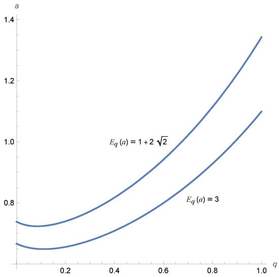
The dynamics of ${\left\{x\left(k\right)\right\}}_{k\in {\mathbb{N}}_0}$ are presented by a function

$$F\left(x\right)=E_q\left(a\right)x\left(k\right)(1-\widehat{b}x{\left(k\right)}^{p-1}),\widehat{b}=-b{\displaystyle \frac{{\int }_0^1{E}_{q,q}\left(a{s}^q\right)e^{-\eta s}ds}{E_q\left(a\right)}}.$$

(46)

When $p=1$, (46) is a linear map, and it is stable for

$$E_q\left(a\right)|1-\widehat{b}|\le 1.$$

When $p=2$, (46) is the well-known logistic map [17,23] with complex dynamics. The equation

$$E_q\left(a\right)=3$$

(47)

characterizes a border between simple and non-simple dynamics—the period-doubling bifurcation—as shown by Figure 1.

Figure 1. The curves of (47) and (48).

Note that the equation

$$E_q\left(a\right)=1+2\sqrt{2}$$

(48)

characterizes a border between non-simple and chaotic dynamics. A period-three cycle emerges, and system (45) is chaotic in the sense of Li–Yorke chaos for every $a\ge E_q^{-1}(1+2\sqrt{2})$, as shown by Figure 1.

5. Conclusions and Discussion

Ordinary differential equations (ODEs) play a crucial role in modelling evolutional processes with orbits depending continuously on time. When orbits have discontinuities in time for certain values, ODEs with impulses are used, forming the impulsive ODEs (IODEs). Another extension of ODEs is to generalize their integer derivatives to noninteger ones, which leads to fractional calculus and fractional differential equations (FDEs), which have been well developed [2,5,6,8,9]. The next natural development is the combination of the theories of IODEs and FDEs to create a new research direction of impulsive FDEs (IFDEs) [13]. This paper proposes some new forms of modelling impulsive effects in FDEs. Usually, impulses are presented in the time evolution of solutions. Here, impulsive effects are not imposed on initial values but on the right-hand sides of FDEs. The proposed impulsive models differ from the common discontinuous and nonsmooth dynamical systems in many aspects, as discussed in [24,25]. Clearly, a combination of different impulses can be an interesting topic to study. Hopefully, the ideas presented here could contribute to the further development of impulsive evolution equations. Note that other types of impulsive models exist. This is another good topic for future research. For example, changing the lower limit at $t_k$ instead of $t_0$ opens up the opportunity to use this kind of IFDE in various applications (see, e.g., [15]).

References

- Atkinson, C.; Osseiran, A. Rational solutions for the time-fractional diffusion equation. SIAM J. Appl. Math. 2011, 71, 92–106. [Google Scholar] [CrossRef]
- Kilbas, A.A.; Srivastava, H.M.; Trujillo, J.J. Theory and Applications of Fractional Differential Equations; Elsevier Science B.V.: Amsterdam, The Netherlands, 2006. [Google Scholar]
- Ye, H.; Gao, J.; Ding, Y. A generalized Gronwall inequality and its application to a fractional differential equation. J. Math. Anal. Appl. 2007, 328, 1075–1081. [Google Scholar] [CrossRef]
- Benchohra, M.; Bouriah, S.; Salim, A.; Zhou, Y. Fractional Differential Equations: A Coincidence Degree Approach; Walter de Gruyter GmbH & Co KG: Berlin, Germany; Boston, MA, USA, 2023. [Google Scholar]
- Bainov, D.D.; Simeonov, P.S. Impulsive Differential Equations: Periodic Solutions and Applications; CRC Press: Boca Raton, FL, USA, 1993. [Google Scholar]
- Samoilenko, A.M.; Perestyuk, N.A. Impulsive Differential Equations; World Scientific: Singapore, 1995. [Google Scholar]
- Liu, X.; Ballinger, G. Boundedness for impulsive delay differential equations and applications to population growth models. Nonlinear Anal. Theory Methods Appl. 2003, 53, 1041–1062. [Google Scholar] [CrossRef]
- Chicone, C. Ordinary Differential Equations with Applications, 2nd ed.; Springer Science+Bussiness Media, Inc.: New York, NY, USA, 2006. [Google Scholar]
- Teschl, G. Ordinary Differential Equations and Dynamical Systems; American Mathematical Society: Providence, RI, USA, 2010. [Google Scholar]
- Stamov, T.; Stamov, G.; Stamova, I. Fractional-order impulsive delayed reaction-diffusion gene regulatory networks: Almost periodic solutions. Fractal Fract. 2023, 7, 384. [Google Scholar] [CrossRef]
- Wang, Q.; Lu, D.; Fang, Y. Stability analysis of impulsive fractional differential systems with delay. Appl. Math. Lett. 2015, 40, 1–6. [Google Scholar] [CrossRef]
- Abbas, S.; Benchohra, M.; Nieto, J.J. Caputo-Fabrizio fractional differential equations with instantaneous impulses. AIMS Math. 2021, 6, 2932–2946. [Google Scholar] [CrossRef]
- Wang, J.R.; Fečkan, M.; Zhou, Y. On the concept and existence of solution for impulsive fractional differential equations. Commun. Nonlinear Sci. Numer. Simulations 2012, 17, 3050–3060. [Google Scholar] [CrossRef]
- Wang, J.R.; Fečkan, M. Non-Instantaneous Impulsive Differential Equations, Basic Theory and Computation; IOP Publishing Ltd.: Bristol, UK, 2018. [Google Scholar]
- Danca, M.-F.; Fečkan, M. Memory principle of the Matlab code for Lyapunov exponents of fractional order. Int. J. Bifurc. Chaos, 2024, accepted. [CrossRef]
- Kaslik, E.; Sivasundaram, S. Non-existence of periodic solutions in fractional-order dynamical systems and a remarkable difference between integer and fractional-order derivatives of periodic functions. Nonlinear Anal. Real World Appl. 2012, 13, 1489–1497. [Google Scholar] [CrossRef]
- Elaydi, S.N. An Introduction to Difference Equations, 3rd ed.; Springer Science+Business Media, Inc.: New York, NY, USA, 2005. [Google Scholar]
- Irwin, M.C. Smooth Dynamical Systems; Academic Press: London, UK, 1980. [Google Scholar]
- Cooke, K.L.; Wiener, J. Retarded differential equations with piecewise constant delays. J. Math. Anal. Appl. 1984, 99, 265–297. [Google Scholar] [CrossRef]
- Fečkan, M.; Wang, J.R.; Zhou, Y. Periodic solutions for nonlinear evolution equations with non-instantaneous impulses. Nonautonomous Dyn. Sys. 2014, 1, 93–101. [Google Scholar]
- Fečkan, M.; Wang, J.R. Periodic impulsive fractional differential equations. Adv. Nonlinear Anal. 2019, 8, 482–496. [Google Scholar] [CrossRef]
- Deimling, K. Nonlinear Functional Analysis; Springer: Berlin/Heidelberg, Germany, 1985. [Google Scholar]
- Smítal, J. On Functions and Functional Equations; Adam Hilger: Bristol, UK, 1988. [Google Scholar]
- di Bernardo, M. Piecewise-Smooth Dynamical Systems: Theory and Applications; Springer: London, UK, 2008. [Google Scholar]
- Filippov, A.F. Differential Equations with Discontinuous Right-Hand Sides; Kluwer Academic: Dordrecht, The Netherlands, 1988. [Google Scholar]
Disclaimer/Publisher’s Note: The statements, opinions and data contained in all publications are solely those of the individual author(s) and contributor(s) and not of MDPI and/or the editor(s). MDPI and/or the editor(s) disclaim responsibility for any injury to people or property resulting from any ideas, methods, instructions or products referred to in the content. |
© 2024 by the authors. Licensee MDPI, Basel, Switzerland. This article is an open access article distributed under the terms and conditions of the Creative Commons Attribution (CC BY) license (https://creativecommons.org/licenses/by/4.0/).