A Rapid Method to Quantify High-Frequency-Dominant Signals Based on Fixed-Interval Fractal Dimension

Abstract

The fractal dimension (FD) is an effective indicator to characterize various signals in engineering. However, the FD is nearly twice that of its maximum value when examining high-frequency-dominant signals, such as those in milling chatter. Previous studies in the literature have generally employed signal-pre-processing methods that require a significant amount of time to lower the FD range, thus enabling the distinguishment of different states while disabling online monitoring. A new quantitative method based on the FD within a fixed interval was constructed in this study to address this issue. First, the relationship between the fixed-interval fractal dimension (FFD) and the energy ratio (ER), named the fractal complexity curve (FC-Curve), was established, and the sensitivity region of the FFD was determined. Second, a high-frequency suppression filter (HSF) with a high calculation speed was proposed to suppress the signal’s ER so the FFD could be adjusted within its sensitivity region. Moreover, a fast energy ratio (FER) correlated with the FFD was proposed using the FC-Curve and HSF to quantitatively analyze dominant high-frequency signals. Finally, the proposed method was verified via its application in milling chatter identification. The FER method accomplished signal analysis more quickly than the traditional energy ratio difference and entropy methods, demonstrating its feasibility for online monitoring and chatter suppression in practical engineering applications.

1. Introduction

The fractal dimension (FD) evaluates the complexity [1] of a fractal curve and characterizes the frequency-domain distribution in the time domain. The signal becomes more complex as the FD increases. The FD is advantageous for biological signal analysis [2,3,4,5], wear and aging monitoring [6,7], voice signals [8,9], etc. The “complexity” is mainly characterized by the time domain curves of the Weierstrass–Mandelbrot (WM) functions [10,11,12], with FD = 1~2. Some curves lack fractal features, such as extremely smooth surfaces, characterized by WM functions at an FD of <1. Li et al. [12] pointed out that the roughness scaling extraction (RSE) method can analyze smooth non-fractal curves. Many digital signals with a significant variance in engineering are also non-fractal. After hardware acquisition, physical phenomena may lose their fractal characteristics due to the loss of high-frequency information. For example, when the main normalized frequency component is greater than 0.5, the detailed information is lost because the multiplicative frequency exceeds the hardware bandwidth. Such signals are called high-frequency-dominant signals and are approximated by WM functions with an FD of >2. Many signals in engineering lack fractal characteristics, like fractal signals, whose FDs are between one and two. Fractal and non-fractal signals thus have similar FDs but different frequency characteristics. The FD of non-fractalized signals does not reflect self-similarity, so it loses its mathematical properties. However, applications have shown that the FD can characterize the frequency domain. A new evaluation system is proposed in this study to clarify the relationship between the FD and frequency features.

Furthermore, there is a lack of guidance on interval selection when calculating the fractal dimension. Jamshidi et al. empirically determined the computational intervals in identifying bearing wear faults [13] and tool wear [6]. However, this interval selection cannot be applied to other areas. A fixed-interval fractal dimension (FFD) based on the conventional fractal dimension was proposed to address this issue. A fractal complexity curve (FC-Curve) was constructed based on the relationship between the FFD and the signal energy ratio (ER). In this study, the ER is defined as the ratio of high-frequency energy to low-frequency energy.

A problem with the FD in engineering applications is the inability to analyze signals with an excessive ER. The FD has good applicability for two types of signals, including smaller ER signals such as microseismic monitoring events [14], bioelectrical signals [2,3,4,5,15], wear and aging signals [6,7,16], and so on. Additionally, the ER differs between different signals, such as heartbeat signals [17], cough signals [18], and short-circuit fault signals [19]. However, the FD cannot distinguish between two states with a large ER, such as in milling chatter detection [20] and extracting fatigue driving from voice signals [8]. The FD almost loses its distinguishing ability when beyond the sensitivity range, e.g., fluctuating at around two. To solve this problem, most scholars have adopted signal denoising or signal reconstruction methods. Ji et al. [21,22] reconstructed a signal from key sub-signals after decomposition and then calculated its FD to identify the milling chatter. Zhuo et al. [23] carried out wavelet denoising and then identified the milling chatter of thin-walled blades via the FD. Sharma et al. [14] applied an analytic time–frequency flexible wavelet transform to filter EEG signals and calculate the FD to identify epilepsy. Smooth multi-scale morphological filtering [24] improves the FD’s capabilities by individually filtering at different scales. In addition, a low-pass filter or bandpass filter [5,14,25] can effectively reduce noise. However, it is unsuitable for signals with a wide frequency-domain distribution. In this study, a high-frequency suppression filter (HSF) is proposed, designed to suppress high-frequency energy and the ER within the FD’s sensitivity range, providing a new option to expand the FD’s applicability.

A milling chatter signal is a typical high-frequency-dominated signal. Therefore, milling chatter identification was used to verify the applicability of the HSF and FC-Curve. Machining chatter is a strong self-excited vibration phenomenon that can lead to problems such as poor machining surface quality and rapid tool wear. Chatter can be detected and avoided by monitoring the machining process. The transition from stability to chattering can occur rapidly, so high-efficiency real-time methods are needed. Most current frequency-domain methods have problems with a low computational efficiency and long time windows, e.g., modal decomposition [26,27,28,29], time–frequency features [30,31], and wavelet decomposition [32,33]. Liu et al. [27] decomposed the signal with variational modal decomposition (VMD) and then calculated the energy entropy to identify chatter. Wang et al. [29] decomposed the milling signals of thin-walled workpieces by VMD, calculated multi-scale permutation entropy, and finally discriminated the chattering by a support vector machine. Hao et al. [32] proposed a novel chatter detection method based on multi-source signals fusion using wavelet packet decomposition (WPD) and power entropy. Zhang et al. [34] optimized the computational efficiency of variational modal decomposition (VMD), and the calculation time was 59 ms~310 ms with 2500 data (500 ms). However, it still cannot be used for online monitoring. Most frequency-domain methods cannot realize real-time monitoring. Meanwhile, the FD is a time domain method, which is more suitable for online analysis due to having a short time window and high computational efficiency. However, the current FD has the following problems:

• The FD of non-fractal signals does not match the mathematical definition of a fractal. Hence, a new non-fractal evaluation system is required.
• Guidance is lacking on the interval selection for FD calculation when analyzing non-fractal signals.
• The FD tends toward two and loses resolution when analyzing non-fractal signals with a large ER.

This study proposes a fast energy ratio (FER) method suitable for online chatter monitoring based on the FC-Curve and HSF. ${\mathrm{FER}}_{\mathrm{h}\mathrm{i}\mathrm{g}\mathrm{u}\mathrm{c}\mathrm{h}\mathrm{i}}$ takes 21 μs to compute 192 data.

2. Theoretical Method

This paper does not propose a new fractal method, but rather optimizes the traditional fractal method by giving calculation intervals and designing HSF.

2.1. Fractal Signal and Non-Fractal Signal

Firstly, the characteristics of fractal and non-fractal signals are clarified. The WM function [10,11,12] describes the ideal fractal signals as follows.

$$z\left(x\right)=G^{\mathrm{FD}-1}\sum _{n_{\mathrm{m}\mathrm{i}\mathrm{n}}}^{n_{\mathrm{m}\mathrm{a}\mathrm{x}}}{\gamma }^{\left(\mathrm{FD}-2\right)n}\left(\mathit{cos}{\phi }_n-\mathit{cos}\left({\gamma }^{n}x+{\phi }_n\right)\right)$$

(1)

where $z\left(x\right)$ is the signal amplitude at the time distance x, $G$ is the characteristic length scale, and ${\gamma }^n$ is the discrete frequency spectrum of the signal; normally $\gamma =1.5$. $n_{\mathrm{m}\mathrm{i}\mathrm{n}}$ and $n_{\mathrm{m}\mathrm{a}\mathrm{x}}$ are the cut-off frequency. ${\phi }_n$ is the random phase. From the ideal fractal signal equation, the amplitude $A$ and frequency $f$ are related as follows.

$$A_n={\gamma }^{\mathrm{FD}-2}{A}_{n-1}$$

(2)

$$f_n=f_{n-1}/\gamma$$

(3)

Thus, as $f$ increases by a factor $\gamma$, $A$ decreases by a factor ${\gamma }^{\mathrm{FD}-2}$. The ideal fractal case is shown in Figure 1a. As the high-frequency energy gradually increases, the limiting case ($\mathrm{FD}\approx 2$) shown in Figure 1b occurs. When increased further, the curve no longer has a fractal character ($\mathrm{FD}>2$), as shown in Figure 1d. Digital signals will generally not satisfy Equation (3). A signal that satisfies Equation (2) but not Equation (3) is called an approximate non-fractal, as shown in Figure 1c. Signals with approximate fractal features can be applied to fractal analysis methods.

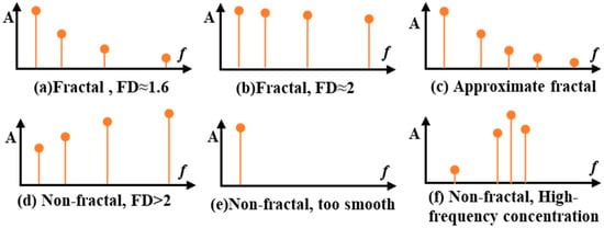
Figure 1. Typical spectral distribution characteristics of fractal and non-fractal signals.

But there are a lot of non-fractal signals in engineering. Figure 1e depicts the over-smooth retarded non-fractal signal, analysed by Li et al. [12]. When choosing an economical sampling frequency, the signal is approximately as shown in Figure 1f. If it does not satisfy Equations (2) and (3), traditional fractal analysis cannot be applied to this situation.

2.2. Properties of Fractal Characteristic Curves

The RSE fractal dimension (${\mathrm{FD}}_{\mathrm{R}\mathrm{S}\mathrm{E}}$) [34] is determined based on roughness, which helps us to understand the fractal characteristic curves. The Higuchi fractal dimension (${\mathrm{FD}}_{\mathrm{h}\mathrm{i}\mathrm{g}\mathrm{u}\mathrm{c}\mathrm{h}\mathrm{i}}$) [35] is better suited for real-time monitoring scenarios due to its computational efficiency. This study mainly discusses and analyzes the ${\mathrm{FD}}_{\mathrm{R}\mathrm{S}\mathrm{E}}$ and ${\mathrm{FD}}_{\mathrm{h}\mathrm{i}\mathrm{g}\mathrm{u}\mathrm{c}\mathrm{h}\mathrm{i}}$. The conclusions can be generalized to other fractal methods.

The RSE method calculates the FD via an Rq−Len curve. The Rq−Len curve under 0th-order flattening is calculated as follows: Let $X$ be a sequence with $N$ data points. $X$ is decomposed into $M$ subsequences $x_i$ with similar intervals and length $Len$. $i=\mathrm{1,2},\cdots ,M$. $Len$ is the scale. The $SubR{q}_i$ value for each subinterval $x_i$ is calculated as follows.

$$SubR{q}_i=\sqrt{{\displaystyle \frac{1}{Len}}\sum _{j=1}^{Len}{\left(x_{ij}-{\stackrel{\text{-}}{x}}_i\right)}^2},{\stackrel{\text{-}}{x}}_i={\displaystyle \frac{1}{Len}}\sum _{j=1}^{Len}{x}_j$$

(4)

${\stackrel{\text{-}}{x}}_i$ represents the average value of the $i$-th subsequence, $j$ represents the subinterval number, and $SubR{q}_i$ is the $Rq$ of the subsequences. The $Rq$ under the signal scale $Len$ is calculated as follows.

$$Rq\left(Len\right)={\displaystyle \frac{1}{M}}\sum _{i=1}^{M}SubR{q}_i$$

(5)

The Rq−Len curve is obtained by plotting $Rq$ and $Len$ in a logarithmic coordinate system. ${\mathrm{FD}}_{\mathrm{R}\mathrm{S}\mathrm{E}}$ is calculated as follows.

$${\mathrm{FD}}_{\mathrm{R}\mathrm{S}\mathrm{E}}=2-k_{\mathrm{Rq}}$$

(6)

where $k_{\mathrm{Rq}}$ is the slope of the Rq−Len curve. Zhang et al. [36] showed that the Rq−Len curve has linear interval segments in a logarithmic coordinate system when the data series possesses fractal characteristics.

The Higuchi method calculates the FD via the 1/k−L(k) curve [35]. Let $X$ be a sequence with $N$ data points. $L\left(1\right),L\left(2\right),\cdots ,L\left(k_{max}\right)$ is generated via $k_{max}$, where $1\le {k⌈N/2⌉}_{max}$ $⌈*⌉$ indicates upward rounding. $L\left(k\right)$ is calculated as follows.

$$L_m\left(k\right)={\displaystyle \frac{1}{k}}{\displaystyle \frac{N-1}{⌈\frac{N-m}{k}⌉k}}\sum _{i=1}^{⌈{\displaystyle \frac{N-m}{k}}⌉}\left|X\left(m+ik\right)-X\left(m+\left(i-1\right)k\right)\right|$$

(7)

$$L(k)={\displaystyle \frac{1}{k}}\sum _{m=1}^k{L}_m\left(k\right)$$

(8)

Higuchi’s fractal characteristic curve is obtained by plotting $\left(1/k,L\left(k\right)\right)$ in a logarithmic coordinate system.

$${\mathrm{FD}}_{\mathrm{h}\mathrm{i}\mathrm{g}\mathrm{u}\mathrm{c}\mathrm{h}\mathrm{i}}=k_L$$

(9)

where $k_L$ is the slope of the 1/k−L(k) curve. The properties were analyzed based on analog signals to better understand the fractal dimension. Several analog signals with a sampling frequency of 25,600 Hz were selected as follows, all with an energy sum of 2.

$$\begin{array}{l}Sig1=\sqrt{2}\mathit{cos}\left(80\pi t\right)\\ Sig2=\mathit{cos}\left(80\pi t\right)+\mathit{cos}\left(800\pi t\right)\\ \begin{array}{l}Sig3=\mathit{cos}\left(80\pi t\right)+\sqrt{0.7}\mathit{cos}\left(800\pi t\right)+\sqrt{0.3}\mathit{cos}\left(8000\pi t\right)\\ Sig4=\sqrt{1.7}\mathit{cos}\left(80\pi t\right)+\sqrt{0.3}\mathit{cos}\left(800\pi t\right)\end{array}\end{array}$$

(10)

Figure 2a approximately marks three blue dashed lines parallel to the y-axis based on the corner positions with $Len$ scales of 6, 64, and 640. The horizontal coordinates are divided into four regions, R1~R4. The corner is located at the intersection of the Rq−Len curve with the vertical dashed line. The frequency component is associated with the corner. Figure 2b shows a similar phenomenon. The frequency and scale correspond with each other, as shown below.

$$f\left(Len\right)=Fs/Len; f\left(k\right)=Fs/k$$

(11)

where $f$ is the frequency of the signal component, $Fs$ is the sampling frequency, and Len and k are the scale.

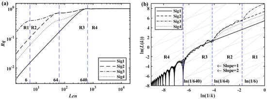
Figure 2. (a) Rq−Len curve, (b) 1/k−L(k) curve.

The slopes of the four curves are approximately the same in the R1 region in Figure 2a. The slope decreases whenever the energy increases. After $Len=640$, all the frequency components are included and the slopes in the R4 region are all zero. For Sig1, no new components appear in any of the three regions R1~R3, so its slope stays close to 1. For Sig2 and Sig3, the energy ratios are the same, so they overlap in the R3 region. For Sig2 and Sig4, Sig4 has a lower energy ratio, so the slope is smaller. The slope near Len in the Rq−Len curve reflects the $\mathrm{ER}$. The fractal dimension increases as the high-frequency energy increases. The newly added frequency component $f\left(Le{n}_0\right)$ in the Rq−Len curve affects the regions larger than $Le{n}_0$ without affecting regions smaller than $Le{n}_0$. Figure 2b shows a similar, but not sufficiently significant, trend.

2.3. FFD and Fractal Complexity Curve

The spectrum of an actual signal becomes denser and contains more frequency components as the scale increases. Therefore, there would not be an ideal linear interval as in Figure 2. The energy ratio is defined herein.

$$\mathrm{ER}=\sum f_{\mathrm{High}}^2/\sum f_{\mathrm{Low}}^2$$

(12)

where $F_e$ is the estimation frequency and $Fs$ is the sampling frequency. $f_{\mathrm{High}}$ is the high-frequency component of the spectrum ($F_e<f_{\mathrm{High}}<Fs/2$). Similarly, $f_{\mathrm{Low}}$ is the low-frequency component of the spectrum. When analyzing signal complexity, the low-frequency components close to the direct current component are, generally, eliminated. The low-frequency components close to the direct current are not included in the $\mathrm{ER}$ defined in this study, so $0.0025Fs<f_{\mathrm{Low}}<F_e$. The signal complexity described by the $\mathrm{FFD}$ reflects the $\mathrm{ER}$. The larger the $\mathrm{ER}$, the larger the $\mathrm{FFD}$.

The $\mathrm{FFD}$ pertaining to the RSE and Higuchi is defined as follows. The estimation region ($R$) contains the scales used to calculate the $\mathrm{FFD}$. According to Equation (11), $Le{n}_{\mathrm{e}}$ or $k_{\mathrm{e}}$ is the estimation scale, and the corresponding frequency is the estimation frequency ($F_{\mathrm{e}}$). As shown in Figure 2, the RSE method is more stable, so $R$ only needs to define the interval endpoints (e.g., $R=\left[\mathrm{8,12}\right]$). For ${\mathrm{FFD}}_{\mathrm{R}\mathrm{S}\mathrm{E}}$, $Len$ cannot be too small when calculating $Rq$, so the fixed intervals of the RSE are chosen as follows.

$$Le{n}_{\mathrm{e}}=\left(Le{n}_{\mathrm{m}\mathrm{a}\mathrm{x}}+Le{n}_{\mathrm{m}\mathrm{i}\mathrm{n}}\right)/2; Le{n}_{\mathrm{m}\mathrm{i}\mathrm{n}}\ge 8$$

(13)

where $Le{n}_{\mathrm{m}\mathrm{i}\mathrm{n}}~Le{n}_{\mathrm{m}\mathrm{a}\mathrm{x}}$ are the scale ranges of the fixed intervals. $Le{n}_{\mathrm{e}}$ is the estimate scale. The ${\mathrm{FFD}}_{\mathrm{R}\mathrm{S}\mathrm{E}}$ is calculated by Equation (6). The optimal number of subintervals is 140, and the optimal signal length is 192 data.

Higuchi’s characteristic curve is more unstable, so the calculation needs all the scales and the ${\mathrm{FFD}}_{\mathrm{H}\mathrm{i}\mathrm{g}\mathrm{u}\mathrm{c}\mathrm{h}\mathrm{i}}$ value is obtained via linear fitting (e.g., $R=1~12$). The best signal length is also 192 data, and the fixed intervals of the Higuchi are chosen as follows.

$$k_{\mathrm{e}}=\left(k_{\mathrm{m}\mathrm{a}\mathrm{x}}+k_{\mathrm{m}\mathrm{i}\mathrm{n}}+7\right)/2; k_{min}=1$$

(14)

where $k_{\mathrm{m}\mathrm{i}\mathrm{n}}~k_{\mathrm{m}\mathrm{a}\mathrm{x}}$ are the scale ranges of the fixed intervals. $k_{\mathrm{e}}$ is the estimate scale. The ${\mathrm{FFD}}_{\mathrm{H}\mathrm{i}\mathrm{g}\mathrm{u}\mathrm{c}\mathrm{h}\mathrm{i}}$ is calculated by Equation (9).

To summarize, the calculations of FFD and FD are the same, except that the FFD used the intervals specified in Equations (13) and (14). Therefore, the qualitative analysis of FFD in the latter section applies equally to FD. The relationship between the $\mathrm{FFD}$ and $\mathrm{ER}$ was explored via simulation signals. The simulation signals can adjust the $\mathrm{ER}$, which has a randomized composition, phase, and amplitude.

$$\begin{array}{c}Si{g}_{\mathrm{Low}}={\displaystyle \sum _{i=1}^N}{B}_i\mathit{cos}\left(2\pi f_{\mathrm{Low}}\left(i\right)t+{\phi }_i\right)\\ Si{g}_{\mathrm{High}}={\displaystyle \sum _{j=1}^M}{C}_j\mathit{cos}\left(2\pi f_{\mathrm{High}}\left(j\right)t+{\varphi }_j\right)\\ Sig=Si{g}_{\mathrm{Low}}+K\times Si{g}_{\mathrm{High}}\\ K=\sqrt{ER{\displaystyle \sum _{i=1}^N}{f}_{\mathrm{Low}}^2(i)/{\displaystyle \sum _{i=1}^M}{f}_{\mathrm{High}}^2(i)}\end{array}$$

(15)

$B_i,C_j,randN,randM$ is a random number within [0, 1]. $N=⌈15+20\times randN⌉$ is the number of $f_{\mathrm{Low}}$, and $M=⌈40+20\times randM⌉$ is the number of $f_{\mathrm{High}}$. ${\phi }_i$ and ${\varphi }_j$ are the random phases within [0, 2π]. $\mathrm{ER}=\mathrm{0.01,0.02},\cdots ,20$ was selected for simulation. Figure 3 shows the 2000 simulation results for $\mathrm{ER}=2$, which approximately conform to a normal distribution. Each $\mathrm{ER}$ was calculated 2000 times and fitted to obtain the mean $\mu$ and variance $\sigma$. $\sigma$ resulted from the different phases of the frequency component and was not a computational error.

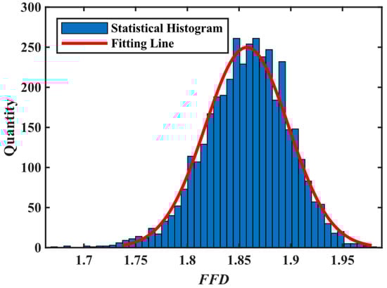
Figure 3. When $\mathrm{ER}=2$, the statistical results of calculating $\mathrm{FD}$ values 2000 times, and an approximately normal distribution fitting was used, resulting in a good fitting result.

Based on the fixed interval parameters in Figure 4, Figure 5, Figure 6, Figure 7 and Figure 8 and Equations (4)–(9), the results of $\mu$ and $\sigma$ were calculated according to Figure 3, and their characteristics were analyzed later on. The $\mu$ and $\sigma$ characteristic curves in Figure 4 highly overlap, proving that the specified ${\mathrm{FFD}}_{\mathrm{R}\mathrm{S}\mathrm{E}}$ can evaluate the corresponding $\mathrm{ER}$. The characteristic curves in Figure 4a are not close to overlapping because $F_e$ is a constant value. This means that there is a definite relationship between the FFD (calculated from Equations (13) and (14)) and ER. The curve in Figure 4a is named the FC-Curve in this paper, taking the following form.

$${\mathrm{FFD}}_{\mathrm{FC}\text{-}\mathrm{Curve}}\left(\mathrm{ER}\right)=a{e}^{-0.75\mathrm{ER}}+b{e}^{-4.5\mathrm{ER}}+c{\mathrm{ER}}^{0.1}+d$$

(16)

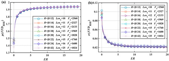
Figure 4. Energy ratio characteristic curve of ${\mathrm{FFD}}_{\mathrm{R}\mathrm{S}\mathrm{E}}$ generates signals with $F_{\mathrm{e}}=Fs/{Len}_{\mathrm{e}}$: (a) the mean value $\mu$ curves are similar. This curve is called Fractal Complexity Curve. When $\mathrm{ER}>7$, μ increases slowly; (b) the variances $\sigma$ are also similar, when $\mathrm{ER}>5$, $\sigma$ is close to 0.022.

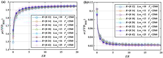
Figure 5. Energy ratio characteristic curve of ${\mathrm{FFD}}_{\mathrm{R}\mathrm{S}\mathrm{E}}$, and generate signals with $F_{\mathrm{e}}=2560 \mathrm{H}\mathrm{z}$: (a) $\mu$ curves do not coincide. (b) $\sigma$ curves also do not coincide.

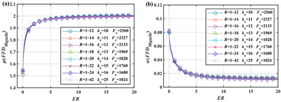
Figure 6. Energy ratio characteristic curve of ${\mathrm{FFD}}_{\mathrm{H}\mathrm{i}\mathrm{g}\mathrm{u}\mathrm{c}\mathrm{h}\mathrm{i}}$, and generate signals with $F_{\mathrm{e}}=Fs/{Len}_{\mathrm{e}}$. The results are like Figure 4: (a) the mean value $\mu$ curves are similar; (b) the variances $\sigma$ are also similar. When $\mathrm{ER}>5$, $\sigma <0.015$.

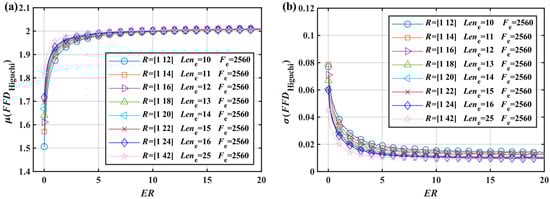
Figure 7. Energy ratio characteristic curve of ${\mathrm{FFD}}_{\mathrm{H}\mathrm{i}\mathrm{g}\mathrm{u}\mathrm{c}\mathrm{h}\mathrm{i}}$, and generate signals with $F_{\mathrm{e}}=2560 \mathrm{H}\mathrm{z}$: (a) $\mu$ curves do not coincide. (b) $\sigma$ curves also do not coincide.

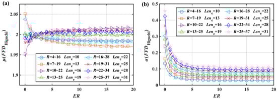
Figure 8. Energy ratio characteristic curve of ${\mathrm{FFD}}_{\mathrm{H}\mathrm{i}\mathrm{g}\mathrm{u}\mathrm{c}\mathrm{h}\mathrm{i}}$, and generate signals with the start length change: (a) When start length is too large, ${\mathrm{FFD}}_{\mathrm{H}\mathrm{i}\mathrm{g}\mathrm{u}\mathrm{c}\mathrm{h}\mathrm{i}}$ probably decreases with the increase in $\mathrm{ER}$; this is not normal and is unpredictable; (b) the variances $\sigma$ are small, too.

The FC-Curve’s coefficients after ${\mathrm{FFD}}_{\mathrm{R}\mathrm{S}\mathrm{E}}$ fitting were $a=-0.1709; b=-0.2055; c=0.1588; d=1.728$ (linear fitting-adjusted $R^2=0.9995$; expected fit).

The $\mu$ and $\sigma$ characteristic curves in Figure 6 also highly overlap and those in Figure 7 do not. Therefore, the ${\mathrm{FFD}}_{\mathrm{H}\mathrm{i}\mathrm{g}\mathrm{u}\mathrm{c}\mathrm{h}\mathrm{i}}$ also had an FC-Curve, and the fitting coefficients were $a=-0.1446; b=-0.2269; c=0.1286; d=1.827$ (linear fitting-adjusted $R^2=0.9994$). For ${\mathrm{FFD}}_{\mathrm{R}\mathrm{S}\mathrm{E}}$ and ${\mathrm{FFD}}_{\mathrm{H}\mathrm{i}\mathrm{g}\mathrm{u}\mathrm{c}\mathrm{h}\mathrm{i}}$, the analysis shows that the FC-Curve was a property of the $\mathrm{FFD}$. As shown in Figure 8a, some fixed intervals led to the anomaly of the ${\mathrm{FFD}}_{\mathrm{H}\mathrm{i}\mathrm{g}\mathrm{u}\mathrm{c}\mathrm{h}\mathrm{i}}$ decreasing as the $\mathrm{ER}$ increased. This means that the calculation interval cannot be chosen arbitrarily.

Most fractal studies are based on the WM function. As such, the applicability of the FC-Curve was verified with the WM function [10,11] ($\gamma =1.5$; $Fs=\mathrm{25,600} \mathrm{Hz}$; $n_{\mathrm{L}}=11(f_{\mathrm{L}}=86 \mathrm{Hz})$; $n_{\mathrm{e}}=19(F_{\mathrm{e}}=2216 \mathrm{Hz})$; and $n_{\mathrm{H}}=+\infty$). When $\mathrm{FD}>2$, $n_H$ was appropriately reduced ($E_{\mathrm{L}}={{\sum }_{m=n_L}^{n_{\mathrm{e}}}\left({\displaystyle \frac{1}{{\gamma }^{\left(2-\mathrm{FD}\right)m}}}\right)}^2$; $E_{\mathrm{H}}={{\sum }_{m=n_{\mathrm{e}}}^{+\infty }\left({\displaystyle \frac{1}{{\gamma }^{\left(2-\mathrm{FD}\right)m}}}\right)}^2$; and $\mathrm{ER}=E_{\mathrm{H}}/E_{\mathrm{L}}$). The $\mathrm{FD}$ was predicted according to Equation (16). The results are shown in Table 1.

Table 1. Generate WM functions with FD and make predictions about FD via FC-Curve.

WM Function		FC-Curve
$\mathbf{FD}$	$\mathbf{ER}$	$\overline{{\mathit{F}\mathit{F}\mathit{D}}_{\mathbf{R}\mathbf{S}\mathbf{E}}}$	Error_$\overline{{\mathit{F}\mathit{F}\mathit{D}}_{\mathbf{R}\mathbf{S}\mathbf{E}}}$	$\overline{{\mathit{F}\mathit{F}\mathit{D}}_{\mathbf{H}\mathbf{i}\mathbf{g}\mathbf{u}\mathbf{c}\mathbf{h}\mathbf{i}}}$	Error_$\overline{{\mathit{F}\mathit{F}\mathit{D}}_{\mathbf{Higuchi}}}$
1.5	0.061	1.53	1.90%	1.56	7.57%
1.6	0.011	1.57	1.63%	1.61	3.75%
1.7	0.212	1.64	3.57%	1.69	1.57%
1.8	0.442	1.72	4.25%	1.77	0.59%
1.9	1.187	1.81	4.29%	1.87	0.14%
1.93	1.818	1.85	3.95%	1.927	0.14%
1.96	3.486	1.90	3.30%	1.962	0.11%
1.98	7.261	1.92	2.99%	1.983	0.16%
2.3	72	1.97	/	2.02	/

$\overline{{FFD}_{\mathrm{H}\mathrm{i}\mathrm{g}\mathrm{u}\mathrm{c}\mathrm{h}\mathrm{i}}}$ and $\overline{{FFD}_{\mathrm{R}\mathrm{S}\mathrm{E}}}$ resulted from using the FC-Curve to predict the $\mathrm{FD}$ value via the $\mathrm{ER}$. The prediction of $\overline{{FFD}_{\mathrm{H}\mathrm{i}\mathrm{g}\mathrm{u}\mathrm{c}\mathrm{h}\mathrm{i}}}$ improved with an increasing $\mathrm{FD}$. The analysis demonstrated that the FC-Curve can establish an estimate between the $\mathrm{FD}$ and $\mathrm{ER}$.

The $\mathrm{ER}$ of the fractal signal represented by the WM function is generally not more than 3. However, the signal $\mathrm{ER}$ in engineering is much larger, e.g., the ER of milling chatter signals may reach 300, and the traditional FD calculation method cannot analyze this kind of signal. The FC-Curve was used to calculate the FFD and unify the frequency-domain characteristics of fractal and non-fractal signals in this study. The signal $\mathrm{ER}$ can be estimated by calculating the $\mathrm{FFD}$. Li et al. [37] refined the analysis of oversimplified non-fractal signals, filling this gap in the research.

2.4. Sensitivity Range of FFD

The ${\mathrm{FFD}}_{\mathrm{R}\mathrm{S}\mathrm{E}}$ was used as an example to analyze the FFD’s capability range. The interval was $R=\left[\mathrm{8,12}\right] ({Len}_{\mathrm{e}}=10)$. Consider $\mathrm{ER}$ and $\mathrm{FFD}$ as independent continuous random variables. Consider $\left(\mathrm{ER},\mathrm{FFD}\right)$ as a two-dimensional continuous random variable with joint probability density $f\left(\mathrm{ER},\mathrm{FFD}\right)$. The marginal probability density of the $\left(\mathrm{ER},\mathrm{FFD}\right)$ at $\mathrm{ER}=e{r}_i$ was plotted based on the FC-Curve and $\sigma$ curves in Figure 9b. All marginal probability densities in the ER-FFD coordinate system were plotted to obtain the joint probability density. It was impossible to plot the normalized probability density since the ER can be infinitely large. Therefore, an unnamed joint probability density $g\left(\mathrm{ER},\mathrm{FFD}\right)$ was used for analysis.

$$g\left(\mathrm{ER},\mathrm{FFD}\right)=f\left(\mathrm{ER},\mathrm{FFD}\right){\int }_{-\infty }^{+\infty }{\int }_0^{+\infty }g\left(\mathrm{ER},\mathrm{FFD}\right)\mathrm{d}\mathrm{ER}\mathrm{d}\mathrm{FFD}$$

(17)

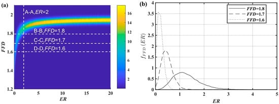
Figure 9. (a) Joint probability distribution of $\mathrm{FFD}$; (b) Marginal probability density of $f_{\mathrm{FFD}}\left(\mathrm{ER}\right)$.

Figure 9a shows the topography of $g\left(\mathrm{ER},\mathrm{FFD}\right)$. Section A is normally distributed. The sections B~C are the marginal probability densities ($y=f_{\mathrm{FFD}}\left(\mathrm{ER}\right)$) after normalization, as shown in Figure 9b. The sensitivity range of the $\mathrm{FFD}$ was investigated using the upper quantiles.

$$\mathrm{P}\left\{\mathrm{ER}>{\mathrm{ER}}_{\alpha }\right\}={\int }_{{\mathrm{ER}}_{\alpha }}^{+\infty }{f}_{\mathrm{FFD}}\left(\mathrm{ER}\right)\mathrm{d}\mathrm{ER}=\alpha$$

(18)

$\alpha$ is a constant value and $0<\alpha <1$. $E{R}_{\alpha }$ is the upper $\alpha$ quantile of $\mathrm{ER}$. If $\alpha =0.05$, there is a 95% probability that the sampled $\mathrm{ER}$ value is less than the ${\mathrm{ER}}_{\alpha }$. The upper $\alpha$ quantile with different $\mathrm{FDs}$ is plotted in Figure 10a.

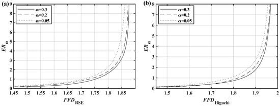
Figure 10. The variation in the upper quantile ${\mathrm{ER}}_{\alpha }$ with (a) ${\mathrm{FFD}}_{\mathrm{R}\mathrm{S}\mathrm{E}}$ and (b) ${\mathrm{FFD}}_{\mathrm{H}\mathrm{i}\mathrm{g}\mathrm{u}\mathrm{c}\mathrm{h}\mathrm{i}}$ when $\alpha =0.3, 0.2, 0.05$. When ${\mathrm{FFD}}_{\mathrm{R}\mathrm{S}\mathrm{E}}>1.8$ or ${\mathrm{FFD}}_{\mathrm{H}\mathrm{i}\mathrm{g}\mathrm{u}\mathrm{c}\mathrm{h}\mathrm{i}}>1.9$, as $\mathrm{FFD}$ increases, ${\mathrm{ER}}_{\alpha }$ increases rapidly and the accuracy of $\mathrm{FFD}$ assessment of $\mathrm{ER}$ decreases rapidly. At this point, small $\mathrm{FFD}$ changes are equivalent to large $\mathrm{ER}$ changes.

The ${\mathrm{FFD}}_{\mathrm{H}\mathrm{i}\mathrm{g}\mathrm{u}\mathrm{c}\mathrm{h}\mathrm{i}}$ was analyzed following the same process yielded in Figure 10b. The ${\mathrm{ER}}_{\alpha }$ rapidly increased when $\mathrm{FFD}>1.8$, indicating a substantial decrease in the sensitivity of the $\mathrm{FFD}$. The exact size of the $\mathrm{ER}$ could not be reliably estimated when ${\mathrm{FFD}}_{\mathrm{R}\mathrm{S}\mathrm{E}}>1.9$. The upper limit of the sensitivity range with the curve of $\alpha =0.3$ was determined, resulting in ${\mathrm{FFD}}_{\mathrm{R}\mathrm{S}\mathrm{E},\mathrm{u}\mathrm{p}}=1.87$, ${\mathrm{FFD}}_{\mathrm{H}\mathrm{i}\mathrm{g}\mathrm{u}\mathrm{c}\mathrm{h}\mathrm{i},\mathrm{u}\mathrm{p}}=1.96$, and ${\mathrm{ER}}_{\mathrm{u}\mathrm{p}}\approx 5$. When $\mathrm{FFD}<1.5$, the $y_{\alpha }$ was almost constant and the $\mathrm{FFD}$ could not estimate how small the $\mathrm{ER}$ was; thus, ${\mathrm{FFD}}_{\mathrm{R}\mathrm{S}\mathrm{E},\mathrm{d}\mathrm{o}\mathrm{w}\mathrm{n}}={\mathrm{FFD}}_{\mathrm{H}\mathrm{i}\mathrm{g}\mathrm{u}\mathrm{c}\mathrm{h}\mathrm{i},\mathrm{d}\mathrm{o}\mathrm{w}\mathrm{n}}=1.5$ and ${\mathrm{ER}}_{\mathrm{d}\mathrm{o}\mathrm{w}\mathrm{n}}\approx 0$. Therefore, the sensitivity range of the $\mathrm{ER}$ was $0~5$. To summarize, beyond this range but less than 2, the FFD cannot reliably estimate the ER size and completely loses its distinguishing ability, but can represent the relative size. The sensitivity range is also a property of the FD, which is why the FD cannot analyze signals with a large ER.

2.5. High-Frequency Suppression Filter

The previous section constructed the FC-Curve, which describes the relationship between the FFD and ER. An HSF was proposed so the FFD could analyze signals with a large ER. The HSF enhances the FFD’s resolution by suppressing the ER within the sensitivity range and functions according to ${Len}_{\mathrm{e}}$. The HSF does not consider the phase deviation problem, and its normalized design is as follows.

$${\Omega }_e={\displaystyle \frac{f_e}{F_s/2}}$$

(19)

where $f_e$ is the filter suppression frequency limit, and ${\Omega }_e$ is the normalized suppression limit of the filter. Combining Equation (11) and Equation (19) yields Equation (20).

$${\Omega }_e=2/{Len}_e$$

(20)

The design of the normalized filter is only related to ${Len}_e$. The suppression ratio is key to the design of the HSF, which mainly refers to the filter’s ability to suppress high frequencies. The definitions are as follows.

$$S=\sum {\Omega }_{\mathrm{High},\mathrm{S}}^2/\sum {\Omega }_{\mathrm{High}}^2$$

(21)

where ${\Omega }_{\mathrm{High}}=\left\{\Omega \left|\Omega >{\Omega }_e, \Omega \in {\Omega }_{\mathrm{original}}\right.\right\}$, and ${\Omega }_{\mathrm{High},\mathrm{S}}=\left\{\Omega \left|\Omega >{\Omega }_e, \Omega \in {\Omega }_{\mathrm{Suppress}}\right.\right\}$. ${\Omega }_{\mathrm{original}}$ is the normalized frequency component of the original signal. ${\Omega }_{\mathrm{Suppress}}$ is the normalized frequency component of the signal after implementing the HSF. Equation (21) means that when the suppression ratio is $S$, the amplitude correction ratio for each frequency component is $\sqrt{S}$.

The filter is designed according to the linear shift-invariant system [38]. The low-frequency amplitude is constant and the high-frequency is suppressed by a factor of $\sqrt{S}$. A linear shift-invariant system can be described by a constant coefficient linear difference equation as follows.

$$y\left(n\right)=-\sum _{k=1}^{N}a\left(k\right)y\left(n-k\right)+\sum _{r=0}^{M}b\left(r\right)x\left(n-r\right)$$

(22)

where $y\left(n\right)$ is the output of the system, $x\left(n\right)$ is the input of the system, and $a, b$ are constants. The output of the system $y\left(n\right)$ is the sum of the historical data $y$ and the new data $x$ of the system.

When filtering a signal, the unit sampling response $h\left(n\right)$ of the system can be convolved with the input $x\left(n\right)$ of the system, as calculated below.

$$y\left(n\right)=\sum _{k=-\infty }^{\infty }x\left(k\right)h\left(n-k\right)=x\left(n\right)*h\left(n\right)$$

(23)

where $\left[*\right]$ denotes a convolution. In the z-transformation, $z=e^{j\omega }$. The filtering in the time domain is $y\left(n\right)=x\left(n\right)*h\left(n\right)$. Correspondingly, the filtering in the frequency domain is $Y\left(e^{j\omega }\right)=X\left(e^{j\omega }\right)H\left(e^{j\omega }\right)$, so $Y\left(z\right)=X\left(z\right)H\left(z\right)$. Combined with Fourier transform results of Equation (22), the following equation can be obtained.

$$H\left(z\right)={\displaystyle \frac{Y\left(z\right)}{X\left(z\right)}}={\displaystyle \frac{{\sum }_{r=0}^{M}b\left(r\right)z^{-r}}{1+{\sum }_{k=0}^{N}a\left(k\right)z^{-k}}}$$

(24)

Factorization gives the following equation.

$$H\left(z\right)=g{z}^{N-M}{\displaystyle \frac{{\prod }_{r=1}^M\left(z-z_r\right)}{{\prod }_{k=1}^N\left(z-p_k\right)}}$$

(25)

where $g$ is the gain factor of the system, $g=b\left(0\right)$. The $p_k$ that makes the denominator zero is the pole point. The $z_r$ that makes the numerator zero is the zero point. The zero and pole of the system is the key point in designing the filter. The unit circle in the complex plane is the key dividing line, as shown by the dashed circle in Figure 11a. When $p_k$ lies on the unit circle, then the frequency at that location passes through without attenuation. In order for the system to converge, $p_k$ can only lie within the unit circle. When $z_r$ lies on the unit circle, the frequency at that position is completely suppressed, which is the design reference for comb filters. And when $z_r$ lies outside the unit circle, the frequency at that position is somewhat attenuated.

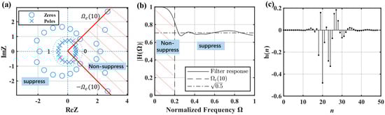
Figure 11. Filter5 features: (a) Zero−pole distribution, the intrinsic characteristics of the filter system; (b) Amplitude frequency response, filtering effect on the frequency domain; (c) Unit sampling response, time domain properties.

Take the design of Filter6 shown in Table 2 as an example. The designed HSF suppresses the frequency components after ${\Omega }_e$ ($f_e$ before normalization), as shown in the ‘suppress’ section of Figure 11a,b. The frequency before ${\Omega }_e$ is guaranteed to pass as losslessly as possible, as shown in the ‘non-suppress’ section of Figure 11a,b. By arranging the zeros and poles as in Figure 11a, the normalized frequency response $H\left(\Omega \right)$ of Figure 11b is thus obtained. Located in the 0~0.2 before ${\Omega }_e$, the response is as close to 1 as possible, while located in 0.2~1, the frequency domain is suppressed by a factor of $\sqrt{0.5}$. Figure 11c is the unit sampling response $h\left(n\right)$, which can be used to obtain filtered result $y\left(n\right)$ according to Equation (23).

Table 2. Normalized original HSF parameters.

$\mathit{L}\mathit{e}{\mathit{n}}_{\mathit{e}} \mathbf{o}\mathbf{r} {\mathit{k}}_{\mathit{e}}$	${\mathit{\Omega }}_{\mathit{e}}$	Filter	Unit Sampling Response (Left to Right, Top to Bottom)
4	0.5	Filter1	9.102 × 10−6	−3.323 × 10−5	6.711 × 10−5	−2.614 × 10−4	−1.265 × 10−4	−2.023 × 10−4	−2.384 × 10−3
			−1.434 × 10−3	1.915 × 10−4	−1.540 × 10−2	−2.172 × 10−2	1.017 × 10−2	2.272 × 10−2	−1.241 × 10−1
			−3.650 × 10−1	−4.497 × 10−1	−2.402 × 10−1	1.502 × 10−1	5.180 × 10−2	1.787 × 10−1	−3.965 × 10−1
			2.108 × 10−1	1.034 × 10−1	−1.644 × 10−1	1.640 × 10−2	7.506 × 10−2	−3.241 × 10−2	−2.597 × 10−2
			2.125 × 10−2	8.103 × 10−3	−1.223 × 10−2	−1.871 × 10−3	6.218 × 10−3	3.128 × 10−4	−3.210 × 10−3
			−1.773 × 10−4	2.009 × 10−3	2.824 × 10−4	−2.106 × 10−3	8.833 × 10−4	9.268 × 10−4	/
5	0.4	Filter2	4.970 × 10−6	−3.181 × 10−5	9.193 × 10−5	−1.837 × 10−4	−3.666 × 10−5	4.037 × 10−4	−8.269 × 10−4
			−2.041 × 10−3	3.321 × 10−3	−9.293 × 10−4	−9.664 × 10−3	−1.929 × 10−2	1.498 × 10−2	4.094 × 10−2
			−3.881 × 10−2	−4.356 × 10−2	−5.116 × 10−1	−8.968 × 10−2	−5.118 × 10−1	−7.428 × 10−2	3.216 × 10−1
			6.368 × 10−2	−1.656 × 10−1	−5.221 × 10−2	7.380 × 10−2	4.068 × 10−2	−2.882 × 10−2	−2.713 × 10−2
			7.391 × 10−3	1.580 × 10−2	1.246 × 10−3	−6.842 × 10−3	−6.450 × 10−3	4.940 × 10−3	5.010 × 10−3
			−2.724 × 10−3	−3.178 × 10−3	1.103 × 10−3	1.834 × 10−3	−2.329 × 10−4	−1.003 × 10−3	/
6	0.333	Filter3	6.072 × 10−6	−3.057 × 10−5	8.098 × 10−5	−5.820 × 10−5	−3.842 × 10−4	4.059 × 10−4	8.329 × 10−4
			−3.726 × 10−3	−6.739 × 10−3	3.521 × 10−4	1.869 × 10−2	9.110 × 10−3	−4.600 × 10−2	−1.675 × 10−1
			−2.838 × 10−1	−3.025 × 10−1	−3.521 × 10−1	9.422 × 10−2	−2.449 × 10−1	3.883 × 10−1	1.223 × 10−1
			−2.550 × 10−1	−1.071 × 10−1	1.103 × 10−1	8.542 × 10−2	−2.520 × 10−2	−5.346 × 10−2	−8.410 × 10−3
			2.268 × 10−2	1.516 × 10−2	−4.159 × 10−3	−1.026 × 10−2	−3.417 × 10−3	3.222 × 10−3	4.042 × 10−3
			2.442 × 10−3	−3.830 × 10−3	−3.122 × 10−3	1.879 × 10−3	2.408 × 10−3	−3.287 × 10−4	/
7	0.286	Filter4	−3.505 × 10−3	8.280 × 10−3	2.039 × 10−2	1.552 × 10−2	−3.050 × 10−2	−1.063 × 10−1	−2.034 × 10−1
			−2.580 × 10−1	−2.721 × 10−1	−2.100 × 10−1	−6.624 × 10−2	−9.047 × 10−2	2.982 × 10−1	−2.076 × 10−1
			2.692 × 10−1	4.264 × 10−2	−3.034 × 10−1	−9.466 × 10−2	1.680 × 10−1	1.394 × 10−1	−2.134 × 10−2
8	0.25		−9.730 × 10−2	−5.023 × 10−2	2.053 × 10−2	4.506 × 10−2	2.196 × 10−2	−8.569 × 10−3	−2.051 × 10−2
			−1.250 × 10−2	1.464 × 10−3	9.194 × 10−3	8.611 × 10−3	1.626 × 10−3	−4.045 × 10−3	−4.483 × 10−3
			−6.285 × 10−3	1.048 × 10−3	8.891 × 10−3	4.319 × 10−3	−4.523 × 10−3	−5.896 × 10−3	/
9	0.222	Filter5	−1.197 × 10−3	−2.031 × 10−3	−2.067 × 10−3	4.012 × 10−3	7.027 × 10−3	1.727 × 10−2	6.506 × 10−3
			−1.439 × 10−2	1.027 × 10−2	−2.284 × 10−1	1.595 × 10−1	−4.807 × 10−1	−1.118 × 10−1	2.559 × 10−2
10	0.2		−2.807 × 10−1	−3.292 × 10−1	−7.498 × 10−2	1.498 × 10−1	1.846 × 10−1	8.476 × 10−2	−2.276 × 10−2
			−6.935 × 10−2	−5.613 × 10−2	−1.914 × 10−2	1.078 × 10−2	2.169 × 10−2	1.731 × 10−2	7.067 × 10−3
11	0.182		−2.079 × 10−3	−6.233 × 10−3	−5.806 × 10−3	−4.274 × 10−3	−1.509 × 10−3	2.181 × 10−3	4.025 × 10−3
			2.783 × 10−3	1.261 × 10−4	−1.685 × 10−3	−1.805 × 10−3	−8.370 × 10−4	1.996 × 10−4	/
12	0.167	Filter6	5.429 × 10−8	−2.324 × 10−7	−3.348 × 10−7	2.879 × 10−6	5.870 × 10−6	−1.359 × 10−5	−5.555 × 10−5
			−4.885 × 10−5	2.117 × 10−4	8.570 × 10−4	2.064 × 10−3	3.163 × 10−3	4.373 × 10−3	2.553 × 10−3
13	0.154		1.184 × 10−3	−9.877 × 10−3	−1.916 × 10−2	−2.309 × 10−2	−1.280 × 10−1	1.124 × 10−1	−4.558 × 10−1
			1.367 × 10−1	−5.846 × 10−2	−4.089 × 10−1	−3.342 × 10−1	−8.752 × 10−2	7.801 × 10−2	1.170 × 10−1
14	0.143		8.097 × 10−2	3.031 × 10−2	−4.424 × 10−3	−1.764 × 10−2	−1.656 × 10−2	−9.886 × 10−3	−3.426 × 10−3
			5.845 × 10−4	2.144 × 10−3	2.142 × 10−3	1.483 × 10−3	7.292 × 10−4	1.870 × 10−4	/

If the convolution result exists, the convolution satisfies the distributive law. This means that it is possible to self-convolve the original filters in advance to obtain filters with different suppression ratios. The filter elongates due to the convolution, which discards smaller values at both ends.

$$h\left(n\right)=\mathrm{Filter}N\left(n\right)=\underset{n}{\underbrace{\mathrm{Filter}N\otimes \cdots \otimes \mathrm{Filter}N}}$$

(26)

where $N$ is the original filter number. The $S$ of $\mathrm{Filter}N\left(n\right)$ is $0.5^n$. Table 2 shows the normalized filter parameters. The approximate ${Len}_e$ shares a common original filter. The order of the filter was selected based on historical data. The calculated $\mathrm{Filter}N\left(n\right)$ is $h\left(n\right)$ in Equation (23). Determine the selection of the original filter according to Equations (13) and (14). It can also be selected according to self-defined ${\Omega }_e$.

When monitoring the milling process, the sensors should be mounted in a moderately stable location, such as the spindle housing [39]. Figure 12 shows the filtering effect of s2 in Table 5. The characterization of s2 can be observed in Figure 19. When $R=1~12$ was taken to calculate the original ${\mathrm{FFD}}_{\mathrm{H}\mathrm{i}\mathrm{g}\mathrm{u}\mathrm{c}\mathrm{h}\mathrm{i}}$, the sensitivity was reduced as it tended toward 2. This problem was similar to that with the traditional FD. The ${\mathrm{FFD}}_{\mathrm{H}\mathrm{i}\mathrm{g}\mathrm{u}\mathrm{c}\mathrm{h}\mathrm{i}}$ distinguished between stability and chatter after filtering with Filter1(4). The $\mathrm{ER}$ remained large after using the HSF when the $\mathrm{ER}$ was large from 7 s to 13 s, so the ${\mathrm{FFD}}_{\mathrm{H}\mathrm{i}\mathrm{g}\mathrm{u}\mathrm{c}\mathrm{h}\mathrm{i}}$ only showed a smaller decrease. However, if the $\mathrm{ER}$ was not so large from 0 s to 7 s, it tended toward 0 after using the HSF, so the ${\mathrm{FFD}}_{\mathrm{H}\mathrm{i}\mathrm{g}\mathrm{u}\mathrm{c}\mathrm{h}\mathrm{i}}$ significantly decreased. The calculations based on actual signals show that the HSF adjusted the signal $\mathrm{ER}$, allowing the $\mathrm{FFD}$ to effectively analyze the signal with a larger ER. An abnormality appeared as expected when calculating the ${\mathrm{FFD}}_{\mathrm{H}\mathrm{i}\mathrm{g}\mathrm{u}\mathrm{c}\mathrm{h}\mathrm{i}}$ with the parameter ($R=7~19$) in Figure 8. This shows that the region for calculating the ${\mathrm{FFD}}_{\mathrm{H}\mathrm{i}\mathrm{g}\mathrm{u}\mathrm{c}\mathrm{h}\mathrm{i}}$ cannot be chosen arbitrarily.

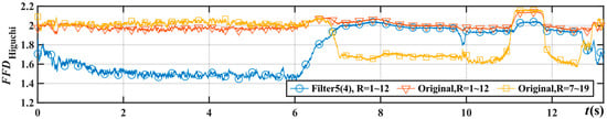
Figure 12. Comparison of the HSF filtering effect on the results of s1 experimental data in Table 5.

3. Application

A milling chatter acceleration signal is a typical kind of signal with a large ER. The traditional FD tends to lose its resolution when analyzing such signals. Sample delay and calculation delay are defined to compare different methods in chatter identification. Figure 13 describes the chatter monitoring process. After chatter occurs, the chatter alarm does not occur until after the detection delay, which is the sum of the sample delay and calculation delay. The smaller the detection delay, the faster the chatter suppression is achieved and the less surface damage there is. When chatter is suppressed, the alarm is canceled after the feedback delay, which is the sum of the sample delay and calculation delay. If the feedback delay is too long, the chatter suppression process may overshoot and lead to system instability. Therefore, only methods with a small sample delay and calculation delay are suitable for real-time monitoring.

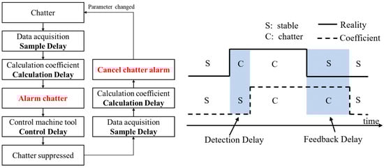
Figure 13. Flowchart of real-time chatter monitoring process and the definition of delays.

3.1. Fast Energy Ratio Indicator

In this study, the FER is proposed based on the FC-Curve and the HSF. The FER normalizes the chatter index to 0~1 via the FFD sensitivity range. The sensitivity range is discussed in Section 2.4.

$${\mathrm{FER}}_n=h\left({\mathrm{FFD}}_n\right)=\left\{\begin{array}{cc}1& ,{\mathrm{FFD}}_n>{\mathrm{FFD}}_{\mathrm{up}}\\ ({\mathrm{FFD}}_n-{\mathrm{FFD}}_{\mathrm{down}})/\left({\mathrm{FFD}}_{\mathrm{down}}-{\mathrm{FFD}}_{\mathrm{up}}\right)& ,{\mathrm{FFD}}_{\mathrm{down}}<{\mathrm{FD}}_n<{\mathrm{FFD}}_{\mathrm{up}}\\ 0& ,{\mathrm{FFD}}_n<{\mathrm{FFD}}_{\mathrm{down}}\end{array}\right.$$

(27)

where ${\mathrm{FFD}}_{\mathrm{up}}$–${\mathrm{FFD}}_{\mathrm{down}}$ is the sensitivity range. Figure 14 shows the flowchart of online flutter monitoring, and 192 data were chosen. FER and FFD methods are able to deal with the online monitoring of signals because of their fast speed and lower calculation workload. Therefore, it can be expected to apply in various areas including chatter signals in machining, bioelectrical signals, and wear and aging signals of engineering devices.

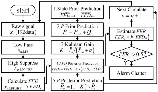
Figure 14. Process of calculating FER. The first column is the acquisition of data and preprocessing to obtain ${\mathrm{FFD}}_n$; the second column is the five processes of Kalman filtering; and the third column is the calculation of ${\mathrm{FER}}_n$ to identify chatter.

Kalman filtering was needed to reduce the noise. The acquired data were passed through a low-pass filter (LPF) and HSF to calculate the $\mathrm{FFD}$. After Kalman filtering, a relatively stable ${\overline{FFD}}_n$ was obtained. Finally, after Equation (27), ${\mathrm{FER}}_n$. $Fs=\mathrm{25,600} \mathrm{H}\mathrm{z}$, the sample delay was 7.5 ms, and the data overlap was 75%. It was approximated that the ER was unchanged in the Kalman filtering process due to the 75% overlap. In Step 1, ${\widetilde{FFD}}_n={\overline{FFD}}_{n-1}$, and the prediction error was $Q=0.0001$, where ${\widetilde{FFD}}_n$ is an a priori estimate, and ${\overline{FFD}}_{n-1}$ is the a posteriori estimate. The prediction variance $\mathrm{P}$ was also updated. The computational error for the new data was obtained from Figure 4b and Figure 6b, and $\sigma =0.02$. Step 1~Step 5 was repeated continuously to achieve real-time data filtering.

3.2. Simulation Verification

The computer CPU was Intel(R) Core (TM) i7-13700KF, and the software was MATLAB 2022a. The sampling frequency was 25,600 Hz. A speed of 10,000 r/min and a 2-tooth cutter were used in the experiment. The chatter interval was set to 3500 Hz~4500 Hz. The ER was approximately 1 when stable and approximately 100 when chatter occurred. The signal duration was 6 s.

$$\begin{array}{l}Sig=Si{g}_s+Si{g}_c+Si{g}_n\\ Si{g}_s={\displaystyle \sum _{i=1}^{70}}{1.2}^{-1.4i}\cos \left(2\pi f_{b}it+\phi \right)+{\displaystyle \sum _{i=1}^{10}}{1.5}^{-1.4i}\cos \left(2\times 2\pi f_{b}it+\phi \right)\\ Si{g}_c=\left\{\begin{array}{cc}20\mathit{cos}\left(7000\pi t+\mathit{cos}\left(1000t\right)\right)\times \mathit{cos}\left(150\pi t+\mathit{cos}\left(2000t\right)\right),& 2<t<4\\ \mathit{cos}\left(7000\pi t+\mathit{cos}\left(1000t\right)\right)\times \mathit{cos}\left(150\pi t+\mathit{cos}\left(2000t\right)\right),& \mathrm{else}\end{array}\right.\end{array}$$

(28)

where $Si{g}_s$ is the stable component, which consists of the fundamental frequency and the tooth passing frequency. $Si{g}_c$ is the chatter component. To better simulate the actual signal, 2–4 s is a severe chatter, and a smaller chatter component still exists when idle. $Si{g}_n$ is the noise component, and a noise of 10 dB is introduced during the calculation. $\phi$ is the random phase. The simulated signal is shown in Figure 15.

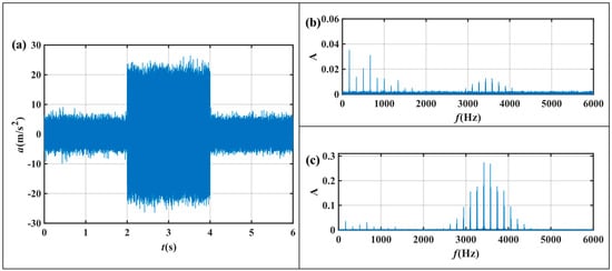
Figure 15. Artificial signal: (a) time domain signal characteristics; frequency domain characteristics of (b) stable and (c) chatter.

The window had a length of 192 data. The contrasting algorithm was the energy ratio difference ($\mathrm{ERD}$) [40] based on the VMD and the energy entropy ($\mathrm{P}$) based on the wavelet packet decomposition (WPD) [33]. The WPD parameters to calculate $\mathrm{P}$ were db3 wavelet bases and three-order decompositions. The chatter interval of the $\mathrm{ERD}$ was set to 3500 Hz~4500 Hz. The effect of sample delay was added when plotted in Figure 16.

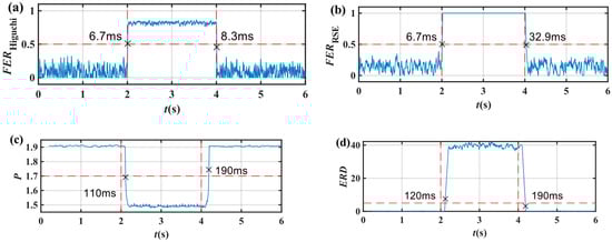
Figure 16. Chatter detection performance of different methods: (a) ${\mathrm{FER}}_{\mathrm{H}\mathrm{i}\mathrm{g}\mathrm{u}\mathrm{c}\mathrm{h}\mathrm{i}}$; (b) ${\mathrm{FER}}_{\mathrm{R}\mathrm{S}\mathrm{E}}$; (c) $\mathrm{P}$; (d) $\mathrm{ERD}$; The horizontal dashed line is the threshold; The vertical dashed line is the transition time, 2 s for the first and 4 s for the second.

Table 3 summarizes the delay results for the different methods. The detection delays of the $\mathrm{FER},$ $\mathrm{ERD},$ and $\mathrm{P}$ were 6.7 ms, 120 ms, and 110 ms, respectively. The feedback delays of the ${\mathrm{FER}}_{\mathrm{H}\mathrm{i}\mathrm{g}\mathrm{u}\mathrm{c}\mathrm{h}\mathrm{i}}$ and ${\mathrm{FER}}_{\mathrm{R}\mathrm{S}\mathrm{E}}$ were 8.3 ms and 32.9 ms, respectively, while those of the $\mathrm{ERD}$ and $\mathrm{P}$ were 190 ms. The delay of the $\mathrm{FER}$ was smaller, so the $\mathrm{FER}$ can better reflect the system’s current state in real time. Furthermore, the ${\mathrm{FER}}_{\mathrm{H}\mathrm{i}\mathrm{g}\mathrm{u}\mathrm{c}\mathrm{h}\mathrm{i}}$ calculation only required 21 μs, while the $\mathrm{ERD}$ based on VMD needed 79 ms. Therefore, the $\mathrm{FER}$ has higher computational efficiency and is more suitable for online monitoring.

Table 3. Chatter detection performance of different methods (Fs = 25,600).

Method	Window Length (ms, Data)	Overlap (ms, Data)	Total Time (s)	Mean Time (ms)	Detection Delay (ms)	Feedback Delay (ms)
${\mathrm{FER}}_{\mathrm{H}\mathrm{i}\mathrm{g}\mathrm{u}\mathrm{c}\mathrm{h}\mathrm{i}}$	7.5, 192	5.625, 144	0.109	0.0214	6.7	8.3
${\mathrm{FER}}_{\mathrm{R}\mathrm{S}\mathrm{E}}$	7.5, 192	5.625, 144	1.405	0.275	6.7	32.9
$\mathrm{P}$	100, 2560	90, 2304	3.014	5.109	110	190
$\mathrm{ERD}$	100, 2560	90, 2304	46.62	79.03	120	190

3.3. Milling Experiment

The milling experiments were performed with a 3-axis machine tool. The workpiece material was Al7075, and the size was 150 × 85 × 8 mm. A vise was used to clamp the workpiece, which extended to 45 mm. The size of the vise was 150 mm wide and 40 mm deep. The cutter parameters are shown in Table 4. Acceleration sensors were generally arranged close to the machining area, such as on the workpiece or spindle housing [39,40].

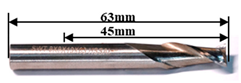
Table 4. Parameters of the cutting tool.

2-Edge Cutter	Diameter	Length	Overhang	Edge Length	Material
	8 mm	63 mm	45 mm	19 mm	High-speed steel

The milling vibration on workpieces is very high, so the vibration on a spindle is suitable for chatter monitoring [30,41]. The milling experiment layout is shown in Figure 17. The data used for the analysis were obtained from the PCB356A24 sensor, SN266885, products of PCB Piezotronics from America. The signal acquisition device was the LMS SCADAS Mobile, products of Siemens from Germany. The CPU of the data-processing computer was Intel(R) Core(TM) i7-13700KF, and the software was MATLAB 2022a. A variable depth of cut scheme was used. The machining parameters were set as listed in Table 5.

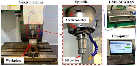
Figure 17. Setup of the milling experiments on 3-axis machines.

Table 5. Experimental parameters.

Number	Speed (r/min)	Feed Speed (mm/min)	Axial Depth (mm)	Radial Depth (mm)
s1	10,000	1000	2~10	4
s2	7000	700	2~10	4
s3	4000	700	2~10	4
s4	10,000	720	2~10	4
s5	10,000	600	2~10	4

Next, two sets of signals, s1 and s2, were analyzed. In this study, the surface damage and the short-time Fourier transform (STFT) results were used to determine the occurrence of severe vibration. The side surface damage was selected as a reference for chatter. Pictures of the sides were taken using an electron microscope and stitched together into one image.

3.4. Analysis of Experiment s1

The results of s1 are shown in Figure 18, where the red vertical dashed lines represent the correspondence between (a) surface features, (b) state labels, (c) STFT, (d) time domain signals, and (e~i) the calculated results. The ‘×’ symbol represents the time to recognize chatter and (b) is the milling state determined based on (a) and (c). The first and last 4 mm in (a) stand for cutting in and out, respectively. Since $\mathrm{ERD}$ needed to set the chatter interval, it failed to recognize the chatter of 4000 Hz~5000 Hz after 8.7 s. The frequency distribution of some chatter states was more uniform. Therefore, $\mathrm{P}$ also failed to identify the chatter in 8.7 s. $\mathrm{FER}$ and $\mathrm{FD}$ produced some mistakes in the cut-in process.

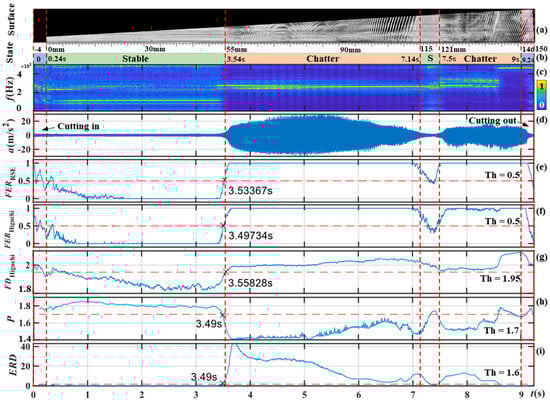
Figure 18. Comparison of the analysis results of the s1 signal: (a) Surface morphology of the workpiece; (b) milling state determined according to (a,c), S is stable and C is chatter; (c) Normalized short−time Fourier transform; (d) Time domain; (e) ${\mathrm{FER}}_{\mathrm{R}\mathrm{S}\mathrm{E}}$; (f) ${\mathrm{FER}}_{\mathrm{H}\mathrm{i}\mathrm{g}\mathrm{u}\mathrm{c}\mathrm{h}\mathrm{i}}$; (g) ${\mathrm{FD}}_{\mathrm{H}\mathrm{i}\mathrm{g}\mathrm{u}\mathrm{c}\mathrm{h}\mathrm{i}}$; (h) $\mathrm{P}$; (i) $\mathrm{ERD}$; The horizontal dashed line is the threshold; The vertical dashed line is the transition time.

The latency of the chatter alarm for 55 mm (3.54 s) is shown in Table 6. Considering the sample delay and calculation delay, ${\mathrm{FER}}_{\mathrm{H}\mathrm{i}\mathrm{g}\mathrm{u}\mathrm{c}\mathrm{h}\mathrm{i}}$ and $\mathrm{P}$ could still detect chatter at −40 ms, so they produced the best recognition results. The calculation delay of $\mathrm{P}$ was 5.9 ms, which was larger than that of ${\mathrm{FER}}_{\mathrm{H}\mathrm{i}\mathrm{g}\mathrm{u}\mathrm{c}\mathrm{h}\mathrm{i}} \mathrm{o}\mathrm{f} 20.6 \mathsf{\mu }\mathrm{s}$. ${\mathrm{FD}}_{\mathrm{H}\mathrm{i}\mathrm{g}\mathrm{u}\mathrm{c}\mathrm{h}\mathrm{i}}$ selected 1.95 as the $\mathrm{T}\mathrm{h}$ (Threshold) and identified chatter at 18.28 ms. The $\mathrm{FD}$ was less able to discriminate without the HSF. The $\mathrm{ERD}$ was a successful offline calculation method, but the calculation delay was 91.6 ms, which is too large for online chatter monitoring. The $\mathrm{ERD}$ identified chatter at 41.6 ms, the worst result. The $\mathrm{FER}$ is a more suitable method for online monitoring.

Table 6. Result of s1, Fs = 25,600 Hz.

Signal: s1	Sample Delay (ms, Data)	Detection Delay (ms) (Without Calculation)	Calculation Delay (ms)	Detection Delay (ms) (With Calculation)
${\mathrm{FER}}_{\mathrm{R}\mathrm{S}\mathrm{E}}$	7.5, 192	−6.33	0.279	−6.609
${\mathrm{FER}}_{\mathrm{H}\mathrm{i}\mathrm{g}\mathrm{u}\mathrm{c}\mathrm{h}\mathrm{i}}$	7.5, 192	−42.66	0.0206	−42.6806
${\mathrm{FD}}_{\mathrm{H}\mathrm{i}\mathrm{g}\mathrm{u}\mathrm{c}\mathrm{h}\mathrm{i}}$	7.5, 192	18.28	0.0132	18.2932
$\mathrm{P}$	100, 2560	−50	5.905	−44.095
$\mathrm{ERD}$	100, 2560	−50	91.6	41.6

The surface from 7.14 s to 7.5 s was a transitional state with a shallow chattering texture, and the surface quality was better, which was a kind of transition milling state. The $\mathrm{FER}$ decreased in the transition state, characterized by the stabilization of the milling process. This suggests that the $\mathrm{FER}$ reasonably reflects the steady state of the cutting process.

3.5. Analysis of Experiment s2

The results of s2 are shown in Figure 19. The latency of the chatter alarm for 72 mm (6.5143 s) is shown in Table 7. The ${\mathrm{FER}}_{\mathrm{R}\mathrm{S}\mathrm{E}}$ alarm chatter occurred at −138.553 ms, the best result. ${\mathrm{FER}}_{\mathrm{H}\mathrm{i}\mathrm{g}\mathrm{u}\mathrm{c}\mathrm{h}\mathrm{i}}$ and $\mathrm{P}$ produced similar results, i.e., alarm chatter at approximately 110 ms. However, the calculations of ${\mathrm{FER}}_{\mathrm{H}\mathrm{i}\mathrm{g}\mathrm{u}\mathrm{c}\mathrm{h}\mathrm{i}}$ also took 21.4 μs.

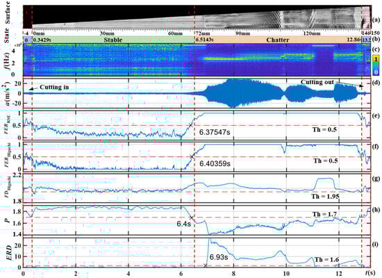
Figure 19. Comparison of the analysis results of the s2 signal: (a) Surface morphology of the workpiece; (b) milling state determined according to (a,c), S is stable and C is chatter; (c) Normalized short−time Fourier transform; (d) Time domain; (e) ${\mathrm{FER}}_{\mathrm{R}\mathrm{S}\mathrm{E}}$; (f) ${\mathrm{FER}}_{\mathrm{H}\mathrm{i}\mathrm{g}\mathrm{u}\mathrm{c}\mathrm{h}\mathrm{i}}$; (g) ${\mathrm{FD}}_{\mathrm{H}\mathrm{i}\mathrm{g}\mathrm{u}\mathrm{c}\mathrm{h}\mathrm{i}}$; (h) $\mathrm{P}$; (i) $\mathrm{ERD}$; The horizontal dashed line is the threshold; The vertical dashed line is the transition time.

Table 7. Result of s2, Fs = 25,600 Hz.

Signal: s2	Sample Delay (ms, Data)	Detection Delay (ms) (Without Calculation)	Calculation Delay (ms)	Detection Delay (ms) (With Calculation)
${\mathrm{FER}}_{\mathrm{R}\mathrm{S}\mathrm{E}}$	7.5, 192	−138.83	0.277	−138.553
${\mathrm{FER}}_{\mathrm{H}\mathrm{i}\mathrm{g}\mathrm{u}\mathrm{c}\mathrm{h}\mathrm{i}}$	7.5, 192	−110.71	0.0214	−110.689
${\mathrm{FD}}_{\mathrm{H}\mathrm{i}\mathrm{g}\mathrm{u}\mathrm{c}\mathrm{h}\mathrm{i}}$	7.5, 192	/	0.0128	/
$\mathrm{P}$	100, 2560	−114.3	5.223	−109.077
$\mathrm{ERD}$	100, 2560	415.7	91.6	507.3

The $HFD$ could not identify chatter without the HSF because the $\mathrm{ER}$ was too large. The $\mathrm{ERD}$ failed to recognize the chatter of 4000 Hz~5000 Hz at 6.5 s~7 s and 11.5 s~12 s. While severe chatter still featured at 11.5 s~12 s, the characteristic values of $\mathrm{P}$ and $\mathrm{ERD}$ approached the threshold, and P was almost misclassified. Conversely, the $\mathrm{FER}$ stabilized away from the threshold with severe chattering, making misidentification unlikely. In addition, evolution towards stabilization occurred at 9.8 s, and the $\mathrm{FER}$ decreased simultaneously. This suggests that the $\mathrm{FER}$ is a reliable method for describing the state of the milling process. The $\mathrm{FER}$ is more suitable for online monitoring scenarios because it describes the milling state and is less computationally time-consuming.

4. Conclusions

The FD can reflect the characteristics of the frequency domain in the time domain, highlighting its good application prospects in engineering applications. Many non-fractal digital signals in engineering lack a mathematical FD, and obtaining the correct FD is meaningless. However, engineering applications have shown that the frequency-domain features of non-fractal signals can still be obtained using the FD. A new system of fractal analysis was proposed in this study to fill this gap in the research. It is worth noting that the calculations of FD and FFD are the same, but the interval for the FFD is the fixed interval proposed in this paper. The conclusions of this paper are an expansion of the traditional FD. Therefore, there are similarities in the nature of FD and FFD. The key conclusions are summarized as follows:

• The relationship between the FFD and ER was determined based on the simulation signal of a variable ER. This relationship was called the FC-Curve, as shown in Equation (16). Different methods and fixed-interval selection strategies had different FC-Curve coefficients. The sensitivity region was determined based on the FC-Curve and variance curve. The sensitivity region was ${\mathrm{FFD}}_{\mathrm{R}\mathrm{S}\mathrm{E}}=1.5~1.85$, ${\mathrm{FFD}}_{\mathrm{H}\mathrm{i}\mathrm{g}\mathrm{u}\mathrm{c}\mathrm{h}\mathrm{i}}=1.5~1.96,$ and $ER=0~5$. The FFD could not reliably estimate the ER size beyond this range or for values less than two; nevertheless, it could still represent the relative size.
• The HSF was proposed in this study as a pioneering approach, significantly enhancing the applicability of the FFD in practical engineering scenarios. The HSF expands the use of the FFD in engineering by suppressing the ER. The FFD tended toward two throughout the milling process without the HSF. The HSF effectively enhanced the resolution of the FFD. The FFD in the stable milling state was reduced from 2 to 1.5, and the flutter state changed only slightly. The HSF and the new fractal analysis system can also be applied to other analytical areas.
• The FER method was proposed based on the need for online chatter monitoring. The simulation results show that the detect delay and feedback delay of ${\mathrm{FER}}_{\mathrm{R}\mathrm{S}\mathrm{E}}$ and ${\mathrm{FER}}_{\mathrm{H}\mathrm{i}\mathrm{g}\mathrm{u}\mathrm{c}\mathrm{h}\mathrm{i}}$ were below 32 ms. The real-time performance was better than that of $\mathrm{P}$ and $\mathrm{ERD}$. The computation time per eigenvalue was 275 μs for ${\mathrm{FER}}_{\mathrm{R}\mathrm{S}\mathrm{E}}$ and 21 μs for ${\mathrm{FER}}_{\mathrm{H}\mathrm{i}\mathrm{g}\mathrm{u}\mathrm{c}\mathrm{h}\mathrm{i}}$, which is more efficient and more suitable for online monitoring.

References

- Raubitzek, S.; Neubauer, T. Combining Measures of Signal Complexity and Machine Learning for Time Series Analyis: A Review. Entropy 2021, 23, 1672. [Google Scholar] [CrossRef]
- Navish, A.A.; Priya, M.; Uthayakumar, R. A Comparative Study on Estimation of Fractal Dimension of EMG Signal Using SWT and FLP. Comput. Methods Biomech. Biomed. Eng. Imaging Vis. 2023, 11, 586–597. [Google Scholar] [CrossRef]
- Chandrasekharan, S.; Jacob, J.E.; Cherian, A.; Iype, T. Exploring Recurrence Quantification Analysis and Fractal Dimension Algorithms for Diagnosis of Encephalopathy. Cogn. Neurodynamics 2024, 18, 133–146. [Google Scholar] [CrossRef]
- Wijayanto, I.; Hartanto, R.; Nugroho, H.A. Multi-Distance Fluctuation Based Dispersion Fractal for Epileptic Seizure Detection in EEG Signal. Biomed. Signal Process. Control 2021, 69, 102938. [Google Scholar] [CrossRef]
- Yuan, Q.; Zhou, W.; Liu, Y.; Wang, J. Epileptic Seizure detection with linear and nonlinear features. Epilepsy Behav. 2012, 24, 415–421. [Google Scholar] [CrossRef]
- Jamshidi, M.; Rimpault, X.; Balazinski, M.; Chatelain, J.-F. Fractal Analysis Implementation for Tool Wear Monitoring Based on Cutting Force Signals during CFRP/Titanium Stack Machining. Int. J. Adv. Manuf. Technol. 2020, 106, 3859–3868. [Google Scholar] [CrossRef]
- Valtierra-Rodriguez, M. Fractal Dimension and Data Mining for Detection of Short-Circuited Turns in Transformers from Vibration Signals. Meas. Sci. Technol. 2020, 31, 025902. [Google Scholar] [CrossRef]
- Shen, Z.; Pan, G.; Yan, Y. A High-Precision Fatigue Detecting Method for Air Traffic Controllers Based on Revised Fractal Dimension Feature. Math. Probl. Eng. 2020, 2020, 4563962. [Google Scholar] [CrossRef]
- Pal, R.; Barney, A. Iterative Envelope Mean Fractal Dimension Filter for the Separation of Crackles from Normal Breath Sounds. Biomed. Signal Process. Control 2021, 66, 102454. [Google Scholar] [CrossRef]
- Chen, Z.; Liu, Y.; Zhou, P. A Comparative Study of Fractal Dimension Calculation Methods for Rough Surface Profiles. Chaos Solitons Fractals 2018, 112, 24–30. [Google Scholar] [CrossRef]
- Zhang, X.; Xu, Y.; Jackson, R.L. An Analysis of Generated Fractal and Measured Rough Surfaces in Regards to Their Multi-Scale Structure and Fractal Dimension. Tribol. Int. 2017, 105, 94–101. [Google Scholar] [CrossRef]
- Li, Z.; Qian, X.; Feng, F.; Qu, T.; Xia, Y.; Zhou, W. A Continuous Variation of Roughness Scaling Characteristics across Fractal and Non-Fractal Profiles. Fractals 2021, 29, 2150109. [Google Scholar] [CrossRef]
- Jamshidi, M.; Chatelain, J.-F.; Rimpault, X.; Balazinski, M. Tool Condition Monitoring Based on the Fractal Analysis of Current and Cutting Force Signals during CFRP Trimming. Int. J. Adv. Manuf. Technol. 2022, 121, 8127–8142. [Google Scholar] [CrossRef]
- Sharma, M.; Pachori, R.B.; Rajendra Acharya, U. A New Approach to Characterize Epileptic Seizures Using Analytic Time-Frequency Flexible Wavelet Transform and Fractal Dimension. Pattern Recognit. Lett. 2017, 94, 172–179. [Google Scholar] [CrossRef]
- Hadiyoso, S.; Wijayanto, I.; Humairani, A. Entropy and Fractal Analysis of EEG Signals for Early Detection of Alzheimer’s Dementia. Trait. Signal 2023, 40, 1673–1679. [Google Scholar] [CrossRef]
- Yang, X.; Xiang, Y.; Jiang, B. On Multi-Fault Detection of Rolling Bearing through Probabilistic Principal Component Analysis Denoising and Higuchi Fractal Dimension Transformation. J. Vib. Control 2022, 28, 1214–1226. [Google Scholar] [CrossRef]
- Namazi, H. Complexity and Information-Based Analysis of the Heart Rate Variability (Hrv) While Sitting, Hand Biking, Walking, and Running. Fractals 2021, 29, 2150201. [Google Scholar] [CrossRef]
- Sobahi, N.; Atila, O.; Deniz, E.; Sengur, A.; Acharya, U.R. Explainable COVID-19 Detection Using Fractal Dimension and Vision Transformer with Grad-CAM on Cough Sounds. Biocybern. Biomed. Eng. 2022, 42, 1066–1080. [Google Scholar] [CrossRef]
- Zhang, Y.; Wu, J.; Hong, X.; He, Y. Short-Circuit Fault Detection in Laminated Long Stators of High-Speed Maglev Track Based on Fractal Dimension. Measurement 2021, 176, 109177. [Google Scholar] [CrossRef]
- Mei, X.; Xu, H.; Feng, P.; Yuan, M.; Xu, C.; Ma, Y.; Feng, F. Online Chatter Monitor System Based on Rapid Detection Method and Wireless Communication. Int. J. Adv. Manuf. Technol. 2022, 122, 1321–1337. [Google Scholar] [CrossRef]
- Ji, Y.; Wang, X.; Liu, Z.; Yan, Z.; Jiao, L.; Wang, D.; Wang, J. EEMD-Based Online Milling Chatter Detection by Fractal Dimension and Power Spectral Entropy. Int. J. Adv. Manuf. Technol. 2017, 92, 1185–1200. [Google Scholar] [CrossRef]
- Ji, Y.; Wang, X.; Liu, Z.; Wang, H.; Jiao, L.; Wang, D.; Leng, S. Early Milling Chatter Identification by Improved Empirical Mode Decomposition and Multi-Indicator Synthetic Evaluation. J. Sound. Vib. 2018, 433, 138–159. [Google Scholar] [CrossRef]
- Zhuo, Y.; Jin, H.; Han, Z. Chatter Identification in Flank Milling of Thin-Walled Blade Based on Fractal Dimension. Procedia Manuf. 2020, 49, 150–154. [Google Scholar] [CrossRef]
- Yan, X.; Tang, G.; Wang, X. A Chaotic Feature Extraction Based on SMMF and CMMFD for Early Fault Diagnosis of Rolling Bearing. IEEE Access 2020, 8, 179497–179515. [Google Scholar] [CrossRef]
- Khodadadi, V.; Nowshiravan Rahatabad, F.; Sheikhani, A.; Jafarnia Dabanloo, N. Nonlinear Analysis of Biceps Surface EMG Signals for Chaotic Approaches. Chaos Solitons Fractals 2023, 166, 112965. [Google Scholar] [CrossRef]
- Liu, T.; Deng, Z.; Luo, C.; Li, Z.; Lv, L.; Zhuo, R. Chatter Detection in Camshaft High-Speed Grinding Process Based on VMD Parametric Optimization. Measurement 2022, 187, 110133. [Google Scholar] [CrossRef]
- Liu, C.; Zhu, L.; Ni, C. Chatter Detection in Milling Process Based on VMD and Energy Entropy. Mech. Syst. Signal Process. 2018, 105, 169–182. [Google Scholar] [CrossRef]
- Cao, H.; Zhou, K.; Chen, X. Chatter Identification in End Milling Process Based on EEMD and Nonlinear Dimensionless Indicators. Int. J. Mach. Tools Manuf. 2015, 92, 52–59. [Google Scholar] [CrossRef]
- Wang, P.; Bai, Q.; Cheng, K.; Zhang, Y.; Zhao, L.; Ding, H. Investigation on an in-process chatter detection strategy for micro-milling titanium alloy thin-walled parts and its implementation perspectives. Mech. Syst. Signal Process. 2023, 183, 109617. [Google Scholar] [CrossRef]
- Yan, S.; Sun, Y. Early Chatter Detection in Thin-Walled Workpiece Milling Process Based on Multi-Synchrosqueezing Transform and Feature Selection. Mech. Syst. Signal Process. 2022, 169, 108622. [Google Scholar] [CrossRef]
- Thomazella, R.; Lopes, W.N.; Aguiar, P.R.; Alexandre, F.A.; Fiocchi, A.A.; Bianchi, E.C. Digital Signal Processing for Self-Vibration Monitoring in Grinding: A New Approach Based on the Time-Frequency Analysis of Vibration Signals. Measurement 2019, 145, 71–83. [Google Scholar] [CrossRef]
- Hao, Y.; Zhu, L.; Yan, B.; Qin, S.; Cui, D.; Lu, H. Milling Chatter Detection with WPD and Power Entropy for Ti-6Al-4V Thin-Walled Parts Based on Multi-Source Signals Fusion. Mech. Syst. Signal Process. 2022, 177, 109225. [Google Scholar] [CrossRef]
- Zhang, Z.; Li, H.; Meng, G.; Tu, X.; Cheng, C. Chatter Detection in Milling Process Based on the Energy Entropy of VMD and WPD. Int. J. Mach. Tools Manuf. 2016, 108, 106–112. [Google Scholar] [CrossRef]
- Feng, F.; Liu, B.B.; Zhang, X.S.; Qian, X.; Li, X.H.; Huang, J.L.; Qu, T.M.; Feng, P.F. Roughness Scaling Extraction Method for Fractal Dimension Evaluation Based on a Single Morphological Image. Appl. Surf. Sci. 2018, 458, 489–494. [Google Scholar] [CrossRef]
- Liehr, L.; Massopust, P. On the Mathematical Validity of the Higuchi Method. Phys. D Nonlinear Phenom. 2020, 402, 132265. [Google Scholar] [CrossRef]
- Feng, F.; Zhang, K.; Li, X.; Xia, Y.; Yuan, M.; Feng, P. Scaling Region of Weierstrass-Mandelbrot Function: Improvement Strategies for Fractal Ideality and Signal Simulation. Fractal Fract. 2022, 6, 542. [Google Scholar] [CrossRef]
- Li, Z.; Wang, J.; Yuan, M.; Wang, Z.; Feng, P.; Feng, F. An Indicator to Quantify the Complexity of Signals and Surfaces Based on Scaling Behaviors Transcending Fractal. Chaos Solitons Fractals 2022, 163, 112556. [Google Scholar] [CrossRef]
- Quélhas, M.F.; Petraglia, A.; Petraglia, M.R. Design of IIR Filters Using a Pole-Zero Mapping Approach. Digit. Signal Process. 2013, 23, 1314–1321. [Google Scholar] [CrossRef]
- Wang, W.-K.; Wan, M.; Zhang, W.-H.; Yang, Y. Chatter Detection Methods in the Machining Processes: A Review. J. Manuf. Process. 2022, 77, 240–259. [Google Scholar] [CrossRef]
- Zhang, P.; Gao, D.; Lu, Y.; Kong, L.; Ma, Z. Online Chatter Detection in Milling Process Based on Fast Iterative VMD and Energy Ratio Difference. Measurement 2022, 194, 111060. [Google Scholar] [CrossRef]
- van Dijk, N.J.M.; Doppenberg, E.J.J.; Faassen, R.P.H.; van de Wouw, N.; Oosterling, J.A.J.; Nijmeijer, H. Automatic In-Process Chatter Avoidance in the High-Speed Milling Process. J. Dyn. Syst. Meas. Control 2010, 132, 031006. [Google Scholar] [CrossRef]
Disclaimer/Publisher’s Note: The statements, opinions and data contained in all publications are solely those of the individual author(s) and contributor(s) and not of MDPI and/or the editor(s). MDPI and/or the editor(s) disclaim responsibility for any injury to people or property resulting from any ideas, methods, instructions or products referred to in the content. |
© 2024 by the authors. Licensee MDPI, Basel, Switzerland. This article is an open access article distributed under the terms and conditions of the Creative Commons Attribution (CC BY) license (https://creativecommons.org/licenses/by/4.0/).