Kink, Dark, Bright, and Singular Optical Solitons to the Space–Time Nonlinear Fractional (41)-Dimensional Davey–Stewartson–Kadomtsev–Petviashvili Model⁺

Abstract

The new types of exact solitons of the space–time fractional nonlinear (4+1)-dimensional Davey–Stewartson–Kadomtsev–Petviashvili (DSKP) model are achieved by applying the unified technique and modified extended tanh-expansion function technique. A novel definition of the fractional derivative known as the truncated M-fractional derivative is also used. This model describes both the non-elastic and elastic interactions between internal waves. This model is used to represent intricate nonlinear phenomena like shallow-water waves, plasma physics, and others. The obtained results are in the form of kink, singular, bright, periodic, and dark solitons. The observed results are verified and represented by 2D and 3D graphs. The observed results are not present in the literature due to the use of fractional derivatives. The impact of the truncated M-fractional derivative on the observed results is also represented by graphs. Hence, our observed results are fruitful for the future study of these models. The applied techniques are simple, fruitful, and reliable in solving the other models in applied mathematics.

1. Introduction

Fractional partial differential equations play a fundamental role in physics. Many realistic models of phenomena in different field applications are represented in the form of nonlinear fractional partial differential equations (NFPDEs), e.g., two-sided beta-time fractional Korteweg–de Vries equations [1], space fractional parameters on nonlinear ion-acoustic shock wave excitations [2], fractional resonant nonlinear Schrodinger equations [3], beta-derivative spatial–temporal evolution [4,5], the Heisenberg model of ferromagnetic spin chains with beta-derivative evolution [6], space–time fractional cubic–quartic nonlinear Schrödinger equation [7], etc. Exploring such NFPDEs is very difficult work. However, there are some sectors of NFPDEs called integrable equations. These integrable NFPDEs can be solved using distinct techniques to obtain the exact solitons. Recently, exact solutions, especially soliton-like solutions, have achieved much importance because they have become a special topic of nonlinear science. Soliton theory has gained an important place because of the exceptional properties of solitons. Solitons maintain their shape and velocity after interaction and stability. Solitons have different forms, like dark, periodic, singular, bright, dark-bright, kink, anti-kink, and many others.

Consider the truncated M-fractional (4+1)-dimensional DSKP model given as [8];

$$4D_{M,xt}^{2\alpha ,{\rm Y}}H-D_{M,xxxy}^{4\alpha ,{\rm Y}}H+D_{M,xyyy}^{4\alpha ,{\rm Y}}H+12D_{M,x}^{\alpha ,{\rm Y}}H{D}_{M,y}^{\alpha ,{\rm Y}}H+12H{D}_{M,xy}^{2\alpha ,{\rm Y}}H-6D_{M,zw}^{2\alpha ,{\rm Y}}H=0.$$

(1)

where

$$D_{M,x}^{\alpha ,{\rm Y}}H\left(x\right)=\underset{\tau \to 0}{lim}\frac{H\left(x{E}_{{\rm Y}}\left(\tau x^{1-\alpha }\right)\right)-H\left(x\right)}{\tau },0<\alpha \le 1,{\rm Y}\in (0,\infty )$$

(2)

where $E_{{\rm Y}}(.)$ is a truncated Mittag–Leffler (TML) function and constant $\alpha$ represents a fractional-order derivative, as mentioned in [9,10].

Here, $H=H(x,y,z,w,t)$ is a (4+1)-dimensional real-valued function. Equation (1) is an important model that occurs in several applied science and optics disciplines. This equation represents a fourth-order nonlinear wave equation that characterizes physical phenomena in (4+1)-dimensions. Equation (1) denotes a nonlinear evolution equation called the Fokas equation. The famous Greek mathematician A.S. Fokas first obtained this equation by expanding the integrable Kadomtsev–Petviashvili (KP) equation and the Davey–Stewartson (DS) equation, which are the two fundamental nonlinear evolution equations. The nonlinear Fokas equations play a significant role in representing coastal and oceanic wave phenomena, including but not limited to extended-water waves and tsunami waves. This model can be used to denote both non-elastic and elastic interactions between internal waves [11]. Equation (1) can be used to represent nonlinear phenomena like shallow-water waves, plasma physics, etc. This model has been solved using a modified simple equation technique to find the kink, bell-shaped soliton, cuspon, and some other solitons [12]. In [8], kink, singular, and traveling wave solutions were obtained through this model by utilizing the $\left(\frac{G^{\prime }}{G^{\prime }+G+A}\right)$-expansion method. Some new kinds of soliton solutions have been obtained using the auxiliary equation method in [13]. Different kinds of soliton solutions, including W-shape, combo type, rational, and others, have been obtained using the improved F-expansion method [14]. Periodic singular and nonsingular soliton solutions have been achieved by applying the modified tanh technique [15]. Various kinds of exact wave solutions have been obtained by utilizing the Sardar sub-equation and generalized Kudryashov methods [16].

In this research paper, we explore the new exact solitons to the truncated M-fractional nonlinear (4+1)-dimensional Davey–Stewartson–Kadomtsev–Petviashvili model. For this purpose, we utilized two techniques—the unified technique and the modified extended tanh-expansion function technique. There are many applications of these techniques in the literature. For example, the unified scheme is used to obtain the singular, bright, dark, periodic, and other wave solutions of the Biswas–Arshid model [17]; optical wave solutions of the ion sound and Langmuir waves models have been obtained [18]; some different types of exact wave solutions of nonlinear evolution equations have been obtained [19]; kink, singular, singular-kink, multiple-soliton, and other kinds of soliton solutions of the unidirectional Dullin–Gottwald–Holm model have been achieved [20], etc. Similarly, a modified extended tanh-function expansion method has been applied to obtain the kink, singular, periodic, lump, and other solutions of the Calogero–Bogoyavlanskil–Schilf (CBS) model [21]; new kinds of exact wave solutions of the Bogoyavlenskii model have been obtained [22], etc.

The motivation of this paper is to investigate the new kinds of exact wave solutions to the nonlinear (4+1)-dimensional Davey–Stewartson–Kadomtsev–Petviashvili model with truncated M-fractional derivative. Truncated M-fractional derivatives fulfill the characteristics of both integer and fractional derivatives. This definition of a derivative provides more valuable results than the other definitions of derivatives. The obtained solutions are useful in many areas of mathematical physics. The advantage of both techniques is that they can be applied to other nonlinear fractional partial differential equations. There are no conditions or limitations to these techniques. Both techniques provide various types of soliton solutions. In the literature, neither method is used for the model concerned. The paper consists of the following sections: Section 2 is a complete description of the utilized techniques. Section 3 is the application of the techniques to obtain the exact solitons of our model. Section 4 is the graphical representation of some of the obtained solutions. Section 5 is the conclusion.

2. Techniques

2.1. Unified Technique

Consider a nonlinear truncated M-fractional partial differential equation given as:

$$G(q,q^2{D}_{M,t}^{\alpha ,{\rm Y}}q,D_{M,x}^{\alpha ,{\rm Y}}q,D_{M,2t}^{2\alpha ,{\rm Y}}q,D_{M,2x}^{2\alpha ,{\rm Y}}q,D_{M,xt}^{2\alpha ,{\rm Y}}q,\dots )=0.$$

(3)

Applying the wave transformation

$$q(x,t)=Q\left(\zeta \right),\zeta =\frac{\mathsf{\Gamma }(1+{\rm Y})}{\alpha }(x^{\alpha }+\nu t^{\alpha }).$$

(4)

here, $\nu$ is a soliton velocity. Applying Equation (4) into Equation (3), we achieve

$$Z(Q\left(\zeta \right),Q^2\left(\zeta \right)Q^{\prime }\left(\zeta \right),Q^{\prime }\left(\zeta \right),Q^{″}\left(\zeta \right),\dots )=0.$$

(5)

The roots of Equation (5) are given as

$$Q\left(\zeta \right)={\alpha }_0+\sum _{i=1}^m{\alpha }_i{\varphi }^i\left(\zeta \right)+\sum _{i=1}^m{\beta }_i{\varphi }^{-i}\left(\zeta \right)$$

(6)

where ${\alpha }_0,{\alpha }_i,{\beta }_i,(i=1,2,3,\dots ,m)$ are the undeterminates. It is necessary that both ${\alpha }_j$ and ${\beta }_j$ are not zero at any time. A homogenous balance scheme provides us with the value of m. A new function is defined as

$${\varphi }^{\prime }\left(\zeta \right)=\eta +{\varphi }^2\left(\zeta \right)$$

(7)

where $\eta$ is a parameter. The solutions of Equation (7) are given as

(i)

if $\eta <0$, then

$${\varphi }_1\left(\zeta \right)=\frac{\sqrt{-(p^2+q^2)\eta }-p\sqrt{-\eta }\cosh \left(2\sqrt{-\eta }(\zeta +d)\right)}{p\sinh \left(2\sqrt{-\eta }(\zeta +d)\right)+q},$$

(8)

$${\varphi }_2\left(\zeta \right)=\frac{-\sqrt{-(p^2+q^2)p}-p\sqrt{-\eta }\cosh \left(2\sqrt{-\eta }(\zeta +d)\right)}{p\sinh \left(2\sqrt{-\eta }(\zeta +d)\right)+q},$$

(9)

$${\varphi }_3\left(\zeta \right)=\sqrt{-\eta }+\frac{2p\sqrt{-\eta }}{p+\cosh \left(2\sqrt{-\eta }(\zeta +d)\right)-\sinh \left(2\sqrt{-\eta }(\zeta +d)\right)}$$

(10)

$${\varphi }_4\left(\zeta \right)=-\sqrt{-\eta }+\frac{2p\sqrt{-\eta }}{p+\cosh \left(2\sqrt{-\eta }(\zeta +d)\right)-\sinh \left(2\sqrt{-\eta }(\zeta +d)\right)}$$

(11)

if $\eta >0$

$${\varphi }_5\left(\zeta \right)=\frac{\sqrt{(p^2-q^2)\eta }-p\sqrt{\eta }\cos \left(2\sqrt{\eta }(\zeta +d)\right)}{p\sin \left(2\sqrt{\eta }(\zeta +d)\right)+q},$$

(12)

$${\varphi }_6\left(\zeta \right)=\frac{-\sqrt{(p^2-q^2)\eta }-p\sqrt{\eta }\cos \left(2\sqrt{\eta }(\zeta +d)\right)}{p\sin \left(2\sqrt{\eta }(\zeta +d)\right)+q},$$

(13)

$${\varphi }_7\left(\zeta \right)=\iota \sqrt{\eta }+\frac{-2\iota p\sqrt{\eta }}{p+\cos \left(2\sqrt{\eta }(\zeta +d)\right)-\iota \sin \left(2\sqrt{\eta }(\zeta +d)\right)}$$

(14)

$${\varphi }_8\left(\zeta \right)=-\iota \sqrt{\eta }+\frac{2\iota p\sqrt{\eta }}{p+\cos \left(2\sqrt{\eta }(\zeta +d)\right)-\iota \sin \left(2\sqrt{\eta }(\zeta +d)\right)}$$

(15)

if $\eta =0$

$${\varphi }_9\left(\zeta \right)=-\frac{1}{\zeta +d}$$

(16)

where $p\ne 0$ and q and d are any real constants.

2.2. The METhEF Technique

Consider a nonlinear truncated M-fractional partial differential equation given as:

$$G(q,q^2{D}_{M,t}^{\alpha ,{\rm Y}}q,D_{M,x}^{\alpha ,{\rm Y}}q,D_{M,2t}^{2\alpha ,{\rm Y}}q,D_{M,2x}^{2\alpha ,{\rm Y}}q,D_{M,xt}^{2\alpha ,{\rm Y}}q,\dots )=0.$$

(17)

Applying the wave transformation

$$q(x,t)=Q\left(\zeta \right),\zeta =\frac{\mathsf{\Gamma }(1+{\rm Y})}{\alpha }(x^{\alpha }+\nu t^{\alpha }).$$

(18)

here, $\nu$ is a soliton velocity. Applying Equation (18) into Equation (17), we achieve:

$$Z(Q\left(\zeta \right),Q^2\left(\zeta \right)Q^{\prime }\left(\zeta \right),Q^{\prime }\left(\zeta \right),Q^{″}\left(\zeta \right),\dots )=0.$$

(19)

The roots of Equation (19) are given as

$$Q\left(\zeta \right)={\alpha }_0+\sum _{i=1}^m{\alpha }_i{\varphi }^i\left(\zeta \right)+\sum _{i=1}^m{\beta }_i{\varphi }^{-i}\left(\zeta \right)$$

(20)

where ${\alpha }_0,{\alpha }_i,{\beta }_i,(i=1,2,3,\dots ,m)$ are the undeterminates. It is necessary that both ${\alpha }_j$ and ${\beta }_j$ are not zero at any time. A homogenous balance scheme provides us with the value of m. A new function is defined as

$${\varphi }^{\prime }\left(\zeta \right)=r+{\varphi }^2\left(\zeta \right).$$

(21)

where r is a parameter. The roots of Equation (21) are given as [23]:

(i)

if $r<0$, then

$$\varphi \left(\zeta \right)=-\sqrt{-r}\tanh \left(\sqrt{-r}\zeta \right),$$

(22)

or

$$\varphi \left(\zeta \right)=-\sqrt{-r}\coth \left(\sqrt{-r}\zeta \right).$$

(23)

(ii)

if $r=0$, then

$$\varphi \left(\zeta \right)=\frac{-1}{\zeta }$$

(24)

(iii)

if $r>0$, then

$$\varphi \left(\zeta \right)=\sqrt{r}\tan \left(\sqrt{r}\zeta \right).$$

(25)

or

$$\varphi \left(\zeta \right)=-\sqrt{r}\cot \left(\sqrt{r}\zeta \right).$$

(26)

3. New Exact Solitons

Consider the wave transformation given as

$$H(x,y,z,w,t)=H\left(\xi \right),\xi =\frac{\mathsf{\Gamma }(1+{\rm Y})}{\alpha }(a{x}^{\alpha }+b{y}^{\alpha }+c{z}^{\alpha }+\tau w^{\alpha }-\lambda t^{\alpha }),$$

(27)

here, $a,b,c,$ $\tau$ and $\lambda$ are the real constants. Using Equation (27) into Equation (1), we obtain the ordinary differential equation.

$$\left(a{b}^3-a^{3}b\right)H^{″}+6ab{H}^2-H(4a\lambda +6c\tau )=0.$$

(28)

Using the homogenous balance technique and balancing the terms $H^{″}$ and $H^2$, we obtain the value “m” is equal to 2. Now, we will find some new types of exact wave solutions by applying the two above-mentioned methods.

3.1. Unified Technique

For $m=2$, Equation (6) takes the form

$$H\left(\xi \right)={\alpha }_0+{\alpha }_1\varphi \left(\xi \right)+{\beta }_1{\varphi }^{-1}\left(\xi \right)+{\alpha }_2{\varphi }^2\left(\xi \right)+{\beta }_2{\varphi }^{-2}\left(\xi \right),$$

(29)

substituting Equation (29) into Equation (28) and with the use of soft computations, we obtain the below sets of soliton solutions:

Set 1:

$$\left\{{\alpha }_0=\frac{1}{3}\eta \left(a^2-b^2\right),{\alpha }_1=0,{\alpha }_2=0,{\beta }_1=0,{\beta }_2={\eta }^2\left(a^2-b^2\right),\lambda =-a^{2}b\eta -\frac{3c\tau }{2a}+b^3\eta \right\}$$

(30)

Case 1:

$$H(x,y,y,z,w,t)=\eta (a^2-b^2)(\frac{1}{3}+\frac{\eta }{{\left(\frac{\sqrt{-(p^2+q^2)\eta }-p\sqrt{-\eta }\cosh \left(2\sqrt{-\eta }(\frac{\mathsf{\Gamma }(1+{\rm Y})}{\alpha }(a{x}^{\alpha }+b{y}^{\alpha }+c{z}^{\alpha }+\tau w^{\alpha }-\lambda t^{\alpha })+d)\right)}{p\sinh \left(2\sqrt{-\eta }(\frac{\mathsf{\Gamma }(1+{\rm Y})}{\alpha }(a{x}^{\alpha }+b{y}^{\alpha }+c{z}^{\alpha }+\tau w^{\alpha }-\lambda t^{\alpha })+d)\right)+q}\right)}^2})$$

(31)

$$H(x,y,z,w,t)=\eta (a^2-b^2)(\frac{1}{3}+\frac{\eta }{{\left(\frac{-\sqrt{-(p^2+q^2)p}-p\sqrt{-\eta }\cosh \left(2\sqrt{-\eta }(\frac{\mathsf{\Gamma }(1+{\rm Y})}{\alpha }(a{x}^{\alpha }+b{y}^{\alpha }+c{z}^{\alpha }+\tau w^{\alpha }-\lambda t^{\alpha })+d)\right)}{p\sinh \left(2\sqrt{-\eta }(\frac{\mathsf{\Gamma }(1+{\rm Y})}{\alpha }(a{x}^{\alpha }+b{y}^{\alpha }+c{z}^{\alpha }+\tau w^{\alpha }-\lambda t^{\alpha })+d)\right)+q}\right)}^2})$$

(32)

$$\begin{array}{cc}H(x,y,z,w,t)=\eta \hfill & ((\eta )/((\sqrt{-\eta }+(2p\sqrt{-\eta })/(p+\cosh (2\sqrt{-\eta }(\frac{\mathsf{\Gamma }(1+{\rm Y})}{\alpha }(a{x}^{\alpha }+b{y}^{\alpha }+c{z}^{\alpha }+\tau w^{\alpha }\hfill \\ & -\lambda t^{\alpha })+d))-\sinh (2\sqrt{-\eta }(\frac{\mathsf{\Gamma }(1+{\rm Y})}{\alpha }(a{x}^{\alpha }+b{y}^{\alpha }+c{z}^{\alpha }+\tau w^{\alpha }-\lambda t^{\alpha })+d)){))}^2)+\frac{1}{3})(a^2-b^2)\hfill \end{array}$$

(33)

$$\begin{array}{cc}H(x,y,z,w,t)=\eta \hfill & ((\eta )/((-\sqrt{-\eta }+(2p\sqrt{-\eta })/(p+\cosh (2\sqrt{-\eta }(\frac{\mathsf{\Gamma }(1+{\rm Y})}{\alpha }(a{x}^{\alpha }+b{y}^{\alpha }+c{z}^{\alpha }+\tau w^{\alpha }\hfill \\ & -\lambda t^{\alpha })+d))-\sinh (2\sqrt{-\eta }(\frac{\mathsf{\Gamma }(1+{\rm Y})}{\alpha }(a{x}^{\alpha }+b{y}^{\alpha }+c{z}^{\alpha }+\tau w^{\alpha }-\lambda t^{\alpha })+d)){))}^2)+\frac{1}{3})(a^2-b^2)\hfill \end{array}$$

(34)

Case 2:

$$H(x,y,z,w,t)=\eta (a^2-b^2)(\frac{1}{3}+\frac{\eta }{{\left(\frac{\sqrt{(p^2-q^2)\eta }-p\sqrt{\eta }\cos \left(2\sqrt{\eta }(\frac{\mathsf{\Gamma }(1+{\rm Y})}{\alpha }(a{x}^{\alpha }+b{y}^{\alpha }+c{z}^{\alpha }+\tau w^{\alpha }-\lambda t^{\alpha })+d)\right)}{p\sin \left(2\sqrt{\eta }(\frac{\mathsf{\Gamma }(1+{\rm Y})}{\alpha }(a{x}^{\alpha }+b{y}^{\alpha }+c{z}^{\alpha }+\tau w^{\alpha }-\lambda t^{\alpha })+d)\right)+q}\right)}^2})$$

(35)

$$H(x,y,z,w,t)=\eta (a^2-b^2)(\frac{1}{3}+\frac{\eta }{{\left(\frac{-\sqrt{(p^2-q^2)\eta }-p\sqrt{\eta }\cos \left(2\sqrt{\eta }(\frac{\mathsf{\Gamma }(1+{\rm Y})}{\alpha }(a{x}^{\alpha }+b{y}^{\alpha }+c{z}^{\alpha }+\tau w^{\alpha }-\lambda t^{\alpha })+d)\right)}{p\sin \left(2\sqrt{\eta }(\frac{\mathsf{\Gamma }(1+{\rm Y})}{\alpha }(a{x}^{\alpha }+b{y}^{\alpha }+c{z}^{\alpha }+\tau w^{\alpha }-\lambda t^{\alpha })+d)\right)+q}\right)}^2})$$

(36)

$$\begin{array}{cc}H(x,y,z,w,t)=\eta ((\eta )\hfill & /((\iota \sqrt{\eta }+(-2\iota p\sqrt{\eta })/(p+\cos (2\sqrt{\eta }(\frac{\mathsf{\Gamma }(1+{\rm Y})}{\alpha }(a{x}^{\alpha }+b{y}^{\alpha }+c{z}^{\alpha }+\tau w^{\alpha }\hfill \\ & -\lambda t^{\alpha })+d))-\iota \sin (2\sqrt{\eta }(\frac{\mathsf{\Gamma }(1+{\rm Y})}{\alpha }(a{x}^{\alpha }+b{y}^{\alpha }+c{z}^{\alpha }+\tau w^{\alpha }-\lambda t^{\alpha })+d)){))}^2)+\frac{1}{3})(a^2-b^2)\hfill \end{array}$$

(37)

$$\begin{array}{cc}H(x,y,z,w,t)=\eta ((\eta )\hfill & /((-\iota \sqrt{\eta }+(2\iota p\sqrt{\eta })/(p+\cos (2\sqrt{\eta }(\frac{\mathsf{\Gamma }(1+{\rm Y})}{\alpha }(a{x}^{\alpha }+b{y}^{\alpha }+c{z}^{\alpha }+\tau w^{\alpha }\hfill \\ & -\lambda t^{\alpha })+d))-\iota \sin (2\sqrt{\eta }(\frac{\mathsf{\Gamma }(1+{\rm Y})}{\alpha }(a{x}^{\alpha }+b{y}^{\alpha }+c{z}^{\alpha }+\tau w^{\alpha }-\lambda t^{\alpha })+d)){))}^2)+\frac{1}{3})(a^2-b^2)\hfill \end{array}$$

(38)

Set 2:

$$\left\{{\alpha }_0=\eta \left(a^2-b^2\right),{\alpha }_1=0,{\alpha }_2=0,{\beta }_1=0,{\beta }_2={\eta }^2\left(a^2-b^2\right),\lambda =a^{2}b\eta -\frac{3c\tau }{2a}+b^3(-\eta )\right\}$$

(39)

Case 1:

$$H(x,y,z,w,t)=\eta (a^2-b^2)(1+\frac{\eta }{{\left(\frac{\sqrt{-(p^2+q^2)\eta }-p\sqrt{-\eta }\cosh \left(2\sqrt{-\eta }(\frac{\mathsf{\Gamma }(1+{\rm Y})}{\alpha }(a{x}^{\alpha }+b{y}^{\alpha }+c{z}^{\alpha }+\tau w^{\alpha }-\lambda t^{\alpha })+d)\right)}{p\sinh \left(2\sqrt{-\eta }(\frac{\mathsf{\Gamma }(1+{\rm Y})}{\alpha }(a{x}^{\alpha }+b{y}^{\alpha }+c{z}^{\alpha }+\tau w^{\alpha }-\lambda t^{\alpha })+d)\right)+q}\right)}^2})$$

(40)

$$H(x,y,z,w,t)=\eta (a^2-b^2)(1+\frac{\eta }{{\left(\frac{-\sqrt{-(p^2+q^2)p}-p\sqrt{-\eta }\cosh \left(2\sqrt{-\eta }(\frac{\mathsf{\Gamma }(1+{\rm Y})}{\alpha }(a{x}^{\alpha }+b{y}^{\alpha }+c{z}^{\alpha }+\tau w^{\alpha }-\lambda t^{\alpha })+d)\right)}{p\sinh \left(2\sqrt{-\eta }(\frac{\mathsf{\Gamma }(1+{\rm Y})}{\alpha }(a{x}^{\alpha }+b{y}^{\alpha }+c{z}^{\alpha }+\tau w^{\alpha }-\lambda t^{\alpha })+d)\right)+q}\right)}^2})$$

(41)

$$\begin{array}{c}H(x,y,z,w,t)=((\eta )/((\sqrt{-\eta }+(2p\sqrt{-\eta })/(p+\cosh (2\sqrt{-\eta }(\frac{\mathsf{\Gamma }(1+{\rm Y})}{\alpha }(a{x}^{\alpha }+b{y}^{\alpha }+c{z}^{\alpha }+\tau w^{\alpha }\hfill \\ \hfill \hspace{1em}\hspace{1em}\hspace{1em}\hspace{1em}\hspace{1em}\hspace{1em}\hspace{1em}-\lambda t^{\alpha })+d))-\sinh (2\sqrt{-\eta }(\frac{\mathsf{\Gamma }(1+{\rm Y})}{\alpha }(a{x}^{\alpha }+b{y}^{\alpha }+c{z}^{\alpha }+\tau w^{\alpha }-\lambda t^{\alpha })+d)){))}^2)+1)\eta (a^2-b^2)\end{array}$$

(42)

$$\begin{array}{c}H(x,y,z,w,t)=((\eta )/((-\sqrt{-\eta }+(2p\sqrt{-\eta })/(p+\cosh (2\sqrt{-\eta }(\frac{\mathsf{\Gamma }(1+{\rm Y})}{\alpha }(a{x}^{\alpha }+b{y}^{\alpha }+c{z}^{\alpha }+\tau w^{\alpha }\hfill \\ \hfill \hspace{1em}\hspace{1em}\hspace{1em}\hspace{1em}\hspace{1em}\hspace{1em}\hspace{1em}-\lambda t^{\alpha })+d))-\sinh (2\sqrt{-\eta }(\frac{\mathsf{\Gamma }(1+{\rm Y})}{\alpha }(a{x}^{\alpha }+b{y}^{\alpha }+c{z}^{\alpha }+\tau w^{\alpha }-\lambda t^{\alpha })+d)){))}^2)+1)\eta (a^2-b^2)\end{array}$$

(43)

Case 2:

$$H(x,y,z,w,t)=\eta (a^2-b^2)(1+\frac{\eta }{{\left(\frac{\sqrt{(p^2-q^2)\eta }-p\sqrt{\eta }\cos \left(2\sqrt{\eta }(\frac{\mathsf{\Gamma }(1+{\rm Y})}{\alpha }(a{x}^{\alpha }+b{y}^{\alpha }+c{z}^{\alpha }+\tau w^{\alpha }-\lambda t^{\alpha })+d)\right)}{p\sin \left(2\sqrt{\eta }(\frac{\mathsf{\Gamma }(1+{\rm Y})}{\alpha }(a{x}^{\alpha }+b{y}^{\alpha }+c{z}^{\alpha }+\tau w^{\alpha }-\lambda t^{\alpha })+d)\right)+q}\right)}^2})$$

(44)

$$H(x,y,z,w,t)=\eta (a^2-b^2)(1+\frac{\eta }{{\left(\frac{-\sqrt{(p^2-q^2)\eta }-p\sqrt{\eta }\cos \left(2\sqrt{\eta }(\frac{\mathsf{\Gamma }(1+{\rm Y})}{\alpha }(a{x}^{\alpha }+b{y}^{\alpha }+c{z}^{\alpha }+\tau w^{\alpha }-\lambda t^{\alpha })+d)\right)}{p\sin \left(2\sqrt{\eta }(\frac{\mathsf{\Gamma }(1+{\rm Y})}{\alpha }(a{x}^{\alpha }+b{y}^{\alpha }+c{z}^{\alpha }+\tau w^{\alpha }-\lambda t^{\alpha })+d)\right)+q}\right)}^2})$$

(45)

$$\begin{array}{c}H(x,y,z,w,t)=((\eta )/((\iota \sqrt{\eta }+(-2\iota p\sqrt{\eta })/(p+\cos (2\sqrt{\eta }(\frac{\mathsf{\Gamma }(1+{\rm Y})}{\alpha }(a{x}^{\alpha }+b{y}^{\alpha }+c{z}^{\alpha }+\tau w^{\alpha }\hfill \\ \hfill \hspace{1em}\hspace{1em}\hspace{1em}\hspace{1em}\hspace{1em}\hspace{1em}\hspace{1em}-\lambda t^{\alpha })+d))-\iota \sin (2\sqrt{\eta }(\frac{\mathsf{\Gamma }(1+{\rm Y})}{\alpha }(a{x}^{\alpha }+b{y}^{\alpha }+c{z}^{\alpha }+\tau w^{\alpha }-\lambda t^{\alpha })+d)){))}^2)+1)\eta (a^2-b^2)\end{array}$$

(46)

$$\begin{array}{c}H(x,y,z,w,t)=((\eta )/((-\iota \sqrt{\eta }+(2\iota p\sqrt{\eta })/(p+\cos (2\sqrt{\eta }(\frac{\mathsf{\Gamma }(1+{\rm Y})}{\alpha }(a{x}^{\alpha }+b{y}^{\alpha }+c{z}^{\alpha }+\tau w^{\alpha }\hfill \\ \hfill \hspace{1em}\hspace{1em}\hspace{1em}\hspace{1em}\hspace{1em}\hspace{1em}\hspace{1em}-\lambda t^{\alpha })+d))-\iota \sin (2\sqrt{\eta }(\frac{\mathsf{\Gamma }(1+{\rm Y})}{\alpha }(a{x}^{\alpha }+b{y}^{\alpha }+c{z}^{\alpha }+\tau w^{\alpha }-\lambda t^{\alpha })+d)){))}^2)+1)\eta (a^2-b^2)\end{array}$$

(47)

Set 3:

$$\left\{{\alpha }_0=\frac{1}{3}\eta \left(a^2-b^2\right),{\alpha }_1=0,{\alpha }_2=a^2-b^2,{\beta }_1=0,{\beta }_2=0,\lambda =-a^{2}b\eta -\frac{3c\tau }{2a}+b^3\eta \right\}$$

(48)

Case 1:

$$\begin{array}{c}H(x,y,z,w,t)=(a^2-b^2)(\frac{\eta }{3}+((\sqrt{-(p^2+q^2)\eta }-p\sqrt{-\eta }\cosh (2\sqrt{-\eta }(\frac{\mathsf{\Gamma }(1+{\rm Y})}{\alpha }(a{x}^{\alpha }+b{y}^{\alpha }+c{z}^{\alpha }\hfill \\ \hfill \hspace{1em}\hspace{1em}\hspace{1em}\hspace{1em}\hspace{1em}\hspace{1em}\hspace{1em}\hspace{1em}+\tau w^{\alpha }-\lambda t^{\alpha })+d)))/(p\sinh (2\sqrt{-\eta }(\frac{\mathsf{\Gamma }(1+{\rm Y})}{\alpha }(a{x}^{\alpha }+b{y}^{\alpha }+c{z}^{\alpha }+\tau w^{\alpha }-\lambda t^{\alpha })+d))+q){)}^2)\end{array}$$

(49)

$$\begin{array}{c}H(x,y,z,w,t)=(a^2-b^2)(\frac{\eta }{3}+((-\sqrt{-(p^2+q^2)p}-p\sqrt{-\eta }\cosh (2\sqrt{-\eta }(\frac{\mathsf{\Gamma }(1+{\rm Y})}{\alpha }(a{x}^{\alpha }+b{y}^{\alpha }+c{z}^{\alpha }\hfill \\ \hfill \hspace{1em}\hspace{1em}\hspace{1em}\hspace{1em}\hspace{1em}\hspace{1em}\hspace{1em}\hspace{1em}+\tau w^{\alpha }-\lambda t^{\alpha })+d)))/(p\sinh (2\sqrt{-\eta }(\frac{\mathsf{\Gamma }(1+{\rm Y})}{\alpha }(a{x}^{\alpha }+b{y}^{\alpha }+c{z}^{\alpha }+\tau w^{\alpha }-\lambda t^{\alpha })+d))+q){)}^2)\end{array}$$

(50)

$$\begin{array}{c}H(x,y,z,w,t)=((\sqrt{-\eta }+(2p\sqrt{-\eta })/(p+\cosh (2\sqrt{-\eta }(\frac{\mathsf{\Gamma }(1+{\rm Y})}{\alpha }(a{x}^{\alpha }+b{y}^{\alpha }+c{z}^{\alpha }+\tau w^{\alpha }\hfill \\ \hfill \hspace{1em}\hspace{1em}\hspace{1em}\hspace{1em}\hspace{1em}\hspace{1em}\hspace{1em}\hspace{1em}-\lambda t^{\alpha })+d))-\sinh (2\sqrt{-\eta }(\frac{\mathsf{\Gamma }(1+{\rm Y})}{\alpha }(a{x}^{\alpha }+b{y}^{\alpha }+c{z}^{\alpha }+\tau w^{\alpha }-\lambda t^{\alpha })+d)){))}^2+\frac{\eta }{3})(a^2-b^2)\end{array}$$

(51)

$$\begin{array}{c}H(x,y,z,w,t)=((-\sqrt{-\eta }+(2p\sqrt{-\eta })/(p+\cosh (2\sqrt{-\eta }(\frac{\mathsf{\Gamma }(1+{\rm Y})}{\alpha }(a{x}^{\alpha }+b{y}^{\alpha }+c{z}^{\alpha }+\tau w^{\alpha }\hfill \\ \hfill \hspace{1em}\hspace{1em}\hspace{1em}\hspace{1em}\hspace{1em}\hspace{1em}\hspace{1em}\hspace{1em}-\lambda t^{\alpha })+d))-\sinh (2\sqrt{-\eta }(\frac{\mathsf{\Gamma }(1+{\rm Y})}{\alpha }(a{x}^{\alpha }+b{y}^{\alpha }+c{z}^{\alpha }+\tau w^{\alpha }-\lambda t^{\alpha })+d)){))}^2+\frac{\eta }{3})(a^2-b^2)\end{array}$$

(52)

Case 2:

$$\begin{array}{c}H(x,y,z,w,t)=(a^2-b^2)(\frac{\eta }{3}+((\sqrt{(p^2-q^2)\eta }-p\sqrt{\eta }\cos (2\sqrt{\eta }(\frac{\mathsf{\Gamma }(1+{\rm Y})}{\alpha }(a{x}^{\alpha }+b{y}^{\alpha }+c{z}^{\alpha }+\tau w^{\alpha }\hfill \\ \hfill \hspace{1em}\hspace{1em}\hspace{1em}\hspace{1em}\hspace{1em}\hspace{1em}\hspace{1em}\hspace{1em}\hspace{1em}\hspace{1em}-\lambda t^{\alpha })+d)))/(p\sin (2\sqrt{\eta }(\frac{\mathsf{\Gamma }(1+{\rm Y})}{\alpha }(a{x}^{\alpha }+b{y}^{\alpha }+c{z}^{\alpha }+\tau w^{\alpha }-\lambda t^{\alpha })+d))+q){)}^2)\end{array}$$

(53)

$$\begin{array}{c}H(x,y,z,w,t)=(a^2-b^2)(\frac{\eta }{3}+((-\sqrt{(p^2-q^2)\eta }-p\sqrt{\eta }\cos (2\sqrt{\eta }(\frac{\mathsf{\Gamma }(1+{\rm Y})}{\alpha }(a{x}^{\alpha }+b{y}^{\alpha }+c{z}^{\alpha }+\tau w^{\alpha }\hfill \\ \hfill \hspace{1em}\hspace{1em}\hspace{1em}\hspace{1em}\hspace{1em}\hspace{1em}\hspace{1em}\hspace{1em}\hspace{1em}\hspace{1em}-\lambda t^{\alpha })+d)))/(p\sin (2\sqrt{\eta }(\frac{\mathsf{\Gamma }(1+{\rm Y})}{\alpha }(a{x}^{\alpha }+b{y}^{\alpha }+c{z}^{\alpha }+\tau w^{\alpha }-\lambda t^{\alpha })+d))+q){)}^2)\end{array}$$

(54)

$$\begin{array}{c}H(x,y,z,w,t)=(a^2-b^2)(\frac{\eta }{3}+(\iota \sqrt{\eta }+(-2\iota p\sqrt{\eta })/(p+\cos (2\sqrt{\eta }(\frac{\mathsf{\Gamma }(1+{\rm Y})}{\alpha }(a{x}^{\alpha }+b{y}^{\alpha }+c{z}^{\alpha }+\tau w^{\alpha }\hfill \\ \hfill \hspace{1em}\hspace{1em}\hspace{1em}\hspace{1em}\hspace{1em}\hspace{1em}\hspace{1em}\hspace{1em}\hspace{1em}\hspace{1em}-\lambda t^{\alpha })+d))-\iota \sin (2\sqrt{\eta }(\frac{\mathsf{\Gamma }(1+{\rm Y})}{\alpha }(a{x}^{\alpha }+b{y}^{\alpha }+c{z}^{\alpha }+\tau w^{\alpha }-\lambda t^{\alpha })+d)){))}^2)\end{array}$$

(55)

$$\begin{array}{c}H(x,y,z,w,t)=(a^2-b^2)(\frac{\eta }{3}+(-\iota \sqrt{\eta }+(2\iota p\sqrt{\eta })/(p+\cos (2\sqrt{\eta }(\frac{\mathsf{\Gamma }(1+{\rm Y})}{\alpha }(a{x}^{\alpha }+b{y}^{\alpha }+c{z}^{\alpha }+\tau w^{\alpha }\hfill \\ \hfill \hspace{1em}\hspace{1em}\hspace{1em}\hspace{1em}\hspace{1em}\hspace{1em}\hspace{1em}\hspace{1em}\hspace{1em}\hspace{1em}-\lambda t^{\alpha })+d))-\iota \sin (2\sqrt{\eta }(\frac{\mathsf{\Gamma }(1+{\rm Y})}{\alpha }(a{x}^{\alpha }+b{y}^{\alpha }+c{z}^{\alpha }+\tau w^{\alpha }-\lambda t^{\alpha })+d)){))}^2)\end{array}$$

(56)

Set 4:

$$\left\{{\alpha }_0=\eta \left(a^2-b^2\right),{\alpha }_1=0,{\alpha }_2=a^2-b^2,{\beta }_1=0,{\beta }_2=0,\lambda =a^{2}b\eta -\frac{3c\tau }{2a}+b^3(-\eta )\right\}$$

(57)

Case 1:

$$\begin{array}{c}H(x,y,z,w,t)=(a^2-b^2)(\eta +((\sqrt{-(p^2+q^2)\eta }-p\sqrt{-\eta }\cosh (2\sqrt{-\eta }(\frac{\mathsf{\Gamma }(1+{\rm Y})}{\alpha }(a{x}^{\alpha }+b{y}^{\alpha }+c{z}^{\alpha }\hfill \\ \hfill \hspace{1em}\hspace{1em}\hspace{1em}\hspace{1em}\hspace{1em}\hspace{1em}\hspace{1em}\hspace{1em}\hspace{1em}\hspace{1em}+\tau w^{\alpha }-\lambda t^{\alpha })+d)))/(p\sinh (2\sqrt{-\eta }(\frac{\mathsf{\Gamma }(1+{\rm Y})}{\alpha }(a{x}^{\alpha }+b{y}^{\alpha }+c{z}^{\alpha }+\tau w^{\alpha }-\lambda t^{\alpha })+d))+q){)}^2)\end{array}$$

(58)

$$\begin{array}{c}H(x,y,z,w,t)=(a^2-b^2)(\eta +((-\sqrt{-(p^2+q^2)p}-p\sqrt{-\eta }\cosh (2\sqrt{-\eta }(\frac{\mathsf{\Gamma }(1+{\rm Y})}{\alpha }(a{x}^{\alpha }+b{y}^{\alpha }+c{z}^{\alpha }\hfill \\ \hfill \hspace{1em}\hspace{1em}\hspace{1em}\hspace{1em}\hspace{1em}\hspace{1em}\hspace{1em}\hspace{1em}\hspace{1em}\hspace{1em}+\tau w^{\alpha }-\lambda t^{\alpha })+d)))/(p\sinh (2\sqrt{-\eta }(\frac{\mathsf{\Gamma }(1+{\rm Y})}{\alpha }(a{x}^{\alpha }+b{y}^{\alpha }+c{z}^{\alpha }+\tau w^{\alpha }-\lambda t^{\alpha })+d))+q){)}^2)\end{array}$$

(59)

$$\begin{array}{c}H(x,y,z,w,t)=(a^2-b^2)(\eta +(\sqrt{-\eta }+(2p\sqrt{-\eta })/(p+\cosh (2\sqrt{-\eta }(\frac{\mathsf{\Gamma }(1+{\rm Y})}{\alpha }(a{x}^{\alpha }+b{y}^{\alpha }+c{z}^{\alpha }\hfill \\ \hfill \hspace{1em}\hspace{1em}\hspace{1em}\hspace{1em}\hspace{1em}\hspace{1em}\hspace{1em}\hspace{1em}\hspace{1em}\hspace{1em}+\tau w^{\alpha }-\lambda t^{\alpha })+d))-\sinh (2\sqrt{-\eta }(\frac{\mathsf{\Gamma }(1+{\rm Y})}{\alpha }(a{x}^{\alpha }+b{y}^{\alpha }+c{z}^{\alpha }+\tau w^{\alpha }-\lambda t^{\alpha })+d)){))}^2)\end{array}$$

(60)

$$\begin{array}{c}H(x,y,z,w,t)=(a^2-b^2)(\eta +(-\sqrt{-\eta }+(2p\sqrt{-\eta })/(p+\cosh (2\sqrt{-\eta }(\frac{\mathsf{\Gamma }(1+{\rm Y})}{\alpha }(a{x}^{\alpha }+b{y}^{\alpha }+c{z}^{\alpha }\hfill \\ \hfill \hspace{1em}\hspace{1em}\hspace{1em}\hspace{1em}\hspace{1em}\hspace{1em}\hspace{1em}\hspace{1em}\hspace{1em}\hspace{1em}+\tau w^{\alpha }-\lambda t^{\alpha })+d))-\sinh (2\sqrt{-\eta }(\frac{\mathsf{\Gamma }(1+{\rm Y})}{\alpha }(a{x}^{\alpha }+b{y}^{\alpha }+c{z}^{\alpha }+\tau w^{\alpha }-\lambda t^{\alpha })+d)){))}^2)\end{array}$$

(61)

Case 2:

$$\begin{array}{c}H(x,y,z,w,t)=\left(a^2-b^2\right)(\eta +((\sqrt{(p^2-q^2)\eta }-p\sqrt{\eta }\cos (2\sqrt{\eta }(\frac{\mathsf{\Gamma }(1+{\rm Y})}{\alpha }(a{x}^{\alpha }+b{y}^{\alpha }+c{z}^{\alpha }\hfill \\ \hfill \hspace{1em}\hspace{1em}\hspace{1em}\hspace{1em}\hspace{1em}\hspace{1em}\hspace{1em}\hspace{1em}\hspace{1em}\hspace{1em}+\tau w^{\alpha }-\lambda t^{\alpha })+d)))/(p\sin (2\sqrt{\eta }(\frac{\mathsf{\Gamma }(1+{\rm Y})}{\alpha }(a{x}^{\alpha }+b{y}^{\alpha }+c{z}^{\alpha }+\tau w^{\alpha }-\lambda t^{\alpha })+d))+q){)}^2)\end{array}$$

(62)

$$\begin{array}{c}H(x,y,z,w,t)=\left(a^2-b^2\right)(\eta +((-\sqrt{(p^2-q^2)\eta }-p\sqrt{\eta }\cos (2\sqrt{\eta }(\frac{\mathsf{\Gamma }(1+{\rm Y})}{\alpha }(a{x}^{\alpha }+b{y}^{\alpha }+c{z}^{\alpha }\hfill \\ \hfill \hspace{1em}\hspace{1em}\hspace{1em}\hspace{1em}\hspace{1em}\hspace{1em}\hspace{1em}\hspace{1em}\hspace{1em}\hspace{1em}+\tau w^{\alpha }-\lambda t^{\alpha })+d)))/(p\sin (2\sqrt{\eta }(\frac{\mathsf{\Gamma }(1+{\rm Y})}{\alpha }(a{x}^{\alpha }+b{y}^{\alpha }+c{z}^{\alpha }+\tau w^{\alpha }-\lambda t^{\alpha })+d))+q){)}^2)\end{array}$$

(63)

$$\begin{array}{c}H(x,y,z,w,t)=(a^2-b^2)(\eta +(\iota \sqrt{\eta }+(-2\iota p\sqrt{\eta })/(p+\cos (2\sqrt{\eta }(\frac{\mathsf{\Gamma }(1+{\rm Y})}{\alpha }(a{x}^{\alpha }+b{y}^{\alpha }+c{z}^{\alpha }\hfill \\ \hfill \hspace{1em}\hspace{1em}\hspace{1em}\hspace{1em}\hspace{1em}\hspace{1em}\hspace{1em}\hspace{1em}\hspace{1em}\hspace{1em}\hspace{1em}+\tau w^{\alpha }-\lambda t^{\alpha })+d))-\iota \sin (2\sqrt{\eta }(\frac{\mathsf{\Gamma }(1+{\rm Y})}{\alpha }(a{x}^{\alpha }+b{y}^{\alpha }+c{z}^{\alpha }+\tau w^{\alpha }-\lambda t^{\alpha })+d)){))}^2)\end{array}$$

(64)

$$\begin{array}{c}H(x,y,z,w,t)=(a^2-b^2)(\eta +(-\iota \sqrt{\eta }+(2\iota p\sqrt{\eta })/(p+\cos (2\sqrt{\eta }(\frac{\mathsf{\Gamma }(1+{\rm Y})}{\alpha }(a{x}^{\alpha }+b{y}^{\alpha }+c{z}^{\alpha }\hfill \\ \hfill \hspace{1em}\hspace{1em}\hspace{1em}\hspace{1em}\hspace{1em}\hspace{1em}\hspace{1em}\hspace{1em}\hspace{1em}\hspace{1em}\hspace{1em}+\tau w^{\alpha }-\lambda t^{\alpha })+d))-\iota \sin (2\sqrt{\eta }(\frac{\mathsf{\Gamma }(1+{\rm Y})}{\alpha }(a{x}^{\alpha }+b{y}^{\alpha }+c{z}^{\alpha }+\tau w^{\alpha }-\lambda t^{\alpha })+d)){))}^2)\end{array}$$

(65)

Set 5:

$$\{{\alpha }_0=-\frac{2}{3}\eta (a^2-b^2),{\alpha }_1=0,{\alpha }_2=a^2-b^2,{\beta }_1=0,{\beta }_2={\eta }^2(a^2-b^2),\lambda =-4a^{2}b\eta -\frac{3c\tau }{2a}+4b^3\eta \}$$

(66)

Case 1:

$$\begin{array}{c}H(x,y,z,w,t)=\left(a^2-b^2\right)(-\frac{2\eta }{3}+((\sqrt{-(p^2+q^2)\eta }-p\sqrt{-\eta }\cosh (2\sqrt{-\eta }(\frac{\mathsf{\Gamma }(1+{\rm Y})}{\alpha }(a{x}^{\alpha }\hfill \\ \hspace{1em}\hspace{1em}\hspace{1em}\hspace{1em}\hspace{1em}\hspace{1em}\hspace{1em}\hspace{1em}\hspace{1em}+b{y}^{\alpha }+c{z}^{\alpha }+\tau w^{\alpha }-\lambda t^{\alpha })+d)))/(p\sinh (2\sqrt{-\eta }(\frac{\mathsf{\Gamma }(1+{\rm Y})}{\alpha }(a{x}^{\alpha }+b{y}^{\alpha }+c{z}^{\alpha }+\tau w^{\alpha }\\ \hfill \hspace{1em}\hspace{1em}\hspace{1em}\hspace{1em}\hspace{1em}\hspace{1em}\hspace{1em}\hspace{1em}\hspace{1em}\hspace{1em}\hspace{1em}\hspace{1em}\hspace{1em}\hspace{1em}\hspace{1em}-\lambda t^{\alpha }{)+d))+q))}^2+\frac{{\eta }^2}{{\left(\frac{\sqrt{-(p^2+q^2)\eta }-p\sqrt{-\eta }\cosh (2\sqrt{-\eta }(\frac{\mathsf{\Gamma }(1+{\rm Y})}{\alpha }(a{x}^{\alpha }+b{y}^{\alpha }+c{z}^{\alpha }+\tau w^{\alpha }-\lambda t^{\alpha })+d))}{p\sinh (2\sqrt{-\eta }(\frac{\mathsf{\Gamma }(1+{\rm Y})}{\alpha }(a{x}^{\alpha }+b{y}^{\alpha }+c{z}^{\alpha }+\tau w^{\alpha }-\lambda t^{\alpha })+d))+q}\right)}^2})\end{array}$$

(67)

$$\begin{array}{c}H(x,y,z,w,t)=\left(a^2-b^2\right)(-\frac{2\eta }{3}+((-\sqrt{-(p^2+q^2)p}-p\sqrt{-\eta }\cosh (2\sqrt{-\eta }(\frac{\mathsf{\Gamma }(1+{\rm Y})}{\alpha }(a{x}^{\alpha }\hfill \\ \hspace{1em}\hspace{1em}\hspace{1em}\hspace{1em}\hspace{1em}\hspace{1em}\hspace{1em}\hspace{1em}\hspace{1em}+b{y}^{\alpha }+c{z}^{\alpha }+\tau w^{\alpha }-\lambda t^{\alpha })+d)))/(p\sinh (2\sqrt{-\eta }(\frac{\mathsf{\Gamma }(1+{\rm Y})}{\alpha }(a{x}^{\alpha }+b{y}^{\alpha }+c{z}^{\alpha }+\tau w^{\alpha }\\ \hfill \hspace{1em}\hspace{1em}\hspace{1em}\hspace{1em}\hspace{1em}\hspace{1em}\hspace{1em}\hspace{1em}\hspace{1em}\hspace{1em}\hspace{1em}\hspace{1em}\hspace{1em}\hspace{1em}\hspace{1em}-\lambda t^{\alpha }{)+d))+q))}^2+\frac{{\eta }^2}{{\left(\frac{-\sqrt{-(p^2+q^2)p}-p\sqrt{-\eta }\cosh (2\sqrt{-\eta }(\frac{\mathsf{\Gamma }(1+{\rm Y})}{\alpha }(a{x}^{\alpha }+b{y}^{\alpha }+c{z}^{\alpha }+\tau w^{\alpha }-\lambda t^{\alpha })+d))}{p\sinh (2\sqrt{-\eta }(\frac{\mathsf{\Gamma }(1+{\rm Y})}{\alpha }(a{x}^{\alpha }+b{y}^{\alpha }+c{z}^{\alpha }+\tau w^{\alpha }-\lambda t^{\alpha })+d))+q}\right)}^2})\end{array}$$

(68)

$$\begin{array}{c}H(x,y,z,w,t,y)=(a^2-b^2)(-\frac{2\eta }{3}+(\sqrt{-\eta }+(2p\sqrt{-\eta })/(p+\cosh (2\sqrt{-\eta }(\frac{\mathsf{\Gamma }(1+{\rm Y})}{\alpha }(a{x}^{\alpha }\hfill \\ \hspace{1em}\hspace{1em}\hspace{1em}+b{y}^{\alpha }+c{z}^{\alpha }+\tau w^{\alpha }-\lambda t^{\alpha })+d))-\sinh (2\sqrt{-\eta }(\frac{\mathsf{\Gamma }(1+{\rm Y})}{\alpha }(a{x}^{\alpha }+b{y}^{\alpha }+c{z}^{\alpha }+\tau w^{\alpha }-\lambda t^{\alpha })+d)){))}^2+\\ \hfill \hspace{1em}\hspace{1em}\hspace{1em}\hspace{1em}\hspace{1em}\frac{{\eta }^2}{{(\sqrt{-\eta }+\frac{2p\sqrt{-\eta }}{p+\cosh (2\sqrt{-\eta }(\frac{\mathsf{\Gamma }(1+{\rm Y})}{\alpha }(a{x}^{\alpha }+b{y}^{\alpha }+c{z}^{\alpha }+\tau w^{\alpha }-\lambda t^{\alpha })+d))-\sinh (2\sqrt{-\eta }(\frac{\mathsf{\Gamma }(1+{\rm Y})}{\alpha }(a{x}^{\alpha }+b{y}^{\alpha }+c{z}^{\alpha }+\tau w^{\alpha }-\lambda t^{\alpha })+d))})}^2})\end{array}$$

(69)

$$\begin{array}{c}H(x,y,z,w,t)=(a^2-b^2)(-\frac{2\eta }{3}+(-\sqrt{-\eta }+(2p\sqrt{-\eta })/(p+\cosh (2\sqrt{-\eta }(\frac{\mathsf{\Gamma }(1+{\rm Y})}{\alpha }(a{x}^{\alpha }+\hfill \\ \hspace{1em}\hspace{1em}\hspace{1em}b{y}^{\alpha }+c{z}^{\alpha }+\tau w^{\alpha }-\lambda t^{\alpha })+d))-\sinh (2\sqrt{-\eta }(\frac{\mathsf{\Gamma }(1+{\rm Y})}{\alpha }(a{x}^{\alpha }+b{y}^{\alpha }+c{z}^{\alpha }+\tau w^{\alpha }-\lambda t^{\alpha })+d)){))}^2+\\ \hfill \hspace{1em}\hspace{1em}\hspace{1em}\hspace{1em}\hspace{1em}\frac{{\eta }^2}{{(-\sqrt{-\eta }+\frac{2p\sqrt{-\eta }}{p+\cosh (2\sqrt{-\eta }(\frac{\mathsf{\Gamma }(1+{\rm Y})}{\alpha }(a{x}^{\alpha }+b{y}^{\alpha }+c{z}^{\alpha }+\tau w^{\alpha }-\lambda t^{\alpha })+d))-\sinh (2\sqrt{-\eta }(\frac{\mathsf{\Gamma }(1+{\rm Y})}{\alpha }(a{x}^{\alpha }+b{y}^{\alpha }+c{z}^{\alpha }+\tau w^{\alpha }-\lambda t^{\alpha })+d))})}^2})\end{array}$$

(70)

Case 2:

$$\begin{array}{c}H(x,y,z,w,t)=(a^2-b^2)(-\frac{2\eta }{3}+((\sqrt{(p^2-q^2)\eta }-p\sqrt{\eta }\cos (2\sqrt{\eta }(\frac{\mathsf{\Gamma }(1+{\rm Y})}{\alpha }(a{x}^{\alpha }+\hfill \\ \hspace{1em}\hspace{1em}\hspace{1em}b{y}^{\alpha }+c{z}^{\alpha }+\tau w^{\alpha }-\lambda t^{\alpha })+d)))/(p\sin (2\sqrt{\eta }(\frac{\mathsf{\Gamma }(1+{\rm Y})}{\alpha }(a{x}^{\alpha }+b{y}^{\alpha }+c{z}^{\alpha }+\tau w^{\alpha }-\lambda t^{\alpha })+d))+q){)}^2\\ \hfill \hspace{1em}\hspace{1em}\hspace{1em}\hspace{1em}\hspace{1em}+\frac{{\eta }^2}{{\left(\frac{\sqrt{(p^2-q^2)\eta }-p\sqrt{\eta }\cos (2\sqrt{\eta }(\frac{\mathsf{\Gamma }(1+{\rm Y})}{\alpha }(a{x}^{\alpha }+b{y}^{\alpha }+c{z}^{\alpha }+\tau w^{\alpha }-\lambda t^{\alpha })+d))}{p\sin (2\sqrt{\eta }(\frac{\mathsf{\Gamma }(1+{\rm Y})}{\alpha }(a{x}^{\alpha }+b{y}^{\alpha }+c{z}^{\alpha }+\tau w^{\alpha }-\lambda t^{\alpha })+d))+q}\right)}^2})\end{array}$$

(71)

$$\begin{array}{c}H(x,y,z,w,t)=\left(a^2-b^2\right)(-\frac{2\eta }{3}+((-\sqrt{(p^2-q^2)\eta }-p\sqrt{\eta }\cos (2\sqrt{\eta }(\frac{\mathsf{\Gamma }(1+{\rm Y})}{\alpha }(a{x}^{\alpha }\hfill \\ \hspace{1em}\hspace{1em}\hspace{1em}+b{y}^{\alpha }+c{z}^{\alpha }+\tau w^{\alpha }-\lambda t^{\alpha })+d)))/(p\sin (2\sqrt{\eta }(\frac{\mathsf{\Gamma }(1+{\rm Y})}{\alpha }(a{x}^{\alpha }+b{y}^{\alpha }+c{z}^{\alpha }+\tau w^{\alpha }-\lambda t^{\alpha })+d))+q){)}^2\\ \hfill \hspace{1em}\hspace{1em}\hspace{1em}\hspace{1em}\hspace{1em}+\frac{{\eta }^2}{{\left(\frac{-\sqrt{(p^2-q^2)\eta }-p\sqrt{\eta }\cos (2\sqrt{\eta }(\frac{\mathsf{\Gamma }(1+{\rm Y})}{\alpha }(a{x}^{\alpha }+b{y}^{\alpha }+c{z}^{\alpha }+\tau w^{\alpha }-\lambda t^{\alpha })+d))}{p\sin (2\sqrt{\eta }(\frac{\mathsf{\Gamma }(1+{\rm Y})}{\alpha }(a{x}^{\alpha }+b{y}^{\alpha }+c{z}^{\alpha }+\tau w^{\alpha }-\lambda t^{\alpha })+d))+q}\right)}^2})\end{array}$$

(72)

$$\begin{array}{c}H(x,y,z,w,t)=(a^2-b^2)(-\frac{2\eta }{3}+(\iota \sqrt{\eta }+(-2\iota p\sqrt{\eta })/(p+\cos (2\sqrt{\eta }(\frac{\mathsf{\Gamma }(1+{\rm Y})}{\alpha }(a{x}^{\alpha }\hfill \\ \hspace{1em}\hspace{1em}\hspace{1em}+b{y}^{\alpha }+c{z}^{\alpha }+\tau w^{\alpha }-\lambda t^{\alpha })+d))-\iota \sin (2\sqrt{\eta }(\frac{\mathsf{\Gamma }(1+{\rm Y})}{\alpha }(a{x}^{\alpha }+b{y}^{\alpha }+c{z}^{\alpha }+\tau w^{\alpha }-\lambda t^{\alpha })+d)){))}^2+\\ \hfill \hspace{1em}\hspace{1em}\hspace{1em}\hspace{1em}\hspace{1em}\frac{{\eta }^2}{{(\iota \sqrt{\eta }+\frac{-2\iota p\sqrt{\eta }}{p+\cos (2\sqrt{\eta }(\frac{\mathsf{\Gamma }(1+{\rm Y})}{\alpha }(a{x}^{\alpha }+b{y}^{\alpha }+c{z}^{\alpha }+\tau w^{\alpha }-\lambda t^{\alpha })+d))-\iota \sin (2\sqrt{\eta }(\frac{\mathsf{\Gamma }(1+{\rm Y})}{\alpha }(a{x}^{\alpha }+b{y}^{\alpha }+c{z}^{\alpha }+\tau w^{\alpha }-\lambda t^{\alpha })+d))})}^2})\end{array}$$

(73)

$$\begin{array}{c}H(x,y,z,w,t)=(a^2-b^2)(-\frac{2\eta }{3}+(-\iota \sqrt{\eta }+(2\iota p\sqrt{\eta })/(p+\cos (2\sqrt{\eta }(\frac{\mathsf{\Gamma }(1+{\rm Y})}{\alpha }(a{x}^{\alpha }+\hfill \\ \hspace{1em}\hspace{1em}\hspace{1em}b{y}^{\alpha }+c{z}^{\alpha }+\tau w^{\alpha }-\lambda t^{\alpha })+d))-\iota \sin (2\sqrt{\eta }(\frac{\mathsf{\Gamma }(1+{\rm Y})}{\alpha }(a{x}^{\alpha }+b{y}^{\alpha }+c{z}^{\alpha }+\tau w^{\alpha }-\lambda t^{\alpha })+d)){))}^2+\\ \hfill \hspace{1em}\hspace{1em}\hspace{1em}\hspace{1em}\hspace{1em}\frac{{\eta }^2}{{(-\iota \sqrt{\eta }+\frac{2\iota p\sqrt{\eta }}{p+\cos (2\sqrt{\eta }(\frac{\mathsf{\Gamma }(1+{\rm Y})}{\alpha }(a{x}^{\alpha }+b{y}^{\alpha }+c{z}^{\alpha }+\tau w^{\alpha }-\lambda t^{\alpha })+d))-\iota \sin (2\sqrt{\eta }(\frac{\mathsf{\Gamma }(1+{\rm Y})}{\alpha }(a{x}^{\alpha }+b{y}^{\alpha }+c{z}^{\alpha }+\tau w^{\alpha }-\lambda t^{\alpha })+d))})}^2})\end{array}$$

(74)

Case 3:

$$H(x,y,z,w,t)=\left(a^2-b^2\right){(-\frac{1}{\frac{\mathsf{\Gamma }(1+{\rm Y})}{\alpha }(a{x}^{\alpha }+b{y}^{\alpha }+c{z}^{\alpha }+\tau w^{\alpha }-\lambda t^{\alpha })+d})}^2$$

(75)

Set 6:

$$\{{\alpha }_0=2\eta (a^2-b^2),{\alpha }_1=0,{\alpha }_2=a^2-b^2,{\beta }_1=0,{\beta }_2={\eta }^2(a^2-b^2),\lambda =4a^{2}b\eta -\frac{3c\tau }{2a}-4b^3\eta \}$$

(76)

Case 1:

$$\begin{array}{c}H(x,y,z,w,t)=(a^2-b^2)(2\eta +((\sqrt{-(p^2+q^2)\eta }-p\sqrt{-\eta }\cosh (2\sqrt{-\eta }(\frac{\mathsf{\Gamma }(1+{\rm Y})}{\alpha }(a{x}^{\alpha }+\hfill \\ \hspace{1em}\hspace{1em}\hspace{1em}b{y}^{\alpha }+c{z}^{\alpha }+\tau w^{\alpha }-\lambda t^{\alpha })+d)))/(p\sinh (2\sqrt{-\eta }(\frac{\mathsf{\Gamma }(1+{\rm Y})}{\alpha }(a{x}^{\alpha }+b{y}^{\alpha }+c{z}^{\alpha }+\tau w^{\alpha }-\lambda t^{\alpha })+d))+q){)}^2\\ \hfill \hspace{1em}\hspace{1em}\hspace{1em}\hspace{1em}\hspace{1em}+\frac{{\eta }^2}{{\left(\frac{\sqrt{-(p^2+q^2)\eta }-p\sqrt{-\eta }\cosh (2\sqrt{-\eta }(\frac{\mathsf{\Gamma }(1+{\rm Y})}{\alpha }(a{x}^{\alpha }+b{y}^{\alpha }+c{z}^{\alpha }+\tau w^{\alpha }-\lambda t^{\alpha })+d))}{p\sinh (2\sqrt{-\eta }(\frac{\mathsf{\Gamma }(1+{\rm Y})}{\alpha }(a{x}^{\alpha }+b{y}^{\alpha }+c{z}^{\alpha }+\tau w^{\alpha }-\lambda t^{\alpha })+d))+q}\right)}^2})\end{array}$$

(77)

$$\begin{array}{c}H(x,y,z,w,t)=(a^2-b^2)(2\eta +((-\sqrt{-(p^2+q^2)p}-p\sqrt{-\eta }\cosh (2\sqrt{-\eta }(\frac{\mathsf{\Gamma }(1+{\rm Y})}{\alpha }(a{x}^{\alpha }+\hfill \\ \hspace{1em}\hspace{1em}\hspace{1em}b{y}^{\alpha }+c{z}^{\alpha }+\tau w^{\alpha }-\lambda t^{\alpha })+d)))/(p\sinh (2\sqrt{-\eta }(\frac{\mathsf{\Gamma }(1+{\rm Y})}{\alpha }(a{x}^{\alpha }+b{y}^{\alpha }+c{z}^{\alpha }+\tau w^{\alpha }-\lambda t^{\alpha })+d))+q){)}^2\\ \hfill \hspace{1em}\hspace{1em}\hspace{1em}\hspace{1em}\hspace{1em}+\frac{{\eta }^2}{{\left(\frac{-\sqrt{-(p^2+q^2)p}-p\sqrt{-\eta }\cosh (2\sqrt{-\eta }(\frac{\mathsf{\Gamma }(1+{\rm Y})}{\alpha }(a{x}^{\alpha }+b{y}^{\alpha }+c{z}^{\alpha }+\tau w^{\alpha }-\lambda t^{\alpha })+d))}{p\sinh (2\sqrt{-\eta }(\frac{\mathsf{\Gamma }(1+{\rm Y})}{\alpha }(a{x}^{\alpha }+b{y}^{\alpha }+c{z}^{\alpha }+\tau w^{\alpha }-\lambda t^{\alpha })+d))+q}\right)}^2})\end{array}$$

(78)

$$\begin{array}{c}H(x,y,z,w,t)=(a^2-b^2)(2\eta +(\sqrt{-\eta }+(2p\sqrt{-\eta })/(p+\cosh (2\sqrt{-\eta }(\frac{\mathsf{\Gamma }(1+{\rm Y})}{\alpha }(a{x}^{\alpha }+\hfill \\ \hspace{1em}\hspace{1em}\hspace{1em}b{y}^{\alpha }+c{z}^{\alpha }+\tau w^{\alpha }-\lambda t^{\alpha })+d))-\sinh (2\sqrt{-\eta }(\frac{\mathsf{\Gamma }(1+{\rm Y})}{\alpha }(a{x}^{\alpha }+b{y}^{\alpha }+c{z}^{\alpha }+\tau w^{\alpha }-\lambda t^{\alpha })+d)){))}^2+\\ \hfill \hspace{1em}\hspace{1em}\hspace{1em}\hspace{1em}\hspace{1em}\frac{{\eta }^2}{{(\sqrt{-\eta }+\frac{2p\sqrt{-\eta }}{p+\cosh (2\sqrt{-\eta }(\frac{\mathsf{\Gamma }(1+{\rm Y})}{\alpha }(a{x}^{\alpha }+b{y}^{\alpha }+c{z}^{\alpha }+\tau w^{\alpha }-\lambda t^{\alpha })+d))-\sinh (2\sqrt{-\eta }(\frac{\mathsf{\Gamma }(1+{\rm Y})}{\alpha }(a{x}^{\alpha }+b{y}^{\alpha }+c{z}^{\alpha }+\tau w^{\alpha }-\lambda t^{\alpha })+d))})}^2})\end{array}$$

(79)

$$\begin{array}{c}H(x,y,z,w,t)=(a^2-b^2)(2\eta +(-\sqrt{-\eta }+(2p\sqrt{-\eta })/(p+\cosh (2\sqrt{-\eta }(\frac{\mathsf{\Gamma }(1+{\rm Y})}{\alpha }(a{x}^{\alpha }\hfill \\ \hspace{1em}\hspace{1em}\hspace{1em}+b{y}^{\alpha }+c{z}^{\alpha }+\tau w^{\alpha }-\lambda t^{\alpha })+d))-\sinh (2\sqrt{-\eta }(\frac{\mathsf{\Gamma }(1+{\rm Y})}{\alpha }(a{x}^{\alpha }+b{y}^{\alpha }+c{z}^{\alpha }+\tau w^{\alpha }-\lambda t^{\alpha })+d)){))}^2+\\ \hfill \hspace{1em}\hspace{1em}\hspace{1em}\hspace{1em}\hspace{1em}\frac{{\eta }^2}{{(-\sqrt{-\eta }+\frac{2p\sqrt{-\eta }}{p+\cosh (2\sqrt{-\eta }(\frac{\mathsf{\Gamma }(1+{\rm Y})}{\alpha }(a{x}^{\alpha }+b{y}^{\alpha }+c{z}^{\alpha }+\tau w^{\alpha }-\lambda t^{\alpha })+d))-\sinh (2\sqrt{-\eta }(\frac{\mathsf{\Gamma }(1+{\rm Y})}{\alpha }(a{x}^{\alpha }+b{y}^{\alpha }+c{z}^{\alpha }+\tau w^{\alpha }-\lambda t^{\alpha })+d))})}^2})\end{array}$$

(80)

Case 2:

$$\begin{array}{c}H(x,y,z,w,t)=(a^2-b^2)(2\eta +((\sqrt{(p^2-q^2)\eta }-p\sqrt{\eta }\cos (2\sqrt{\eta }(\frac{\mathsf{\Gamma }(1+{\rm Y})}{\alpha }(a{x}^{\alpha }+\hfill \\ \hspace{1em}\hspace{1em}\hspace{1em}b{y}^{\alpha }+c{z}^{\alpha }+\tau w^{\alpha }-\lambda t^{\alpha })+d)))/(p\sin (2\sqrt{\eta }(\frac{\mathsf{\Gamma }(1+{\rm Y})}{\alpha }(a{x}^{\alpha }+b{y}^{\alpha }+c{z}^{\alpha }+\tau w^{\alpha }-\lambda t^{\alpha })+d))+q){)}^2\\ \hfill \hspace{1em}\hspace{1em}\hspace{1em}\hspace{1em}\hspace{1em}+\frac{{\eta }^2}{{\left(\frac{\sqrt{(p^2-q^2)\eta }-p\sqrt{\eta }\cos (2\sqrt{\eta }(\frac{\mathsf{\Gamma }(1+{\rm Y})}{\alpha }(a{x}^{\alpha }+b{y}^{\alpha }+c{z}^{\alpha }+\tau w^{\alpha }-\lambda t^{\alpha })+d))}{p\sin (2\sqrt{\eta }(\frac{\mathsf{\Gamma }(1+{\rm Y})}{\alpha }(a{x}^{\alpha }+b{y}^{\alpha }+c{z}^{\alpha }+\tau w^{\alpha }-\lambda t^{\alpha })+d))+q}\right)}^2})\end{array}$$

(81)

$$\begin{array}{c}H(x,y,z,w,t)=(a^2-b^2)(2\eta +((-\sqrt{(p^2-q^2)\eta }-p\sqrt{\eta }\cos (2\sqrt{\eta }(\frac{\mathsf{\Gamma }(1+{\rm Y})}{\alpha }(a{x}^{\alpha }+\hfill \\ \hspace{1em}\hspace{1em}\hspace{1em}b{y}^{\alpha }+c{z}^{\alpha }+\tau w^{\alpha }-\lambda t^{\alpha })+d)))/(p\sin (2\sqrt{\eta }(\frac{\mathsf{\Gamma }(1+{\rm Y})}{\alpha }(a{x}^{\alpha }+b{y}^{\alpha }+c{z}^{\alpha }+\tau w^{\alpha }-\lambda t^{\alpha })+d))+q){)}^2\\ \hfill \hspace{1em}\hspace{1em}\hspace{1em}\hspace{1em}\hspace{1em}+\frac{{\eta }^2}{{\left(\frac{-\sqrt{(p^2-q^2)\eta }-p\sqrt{\eta }\cos (2\sqrt{\eta }(\frac{\mathsf{\Gamma }(1+{\rm Y})}{\alpha }(a{x}^{\alpha }+b{y}^{\alpha }+c{z}^{\alpha }+\tau w^{\alpha }-\lambda t^{\alpha })+d))}{p\sin (2\sqrt{\eta }(\frac{\mathsf{\Gamma }(1+{\rm Y})}{\alpha }(a{x}^{\alpha }+b{y}^{\alpha }+c{z}^{\alpha }+\tau w^{\alpha }-\lambda t^{\alpha })+d))+q}\right)}^2})\end{array}$$

(82)

$$\begin{array}{c}H(x,y,z,w,t)=(a^2-b^2)(2\eta +(\iota \sqrt{\eta }+(-2\iota p\sqrt{\eta })/(p+\cos (2\sqrt{\eta }(\frac{\mathsf{\Gamma }(1+{\rm Y})}{\alpha }(a{x}^{\alpha }+\hfill \\ \hspace{1em}\hspace{1em}\hspace{1em}b{y}^{\alpha }+c{z}^{\alpha }+\tau w^{\alpha }-\lambda t^{\alpha })+d))-\iota \sin (2\sqrt{\eta }(\frac{\mathsf{\Gamma }(1+{\rm Y})}{\alpha }(a{x}^{\alpha }+b{y}^{\alpha }+c{z}^{\alpha }+\tau w^{\alpha }-\lambda t^{\alpha })+d)){))}^2+\\ \hfill \hspace{1em}\hspace{1em}\hspace{1em}\hspace{1em}\hspace{1em}\frac{{\eta }^2}{{(\iota \sqrt{\eta }+\frac{-2\iota p\sqrt{\eta }}{p+\cos (2\sqrt{\eta }(\frac{\mathsf{\Gamma }(1+{\rm Y})}{\alpha }(a{x}^{\alpha }+b{y}^{\alpha }+c{z}^{\alpha }+\tau w^{\alpha }-\lambda t^{\alpha })+d))-\iota \sin (2\sqrt{\eta }(\frac{\mathsf{\Gamma }(1+{\rm Y})}{\alpha }(a{x}^{\alpha }+b{y}^{\alpha }+c{z}^{\alpha }+\tau w^{\alpha }-\lambda t^{\alpha })+d))})}^2})\end{array}$$

(83)

$$\begin{array}{c}H(x,y,z,w,t)=(a^2-b^2)(2\eta +(-\iota \sqrt{\eta }+(2\iota p\sqrt{\eta })/(p+\cos (\sqrt{4\eta }(\frac{\mathsf{\Gamma }(1+{\rm Y})}{\alpha }(a{x}^{\alpha }+\hfill \\ \hspace{1em}\hspace{1em}\hspace{1em}b{y}^{\alpha }+c{z}^{\alpha }+\tau w^{\alpha }-\lambda t^{\alpha })+d))-\iota \sin (\sqrt{4\eta }(\frac{\mathsf{\Gamma }(1+{\rm Y})}{\alpha }(a{x}^{\alpha }+b{y}^{\alpha }+c{z}^{\alpha }+\tau w^{\alpha }-\lambda t^{\alpha })+d)){))}^2+\\ \hfill \hspace{1em}\hspace{1em}\hspace{1em}\hspace{1em}\hspace{1em}\frac{{\eta }^2}{{(-\iota \sqrt{\eta }+\frac{2\iota p\sqrt{\eta }}{p+\cos (2\sqrt{\eta }(\frac{\mathsf{\Gamma }(1+{\rm Y})}{\alpha }(a{x}^{\alpha }+b{y}^{\alpha }+c{z}^{\alpha }+\tau w^{\alpha }-\lambda t^{\alpha })+d))-\iota \sin (2\sqrt{\eta }(\frac{\mathsf{\Gamma }(1+{\rm Y})}{\alpha }(a{x}^{\alpha }+b{y}^{\alpha }+c{z}^{\alpha }+\tau w^{\alpha }-\lambda t^{\alpha })+d))})}^2})\end{array}$$

(84)

Case 3:

$$H(x,y,z,w,t)=\left(a^2-b^2\right){(-\frac{1}{\frac{\mathsf{\Gamma }(1+{\rm Y})}{\alpha }(a{x}^{\alpha }+b{y}^{\alpha }+c{z}^{\alpha }+\tau w^{\alpha }-\lambda t^{\alpha })+d})}^2$$

(85)

3.2. By METhEF Technique

For $m=2$, Equation (20) takes the form

$$V\left(\xi \right)={\alpha }_0+{\alpha }_1\varphi \left(\xi \right)+{\beta }_1{\varphi }^{-1}\left(\xi \right)+{\alpha }_2{\varphi }^2\left(\xi \right)+{\beta }_2{\varphi }^{-2}\left(\xi \right),$$

(86)

substituting Equation (86) into Equation (28) and with the use of soft computations, we obtain the below sets of soliton solutions:

Set 1:

$$\{{\alpha }_0=\frac{1}{3}r(a^2-b^2),{\alpha }_1=0,{\alpha }_2=0,{\beta }_1=0,{\beta }_2=r^2(a^2-b^2),\lambda =-a^{2}br-\frac{3c\tau }{2a}+b^{3}r\}$$

(87)

Case 1:

$$H(x,y,z,w,t)=r(a^2-b^2)(\frac{1}{3}+\frac{r}{{(-\sqrt{-r}\tanh \left(\sqrt{-r}\frac{\mathsf{\Gamma }(1+{\rm Y})}{\alpha }(a{x}^{\alpha }+b{y}^{\alpha }+c{z}^{\alpha }+\tau w^{\alpha }-\lambda t^{\alpha })\right))}^2})$$

(88)

or

$$H(x,y,z,w,t)=r(a^2-b^2)(\frac{1}{3}+\frac{r}{{(-\sqrt{-r}\coth \left(\sqrt{-r}\frac{\mathsf{\Gamma }(1+{\rm Y})}{\alpha }(a{x}^{\alpha }+b{y}^{\alpha }+c{z}^{\alpha }+\tau w^{\alpha }-\lambda t^{\alpha })\right))}^2})$$

(89)

Case 3:

$$H(x,y,z,w,t)=r(a^2-b^2)(\frac{1}{3}+\frac{r}{{\left(\sqrt{r}\tan \left(\sqrt{r}\frac{\mathsf{\Gamma }(1+{\rm Y})}{\alpha }(a{x}^{\alpha }+b{y}^{\alpha }+c{z}^{\alpha }+\tau w^{\alpha }-\lambda t^{\alpha })\right)\right)}^2})$$

(90)

or

$$H(x,y,z,w,t)=r(a^2-b^2)(\frac{1}{3}+\frac{r}{{(-\sqrt{r}\cot \left(\sqrt{r}\frac{\mathsf{\Gamma }(1+{\rm Y})}{\alpha }(a{x}^{\alpha }+b{y}^{\alpha }+c{z}^{\alpha }+\tau w^{\alpha }-\lambda t^{\alpha })\right))}^2})$$

(91)

Set 2:

$$\{{\alpha }_0=r(a^2-b^2),{\alpha }_1=0,{\alpha }_2=0,{\beta }_1=0,{\beta }_2=r^2(a^2-b^2),\lambda =a^{2}br-\frac{3c\tau }{2a}-b^{3}r\}$$

(92)

Case 1:

$$H(x,y,z,w,t)=r(a^2-b^2)(1+\frac{r}{{(-\sqrt{-r}\tanh \left(\sqrt{-r}\frac{\mathsf{\Gamma }(1+{\rm Y})}{\alpha }(a{x}^{\alpha }+b{y}^{\alpha }+c{z}^{\alpha }+\tau w^{\alpha }-\lambda t^{\alpha })\right))}^2})$$

(93)

or

$$H(x,y,z,w,t)=r(a^2-b^2)(1+\frac{r}{{(-\sqrt{-r}\coth \left(\sqrt{-r}\frac{\mathsf{\Gamma }(1+{\rm Y})}{\alpha }(a{x}^{\alpha }+b{y}^{\alpha }+c{z}^{\alpha }+\tau w^{\alpha }-\lambda t^{\alpha })\right))}^2})$$

(94)

Case 3:

$$H(x,y,z,w,t)=r(a^2-b^2)(1+\frac{r}{{\left(\sqrt{r}\tan \left(\sqrt{r}\frac{\mathsf{\Gamma }(1+{\rm Y})}{\alpha }(a{x}^{\alpha }+b{y}^{\alpha }+c{z}^{\alpha }+\tau w^{\alpha }-\lambda t^{\alpha })\right)\right)}^2})$$

(95)

or

$$H(x,y,z,w,t)=r(a^2-b^2)(1+\frac{r}{{(-\sqrt{r}\cot \left(\sqrt{r}\frac{\mathsf{\Gamma }(1+{\rm Y})}{\alpha }(a{x}^{\alpha }+b{y}^{\alpha }+c{z}^{\alpha }+\tau w^{\alpha }-\lambda t^{\alpha })\right))}^2})$$

(96)

Set 3:

$$\{{\alpha }_0=\frac{1}{3}r(a^2-b^2),{\alpha }_1=0,{\alpha }_2=a^2-b^2,{\beta }_1=0,{\beta }_2=0,\lambda =-a^{2}br-\frac{3c\tau }{2a}+b^{3}r\}$$

(97)

Case 1:

$$H(x,y,z,w,t)=(a^2-b^2)(\frac{r}{3}+{(-\sqrt{-r}\tanh \left(\sqrt{-r}\frac{\mathsf{\Gamma }(1+{\rm Y})}{\alpha }(a{x}^{\alpha }+b{y}^{\alpha }+c{z}^{\alpha }+\tau w^{\alpha }-\lambda t^{\alpha })\right))}^2)$$

(98)

or

$$H(x,y,z,w,t)=(a^2-b^2)(\frac{r}{3}+{(-\sqrt{-r}\coth \left(\sqrt{-r}\frac{\mathsf{\Gamma }(1+{\rm Y})}{\alpha }(a{x}^{\alpha }+b{y}^{\alpha }+c{z}^{\alpha }+\tau w^{\alpha }-\lambda t^{\alpha })\right))}^2)$$

(99)

Case 3:

$$H(x,y,z,w,t)=(a^2-b^2)(\frac{r}{3}+{\left(\sqrt{r}\tan \left(\sqrt{r}\frac{\mathsf{\Gamma }(1+{\rm Y})}{\alpha }(a{x}^{\alpha }+b{y}^{\alpha }+c{z}^{\alpha }+\tau w^{\alpha }-\lambda t^{\alpha })\right)\right)}^2)$$

(100)

or

$$H(x,y,z,w,t)=(a^2-b^2)(\frac{r}{3}+{(-\sqrt{r}\cot \left(\sqrt{r}\frac{\mathsf{\Gamma }(1+{\rm Y})}{\alpha }(a{x}^{\alpha }+b{y}^{\alpha }+c{z}^{\alpha }+\tau w^{\alpha }-\lambda t^{\alpha })\right))}^2)$$

(101)

Set 4:

$$\{{\alpha }_0=r(a^2-b^2),{\alpha }_1=0,{\alpha }_2=a^2-b^2,{\beta }_1=0,{\beta }_2=0,\lambda =a^{2}br-\frac{3c\tau }{2a}-b^{3}r\}$$

(102)

Case 1:

$$H(x,y,z,w,t)=(a^2-b^2)(r+{(-\sqrt{-r}\tanh \left(\sqrt{-r}\frac{\mathsf{\Gamma }(1+{\rm Y})}{\alpha }(a{x}^{\alpha }+b{y}^{\alpha }+c{z}^{\alpha }+\tau w^{\alpha }-\lambda t^{\alpha })\right))}^2)$$

(103)

or

$$H(x,y,z,w,t)=(a^2-b^2)(r+{(-\sqrt{-r}\coth \left(\sqrt{-r}\frac{\mathsf{\Gamma }(1+{\rm Y})}{\alpha }(a{x}^{\alpha }+b{y}^{\alpha }+c{z}^{\alpha }+\tau w^{\alpha }-\lambda t^{\alpha })\right))}^2)$$

(104)

Case 3:

$$H(x,y,z,w,t)=(a^2-b^2)(r+{\left(\sqrt{r}\tan \left(\sqrt{r}\frac{\mathsf{\Gamma }(1+{\rm Y})}{\alpha }(a{x}^{\alpha }+b{y}^{\alpha }+c{z}^{\alpha }+\tau w^{\alpha }-\lambda t^{\alpha })\right)\right)}^2)$$

(105)

or

$$H(x,y,z,w,t)=(a^2-b^2)(r+{(-\sqrt{r}\cot \left(\sqrt{r}\frac{\mathsf{\Gamma }(1+{\rm Y})}{\alpha }(a{x}^{\alpha }+b{y}^{\alpha }+c{z}^{\alpha }+\tau w^{\alpha }-\lambda t^{\alpha })\right))}^2)$$

(106)

Set 5:

$$\{{\alpha }_0=\frac{1}{3}(-2)r(a^2-b^2),{\alpha }_1=0,{\alpha }_2=a^2-b^2,{\beta }_1=0,{\beta }_2=r^2(a^2-b^2),\lambda =-4a^{2}br-\frac{3c\tau }{2a}+4b^{3}r\}$$

(107)

Case 1:

$$\begin{array}{c}H(x,y,z,w,t)=(a^2-b^2)(-\frac{2r}{3}+{(-\sqrt{-r}\tanh \left(\sqrt{-r}\frac{\mathsf{\Gamma }(1+{\rm Y})}{\alpha }(a{x}^{\alpha }+b{y}^{\alpha }+c{z}^{\alpha }+\tau w^{\alpha }-\lambda t^{\alpha })\right))}^2\hfill \\ \hfill +\frac{r^2}{{(-\sqrt{-r}\tanh (\sqrt{-r}\frac{\mathsf{\Gamma }(1+{\rm Y})}{\alpha }(a{x}^{\alpha }+b{y}^{\alpha }+c{z}^{\alpha }+\tau w^{\alpha }-\lambda t^{\alpha })))}^2})\end{array}$$

(108)

or

$$\begin{array}{c}H(x,y,z,w,t)=(a^2-b^2)(-\frac{2r}{3}+{(-\sqrt{-r}\coth \left(\sqrt{-r}\frac{\mathsf{\Gamma }(1+{\rm Y})}{\alpha }(a{x}^{\alpha }+b{y}^{\alpha }+c{z}^{\alpha }+\tau w^{\alpha }-\lambda t^{\alpha })\right))}^2\hfill \\ \hfill +\frac{r^2}{{(-\sqrt{-r}\coth (\sqrt{-r}\frac{\mathsf{\Gamma }(1+{\rm Y})}{\alpha }(a{x}^{\alpha }+b{y}^{\alpha }+c{z}^{\alpha }+\tau w^{\alpha }-\lambda t^{\alpha })))}^2})\end{array}$$

(109)

Case 3

$$\begin{array}{c}H(x,y,z,w,t)=\left(a^2-b^2\right)(-\frac{2r}{3}+{\left(\sqrt{r}\tan \left(\sqrt{r}\frac{\mathsf{\Gamma }(1+{\rm Y})}{\alpha }(a{x}^{\alpha }+b{y}^{\alpha }+c{z}^{\alpha }+\tau w^{\alpha }-\lambda t^{\alpha })\right)\right)}^2\hfill \\ \hfill +\frac{r^2}{{\left(\sqrt{r}\tan (\sqrt{r}\frac{\mathsf{\Gamma }(1+{\rm Y})}{\alpha }(a{x}^{\alpha }+b{y}^{\alpha }+c{z}^{\alpha }+\tau w^{\alpha }-\lambda t^{\alpha }))\right)}^2})\end{array}$$

(110)

or

$$\begin{array}{c}H(x,y,z,w,t)=\left(a^2-b^2\right)(-\frac{2r}{3}+{(-\sqrt{r}\cot \left(\sqrt{r}\frac{\mathsf{\Gamma }(1+{\rm Y})}{\alpha }(a{x}^{\alpha }+b{y}^{\alpha }+c{z}^{\alpha }+\tau w^{\alpha }-\lambda t^{\alpha })\right))}^2\hfill \\ \hfill +\frac{r^2}{{(-\sqrt{r}\cot (\sqrt{r}\frac{\mathsf{\Gamma }(1+{\rm Y})}{\alpha }(a{x}^{\alpha }+b{y}^{\alpha }+c{z}^{\alpha }+\tau w^{\alpha }-\lambda t^{\alpha })))}^2})\end{array}$$

(111)

Set 6:

$$\{{\alpha }_0=2r(a^2-b^2),{\alpha }_1=0,{\alpha }_2=a^2-b^2,{\beta }_1=0,{\beta }_2=r^2(a^2-b^2),\lambda =4a^{2}br-\frac{3c\tau }{2a}-4b^{3}r\}$$

(112)

Case 1:

$$\begin{array}{c}H(x,y,z,w,t)=(a^2-b^2)(2r+{(-\sqrt{-r}\tanh \left(\sqrt{-r}\frac{\mathsf{\Gamma }(1+{\rm Y})}{\alpha }(a{x}^{\alpha }+b{y}^{\alpha }+c{z}^{\alpha }+\tau w^{\alpha }-\lambda t^{\alpha })\right))}^2\hfill \\ \hfill +\frac{r^2}{{(-\sqrt{-r}\tanh (\sqrt{-r}\frac{\mathsf{\Gamma }(1+{\rm Y})}{\alpha }(a{x}^{\alpha }+b{y}^{\alpha }+c{z}^{\alpha }+\tau w^{\alpha }-\lambda t^{\alpha })))}^2})\end{array}$$

(113)

or

$$\begin{array}{c}H(x,y,z,w,t)=(a^2-b^2)(2r+{(-\sqrt{-r}\coth \left(\sqrt{-r}\frac{\mathsf{\Gamma }(1+{\rm Y})}{\alpha }(a{x}^{\alpha }+b{y}^{\alpha }+c{z}^{\alpha }+\tau w^{\alpha }-\lambda t^{\alpha })\right))}^2\hfill \\ \hfill +\frac{r^2}{{(-\sqrt{-r}\coth (\sqrt{-r}\frac{\mathsf{\Gamma }(1+{\rm Y})}{\alpha }(a{x}^{\alpha }+b{y}^{\alpha }+c{z}^{\alpha }+\tau w^{\alpha }-\lambda t^{\alpha })))}^2})\end{array}$$

(114)

Case 3

$$\begin{array}{c}H(x,y,z,w,t)=(a^2-b^2)(2r+{\left(\sqrt{r}\tan \left(\sqrt{r}\frac{\mathsf{\Gamma }(1+{\rm Y})}{\alpha }(a{x}^{\alpha }+b{y}^{\alpha }+c{z}^{\alpha }+\tau w^{\alpha }-\lambda t^{\alpha })\right)\right)}^2\hfill \\ \hfill +\frac{r^2}{{\left(\sqrt{r}\tan (\sqrt{r}\frac{\mathsf{\Gamma }(1+{\rm Y})}{\alpha }(a{x}^{\alpha }+b{y}^{\alpha }+c{z}^{\alpha }+\tau w^{\alpha }-\lambda t^{\alpha }))\right)}^2})\end{array}$$

(115)

or

$$\begin{array}{c}H(x,y,z,w,t)=(a^2-b^2)(2r+{(-\sqrt{r}\cot \left(\sqrt{r}\frac{\mathsf{\Gamma }(1+{\rm Y})}{\alpha }(a{x}^{\alpha }+b{y}^{\alpha }+c{z}^{\alpha }+\tau w^{\alpha }-\lambda t^{\alpha })\right))}^2\hfill \\ \hfill +\frac{r^2}{{(-\sqrt{r}\cot (\sqrt{r}\frac{\mathsf{\Gamma }(1+{\rm Y})}{\alpha }(a{x}^{\alpha }+b{y}^{\alpha }+c{z}^{\alpha }+\tau w^{\alpha }-\lambda t^{\alpha })))}^2})\end{array}$$

(116)

4. Physical Behavior of Solitons

In this section, we present the physical behavior of the solitons. From the shape of solution $H(x,y,z,w,t)$’s appearance in Equation (31) in 3-dim and 2-dim from 1 to 8, we used suitable values of the parameters. For the bright soliton (Figure 1 and Figure 2), $d=1;a=0.5;b=0.2;$ $c=0.3;$ ${\rm Y}=1;\tau =0.2;\eta =-1;p=1;q=-1;z=0.1;\omega =0.5;\alpha =0.9;y=-2;$ and showing the 3D and 2D with $t=1$ graph in the x–t plane. For the kink solitons (Figure 3 and Figure 4), $d=2;a=0.5;b=0.2;c=-0.3;{\rm Y}=1;\tau =0.7;\eta =-1;p=1;q=-1;z=0.1;$ $\omega =0.5;$ $\alpha =0.9;$ $t=-0.1;$ and showing the 3D and 2D with $y=1$ graph in the x–y plane. For the kink solitons (Figure 5 and Figure 6), $d=2;a=0.5;b=0.2;c=-0.3;{\rm Y}=1;\tau =0.7;\eta =-1;$ $p=1;$ $q=-1;$ $y=0.1;$ $\omega =0.5;$ $\alpha =0.9;$ $t=-0.1;$ and showing the 3D and 2D with $z=1$ graph in the x–z plane. For the kink solitons (Figure 7 and Figure 8), $d=2;a=0.1;b=-2.3;$ $c=1.4;$ ${\rm Y}=1;\tau =0.7;\eta =-1;p=1;q=1;y=0.3;z=1.5;\alpha =0.9;t=-2.7;$ and showing the 3D and 2D with $\omega =1$ graph in the x–$\omega$ plane. The shape of solution $H(x,y,z,w,t)$’s appearance in Equation (33) in 3-dim and 2-dim from 9 to 16, for the dark solitons (Figure 9 and Figure 10), $d=1;a=0.5;b=0.2;c=0.3;{\rm Y}=1;\tau =0.2;\eta =-1;p=1;q=-1;z=0.1;$ $\omega =0.5;$ $\alpha =0.9;$ $y=-2;$ and showing the 3D and 2D with $t=1$ graph in the x–t plane. For the dark solitons (Figure 11 and Figure 12), $d=2;a=0.5;b=0.2;c=-0.3;{\rm Y}=1;\tau =-0.7;\eta =-1;$ $p=1;$ $q=-1;$ $z=0.1;\omega =0.5;\alpha =0.9;t=-0.1;$ and showing the 3D and 2D with $y=1$ graph in the x–y plane. For the dark solitons (Figure 13 and Figure 14), $d=2;$ $a=0.5;$ $b=0.2;$ $c=-0.3;$ ${\rm Y}=1;$ $\tau =0.7;$ $\eta =-1;$ $p=1;$ $q=-1;y=0.1;\omega =0.5;\alpha =0.9;t=-0.1;$ and showing the 3D and 2D with $z=1$ graph in the x–z plane. For the singular solitons (Figure 15 and Figure 16), $d=3;a=2.1;b=-1.7;c=2.3;{\rm Y}=1;\tau =-2.7;\eta =-1;p=1;q=-1;$ $y=1.3;$ $z=0.5;$ $\alpha =0.9;t=1.7;$ and showing the 3D and 2D with $\omega =1$ graph in the x-$\omega$ plane. The shape of solution $H(x,y,z,w,t)$’s appearance in Equation (35) in 3-dim and 2-dim from 17 to 24, for the bright solitons (Figure 17 and Figure 18), $d=1;a=0.5;b=0.2;c=0.3;{\rm Y}=1;\tau =0.2;\eta =1;$ $p=1;$ $q=-1;$ $z=0.1;\omega =0.5;\alpha =0.9;y=-2;$ and showing the 3D and 2D with $t=1$ graph in the x–t plane. For the kink solitons (Figure 19 and Figure 20), $d=2;$ $a=0.5;$ $b=0.2;$ $c=-0.3;$ ${\rm Y}=1;$ $\tau =0.7;\eta =1;p=1;q=-1;z=0.1;\omega =0.5;\alpha =0.9;t=-0.1;$ and showing the 3D and 2D with $y=1$ graph in the x–y plane. For the kink solitons (Figure 21 and Figure 22), $d=2;a=0.5;b=0.2;c=-0.3;{\rm Y}=1;$ $\tau =0.7;$ $\eta =-1;$ $p=1;$ $q=-1;$ $y=0.1;$ $\omega =0.5;$ $\alpha =0.9;t=-0.1;$ and showing the 3D and 2D with $z=1$ graph in the x–z plane. For the dark solitons (Figure 23 and Figure 24), $d=2;a=2.1;b=-2.3;$ $c=1.4;$ ${\rm Y}=1;$ $\tau =0.7;$ $\eta =-1;$ $p=1;$ $q=1;$ $y=0.3;$ $z=1.5;\alpha =0.9;t=-2.7;$ and showing the 3D and 2D with $\omega =1$ graph in the x–$\omega$ plane. The shape of solution $H(x,y,z,w,t)$’s appearance in Equation (36) in 3-dim and 2-dim from 25 to 32, for the bright solitons (Figure 25 and Figure 26), $d=1;a=0.5;b=0.2;$ $c=0.3;$ ${\rm Y}=1;$ $\tau =0.2;$ $\eta =1;p=1;q=-1;z=0.1;\omega =0.5;\alpha =0.9;y=-2;$ and showing the 3D and 2D with $t=1$ graph in the x–t plane. For periodic solitons the (Figure 27 and Figure 28), $d=2;$ $a=1.5;$ $b=1.2;$ $c=1.3;{\rm Y}=1;\tau =0.7;\eta =1;p=1;q=1;z=0.1;\omega =0.5;\alpha =0.9;t=-0.1;$ and showing the 3D and 2D with $y=1$ graph in the x–y plane. For the bright solitons (Figure 29 and Figure 30), $d=2;a=0.5;b=3.2;c=1.3;{\rm Y}=1;\tau =0.7;\eta =1;p=1;q=1;$ $y=0.1;$ $\omega =0.5;$ $\alpha =0.9;$ $t=0.1;$ and showing the 3D and 2D with $z=1$ graph in the x–z plane. For the bright solitons (Figure 31 and Figure 32), $d=2;a=-2.1;b=-0.3;c=1.4;{\rm Y}=1;\tau =0.7;$ $\eta =1;$ $p=1;$ $q=1;y=1.3;z=1.5;\alpha =0.9;t=2.7;$ and showing the 3D and 2D with $\omega =1$ graph in the x–$\omega$ plane. The shape of solution $H(x,y,z,w,t)$’s appearance in Equation (88) in 3-dim and 2-dim from 33 to 40, for the singular solitons (Figure 33 and Figure 34), $d=1;a=0.5;$ $b=0.2;$ $c=0.3;$ ${\rm Y}=1;\tau =0.2;r=-1;p=1;q=-1;z=0.1;\omega =0.5;\alpha =0.9;y=-2;$ and showing the 3D and 2D with $t=1$ graph in the x–t plane. For the singular solitons (Figure 35 and Figure 36), $d=2;a=0.5;b=-0.2;c=-0.3;{\rm Y}=1;\tau =0.7;r=-1;$ $p=1;$ $q=-1;$ $z=0.1;$ $\omega =0.5;$ $\alpha =0.9;$ $t=-0.1;$ and showing the 3D and 2D with $y=1$ graph in the x–y plane. For the kink solitons (Figure 37 and Figure 38), $d=2;a=0.5;b=0.2;c=0.3;{\rm Y}=1;\tau =0.7;$ $r=-1;$ $p=1;$ $q=-1;$ $y=0.1;\omega =0.5;\alpha =0.9;t=-0.1;$ and showing the 3D and 2D with $z=1$ graph in the x–z plane. For the kink solitons, (Figure 39 and Figure 40), $d=2;$ $a=1.7;$ $b=-2.3;$ $c=1.4;$ ${\rm Y}=1;\tau =0.7;r=-1;p=1;q=1;y=0.3;z=1.5;\alpha =0.9;t=0.7;$ and showing the 3D and 2D with $\omega =1$ graph in the x–$\omega$ plane. The shape of solution $H(x,y,z,w,t)$’s appearance in Equation (89) in 3-dim and 2-dim from 41 to 48, for the dark solitons (Figure 41 and Figure 42), $d=1;a=0.5;b=-0.2;c=0.7;{\rm Y}=1;\tau =0.2;r=-1;p=1;q=-1;$ $z=0.1;$ $\omega =0.5;$ $\alpha =0.9;y=-2;$ and showing the 3D and 2D with $t=1$ graph in the x–t plane. For the dark solitons (Figure 43 and Figure 44), $d=2;a=-0.5;b=-1.2;c=-1.3;{\rm Y}=1;\tau =0.7;$ $r=-1;$ $p=1;$ $q=-1;z=0.1;\omega =0.5;\alpha =0.9;t=-0.1;$ and showing the 3D and 2D with $y=1$ graph in the x–y plane. For the dark solitons (Figure 45 and Figure 46), $d=2;$ $a=2.5;$ $b=1.2;$ $c=1.3;$ ${\rm Y}=1;\tau =0.7;r=-1;p=1;q=-1;y=0.1;\omega =0.5;\alpha =0.9;t=0.1;$ and showing the 3D and 2D with $z=1$ graph in the x–z plane. For the W-solitons (Figure 47 and Figure 48), $d=2;$ $a=1.7;$ $b=-2.3;$ $c=1.4;{\rm Y}=1;\tau =0.7;r=-1;p=1;q=1;y=0.3;z=1.5;$ $\alpha =0.9;$ $t=0.7;$ and showing the 3D and 2D with $\omega =1$ graph in x–$\omega$ plane.

Figure 1. Plot for $H(x,y,z,w,t)$ appearance in Equation (31) in 3-dim for the x–t plane.

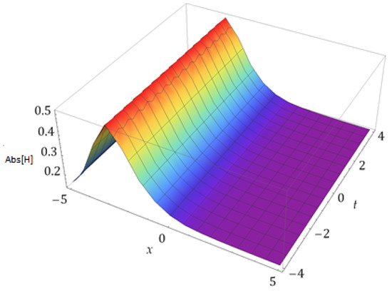
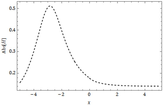
Figure 2. Plot for $H(x,y,z,w,t)$ appearance in Equation (31) in 2-dim for $t=1$.

Figure 3. Plot for $H(x,y,z,w,t)$ appearance in Equation (31) in 3-dim for the x–y plane.

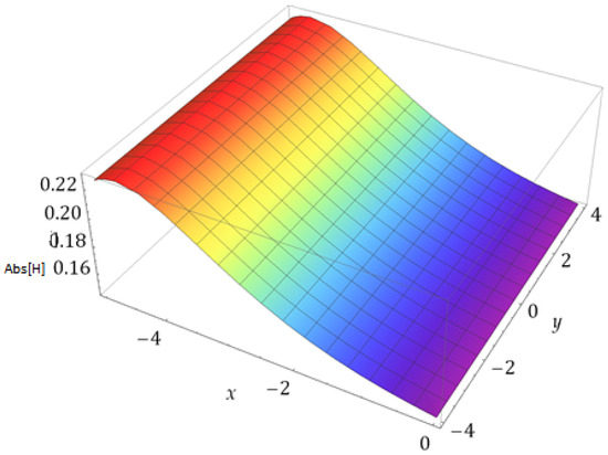
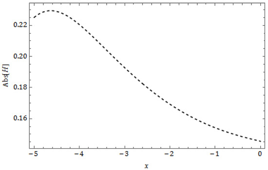
Figure 4. Plot for $H(x,y,z,w,t)$ appearance in Equation (31) in 2-dim for $y=1$.

Figure 5. Plot for $H(x,y,z,w,t)$ appearance in Equation (31) in 3-dim for the x–z plane.

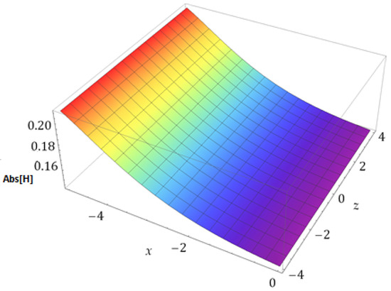
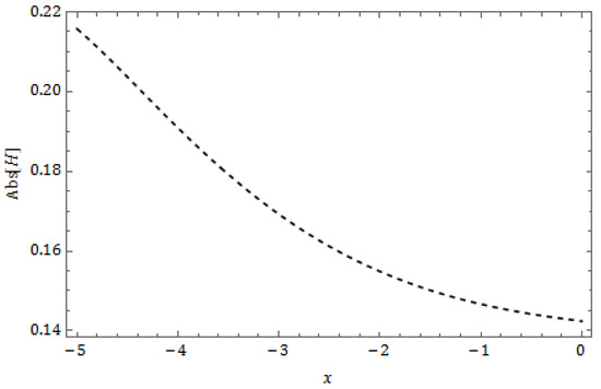
Figure 6. Plot for $H(x,y,z,w,t)$ appearance in Equation (31) in 2-dim for $z=1$.

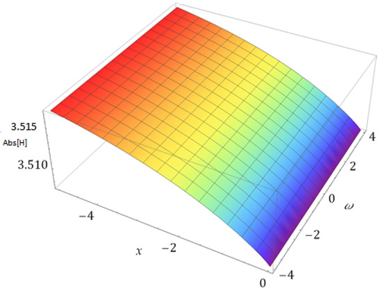
Figure 7. Plot for $H(x,y,z,w,t)$ appearance in Equation (31) in 3-dim for the x-$\omega$ plane.

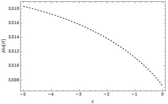
Figure 8. Plot for $H(x,y,z,w,t)$ appearance in Equation (31) in 2-dim for $w=1$.

Figure 9. Plot for $H(x,y,z,w,t)$ appearance in Equation (33) in 3-dim for the x–t plane.

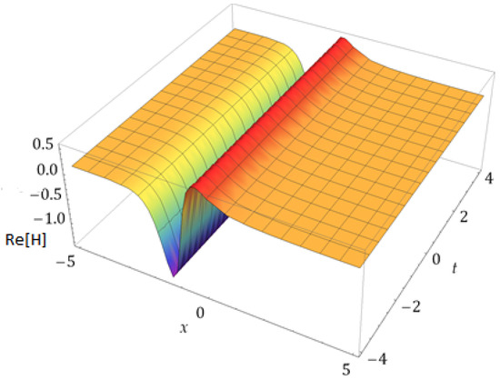
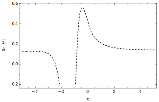
Figure 10. Plot for $H(x,y,z,w,t)$ appearance in Equation (33) in 2-dim for $t=1$.

Figure 11. Plot for $H(x,y,z,w,t)$ appearance in Equation (33) in 3-dim for the x–y plane.

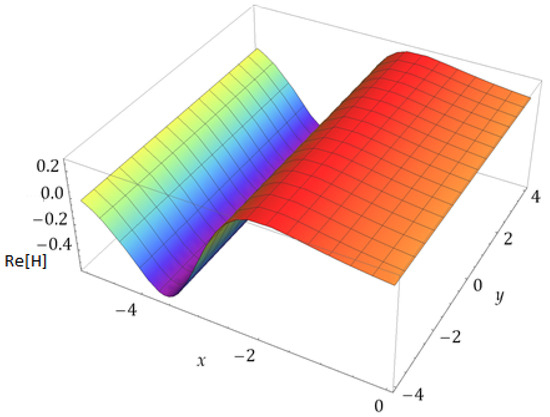
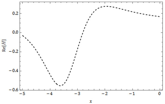
Figure 12. Plot for $H(x,y,z,w,t)$ appearance in Equation (33) in 2-dim for $y=1$.

Figure 13. Plot for $H(x,y,z,w,t)$ appearance in Equation (33) in 3-dim for the x–z plane.

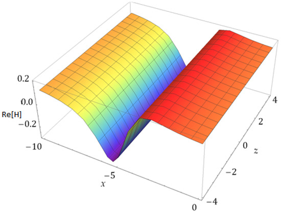
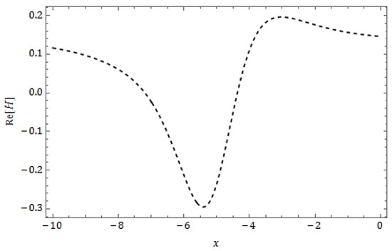
Figure 14. Plot for $H(x,y,z,w,t)$ appearance in Equation (33) in 2-dim for $z=1$.

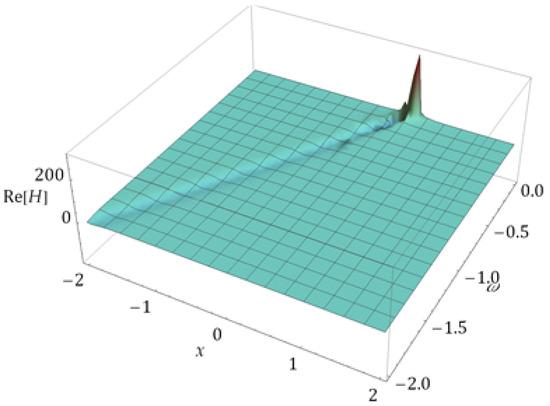
Figure 15. Plot for $H(x,y,z,w,t)$ appearance in Equation (33) in 3-dim for the x–$\omega$ plane.

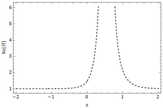
Figure 16. Plot for $H(x,y,z,w,t)$ appearance in Equation (33) in 2-dim for $w=1$.

Figure 17. Plot for $H(x,y,z,w,t)$ appearance in Equation (35) in 3-dim for the x–t plane.

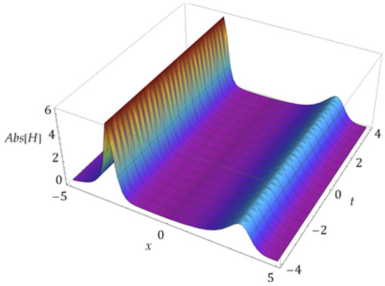
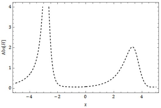
Figure 18. Plot for $H(x,y,z,w,t)$ appearance in Equation (35) in 2-dim for $t=1$.

Figure 19. Plot for $H(x,y,z,w,t)$ appearance in Equation (35) in 3-dim for the x–y plane.

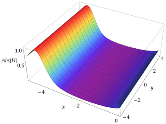
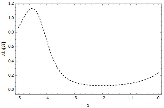
Figure 20. Plot for $H(x,y,z,w,t)$ appearance in Equation (35) in 2-dim for $y=1$.

Figure 21. Plot for $H(x,y,z,w,t)$ appearance in Equation (35) in 3-dim for the x–z plane.

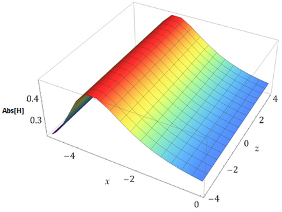
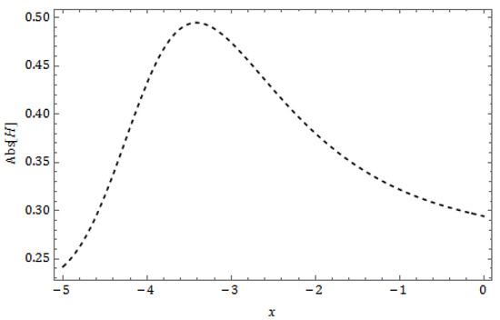
Figure 22. Plot for $H(x,y,z,w,t)$ appearance in Equation (35) in 2-dim for $z=1$.

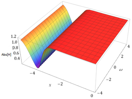
Figure 23. Plot for $H(x,y,z,w,t)$ appearance in Equation (35) in 3-dim for the x–$\omega$ plane.

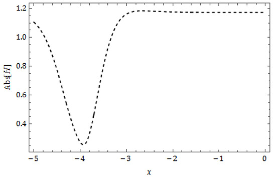
Figure 24. Plot for $H(x,y,z,w,t)$ appearance in Equation (35) in 2-dim for $w=1$.

Figure 25. Plot for $H(x,y,z,w,t)$ appearance in Equation (36) in 3-dim for the x–t plane.

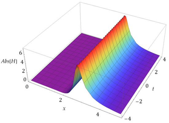
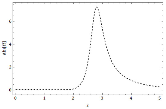
Figure 26. Plot for $H(x,y,z,w,t)$ appearance in Equation (36) in 2-dim for $t=1$.

Figure 27. Plot for $H(x,y,z,w,t)$ appearance in Equation (36) in 3-dim for the x–y plane.

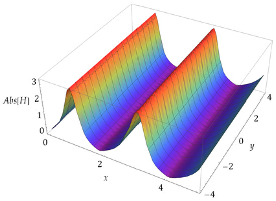
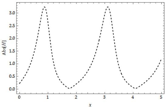
Figure 28. Plot for $H(x,y,z,w,t)$ appearance in Equation (36) in 2-dim for $y=1$.

Figure 29. Plot for $H(x,y,z,w,t)$ appearance in Equation (36) in 3-dim for the x–z plane.

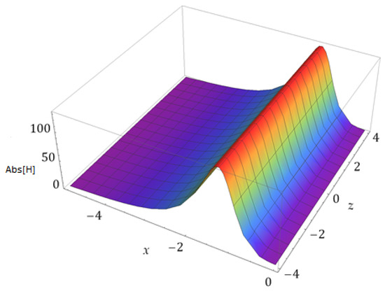
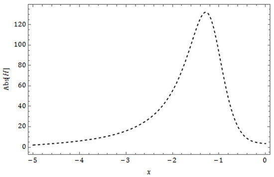
Figure 30. Plot for $H(x,y,z,w,t)$ appearance in Equation (36) in 2-dim for $z=1$.

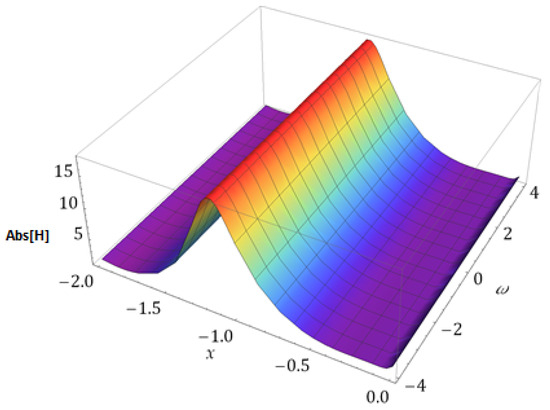
Figure 31. Plot for $H(x,y,z,w,t)$ appearance in Equation (36) in 3-dim for the x–$\omega$ plane.

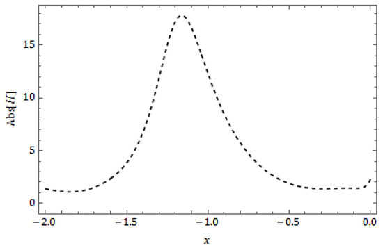
Figure 32. Plot for $H(x,y,z,w,t)$ appearance in Equation (36) in 2-dim for $w=1$.

Figure 33. Plot for $H(x,y,z,w,t)$ appearance in Equation (88) in 3-dim for the x–t plane.

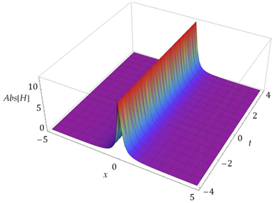
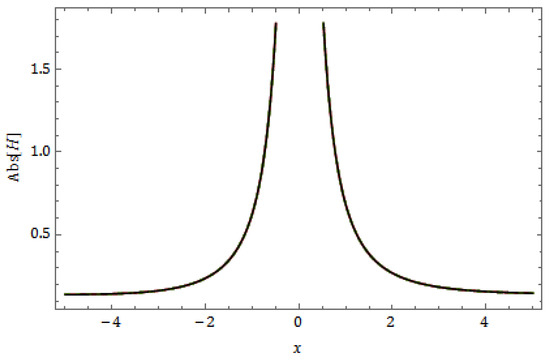
Figure 34. Plot for $H(x,y,z,w,t)$ appearance in Equation (88) in 2-dim for $t=1$.

Figure 35. Plot for $H(x,y,z,w,t)$ appearance in Equation (88) in 3-dim for the x–y plane.

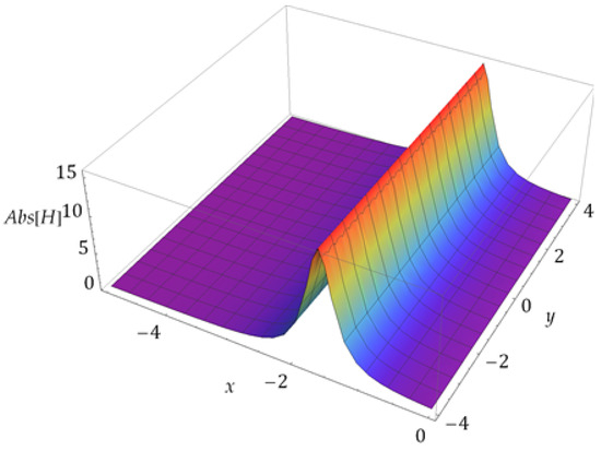
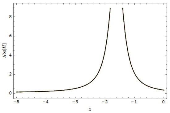
Figure 36. Plot for $H(x,y,z,w,t)$ appearance in Equation (88) in 2-dim for $y=1$.

Figure 37. Plot for $H(x,y,z,w,t)$ appearance in Equation (88) in 3-dim for the x–z plane.

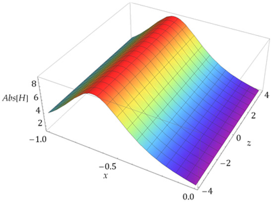
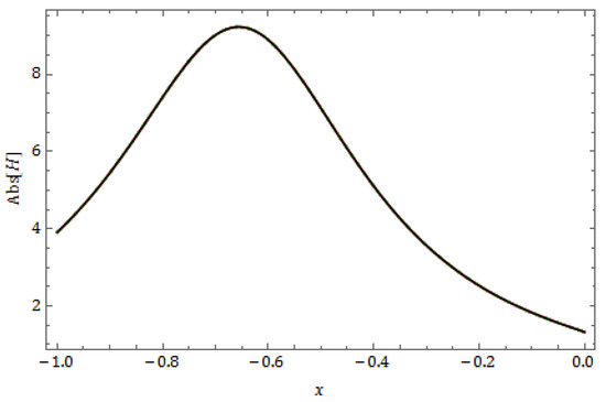
Figure 38. Plot for $H(x,y,z,w,t)$ appearance in Equation (88) in 2-dim for $z=1$.

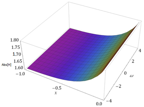
Figure 39. Plot for $H(x,y,z,w,t)$ appearance in Equation (88) in 3-dim for the x–$\omega$ plane.

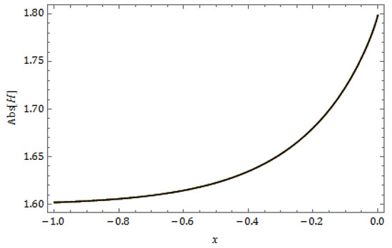
Figure 40. Plot for $H(x,y,z,w,t)$ appearance in Equation (88) in 2-dim for $w=1$.

Figure 41. Plot for $H(x,y,z,w,t)$ appearance in Equation (89) in 3-dim for the x–t plane.

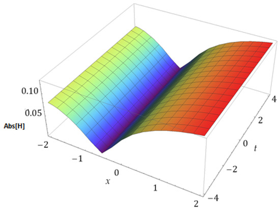
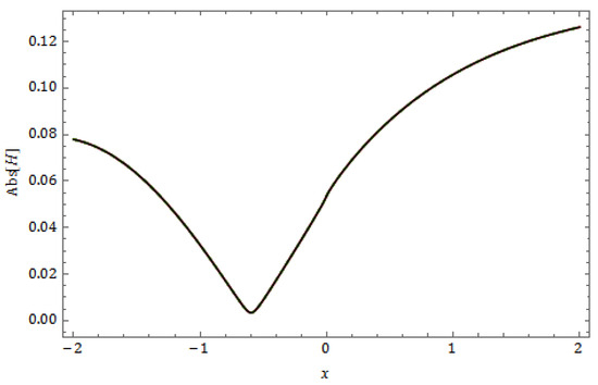
Figure 42. Plot for $H(x,y,z,w,t)$ appearance in Equation (89) in 2-dim for $t=1$.

Figure 43. Plot for $H(x,y,z,w,t)$ appearance in Equation (89) in 3-dim for the x–y plane.

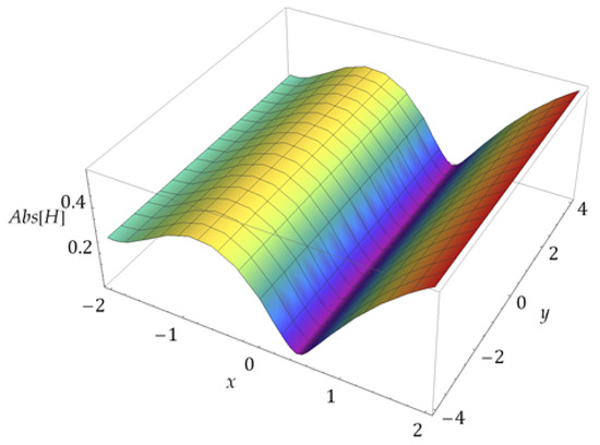
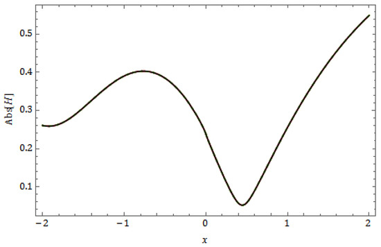
Figure 44. Plot for $H(x,y,z,w,t)$ appearance in Equation (89) in 2-dim for $y=1$.

Figure 45. Plot for $H(x,y,z,w,t)$ appearance in Equation (89) in 3-dim for the x–z plane.

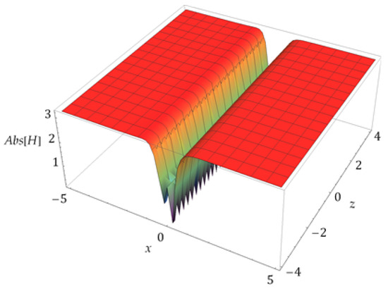
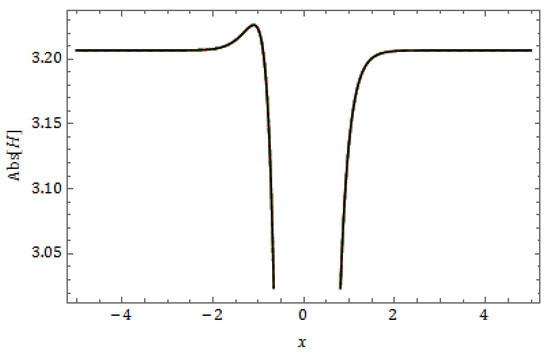
Figure 46. Plot for $H(x,y,z,w,t)$ appearance in Equation (89) in 2-dim for $z=1$.

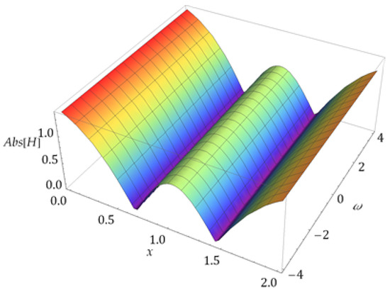
Figure 47. Plot for $H(x,y,z,w,t)$ appearance in Equation (89) in 3-dim for the x–$\omega$ plane.

Figure 48. Plot for $H(x,y,z,w,t)$ appearance in Equation (89) in 2-dim for $w=1$.

5. Conclusions

We have succeeded in attaining novel exact solitons to the nonlinear (4+1)-dimensional DSKP model with a truncated M-fractional derivative. For this purpose, we utilize the unified and modified extended tanh-expansion function techniques. The achieved solutions contained trigonometric, hyperbolic trigonometric, and exponential functions. Our results are newer and closer to the numerical solutions than the existing solutions of the model in the literature. Some of the obtained solutions are also represented by two-dimensional, three-dimensional, and contour graphs in the form of kink, singular, bright, periodic, and dark solitons. Fractional effects on solutions are also shown in graphs. Our solutions will be helpful in further study of the model concerned.

References

- Akter, S.; Hossain, M.D.; Uddin, M.F.; Hafez, M.G. Collisional Solitons Described by Two-Sided Beta Time Fractional Korteweg-de Vries Equations in Fluid-Filled Elastic Tubes. Adv. Math. Phys. 2023, 2023, 9594339. [Google Scholar] [CrossRef]
- Uddin, M.F.; Hafez, M.G.; Hwang, I.; Park, C. Effect of space fractional parameter on nonlinear ion acoustic shock wave excitation in an unmagnetized relativistic plasma. Front. Phys. 2022, 9, 766. [Google Scholar] [CrossRef]
- Hafez, M.G.; Iqbal, S.A.; Akther, S.; Uddin, M.F. Oblique plane waves with bifurcation behaviors and chaotic motion for resonant nonlinear Schrodinger equations having fractional temporal evolution. Results Phys. 2019, 15, 102778. [Google Scholar] [CrossRef]
- Uddin, M.F.; Hafez, M.G.; Hammouch, Z.; Rezazadeh, H.; Baleanu, D. Traveling wave with beta derivative spatial-temporal evolution for describing the nonlinear directional couplers with metamaterials via two distinct methods. Alex. Eng. J. 2021, 60, 1055–1065. [Google Scholar] [CrossRef]
- Uddin, M.F.; Hafez, M.G. Interaction of complex short wave envelope and real long wave described by the coupled Schrödinger–Boussinesq equation with variable coefficients and beta space fractional evolution. Results Phys. 2020, 19, 103268. [Google Scholar] [CrossRef]
- Uddin, M.F.; Hafez, M.G.; Iqbal, S.A. Dynamical plane wave solutions for the Heisenberg model of ferromagnetic spin chains with beta derivative evolution and obliqueness. Heliyon 2022, 8, e09199. [Google Scholar] [CrossRef] [PubMed]
- Uddin, M.F.; Hafez, M.G. Optical Wave Phenomena in Birefringent Fibers Described by Space-Time Fractional Cubic-Quartic Nonlinear Schrödinger Equation with the Sense of Beta and Conformable Derivative. Adv. Math. Phys. 2022, 2022, 7265164. [Google Scholar] [CrossRef]
- Ahmad, I.; Jalil, A.; Ullah, A.; Ahmad, S.; De la Sen, M. Some new exact solutions of (4+1)-dimensional Davey–Stewartson-Kadomtsev–Petviashvili equation. Results Phys. 2023, 45, 106240. [Google Scholar] [CrossRef]
- Sulaiman, T.A.; Yel, G.; Bulut, H. M-fractional solitons and periodic wave solutions to the Hirota-Maccari system. Mod. Phys. Lett. B 2019, 33, 1950052. [Google Scholar] [CrossRef]
- Sousa, J.V.d.A.C.; Capelas de Oliveira, E. A new truncated M-fractional derivative type unifying some fractional derivative types with classical properties. Int. J. Anal. Appl. 2018, 16, 83–96. [Google Scholar]
- Fokas, A.S. Integrable nonlinear evolution partial differential equations in 4+2 and 3+1 dimensions. Phys. Rev. Lett. 2006, 96, 190201. [Google Scholar] [CrossRef] [PubMed]
- Akbar, M.A.; Abdullah, F.A.; Gepreel, K.A. The solitonic solutions of finite depth long water wave models. Results Phys. 2022, 37, 105570. [Google Scholar] [CrossRef]
- Talafha, A.M.; Jhangeer, A.; Kazmi, S.S. Dynamical analysis of (4+1)-dimensional Davey Srewartson Kadomtsev Petviashvili equation by employing Lie symmetry approach. Ain Shams Eng. J. 2023, 14, 102537. [Google Scholar] [CrossRef]
- El-Shorbagy, M.A.; Akram, S.; Rahman, M.u. Propagation of solitary wave solutions to (4+1)-dimensional Davey–Stewartson–Kadomtsev–Petviashvili equation arise in mathematical physics and stability analysis. Partial. Differ. Equ. Appl. Math. 2024, 10, 100669. [Google Scholar] [CrossRef]
- Ahmad, S.; Ullah, A.; Ahmad, S.; Saifullah, S.; Shokri, A. Periodic solitons of Davey Stewartson Kadomtsev Petviashvili equation in (4+1)-dimension. Results Phys. 2023, 50, 106547. [Google Scholar] [CrossRef]
- Junjua, M.D.; Mostafa, A.M.; AlQahtani, N.F.; Bekir, A. Impact of truncated M-fractional derivative on the new types of exact solitons to the (4+1)-dimensional DSKP model. Mod. Phys. Lett. B 2024, 2024, 2450313. [Google Scholar] [CrossRef]
- Ullah, M.S.; Abdeljabbar, A.; Roshid, H.O.; Ali, M.Z. Application of the unified method to solve the Biswas—Arshed model. Results Phys. 2022, 42, 105946. [Google Scholar] [CrossRef]
- Nandi, D.C.; Ullah, M.S.; Ali, M.Z. Application of the unified method to solve the ion sound and Langmuir waves model. Heliyon 2022, 8, e10924. [Google Scholar] [CrossRef] [PubMed]
- Wang, X.; Javed, S.A.; Majeed, A.; Kamran, M.; Abbas, M. Investigation of exact solutions of nonlinear evolution equations using unified method. Mathematics 2022, 10, 2996. [Google Scholar] [CrossRef]
- Shahen, N.H.M.; Rahman, M.M. Dispersive solitary wave structures with MI Analysis to the unidirectional DGH equation via the unified method. Partial. Differ. Equ. Appl. Math. 2022, 6, 100444. [Google Scholar]
- Alam, L.M.B.; Jiang, X. Exact and explicit traveling wave solution to the time-fractional phi-four and (2+1) dimensional CBS equations using the modified extended tanh-function method in mathematical physics. Partial. Differ. Equ. Appl. Math. 2021, 4, 100039. [Google Scholar] [CrossRef]
- Zahran, E.H.M.; Khater, M.M.A. Modified extended tanh-function method and its applications to the Bogoyavlenskii equation. Appl. Math. Model. 2016, 40, 1769–1775. [Google Scholar] [CrossRef]
- Raslan, K.R.; Ali, K.K.; Shallal, M.A. The modified extended tanh method with the Riccati equation for solving the space-time fractional EW and MEW equations, Chaos. Solitons Fractals 2017, 103, 404–409. [Google Scholar] [CrossRef]
Disclaimer/Publisher’s Note: The statements, opinions and data contained in all publications are solely those of the individual author(s) and contributor(s) and not of MDPI and/or the editor(s). MDPI and/or the editor(s) disclaim responsibility for any injury to people or property resulting from any ideas, methods, instructions or products referred to in the content. |
© 2024 by the authors. Licensee MDPI, Basel, Switzerland. This article is an open access article distributed under the terms and conditions of the Creative Commons Attribution (CC BY) license (https://creativecommons.org/licenses/by/4.0/).