Fractional Second-Grade Fluid Flow over a Semi-Infinite Plate by Constructing the Absorbing Boundary Condition

Abstract

The modified second-grade fluid flow across a plate of semi-infinite extent, which is initiated by the plate’s movement, is considered herein. The relaxation parameters and fractional parameters are introduced to express the generalized constitutive relation. A convolution-based absorbing boundary condition (ABC) is developed based on the artificial boundary method (ABM), addressing issues related to the semi-infinite boundary. We adopt the finite difference method (FDM) for deriving the numerical solution by employing the L1 scheme to approximate the fractional derivative. To confirm the precision of this method, a source term is added to establish an exact solution for verification purposes. A comparative evaluation of the ABC versus the direct truncated boundary condition (DTBC) is conducted, with their effectiveness and soundness being visually scrutinized and assessed. This study investigates the impact of the motion of plates at different fluid flow velocities, focusing on the effects of dynamic elements influencing flow mechanisms and velocity. This research’s primary conclusion is that a higher fractional parameter correlates with the fluid flow. As relaxation parameters decrease, the delay effect intensifies and the fluid velocity decreases.

1. Introduction

Viscoelastic fluid is widely used in petroleum exploitation, medicine, biology, and other fields [1,2,3]. Viscoelastic fluid combines the viscosity of the fluid and the elasticity of the elastic solid, which shows the complex behavior between them and makes it a typical non-Newtonian fluid. Viscoelastic fluid has a time-dependent stress–strain response, showing shear rate-dependent viscosity and elastic recovery after unloading. Second-grade fluids are a specialized subclass of non-Newtonian fluids [4,5] which exhibit unique viscoelastic characteristics. A feature of these fluids is that their velocity field includes two derivatives within the correlation linking stress to strain, whereas the velocity field of Newtonian fluid contains only a first-order derivative. To better understand the flow characteristics of second-grade fluids, scholars often choose a simple model for analysis, which is helpful to understand the motion nature of second-grade fluid more deeply and provide theoretical support for related industrial applications. Ho et al. [6] investigated the migration of rigid spheres in a flowing second-grade fluid by simplifying the fluid flow problem between parallel plane walls. Khan et al. [7] gave an exact analytical solution for the fluid flow of a generalized second-grade fluid between two walls perpendicular to a flat plate. Tassaddiq [8] analyzed the flow of a second-grade fluid by simplifying the problem to a non-constant flow of the incompressible fluid over an inclined plate with an inclined magnetic field. Further studies are cited in references [9,10]. This paper focuses on the behavior of generalized second-grade fluids over a semi-infinite plate which contains broad applications in various fields, as noted in references [11,12,13,14], including the flow of biological fluids, liquid metals and alloys, plasma, and blood.

The traditional second-grade fluid constitutive relation is grounded in integer differentials [15,16]. By considering the historical memory during their flow process, meaning that their current state is not solely determined by the present stress state but is also influenced by the stress history of the past, the fractional second-grade fluid is developed. The fractional differential equations [17,18,19,20] surpass the capabilities of integer-based models and offer a more precise capture of the historical dependency. Furthermore, the fractional derivatives possess a nonlocal nature; the derivative value at any given instant is intimately connected to the entire historical trajectory. This attribute equips fractional differential equations with the ability to describe physical processes exhibiting long-range or spatially extensive correlations [21]. The fractional operator addresses the significant inconsistencies between classical integer differential models and experimental outcomes, which compensates for their serious shortcomings. Consequently, it can achieve superior fitting results with experimental data by utilizing a reduced number of parameters. Sene et al. [22] used the double integration method to solve the fractional differential equation in the two-level fluid model. Chan et al. [23] carried out research into the behavior of deformable droplets when suspended within a second-grade fluid environment. Jiang et al. [24] made contributions to the field by examining the unsteady magnetohydrodynamic flow of a modified second-grade fluid by taking into account the Hall effect, as it pertains to movement through porous media. For more research on fractional derivatives in the field of viscoelastic fluids, the readers are encouraged to refer to [25,26,27]. In this work, we integrate the fundamental equation governing fluid dynamics with a model representing a modified second-grade fluid which includes the application of Riemann–Liouville time fractional derivative (RLTFD) operators.

Numerical simulations, when analyzing flow mechanisms, can demonstrate the flow properties of complex fluid models, eliminating the necessity of experimental procedures. Within this study, the formulation of the equation is achieved through the application of the FDM, as introduced in references [28,29]. The FDM is a numerical technique that divides a continuous domain into discrete grids and approximates the equation at these grid points. This method is adept at transforming a partial differential equation into a collection of either linear or nonlinear algebraic equation. This conversion facilitates straightforward numerical solutions that can be efficiently computed with the aid of computer systems. The FDM is not only intuitive in concept and easy to implement in programming, but also can flexibly handle problems with various boundary conditions and complex geometric shapes. Mei et al. [30] studied the flow around a sphere with free flow velocity oscillation and unsteady resistance under a finite Reynolds number by using FDM. Dennis et al. [31] proposed a new FDM for calculating steady flow in curved pipes. Kim et al. [32] developed a computational approach specifically tailored for the second-grade gradient theory of incompressible fluid dynamics. For more related research, one can refer to [33,34,35]. In addition, in the numerical simulation of the fractional derivatives, a variety of interpolation approximation methods has been reported, such as Grünwald–Letnikov definition [36], the L1 scheme [37], the $\mathrm{L}2-1_{\sigma }$ scheme [38] and the fast algorithm [39].

The critical challenge in numerical methods pertains to the effective reduction of the effects that the unbounded regions exert on computational outcomes. Historically, the prevalent approach to dealing with the unbounded regions is through the employment of a direct truncation method (DTM), as documented in reference [40]. This approach involves selecting an exceedingly large value at the boundary, rather than attempting to define an actual infinite boundary condition. The DTM is less favorable for performing computer-based numerical simulations, notably for those that are extended over a long duration. In this paper, we employ an alternative strategy referred to as the artificial boundary method to establish the ABC. The core concept of this approach entails partitioning the unbounded domain into two distinct regions: a confined computational zone, which is the internal area, and an unbounded zone, representing the external area. The chosen boundary points need to ensure that the source term is compactly supported within a finite truncation area. Subsequently, the relation at the truncation point is determined through the use of the Laplace transform in the external region. The use of this approach retains the effect exerted by the external area on the truncated boundary, which ensures the restricted area has a more reasonable boundary condition. The mentioned approach has been utilized extensively in various studies. For instance, Barucq et al. [41] analyzed the Helmholtz equation numerically by using ABC. They conducted an in-depth analysis of the impact of various parameters on these numerical results. Li et al. [42] solved the effective second-grade Schrödinger equation with the FDM by constructing ABCs. Muhr et al. [43] applied the ABC to address the Westervelt wave equation related to sound velocity potential, and the effectiveness and efficiency were confirmed. Further information on ABC is available in [44,45,46].

This paper studies the impulsive motion of a modified second-grade fluid on a plate of semi-infinite extent by introducing an ABC. In Section 2, we propose the constitutive relation and formulate the governing equation. Section 3 details the development and construction of the ABC. In Section 4, the numerical framework for the governing equation, along with its initial and boundary conditions (IBCs), is presented. In Section 5, four numerical instances are provided, detailing numerical methods’ efficacy, the dynamic parameters’ impacts on velocity, the ABC, and a comparison of this study with other methods. Section 6 offers a summary of these findings.

2. The Construction of the Governing Equation

We are now focusing on an infinitely extended flat plate with a fluid situated on a single side of the plate. In the initial state, the plate and the fluid above it remain stationary. Suddenly, the flat plate initiates movement with a velocity denoted as $u_w(t)$. As Figure 1 shows, we use a coordinate system where the flow progresses in the $x$ direction, while the $y$ direction is perpendicular to the plate. The positions of the plate are denoted as $y=0$. The fluid’s velocity on the surface of the plate is equal to the plate’s velocity, which considers the no-slip condition. The fluid is regarded as a generalized second-grade fluid with stresses that depend not only on the current strain rate, but also possibly on the historical one. We neglect sidewall effects because the plate is considered to be infinitely long, such that the flow problem is mainly controlled by the motion of the plate and the viscoelastic properties of the fluid. In addition, the fluid is considered incompressible. The flow is supposed to be laminar, and no turbulence occurs. Finally, the deformation of the fluid is small and can be analyzed using linear theory. Collectively, these stipulations and suppositions constitute the foundational framework upon which the problem’s analysis and resolution are predicated.

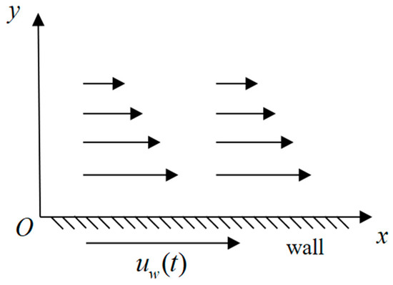
Figure 1. Schematic diagram of fractional second-grade fluid flow problem on a plate of semi-infinite extent.

The constitutive relation for a second-grade fluid satisfies [45]:

$$T=-pI+\mu A_1+{\alpha }_1{A}_2+{\alpha }_2{A_1}^2$$

(1)

in which the identity tensor is expressed as $I$, the hydrostatic pressure is expressed as $p$, the stress tensor is expressed as $T$, $\mu$ represents the coefficients of viscosity, ${\alpha }_1$ and ${\alpha }_2$ denote as the normal stress moduli, and the symbols $A_1$ and $A_2$ refer to the kinematic tensors [47] separately described by the following equation.

$$A_1=\nabla V+{\left(\nabla V\right)}^{\mathrm{T}}$$

(2)

$$A_2=\frac{\partial A_1}{\partial t}+A_1(\nabla V)+{\left(\nabla V\right)}^{\mathrm{T}}{A}_1$$

(3)

in which $\frac{\partial }{\partial t}$ is indicative of the material time partial derivative, $V$ expresses the velocity vector field, and $\nabla$ is the operator of the gradient. Suppose that the fluid described by Equation (1) conforms to thermodynamics, then all motions of the fluid satisfy the Clausius–Duhem inequality. Assume that the specific Helmholtz free energy of the fluid is minimized when the fluid is locally stationary [48]; then,

$$\mu ⩾0, {\alpha }_1⩾0, {\alpha }_1+{\alpha }_2=0$$

(4)

The fractional derivatives are able to describe the nonlocality and memory effects [17,21] of the generalized second-grade fluid. Since the fractional derivatives are nonlocal, this allows fractional differential equations to describe physical processes with long-range correlations or spatial-extent correlations. In general, the constitutive relation for the fractional second-grade fluid [49,50] also assumes the form (1), yet $A_2$ satisfies

$$A_2={}_0{}^{RL}\mathcal{D}_t^{\beta }{A}_1+A_1(\nabla V)+{(\nabla V)}^{\mathrm{T}}{A}_1$$

(5)

in which ${}_0{}^{RL}\mathcal{D}_t^{\beta }$ denotes the RLTFD operator [51].

The RLTFD operator ${}_0{}^{RL}\mathcal{D}_t^{\beta }$ satisfies

$${}_0{}^{RL}\mathcal{D}_t^{\beta }u(y,t)=\frac{\partial }{\partial t}\left(\frac{1}{\Gamma \left(1-\beta \right)}{\displaystyle {\int }_0^t\frac{u(y,\tau )d\tau }{{\left(t-\tau \right)}^{\beta }}}\right), 0<\beta <1$$

(6)

where $\Gamma (\cdot )$ denotes the Gamma function. When $\beta =1$, using the RLTFD’s property, one obtains ${}_0{}^{RL}\mathcal{D}_t^{\beta }f(t)={}_0{}^{RL}\mathcal{D}_t^1\left({}_0{}^{RL}\mathcal{D}_t^{0}f(t)\right)=\frac{\mathrm{d}f(t)}{\mathrm{d}t}$, namely, Equation (5) simplifies to Equation (3). When ${\alpha }_1=0$ and ${\alpha }_2=0$, the classical viscous Newtonian fluid is recovered [52,53]. It should be indicated that we have kept the same notation for the constant ${\alpha }_1$ in (1) for the sake of simplicity, but it refers to a new material constant with the dimensions $kg\cdot m^{-1}\cdot s^{\beta -1}$. It reduces to $kg\cdot m^{-1}$ for $\beta \to 1$. For the other relations between (1) and (3), they remain formally unchanged under the above dimensional understanding [54].

Neglecting the external forces, the equation of motion satisfies

$$\rho \frac{\mathrm{D}V}{\mathrm{D}t}=\nabla \cdot T$$

(7)

in which the fluid’s density is expressed as $\rho$, and the material derivative is represented as $\frac{\mathrm{D}}{\mathrm{D}t}$.

The continuity equation for velocity is expressed as

$$\nabla \cdot V=0$$

(8)

Consider a modified second-grade fluid flowing close to a plate, moving with the velocity $u_w(t)$ within its own plane suddenly. The $x$-axis is defined following the motion adjacent to the wall, and the $y$-axis and the wall are perpendicular. Assuming the effects of the side walls can be disregarded and implying the wall is infinitely long, we aim to find solutions in the form of the velocity field as

$$V=u(y,t)i$$

(9)

in which the $x$-direction unit vector is represented as $i$, and the $x$-direction velocity is expressed as $u$.

The stresses exerted on the plate initiate the movement of the fluid, which is given by (1), (2), (4), and (5). Substituting (9) into (1)–(6), we obtain

$$T_{xy}=\mu \frac{\partial u}{\partial y}+{\alpha }_1{}_0{}^{RL}\mathcal{D}_t^{\beta }\frac{\partial u}{\partial y}$$

(10)

where $T_{xy}=T_{yx}$ and $T_{xx}=T_{yy}=T_{zz}=T_{xz}=T_{yz}=0$. Note that we have kept the same notation for the constant ${\alpha }_1$ in (10), but it refers to a new material constant with the dimensions $kg\cdot m^{-1}\cdot s^{\beta -1}$.

By introducing (9) and (10) into (7), it yields

$$\rho \frac{\partial u}{\partial t}=\mu \frac{{\partial }^{2}u}{\partial y^2}+{\alpha }_1{}_0{}^{RL}\mathcal{D}_t^{\beta }\frac{{\partial }^{2}u}{\partial y^2}$$

(11)

The IBCs satisfy

$$u(y,0)=0, y>0$$

(12)

$$u\left(0,t\right)=u_w\left(t\right), u\left(+\infty ,t\right)=0, t\in \left[0,T\right]$$

(13)

where $u_w\left(t\right)$ is the velocity of the plate.

Dimensionless variables are introduced to facilitate the analysis

$$\stackrel{⌢}{u}=\frac{u}{U}, \stackrel{⌢}{y}=\frac{yU\rho }{\mu }, \stackrel{⌢}{t}=\frac{t{U}^2\rho }{\mu }, {\stackrel{⌢}{u}}_w(\stackrel{⌢}{t})=\frac{u_w(t)}{U}$$

(14)

where $U$ represents the characteristic velocity.

For generalization purposes, the form of $f\left(y,t\right)$ is presented. Subsequently, the dimensionless governing equation along with its IBCs are presented as follows (the superscript “$\stackrel{⏜}{ }$” is omitted)

$$\frac{\partial u(y,t)}{\partial t}=\frac{{\partial }^{2}u(y,t)}{\partial y^2}+\eta {}_0{}^{RL}\mathcal{D}_t^{\beta }\frac{{\partial }^{2}u(y,t)}{\partial y^2}+f\left(y,t\right)$$

(15)

$$u(y,0)=0, y>0$$

(16)

$$u\left(0,t\right)=u_w(t), u\left(+\infty ,t\right)=0, t\in \left[0,T\right]$$

(17)

where $\eta =\frac{{\alpha }_1{U}^{2\beta }{\rho }^{\beta }}{{\mu }^{\beta +1}}$.

3. The Establishment of the ABC

By using the ABM, we formulate the exact ABC. First, the unbounded region $\Omega :=\left\{y\left|0\le y<+\infty \right.\right\}$ is truncated by the point $y_r$. In such a case, we divide the unbounded region as the unbounded area ${\Omega }_r:=\left\{y\left|y_r\le y<+\infty \right.\right\}$ located to the right, and the bounded area ${\Omega }_c:=\left\{y\left|0\le y\le y_r\right.\right\}$ is designated for calculation. The selection of $y_r$ demands that the initial conditions and the source term be compactly supported in region ${\Omega }_c$.

In the unbounded region ${\Omega }_r$, we have

$$\frac{\partial u\left(y,t\right)}{\partial t}=\frac{{\partial }^{2}u\left(y,t\right)}{\partial y^2}+\eta {}_0{}^{RL}\mathcal{D}_t^{\beta }\frac{{\partial }^{2}u\left(y,t\right)}{\partial y^2}+f\left(y,t\right)$$

(18)

$$u(y,0)=0 \mathrm{for} y>0$$

(19)

$$u\left(+\infty ,t\right)=0 \mathrm{when} t\in \left[0,T\right]$$

(20)

Since $\beta$ is between zero and one, the Laplace transform for ${}_0{}^{RL}\mathcal{D}_t^{\beta }$ [55] has the form $L\left\{{}_0{}^{RL}\mathcal{D}_t^{\beta }f(t),s\right\}=s^{\beta }L\left\{f(t),s\right\}-{\left[{}_0{}^{RL}\mathcal{D}_t^{\beta -1}f(t)\right]}_{t=0}$. By referring to the principle of the Laplace transform for the RLTFD, we obtain

$$\frac{{\partial }^2\widehat{u}\left(y,s\right)}{\partial y^2}-\frac{s}{1+\eta s^{\beta }}\widehat{u}\left(y,s\right)=0$$

(21)

in which the Laplace transform of $u\left(y,t\right)$ is represented as $\widehat{u}\left(y,s\right)$.

Solving the above equation yields

$$\widehat{u}\left(y,s\right)=e^{-\sqrt{\frac{s}{1+\eta s^{\beta }}}y}$$

(22)

For Equation (22), we take the derivative for $y$

$$\frac{\partial \widehat{u}\left(y,s\right)}{\partial y}=-\frac{1}{{\left(1+\eta s^{\beta }\right)}^{\frac{1}{2}}}\widehat{u}\left(y,s\right)$$

(23)

Before performing the inverse Laplace transform, it is crucial to define the generalized Mittag–Leffler function [55]:

$$E_{k,l}^{\gamma }\left(z\right)={\displaystyle \sum _{n=0}^{\infty }\frac{{\left(\gamma \right)}_n}{n!\Gamma \left(nk+l\right)}{z}^n}, \mathrm{Re}k>0, l\in C, \gamma >0$$

(24)

where ${\left(\gamma \right)}_n=\gamma \left(\gamma +1\right)\cdots \left(\gamma +n-1\right)=\Gamma \left(\gamma +n\right)/\Gamma \left(\gamma \right)$.

The Mittag–Leffler function [55] has the following property:

$$\mathcal{L}\left\{t^{l-1}{E}_{k,l}^{\gamma }\left(-\lambda t^k\right),s\right\}=\frac{s^{k\gamma -l}}{{\left(\lambda +s^k\right)}^{\gamma }}$$

(25)

where $\mathrm{Re}k>0$ and $\mathrm{Re}l>0$.

By conducting the inverse Laplace transformation for (23), we infer the ABC at $y=y_r$

$$\frac{\partial u(y_r,t)}{\partial y}=-\sqrt{\frac{1}{\eta }}\left[t^{\frac{1}{2}\beta -1}{E}_{\beta ,\frac{1}{2}\beta }^{\frac{1}{2}}\left(-\frac{1}{\eta }{t}^{\beta }\right)\right]\ast {}_0{}^{RL}\mathcal{D}_t^{\frac{1}{2}}u(y_r,t)$$

(26)

where $\ast$ stands for the convolution.

To facilitate explanation, we introduce the notation as

$$K_1(t)=\sqrt{\frac{1}{\eta }}\left[t^{\frac{1}{2}\beta -1}{E}_{\beta ,\frac{1}{2}\beta }^{\frac{1}{2}}\left(-\frac{1}{\eta }{t}^{\beta }\right)\right]$$

(27)

After introducing the symbol $K_1(t)$, the Equation (26) changes:

$$\frac{\partial u(y_r,t)}{\partial y}={\displaystyle {\int }_0^t-K_1(t-\tau )\ast {}_0{}^{RL}\mathcal{D}_{\tau }^{\frac{1}{2}}u(y_r,\tau )}d\tau$$

(28)

Taking Equation (28) as the exact ABC, we formulate the governing equation based on the IBCs:

$$\frac{\partial u\left(y,t\right)}{\partial t}=\frac{{\partial }^{2}u\left(y,t\right)}{\partial y^2}+\eta {}_0{}^{RL}\mathcal{D}_t^{\beta }\frac{{\partial }^{2}u\left(y,t\right)}{\partial y^2}+f\left(y,t\right)$$

(29)

$$u(y,0)=0$$

(30)

$$u(0,t)=0$$

(31)

$$\frac{\partial u(y_r,t)}{\partial y}={\displaystyle {\int }_0^t-K_1(t-\tau )\ast {}_0{}^{RL}\mathcal{D}_{\tau }^{\frac{1}{2}}u(y_r,\tau )}d\tau$$

(32)

Now, we discuss the well-posedness of the considered problem. Since the initial condition of our question is zero, ${}_0{}^{RL}\mathcal{D}_t^{\beta }u(t)$ and ${}_0{}^C\mathcal{D}_t^{\beta }u(t)$ are equivalent. Then, the property for the Caputo fractional derivative is also applicable to the RLTFD. Initially, we introduce the following lemma.

Lemma 1. 

Assume $u(t)$ to be an absolutely continuous function on $\left[0,T\right]$. Considering $0<\beta <1$ and $u(0)=0$, it yields [56]

$$u(t){}_0{}^{RL}\mathcal{D}_t^{\beta }u(t)\ge \frac{1}{2}{}_0{}^{RL}\mathcal{D}_t^{\beta }{u}^2(t)$$

(33)

Theorem 1. 

The problem (29)–(32) is $L^2$ -stable and adheres to the subsequent estimation:

$${‖\frac{\partial u\left(y,t\right)}{\partial y}‖}_{L^2\left[0,y_r\right]}^2\le {‖f\left(y,t\right)‖}_{L^2\left[0,y_r\right]}^2$$

(34)

 where ${‖u\left(y,t\right)‖}_{L^2\left[a,b\right]}^2(t)={\displaystyle {\int }_a^b{\left|u\left(y,t\right)\right|}^2\mathrm{d}y}$.

Proof. 

In the outer region $\left(y_r,+\infty \right]$, the source term becomes zero due to the compactly supported assumption in $\left[0,y_r\right]$. Multiplying both sides of Equation (29) simultaneously by $\frac{{\partial }^{2}u\left(y,t\right)}{\partial y^2}$ and integrating over $y$ from $y_r$ to $+\infty$ and $t$ from 0 to $T$, it yields:

$$\begin{array}{l}{\displaystyle {\int }_0^T{\displaystyle {\int }_{y_r}^{+\infty }\frac{\partial u\left(y,t\right)}{\partial t}\frac{{\partial }^{2}w\left(y,t\right)}{\partial y^2}\mathrm{d}y}\mathrm{d}t}={\displaystyle {\int }_0^T{\displaystyle {\int }_{y_r}^{+\infty }\frac{{\partial }^{2}u\left(y,t\right)}{\partial y^2}\frac{{\partial }^{2}u\left(y,t\right)}{\partial y^2}\mathrm{d}y}\mathrm{d}t}\\ +\eta {\displaystyle {\int }_0^T{\displaystyle {\int }_{y_r}^{+\infty }\frac{{\partial }^{2}u\left(y,t\right)}{\partial y^2}{}_0{}^{RL}\mathcal{D}_t^{\beta }\frac{{\partial }^{2}u\left(y,t\right)}{\partial y^2}\mathrm{d}y}\mathrm{d}t}.\end{array}$$

(35)

Employing the method of integration by parts and Lemma 1 yields:

$${\displaystyle {\int }_0^T{\displaystyle {\int }_{y_r}^{+\infty }\frac{\partial u\left(y,t\right)}{\partial t}\frac{{\partial }^{2}u\left(y,t\right)}{\partial y^2}\mathrm{d}y}\mathrm{d}t}=-{\displaystyle {\int }_0^T\frac{\partial u\left(y_r,t\right)}{\partial t}\frac{\partial u\left(y_r,t\right)}{\partial y}\mathrm{d}t}-\frac{1}{2}{\displaystyle {\int }_0^T\frac{\partial }{\partial t}{‖\frac{\partial u\left(y,t\right)}{\partial y}‖}_{L^2\left(y_r,+\infty \right]}^2\mathrm{d}t}$$

(36)

Considering (30) and (31), we have:

$$\begin{array}{l}-{\displaystyle {\int }_0^T\frac{\partial u\left(y_r,t\right)}{\partial t}\frac{\partial u\left(y_r,t\right)}{\partial y}\mathrm{d}t}-\frac{1}{2}{\displaystyle {\int }_0^T\frac{\partial }{\partial t}{‖\frac{\partial u\left(y,t\right)}{\partial y}‖}_{L^2\left(y_r,+\infty \right]}^2\mathrm{d}t}\\ =-{\displaystyle {\int }_0^T\frac{\partial u\left(y_r,t\right)}{\partial t}\frac{\partial u\left(y_r,t\right)}{\partial y}\mathrm{d}t}-\frac{1}{2}{‖\frac{\partial u\left(y,T\right)}{\partial y}‖}_{L^2\left(y_r,+\infty \right]}^2\\ \le -{\displaystyle {\int }_0^T\frac{\partial u\left(y_r,t\right)}{\partial t}\frac{\partial u\left(y_r,t\right)}{\partial y}\mathrm{d}t}.\end{array}$$

(37)

The second term satisfies that:

$${\displaystyle {\int }_0^T{\displaystyle {\int }_{y_r}^{+\infty }\frac{{\partial }^{2}u\left(y,t\right)}{\partial y^2}\frac{{\partial }^{2}u\left(y,t\right)}{\partial y^2}\mathrm{d}y}\mathrm{d}t}\ge 0$$

(38)

By using Lemma 1, we obtain:

$$\begin{array}{l}\eta {\displaystyle {\int }_0^T{\displaystyle {\int }_{y_r}^{+\infty }\frac{{\partial }^{2}u\left(y,t\right)}{\partial y^2}{}_0{}^{RL}\mathcal{D}_t^{\beta }\frac{{\partial }^{2}u\left(y,t\right)}{\partial y^2}\mathrm{d}y}\mathrm{d}t}\ge \frac{\eta }{2}{\displaystyle {\int }_0^T{}_0{}^{RL}\mathcal{D}_t^{\beta }{‖\frac{{\partial }^{2}u\left(y,t\right)}{\partial y^2}‖}_{L^2\left(y_r,+\infty \right]}^2}\mathrm{d}t\\ =\frac{\eta }{2}{\displaystyle {\int }_0^T\frac{\mathrm{d}}{\mathrm{d}t}\left(\frac{1}{\Gamma \left(1-\beta \right)}{\displaystyle {\int }_0^t{‖\frac{{\partial }^{2}u\left(y,\tau \right)}{\partial y^2}‖}_{L^2\left(y_r,+\infty \right]}^2\frac{1}{{\left(t-\tau \right)}^{\beta }}\mathrm{d}\tau }\right)}\mathrm{d}t\\ =\frac{\eta }{2}\left(\frac{1}{\Gamma \left(1-\beta \right)}{\displaystyle {\int }_0^T{‖\frac{{\partial }^{2}u\left(y,\tau \right)}{\partial y^2}‖}_{L^2\left(y_r,+\infty \right]}^2\frac{1}{{\left(T-\tau \right)}^{\beta }}\mathrm{d}\tau }\right)\ge 0.\end{array}$$

(39)

Combining (35)–(39), we can deduce:

$${\displaystyle {\int }_0^T\frac{\partial u\left(y_r,t\right)}{\partial t}\frac{\partial u\left(y_r,t\right)}{\partial y}}\mathrm{d}t\le 0$$

(40)

Consider the inner region $\left[0,y_r\right]$. Both sides of Equation (29) are simultaneously multiplied by $\frac{{\partial }^{2}u\left(y,t\right)}{\partial y^2}$ and integrated over $y$ in region $\left[0,y_r\right]$ and $t$ in region $\left[0,T\right]$. Then, we have

$$\begin{array}{l}{\displaystyle {\int }_0^T{\displaystyle {\int }_0^{y_r}\frac{\partial u\left(y,t\right)}{\partial t}\frac{{\partial }^{2}u\left(y,t\right)}{\partial y^2}}\mathrm{d}y\mathrm{d}t}={\displaystyle {\int }_0^T{\displaystyle {\int }_0^{y_r}\frac{{\partial }^{2}u\left(y,t\right)}{\partial y^2}\frac{{\partial }^{2}u\left(y,t\right)}{\partial y^2}}\mathrm{d}y\mathrm{d}t}\\ +\eta {\displaystyle {\int }_0^T{\displaystyle {\int }_0^{y_r}{}_0{}^{RL}\mathcal{D}_t^{\beta }\frac{{\partial }^{2}u\left(y,t\right)}{\partial y^2}\frac{{\partial }^{2}u\left(y,t\right)}{\partial y^2}}\mathrm{d}y\mathrm{d}t}+{\displaystyle {\int }_0^T{\displaystyle {\int }_0^{y_r}f\left(y,t\right)\frac{{\partial }^{2}u\left(y,t\right)}{\partial y^2}}\mathrm{d}y\mathrm{d}t}.\end{array}$$

(41)

For the first term, considering the boundary condition, we can derive:

$$\begin{array}{l}{\displaystyle {\int }_0^T{\displaystyle {\int }_0^{y_r}\frac{\partial w\left(y,t\right)}{\partial t}\frac{{\partial }^{2}w\left(y,t\right)}{\partial y^2}}\mathrm{d}y\mathrm{d}t}={\displaystyle {\int }_0^T{\displaystyle {\int }_0^{y_r}\frac{\partial w\left(y,t\right)}{\partial t}}\mathrm{d}\frac{\partial w\left(y,t\right)}{\partial y}\mathrm{d}t}\\ ={\displaystyle {\int }_0^T\frac{\partial w\left(y_r,t\right)}{\partial t}\frac{\partial w\left(y_r,t\right)}{\partial y}\mathrm{d}t}-{\displaystyle {\int }_0^T{\displaystyle {\int }_0^{y_r}\frac{\partial w\left(y,t\right)}{\partial y}\frac{\partial }{\partial t}\frac{\partial w\left(y,t\right)}{\partial y}}\mathrm{d}y\mathrm{d}t}.\end{array}$$

(42)

Considering the initial condition, it yields:

$$-{\displaystyle {\int }_0^T{\displaystyle {\int }_0^{y_r}\frac{\partial w\left(y,t\right)}{\partial y}\frac{\partial }{\partial t}\frac{\partial w\left(y,t\right)}{\partial y}}\mathrm{d}y\mathrm{d}t}\le -{\displaystyle {\int }_0^{y_r}{\left(\frac{\partial w\left(y,T\right)}{\partial y}\right)}^2}\mathrm{d}y+{\displaystyle {\int }_0^{y_r}\left[{\displaystyle {\int }_0^T\frac{\partial w\left(y,t\right)}{\partial y}\frac{\partial }{\partial t}\frac{\partial w\left(y,t\right)}{\partial y}}\mathrm{d}t\right]}\mathrm{d}y$$

(43)

then one can obtain

$$-{\displaystyle {\int }_0^T{\displaystyle {\int }_0^{y_r}\frac{\partial w\left(y,t\right)}{\partial y}\frac{\partial }{\partial t}\frac{\partial w\left(y,t\right)}{\partial y}}\mathrm{d}y\mathrm{d}t}\le -\frac{1}{2}{\displaystyle {\int }_0^{y_r}{\left(\frac{\partial w\left(y,T\right)}{\partial y}\right)}^2}\mathrm{d}y\le 0$$

(44)

Combining (40), (42) and (44), the first term changes:

$${\displaystyle {\int }_0^T{\displaystyle {\int }_0^{y_r}\frac{\partial w\left(y,t\right)}{\partial t}\frac{{\partial }^{2}w\left(y,t\right)}{\partial y^2}}\mathrm{d}y\mathrm{d}t}\le 0$$

(45)

The second term satisfies that:

$${\displaystyle {\int }_0^T{\displaystyle {\int }_0^{y_r}\frac{{\partial }^{2}w\left(y,t\right)}{\partial y^2}\frac{{\partial }^{2}w\left(y,t\right)}{\partial y^2}\mathrm{d}y}\mathrm{d}t}\ge 0$$

(46)

Using Lemma 1, the third term satisfies

$$\eta {\displaystyle {\int }_0^T{\displaystyle {\int }_0^{y_r}\frac{{\partial }^{2}w\left(y,t\right)}{\partial y^2}{}_0{}^{RL}\mathcal{D}_t^{\beta }\frac{{\partial }^{2}w\left(y,t\right)}{\partial y^2}}\mathrm{d}y\mathrm{d}t}\ge \frac{\eta }{2}{\displaystyle {\int }_0^T{{\displaystyle {\int }_0^{y_r}{}_0{}^{RL}\mathcal{D}_t^{\beta }\left(\frac{{\partial }^{2}w\left(y,t\right)}{\partial y^2}\right)}}^2\mathrm{d}y\mathrm{d}t}$$

(47)

Considering the definition (6), we obtain

$$\begin{array}{l}\frac{\eta }{2}{\displaystyle {\int }_0^T{{\displaystyle {\int }_0^{y_r}{}_0{}^{RL}\mathcal{D}_t^{\beta }\left(\frac{{\partial }^{2}w\left(y,t\right)}{\partial y^2}\right)}}^2\mathrm{d}y\mathrm{d}t}\\ =\frac{\eta }{2}{\displaystyle {\int }_0^T{\displaystyle {\int }_0^{y_r}\frac{\mathrm{d}}{\mathrm{d}t}\left(\frac{1}{\Gamma \left(1-\beta \right)}{\displaystyle {\int }_0^t\frac{1}{{\left(t-{\tau }_1\right)}^{\beta }}{\left(\frac{{\partial }^{2}w\left(y,{\tau }_1\right)}{\partial y^2}\right)}^2\mathrm{d}{\tau }_1}\right)}\mathrm{d}y\mathrm{d}t}\\ =\frac{\eta }{2}{\displaystyle {\int }_0^{y_r}\left(\frac{1}{\Gamma \left(1-\beta \right)}{\displaystyle {\int }_0^t\frac{1}{{\left(T-{\tau }_1\right)}^{\beta }}{\left(\frac{{\partial }^{2}w\left(y,{\tau }_1\right)}{\partial y^2}\right)}^2\mathrm{d}{\tau }_1}\right)}\mathrm{d}y\ge 0.\end{array}$$

(48)

According to the Cauchy–Schwartz inequality, one can estimate the fourth term as

$$-{\displaystyle {\int }_0^T{\displaystyle {\int }_0^{y_r}f\left(y,t\right)\frac{{\partial }^{2}u\left(y,t\right)}{\partial y^2}}\mathrm{d}y\mathrm{d}t}\le \frac{1}{2}{\displaystyle {\int }_0^T{\displaystyle {\int }_0^{y_r}{\left(f\left(y,t\right)\right)}^2}\mathrm{d}y\mathrm{d}t}+\frac{1}{2}{\displaystyle {\int }_0^T{\displaystyle {\int }_0^{y_r}{\left(\frac{{\partial }^{2}u\left(y,t\right)}{\partial y^2}\right)}^2}\mathrm{d}y\mathrm{d}t}$$

(49)

Then, Equation (41) changes:

$${\displaystyle {\int }_0^T{\displaystyle {\int }_0^{y_r}\frac{{\partial }^{2}u\left(y,t\right)}{\partial y^2}\frac{{\partial }^{2}u\left(y,t\right)}{\partial y^2}}\mathrm{d}y\mathrm{d}t}\le {\displaystyle {\int }_0^T{\displaystyle {\int }_0^{y_r}{\left(f\left(y,t\right)\right)}^2}\mathrm{d}y\mathrm{d}t}$$

(50)

Therefore, the proof is complete and Equation (34) has been proven. □

Theorem 2. 

Given that $u\left(y,t\right)$ and $v\left(y,t\right)$ are solutions to (29)–(32), it is concluded that $u\left(y,t\right)$ and $v\left(y,t\right)$ are identical, ensuring the uniqueness of the solution.

Proof. 

Denote $w\left(y,t\right)=u\left(y,t\right)-v\left(y,t\right)$. $w\left(y,t\right)$ satisfies the following equation:

$$\frac{\partial w\left(y,t\right)}{\partial t}=\frac{{\partial }^{2}w\left(y,t\right)}{\partial y^2}+\eta {}_0{}^{RL}\mathcal{D}_t^{\beta }\frac{{\partial }^{2}w\left(y,t\right)}{\partial y^2}$$

(51)

which is subjected to IBCs:

$$w(y,0)=0$$

(52)

$$w(0,t)=0$$

(53)

$$\frac{\partial w(y_r,t)}{\partial y}={\displaystyle {\int }_0^t-K_1(t-\tau )\ast {}_0{}^{RL}\mathcal{D}_t^{\frac{1}{2}}w(y_r,\tau )}\mathrm{d}\tau$$

(54)

According to Theorem 1, it follows that

$${\displaystyle {\int }_0^t{‖\frac{{\partial }^{2}w\left(\cdot ,\tau \right)}{\partial y^2}‖}^2\mathrm{d}\tau \le 0}$$

(55)

where ${‖w(\cdot ,t)‖}^2$ is defined as ${‖w(\cdot ,t)‖}^2={\displaystyle {\int }_0^{y_r}{w}^2(y,t)}\mathrm{d}y$.

Since ${‖\frac{{\partial }^{2}w\left(\cdot ,\tau \right)}{\partial y^2}‖}^2$ is no less than zero, we obtain

$$\frac{{\partial }^{2}w\left(\cdot ,\tau \right)}{\partial y^2}=0$$

(56)

According to (56), we assume that $w\left(y,t\right)$ has the form

$$w\left(y,t\right)=C_1(t)y+C_2(t)$$

(57)

Then, one can obtain

$$\frac{\partial w\left(y,t\right)}{\partial y}=C_1(t)$$

(58)

Considering the boundary condition (53), we have:

$$C_2(t)=0$$

(59)

Combining Equations (54)–(58), we can deduce:

$$C_1(t)=-y_r{\displaystyle {\int }_0^t{K}_1(t-\tau )\ast {}_0{}^{RL}\mathcal{D}_{\tau }^{\frac{1}{2}}{C}_1(\tau )}\mathrm{d}\tau .$$

(60)

Since the parameter $y_r$ is arbitrary, the following condition must hold for (60):

$$C_1(t)=0$$

(61)

which means $w(y,t)=0$. The uniqueness of the solution has been established. The proof of Theorem 2 has been finished. □

4. Construction of the FDM

This section is dedicated to formulating a numerical scheme based on Equation (29) to Equation (32), with the aim of solving the problem on a bounded domain ${\Omega }_c$. In the domain ${\Omega }_c\times [0,T]$, we define the temporal step size as $\tau =T/N$ and the spatial step size as $h=\frac{y_r}{M}$, where the integers $N$ and $M$ correspond to the count of grid points in the temporal and spatial dimensions, respectively. The grid points are defined as $t_n:=n\tau$ for $0\le n\le N$ and $y_j=j{h}_y$ for $0\le j\le M$. Furthermore, $u\left(y_j,t_n\right)$ and $u_j^n$ represent the exact solutions and numerical solutions of the velocity at grid points $\left(y_j,t_n\right)$ for $0\le n\le N$ and $0\le j\le M$, respectively. For clarity, we introduce some notations below [28,29]

$${\delta }_t{u}_j^n=\frac{u_j^n-u_j^{n-1}}{\tau }, {\delta }_y^2{u}_j^n=\frac{u_{j+1}^n-2u_j^n+u_{j-1}^n}{h^2}$$

(62)

At $t=t_n$, the time-fractional derivative of order $\alpha$ in the RLTFD is approximated by the L1 scheme [49] by considering the equivalent relationship between the RLTFD and the Caputo fractional derivative:

$${}_0{}^{RL}\mathcal{D}_t^{\alpha }{u}^n={}_0{}^C\tilde{D}_t^{\alpha }{u}^n+R_1=\frac{{\tau }^{-\alpha }}{\Gamma \left(2-\alpha \right)}\left[a_0^{\left(\alpha \right)}{u}^n-{\displaystyle \sum _{k=1}^{n-1}\left(a_{n-k-1}^{\left(\alpha \right)}-a_{n-k}^{\left(\alpha \right)}\right)u^k}-a_{n-1}^{\left(\alpha \right)}{u}^0+\frac{1-\alpha }{n^{\alpha }}{u}^0\right]+R_1$$

(63)

where $a_0^{\left(\alpha \right)}=1$ and $a_k^{\left(\alpha \right)}={\left(k+1\right)}^{1-\alpha }-k^{1-\alpha }$, $k=1,2,\dots ,n-1$. The symbol $R_1$ refers to the error and satisfies $\left|R_1\right|\le C{\tau }^{2-\alpha }$.

Apart from that, the central difference formula is utilized to approximate $\frac{{\partial }^{2}u}{\partial y^2}$, and the error terms are disregarded. Subsequently, the discretized scheme of the equation is obtained as follows:

$${\delta }_t{u}_j^n=\frac{{\tau }^{-\beta }}{\Gamma \left(2-\beta \right)}\left[{a_0}^{\left(\beta \right)}{\delta }_y^2{u}_j^n-{\displaystyle \sum _{k=1}^{n-1}\left(a_{n-k-1}^{\left(\beta \right)}-a_{n-k}^{\left(\beta \right)}\right){\delta }_y^2{u}_j^k-a_{n-1}^{\left(\beta \right)}{\delta }_y^2{u}_j^0+\frac{1-\beta }{n^{\beta }}{u}_j^0}\right]+{\delta }_y^2{u}_j^n$$

(64)

Furthermore, using the definitions given by Equation (62), the aforementioned equation can be rearranged as:

$$\begin{array}{l}-\left(\frac{\eta {\tau }^{-\beta }}{\Gamma \left(2-\beta \right)}{a_0}^{\left(\beta \right)}+1\right)\frac{u_{j+1}^n}{h^2}+\left(\frac{\eta {\tau }^{-\beta }}{\Gamma \left(2-\beta \right)}{a_0}^{\left(\beta \right)}\frac{2}{h^2}+\frac{2}{h^2}+\frac{1}{\tau }\right)u_j^n-\left(\frac{\eta {\tau }^{-\beta }}{\Gamma \left(2-\beta \right)}{a_0}^{\left(\beta \right)}+1\right)\frac{u_{j-1}^n}{h^2}\\ =-\frac{\eta {\tau }^{-\beta }}{\Gamma \left(2-\beta \right)}\left[{\displaystyle \sum _{k=1}^{n-1}\left(a_{n-k-1}^{\left(\beta \right)}-a_{n-k}^{\left(\beta \right)}\right){\delta }_y^2{u}_j^k+a_{n-1}^{\left(\beta \right)}{\delta }_y^2{u}_j^0-\frac{1-\beta }{n^{\beta }}{u}_j^0}\right]+\frac{u_j^{n-1}}{\tau }.\end{array}$$

(65)

The integral term (32) under the ABC is approximated using the following form:

$$\begin{array}{l}{\displaystyle {\int }_{t_{k-1}}^{t_k}{K}_1(t-\tau )\ast {}_0{}^{RL}\mathcal{D}_t^{1/2}u}d\tau \\ \approx \tau K_1(t_n-t_k)\frac{{\tau }^{-1/2}}{\Gamma \left(3/2\right)}\left[a_0^{\left(1/2\right)}{u}^k-{\displaystyle \sum _{j=1}^{k-1}\left(a_{k-j-1}^{\left(1/2\right)}-a_{k-j}^{\left(1/2\right)}\right)u^j}-a_{k-1}^{\left(1/2\right)}{u}^0-\frac{1}{2n^{1/2}}{u}_j^0\right].\end{array}$$

(66)

By using the backward difference scheme with first-order spatial derivatives, we derive the final difference scheme for the ABC:

$$\frac{u_j^n-u_{j-1}^n}{h}=-{\displaystyle \sum _{k=1}^n{K}_1\left((n-k)\tau \right)\frac{{\tau }^{1/2}}{\Gamma \left(3/2\right)}\left[a_0^{\left(1/2\right)}{u}^k-{\displaystyle \sum _{j=1}^{k-1}\left(a_{k-j-1}^{\left(1/2\right)}-a_{k-j}^{\left(1/2\right)}\right)u^j}-a_{k-1}^{\left(1/2\right)}{u}^0+\frac{1}{2n^{1/2}}{u}_j^0\right]}$$

(67)

Subsequently, the remaining conditions can be discretized as follows:

$$u_j^0=0, j=0,1,2,\dots ,M, u_0^n=u_w\left(t_n\right), n=0,1,2,\dots .$$

Remark 1. 

Since the governing equation in this work constitutes a particular instance of the issue in [57] with new boundary condition, the stability and convergence of the proposed numerical scheme can be proved through a comparable approach. This paper primarily focuses on the formulation of the ABC and an evaluation of its advantages. As such, a detailed theoretical analysis of the numerical scheme has been excluded.

5. Numerical Examples

5.1. The Verification of the Solution and the ABC

The first step is to validate the numerical solution by contrasting it with the exact solution. According to (29) to (32), the governing equation with a source term $f\left(y,t\right)$ is as follows:

$$\frac{\partial u(y,t)}{\partial t}=\frac{{\partial }^{2}u(y,t)}{\partial y^2}+\eta {}_0{}^{RL}\mathcal{D}_t^{\beta }\frac{{\partial }^{2}u(y,t)}{\partial y^2}+f\left(y,t\right)$$

(68)

subsequently, the IBCs are presented by

$$u\left(y,0\right)=0 \mathrm{for} y>0$$

(69)

$$u\left(0,t\right)=W{t}^2\mathrm{and} \frac{\partial u(y_r,t)}{\partial y}+{\displaystyle {\int }_0^t{K}_1(t-\tau )\ast {}_0{}^{RL}\mathcal{D}_{\tau }^{1/2}u}(y_r,\tau )d\tau =0, \mathrm{for} t>0$$

(70)

where $y_r$ is selected to be $y_r=1$.

We define the exact solution as

$$u\left(y,t\right)=\left\{\begin{array}{ll}W{(1-y)}^6{(1+y)}^6{t}^6,& \mathrm{for} 0\le y\le 1,\\ 0,& \mathrm{e}\mathrm{l}\mathrm{s}\mathrm{e}\mathrm{w}\mathrm{h}\mathrm{e}\mathrm{r}\mathrm{e}.\end{array}\right.$$

(71)

Bringing the above exact solution (71) into Equation (68) yields the expression for the source term:

$$f\left(y,t\right)=\left\{\begin{array}{l}6W{t}^5{\left(1-y\right)}^6{(y+1)}^6-W{t}^6(30{(y+1)}^6{(y-1)}^4\\ +72{(y+1)}^5{(y-1)}^5+30{(y+1)}^4{(y-1)}^6)\left[\frac{\Gamma \left(7\right)t^{-\beta }}{\Gamma \left(7-\beta \right)}+1\right],& \mathrm{for} 0\le y\le 1,\\ 0,& \mathrm{e}\mathrm{l}\mathrm{s}\mathrm{e}\mathrm{w}\mathrm{h}\mathrm{e}\mathrm{r}\mathrm{e}.\end{array}\right.$$

It should be indicated that the source term complies with the condition of the ABC that it is compactly supported in the inner region $\left[0,1\right]$.

In conjunction with the matrix form of the difference scheme, which can be deduced by (65), we use MATLAB to solve the governing equation. This aims at generating the numerical solutions on successive time levels. The computational domain is specified as $[0,1]$, with a termination time denoted by $T=1$. The calculation parameters are set to $\beta =0.5$ and $\eta =1$, while the temporal and spatial steps are $\tau =1/2^{10}$ and $h=1/2^{10}$, respectively. As apparently revealed in Figure 2, the comparative velocity profiles of the numerical and analytical solutions at $t=1$ exhibit similar distribution patterns, which is sufficient to prove that the numerical scheme we developed is precise.

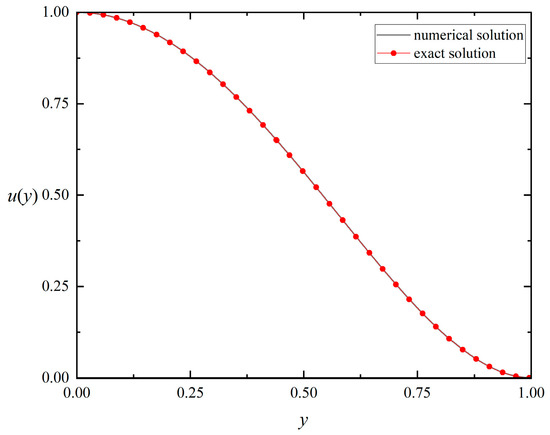
Figure 2. The comparison curve of error distribution for $T=1$ between the numerical solution and the exact solution when $\beta =0.5$, $\eta =1$ and $W=1$.

Figure 3 provides a clear visualization of the disparities in velocity distribution when comparing the ABC against the DTBC, facilitated by the choice of $f(y,t)=0$. Notably, the distribution curves exhibit significant divergence at the right boundary. This difference stems from the fact that the DTBC specifies zero velocity at the selected right boundary, whereas the velocity at the right boundary follows a specific functional relationship when subject to the ABC, which is determined through meticulous derivation. In numerous practical situations, the velocity at the boundary on the right does not maintain a constant zero over time, which potentially results in imprecise numerical solutions based on the DTBC. However, the ABC averts the artificial error at the truncation point and is consistent with the zero boundary condition at infinite locations. This proves that the ABC can effectively deal with problems related to extension to infinite domains.

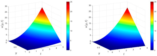
Figure 3. The velocity distribution between the ABC (left) and the DTBC (right) when $f(y,t)=0$, $T=5$, $\beta =0.5$, $\eta =1$, and $W=1$.

5.2. Impact of Parameter Variations on the Velocity Field Induced by a Moving Plate

We assume that the fluid is set in motion by a plate moving at the velocity $u_w(t)=W{t}^2$. With this assumption, the governing equation with its associated IBCs reduces to:

$$\frac{\partial u(y,t)}{\partial t}=\frac{{\partial }^{2}u(y,t)}{\partial y^2}+\eta {}_0{}^{RL}\mathcal{D}_t^{\beta }\frac{{\partial }^{2}u(y,t)}{\partial y^2}$$

(72)

$$u\left(y,0\right)=0 \mathrm{for} y>0$$

(73)

$$u\left(0,t\right)=W{t}^2 \mathrm{and} \frac{\partial u(y_r,t)}{\partial y}+{\displaystyle {\int }_0^t{K}_1(t-\tau )\ast {}_0{}^{RL}\mathcal{D}_{\tau }^{1/2}u}(y_r,\tau )\mathrm{d}\tau =0$$

(74)

The examination of parameter influence on the velocity field is conducted. In this example, we select the cut-off point as $y_r=8$. Figure 4 illustrates the impact of the varying time parameter on the velocity distribution. Comparing multiple curves at different time points, it can be found that the fluid velocity at the same location increases with time. Analyzing a single curve, it can be observed that the closer the fluid is to the plate, the greater the velocity will be. The figure describes the time evolution of the velocity well.

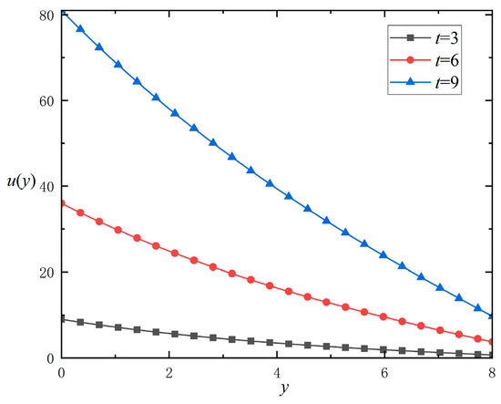
Figure 4. The impacts exerted by the time parameters on the velocity distribution for $\beta =0.5$, $\eta =1$, and $W=1$.

As shown in Figure 5 for $y$ (left) and $t$ (right), the variation in fractional orders significantly influences the velocity distribution. This plate’s motion changes the shear force, causing the fluid near the plate to begin to flow. Therefore, it can be observed that in the actual image, the velocity at the starting point is very high, whereas the velocity at locations further away is relatively low. A trend is observable in these images, where the flow velocity diminishes with an increase in $y$. And at a fixed position, the velocity rises with the augmentation of $t$. As shown in the figure on the left of Figure 5, at a fixed time, the increase in the fractional parameter results in a smaller value of the distribution curve. From this, it can be observed that as the fractional parameter diminishes, the fluid’s memory properties become more pronounced, and the velocity transmission occurs more rapidly. Regarding the relationship between the distribution curve and time, when the spatial position is fixed, the larger fractional parameter results in the decreasing velocity of the fluid.

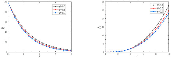
Figure 5. The impacts exerted of the fractional parameters on the velocity distribution versus $y$ ($t=1$) and $t$ ($y=1$) for $\eta =1$ and $W=1$.

In Figure 6, the effect of relaxation parameters on the velocity distribution is shown. The relaxation time parameter exerts a delayed impact on the fluid’s flow. As illustrated on the left side of Figure 6, at a fixed time, an increase in the relaxation parameter results in a higher value of the distribution curve. From this observation, a conclusion can be drawn that there is a correlation between the larger relaxation parameter and the delay effect. For the relationship between the distribution curve and time, when the space y is fixed, the velocity increases as the relaxation parameter becomes larger.

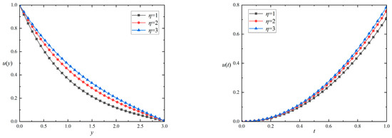
Figure 6. The impacts of the relaxation parameters on the velocity distribution versus $y$ ($t=1$) and $t$ ($y=1$) for $\beta =0.5$ and $W=1$.

Figure 7 demonstrates the distribution versus $\beta$ with the influence of various relaxation time parameters, highlighting the relaxation time parameter’s delayed influence on fluid flow. As depicted in Figure 7, for a constant fractional parameter $\beta$, an increase in the relaxation parameter leads to a higher value of the distribution curve. Concurrently, with the fractional parameter increasing, the fluid velocity diminishes progressively. It is inferred that a larger relaxation parameter results in a diminished delay effect and an increased velocity.

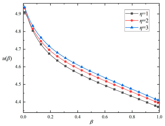
Figure 7. The impacts of the relaxation parameters on the velocity distribution versus $\beta$ for $W=1$.

5.3. Various Velocities Induced by Vibrating Plates with Different Physical Parameters

In this example, the emphasis is placed on the impact of dynamic parameters on the flow mechanism of fluid, propelled by a plate with oscillating velocity. The governing equation for the IBCs is presented below

$$\frac{\partial u(y,t)}{\partial t}=\frac{{\partial }^{2}u(y,t)}{\partial y^2}+\eta {}_0{}^{RL}D_t^{\beta }\frac{{\partial }^{2}u(y,t)}{\partial y^2}$$

(75)

$$u\left(y,0\right)=0 \mathrm{for} y>0$$

(76)

$$u\left(0,t\right)=U\sin \left(\omega t^2\right) \mathrm{and} \frac{\partial u(y_r,t)}{\partial y}+{\displaystyle {\int }_0^t{K}_1(t-\tau )\ast {}_0{}^{RL}\mathcal{D}_{\tau }^{1/2}u}(y_r,\tau )\mathrm{d}\tau =0$$

(77)

Figure 8 shows the velocity distribution of $y$ and $t$. Contrary to previous numerical instances, the observations from the figure reveal that the oscillating distribution results directly from a moving plate exhibiting oscillatory velocity. The effects of frequency $\omega$ and amplitude $U$ on the velocity distribution on $y$ and $t$ are shown in Figure 9 and Figure 10. It should be noted that we took the space calculation region as $\left[0,5\right]$, and the termination time of the analysis was $T=5$.

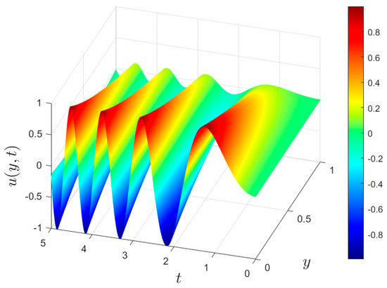
Figure 8. The velocity distributions with $y$ and $t$ for $\beta =0.5$, $\eta =1$, $\omega =1$, and $U=1$.

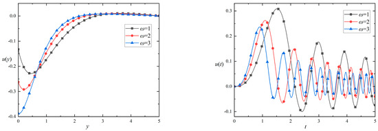
Figure 9. The velocity distributions with different frequency $\omega$ versus $y$ ($t=5$) and $t$ ($y=1$) for $\beta =0.5$, $U=1$, and $\eta =1$.

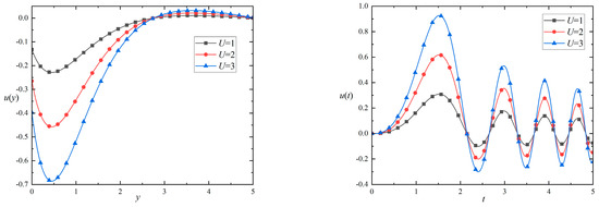
Figure 10. The velocity distributions with different amplitudes $U$ versus $y$ ($t=5$) and $t$ ($y=1$) for $\beta =0.5$, $\omega =1$, and $\eta =1$.

Figure 9 illustrates the impact of the oscillation frequency $\omega$ on the velocity distribution. In the left figure, at a fixed time, the fluid near the moving plate has a larger negative velocity in the initial position. The fluid’s velocity increases with the moving plate’s vibration frequency $\omega$. Due to the vibration of the moving plate, the peak value of the velocity distribution curve occurs within a certain distance from the plate when $\omega =1$ and $\omega =2$, while the curve does not oscillate when $\omega =3$. With the increase in $y$, the influence of oscillations on the fluid weakens and the fluid velocity decreases in the negative direction. By comparing the velocity distribution curves at different frequencies, it can be observed that the velocity distribution curve of the fluid changes more rapidly as the frequency $\omega$ of the moving plate increases. Finally, when the distance from the plate is far enough, the vibration of the plate has no effect on the fluid. The velocity distribution curve of the fluid becomes smoother, and the velocity distribution curves of different vibration frequencies tend to be close. In the figure on the right, the time change of the fluid near the plate, which is affected by the moving plate, is described. For the same vibration frequency $\omega$, the amplitude of the velocity distribution curve and the vibration period gradually decrease with the passage of time, because the moving plate whose velocity oscillates in the form of a sinusoidal function causes the fluctuation of the velocity distribution. The peak value of the velocity distribution curve is earlier for a larger vibration frequency $\omega$. The results show that, as the frequency $\omega$ increases, both the period and the amplitude of the distribution curve decrease.

Figure 10 depicts the impact of the amplitude on the velocity distribution. Similar to Figure 9, the negative velocity of the fluid close to the moving plate first increases to the peak and then decreases. At a fixed position, the oscillation period and amplitude of the fluid decrease gradually with the passage of time. By comparing the velocity distribution curves of different amplitudes, the larger the amplitude $U$ is, the greater the peak value of the velocity distribution curve at a fixed time is, and the faster the curve changes. In a fixed position, the velocity distribution curve’s amplitude is directly proportional to the amplitude $U$.

5.4. Comparison of This Study with Other Methods in Ref. [58]

To further verify the accuracy of the numerical solutions presented in this paper, other studies on generalized second-order fluid flow on a semi-infinite plate are selected for comparison. Shahed [58] studied the impulsive flow of a fractional second-grade fluid on a flat plate. The IBCs were $u(y,0)=0$, $y>0$, $u\left(0,t\right)=1$, $u\left(+\infty ,t\right)=0$, and $t\in \left[0,T\right]$.

Since the initial condition is zero, the equation containing the Caputo fractional derivative in reference [58] is equivalent to the equation with RLTFD in this paper. The ABC (32) is applied. By selecting the same parameters and comparing them with Figure 2 in [58], the comparison curve with the numerical solution in our study is given in Figure 11. The red dotted line is the curve derived from the method of this study, and the black solid line is the curve given by Shahed [58]. The comparison shows that the curves derived from the two methods match very well, which indicates the accuracy of our numerical method.

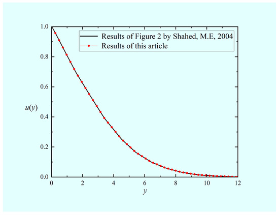
Figure 11. Comparison between the numerical solution in our study and other methods in Ref. [58] by selecting parameters $\eta =1$, $t=2$, and $\beta =0.5$.

6. Conclusions

In this study, the fractional governing equation that describes generalized second-grade fluid’s flow over semi-infinite plates, induced by varying plate velocities, was rigorously derived. For semi-bounded domains, the study employed the ABM. This resulted in the formulation of ABC as convolutions within a finite region. The use of the artificial boundary method made the numerical simulation of this fractional governing equation highly applicable. Subsequently, the governing equation was numerically discretized by incorporating the initial condition and the ABC by utilizing the L1 scheme. The paper then presented four numerical examples: the first one validated the difference scheme’s effectiveness through introducing the source term and demonstrated the superiority of the ABC compared to the DTBC, and the second one examined how dynamic parameters within the governing equation affect velocity distribution. In the third example, a numerical example was given to analyze the flow mechanism arising from an oscillating plate, and the effects of the frequency and amplitude on velocity were described, respectively. Finally, the comparison of the numerical example with the ABC and the results in Ref. [58] was discussed. Some of the major findings are summarized below.

(i)

A higher fractional parameter leads to a slower rate of fluid flow;

(ii)

The delay effect increases with the decrease in relaxation parameters, and the fluid velocity rises as the relaxation parameter increases;

(iii)

The higher the oscillation frequency is, the faster the velocity will change, and the velocity distribution curve will exhibit a decreased period and amplitude;

(iv)

With a greater amplitude, the fluid velocity changes more rapidly and the amplitude of the velocity distribution curve also increases.

The important conclusions drawn from this study not only advance the theory of non-Newtonian fluid dynamics, but also extend to its engineering applications in a broad spectrum of fields, including chemical, petroleum, aerospace, and biomedical engineering. In addition, this research contributes to the design and optimization of new materials in materials science, the prediction of pollutant dispersion in environmental science, and the diagnosis and treatment of cardiovascular diseases in the medical field. It also promotes the advancement of numerical simulation technology to solve the problem of infinite boundaries using artificial boundary techniques and provides a theoretical basis and computational methods for the simulation of complex fluid systems. We intend to explore more comprehensive non-Newtonian fluid models with ABC is our future work.

References

- Mohamed, A.A.; Khishvand, M.; Piri, M. Entrapment and mobilization dynamics during the flow of viscoelastic fluids in natural porous media: A micro-scale experimental investigation. Phys. Fluids 2023, 35, 047119. [Google Scholar] [CrossRef]
- Steinhaus, B.; Shen, A.Q.; Sureshkumar, R. Dynamics of viscoelastic fluid filaments in microfluidic devices. Phys. Fluids 2007, 19, 073103. [Google Scholar] [CrossRef]
- Lauga, E. Propulsion in a viscoelastic fluid. Phys. Fluids 2007, 19, 083104. [Google Scholar] [CrossRef]
- VeeraKrishna, M.; Chamkha, A.J. Hall effects on unsteady MHD flow of second grade fluid through porous medium with ramped wall temperature and ramped surface concentration. Phys. Fluids 2018, 30, 053101. [Google Scholar] [CrossRef]
- Wang, S.; Tai, C.W.; Narsimhan, V. Dynamics of spheroids in an unbound quadratic flow of a general second-grade fluid. Phys. Fluids 2020, 32, 113106. [Google Scholar] [CrossRef]
- Ho, B.P.; Leal, L.G. Migration of rigid spheres in a two-dimensional unidirectional shear flow of a second-grade fluid. J. Fluid Mech. 1976, 76, 783–799. [Google Scholar] [CrossRef]
- Khan, M.; Wang, S. Flow of a generalized second-grade fluid between two side walls perpendicular to a plate with a fractional derivative model. Nonlinear Anal. Real World Appl. 2009, 10, 203–208. [Google Scholar] [CrossRef]
- Tassaddiq, A. MHD flow of a fractional second grade fluid over an inclined heated plate. Chaos Soliton. Fract. 2019, 123, 341–346. [Google Scholar] [CrossRef]
- Metzne, A.B.; Park, M.G. Turbulent flow characteristics of viscoelastic fluids. J. Fluid Mech. 1964, 20, 291–303. [Google Scholar] [CrossRef]
- Li, G.; McKinley, G.H.; Ardekani, A.M. Dynamics of particle migration in channel flow of viscoelastic fluids. J. Fluid Mech. 2015, 785, 486–505. [Google Scholar] [CrossRef]
- Billingham, J.; King, A.C. The interaction of a moving fluid/fluid interface with a flat plate. J. Fluid Mech. 1995, 296, 325–351. [Google Scholar] [CrossRef]
- Traugott, S.C. Impulsive Motion of an Infinite Plate in a Compressible Fluid with Non-Uniform External Flow. J. Fluid Mech. 1962, 13, 400–416. [Google Scholar] [CrossRef]
- Jaworski, J.W.; Peake, N. Aerodynamic noise from a poroelastic edge with implications for the silent flight of owls. J. Fluid Mech. 2013, 723, 456–479. [Google Scholar] [CrossRef]
- Sahoo, T.; Yip, T.L.; Chwang, A.T. Scattering of surface waves by a semi-infinite floating elastic plate. Phys. Fluids 2001, 13, 3215–3222. [Google Scholar] [CrossRef]
- Baranovskii, E.S. Exact solutions for non-isothermal flows of second grade fluid between parallel plates. Nanomaterials 2023, 13, 1409. [Google Scholar] [CrossRef] [PubMed]
- Baranovskii, E.S. Analytical Solutions to the Unsteady Poiseuille Flow of a Second Grade Fluid with Slip Boundary Conditions. Polymers 2024, 16, 179. [Google Scholar] [CrossRef] [PubMed]
- Du, M.; Wang, Z.; Hu, H. Measuring memory with the grade of fractional derivative. Sci. Rep. 2013, 3, 3431. [Google Scholar] [CrossRef] [PubMed]
- Carpinteri, A.; Francesco, M. Fractals and Fractional Calculus in Continuum Mechanics; Springer: Berlin/Heidelberg, Germany, 2014; Volume 378. [Google Scholar]
- Uchaikin, V.; Renat, S. Fractional Kinetics in Space: Anomalous Transport Models; World Scientific: Singapore, 2018. [Google Scholar]
- Tarasov, V.E. Fractional Dynamics: Applications of Fractional Calculus to Dynamics of Particles, Fields and Media; Springer Science & Business Media: Berlin/Heidelberg, Germany, 2011. [Google Scholar]
- Shen, M.; Chen, L.; Zhang, M.; Liu, F. A renovated Buongiorno’s model for unsteady Sisko nanofluid with fractional Cattaneo heat flux. Int. J. Heat Mass Transf. 2018, 126, 277–286. [Google Scholar] [CrossRef]
- Sene, N. Second-grade fluid model with Caputo-Liouville generalized fractional derivative. Chaos Soliton. Fract. 2020, 133, 109631. [Google Scholar] [CrossRef]
- Chan, P.C.H.; Leal, L.G. The motion of a deformable drop in a second-grade fluid. J. Fluid Mech. 1979, 92, 131–170. [Google Scholar] [CrossRef]
- Jiang, X.; Zhang, H.; Wang, S. Unsteady magnetohydrodynamic flow of generalized second grade fluid through porous medium with Hall effects on heat and mass transfer. Phys. Fluids 2020, 32, 113105. [Google Scholar] [CrossRef]
- Deswal, S.C.R.; Kalkal, K.K. Fractional grade heat conduction law in micropolar thermo-viscoelasticity with two temperatures. Int. J. Heat Mass Transf. 2013, 66, 451–460. [Google Scholar] [CrossRef]
- Wang, X.; Xu, H.; Qi, H. Transient magnetohydrodynamic flow and heat transfer of fractional Oldroyd-B fluids in a microchannel with slip boundary condition. Phys. Fluids 2020, 32, 103104. [Google Scholar] [CrossRef]
- Awad, E. Dual-phase-lag in the balance Sufficiency bounds for the class of Jeffreys’ equations to furnish physical solutions. Int. J. Heat Mass Transf. 2020, 158, 119742. [Google Scholar] [CrossRef]
- Coppola, G.; Veldman, A.E.P. Global and local conservation of mass, momentum and kinetic energy in the simulation of compressible flow. J. Comput. Phys. 2023, 475, 111879. [Google Scholar] [CrossRef]
- Tamim, S.; Bostwick, J.B. Spreading of a thin droplet on a soft substrate. J. Fluid Mech. 2023, 971, A32. [Google Scholar] [CrossRef]
- Mei, R.; Adrian, R.J. Flow past a sphere with an oscillation in the free-stream velocity and unsteady drag at finite Reynolds number. J. Fluid Mech. 1992, 237, 323–341. [Google Scholar] [CrossRef]
- Dennis, S.C.R. Calculation of the steady flow through a curved tube using a new finite-difference method. J. Fluid Mech. 1980, 99, 449–467. [Google Scholar] [CrossRef]
- Kim, T.Y.; Dolbow, J.; Fried, E. A numerical method for a second-gradient theory of incompressible fluid flow. J. Comput. Phys. 2007, 223, 551–570. [Google Scholar] [CrossRef]
- Gilmanov, A.; Sotiropoulos, F. A hybrid Cartesian/immersed boundary method for simulating flows with 3D, geometrically complex, moving bodies. J. Comput. Phys. 2005, 207, 457–492. [Google Scholar] [CrossRef]
- Li, B.; Zhang, J.; Zheng, C. Stability and error analysis for a second-grade fast approximation of the one-dimensional Schrödinger equation under absorbing boundary conditions. SIAM J. Sci. Comput. 2018, 40, A4083–A4104. [Google Scholar] [CrossRef]
- Uhlmann, M. An immersed boundary method with direct forcing for the simulation of particulate flows. J. Comput. Phys. 2005, 209, 448–476. [Google Scholar] [CrossRef]
- Özdemir, N.; Karadeniz, D.; İskender, B.B. Fractional optimal control problem of a distributed system in cylindrical coordinates. Phys. Lett. A 2009, 373, 221–226. [Google Scholar] [CrossRef]
- Yan, Y.; Khan, M.; Ford, N.J. An analysis of the modified L1 scheme for time-fractional partial differential equations with nonsmooth data. SIAM J. Numer. Anal. 2018, 56, 210–227. [Google Scholar] [CrossRef]
- Lyu, P.; Vong, S. A nonuniform L2 formula of Caputo derivative and its application to a fractional Benjamin-Bona-Mahony-type equation with nonsmooth solutions. Numer. Meth. Part Differ. Equ. 2020, 36, 579–600. [Google Scholar] [CrossRef]
- Xing, Z.; Wen, L. Numerical Analysis of the Nonuniform Fast L1 Formula for Nonlinear Time-Space Fractional Parabolic Equations. J. Sci. Comput. 2023, 95, 58. [Google Scholar] [CrossRef]
- Chen, Z.; Zheng, W. Convergence of the uniaxial perfectly matched layer method for time-harmonic scattering problems in two-layered media. SIAM J. Numer. Anal. 2010, 48, 2158–2185. [Google Scholar] [CrossRef]
- Barucq, H.; Rouxelin, N.; Tordeux, S. Low-grade Prandtl-Glauert-Lorentz based Absorbing Boundary Conditions for solving the convected Helmholtz equation with Discontinuous Galerkin methods. J. Comput. Phys. 2022, 468, 111450. [Google Scholar] [CrossRef]
- Li, B.; Zhang, J.; Zheng, C. An efficient second-grade finite difference method for the one-dimensional Schrödinger equation with absorbing boundary conditions. SIAM J. Numer. Anal. 2018, 56, 766–791. [Google Scholar] [CrossRef]
- Muhr, M.; Nikolić, V.; Wohlmuth, B. Self-adaptive absorbing boundary conditions for quasilinear acoustic wave propagation. J. Comput. Phys. 2019, 388, 279–299. [Google Scholar] [CrossRef]
- Fu, W.; Wang, W.; Li, C.; Huang, S. An investigation of natural convection in parallel square plates with a heated bottom surface by an absorbing boundary condition. Int. J. Heat Mass Transf. 2013, 56, 35–44. [Google Scholar] [CrossRef]
- Baffet, D.; Grote, M.J. On wave splitting, source separation and echo removal with absorbing boundary conditions. J. Comput. Phys. 2019, 387, 589–596. [Google Scholar] [CrossRef]
- Hwang, J.; Jang, J.; Jung, J. The Fokker-Planck equation with absorbing boundary conditions in bounded domains. SIAM J. Math. Anal. 2018, 50, 2194–2232. [Google Scholar] [CrossRef]
- Tan, W.; Masuoka, T. Stokes’ first problem for a second grade fluid in a porous half-space with heated boundary. Int. J. Non-Linear Mech. 2005, 40, 515–522. [Google Scholar] [CrossRef]
- Rivlin, R.S.; Ericksen, J.L.V. Stress-Deformation Relations for Isotropic Materials; Collected Papers of RS Rivlin Volume I and II; Springer: Berlin/Heidelberg, Germany, 1997; pp. 911–1013. [Google Scholar]
- Tan, W.; Xu, M. The impulsive motion of flat plate in a generalized second grade fluid. Mech. Res. Commun. 2002, 29, 3–9. [Google Scholar] [CrossRef]
- Khan, M.; Nadeem, S.; Hayat, T.; Siddiqui, A.M. Unsteady motions of a generalized second-grade fluid. Math. Comput. 2005, 41, 629–637. [Google Scholar] [CrossRef]
- Hilfer, R. Applications of Fractional Calculus in Physics; World Scientific: Singapore, 2000. [Google Scholar]
- Hristov, J. Linear viscoelastic responses and constitutive equations in terms of fractional operators with non-singular kernels-pragmatic approach, memory kernel correspondence requirement and analyses. Eur. Phys. J. Plus 2019, 134, 283. [Google Scholar] [CrossRef]
- Li, C.; Qian, D.; Chen, Y. On Riemann-Liouville and Caputo derivatives. Discrete. Dyn. Nat. Soc. 2011, 2011, 562494. [Google Scholar] [CrossRef]
- Mahmood, A.; Fetecau, C.; Khan, N.A.; Jamil, M. Some exact solutions of the oscillatory motion of a generalized second grade fluid in an annular region of two cylinders. Acta Mech. Sin. 2010, 26, 541–550. [Google Scholar] [CrossRef]
- Podlubny, I. Fractional Differential Equation; Academic Press: San Diego, LA, USA, 1999. [Google Scholar]
- Alikhanov, A.A. A priori estimates for solutions of boundary value problems for fractional-grade equations. Differ. Equ. 2010, 46, 660–666. [Google Scholar] [CrossRef]
- Feng, L.; Liu, F.; Turner, I.; Zheng, L. Novel numerical analysis of multi-term time fractional viscoelastic non-Newtonian fluid models for simulating unsteady MHD Couette flow of a generalized Oldroyd-B fluid. Fract. Calc Appl. Anal. 2018, 21, 1073–1103. [Google Scholar] [CrossRef]
- Shahed, M.E. On the impulsive motion of flat plate in a generalized second grade fluid. Z. Naturfors. Sect. A-J. Phys. Sci. 2004, 59, 829–837. [Google Scholar]
Disclaimer/Publisher’s Note: The statements, opinions and data contained in all publications are solely those of the individual author(s) and contributor(s) and not of MDPI and/or the editor(s). MDPI and/or the editor(s) disclaim responsibility for any injury to people or property resulting from any ideas, methods, instructions or products referred to in the content. |
© 2024 by the authors. Licensee MDPI, Basel, Switzerland. This article is an open access article distributed under the terms and conditions of the Creative Commons Attribution (CC BY) license (https://creativecommons.org/licenses/by/4.0/).