Article

Fractional-Order Dynamics in Epidemic Disease Modeling with Advanced Perspectives of Fractional Calculus

1
Department of Mathematics, University of Malakand, Chakdara 18000, Khyber Pakhtunkhwa, Pakistan
2
Department of Mathematical Sciences, College of Science, Princess Nourah bint Abdulrahman University, P.O. Box 84428, Riyadh 11671, Saudi Arabia
3
EIAS Data Science and BlockChain Laboratory, College of Computer and Information Sciences, Prince Sultan University, Riyadh 11586, Saudi Arabia
4
Department of Electronics and Communications Engineering, Zagazig University, Zagazig 44519, Egypt
*
Author to whom correspondence should be addressed.
Fractal Fract. 2024, 8(5), 291; https://doi.org/10.3390/fractalfract8050291
Submission received: 1 April 2024 / Revised: 3 May 2024 / Accepted: 10 May 2024 / Published: 15 May 2024

Abstract

:
Piecewise fractional-order differential operators have received more attention in recent years because they can be used to describe various evolutionary dynamical problems to investigate crossover behaviors. In this manuscript, we use the aforementioned operators to investigate a mathematical model of COVID-19. By utilizing fractional calculus, our approach aims to capture the crossover dynamics of disease spread, considering heterogeneity and transitions between epidemic phases. This research seeks to develop a framework using specialized mathematical techniques, such as the Caputo fractional derivative, with the potential to investigate the crossover dynamical behaviors of the considered epidemic model. The anticipated contribution lies in bridging fractional calculus and epidemiology, offering insights for both theoretical advancements and practical public health interventions. In order to improve our understanding of epidemic dynamics and support, we used MATLAB to simulate numerical results for a visual representation of our findings. For this interpretation, we used various fractional-order values. In addition, we also compare our simulated results with some reported results for infected and death classes to demonstrate the efficiency of our numerical method.

1. Introduction

Infectious diseases continue impacting a vast global population, despite ongoing advancements in treatment and prevention. Efficient control necessitates the precise management of factors such as transmissibility, population size, contact rates, and infection duration. One of the most important aspects of understanding and managing illness processes is mathematical modeling, particularly when vaccination is inaccessible or during the early stages of a disease. Recently, the study of biological models of infectious diseases has experienced a notable surge in popularity. Numerous mathematical models in the literature capture the dynamics of various infectious diseases. These models, like SIR models, often use three populations at time t : recovered people R, infectious I, and susceptible S. Key contributions in the early twentieth century by Ross [1], Ross and Hudson [2], and Kermack and Mc Kendricks [3] established the groundwork for these models. An additional compartment, called the exposed class E has been included for individuals who have been incubated but are not yet infectious in the infection phase. The studies in [4,5] investigated disease transmission rates using saturated, bilinear, and fractional incidence rates. Many diseases, such as human immunodeficiency virus [6], tuberculosis [7], influenza [8], and dengue fever [9], exhibit a variation process, potentially leading to the emergence of multiple pathogen strains. Therefore, a multi-strain model is more effective in describing diseases caused by multiple epidemic strains. Previous research on the SEIR multi-strain model assumed homogenous mixtures for all strains [10,11].
In recent times, there has been a notable surge in the exploration of definitions and fractional derivatives. Pure mathematicians aim to expand current definitions by generalizing beyond basic power functions, incorporating a broader range of kernel functions. This work was motivated by the need to confront the intrinsic complexity of fractional calculus, which was previously disregarded in engineering since it appeared to be self-contained in integer-order calculus and had no obvious geometrical or physical meaning. While fractional calculus has ancient roots, it has only recently gained traction in mathematical applications. The growing curiosity of humans has led to the development of new ideas, aiding in better understanding complex challenges encountered daily. Real-world applications of fractional differential calculus principles have become apparent, especially in situations where traditional derivatives, whether fractional- or integer-order, fall short in describing rapid changes seen in phenomena like earthquakes, weather dynamics, economic fluctuations in developing countries, and even events within the human body.
To address these challenges, a different type of derivative known as piecewise is required to adequately represent phenomena characterized by crossover behavior. Differential equations incorporating such piecewise derivatives find wide-ranging applications in modeling evolution problems. The authors of [12] introduced various operators to tackle real-world problems, offering a novel approach that effectively represents evolution phenomena experiencing crossover behavior. Fractional calculus is used in many areas, including chemistry, probability, diffusion, rheology, transport theory, and quantitative biology [13]. A recent study investigated bilinear and non-monotonic types of incidence for infection growth in a population using a mathematical model with two strains and two infected classes [14]. In [15], this model was examined in further detail using two non-monotonic incidence rates. Subsequently, ref. [16] expanded these models by incorporating exposed individuals for each strain. The authors of [17] studied a two-strain model for the mentioned infectious diseases.
To explore the concept of fractional calculus in epidemic modeling, we refer to [18,19,20,21]. For the recent advances in fractional-order mathematical models with a piecewise fractional differential operator, we refer to [22,23,24,25,26].
In extending the idea of derivatives to non-integer orders, fractional calculus provides a strong mathematical foundation that makes it possible to characterize intricate and unusual behaviors in dynamical systems. In particular, a piecewise fractional differential operator provides a more effective approach to investigating epidemic models compared to ordinary differential operator because of numerous important benefits. These operators can more precisely describe the complex dynamics seen in epidemics, such as population heterogeneity and non-linear interactions.
Motivated by the aforementioned information, we present our approach to investigate the fractional dynamics of an existing modified model (1) studied in [27], which is represented by a set of ordinary differential equations (ODEs), using the advanced perspective of fractional calculus. The authors studied the dynamics of the aforementioned COVID-19 model using Volterra–Lyapunov matrix theory. Our goal was to extend the traditional framework by incorporating fractional derivatives and exploring its advanced techniques to enhance our understanding of the system’s behavior beyond the limitations of integer-order models.
d S ( t ) d t = σ β 1 1 + η I ( t ) I ( t ) + μ + γ S ( t ) , d E ( t ) d t = γ S ( t ) + α C ( t ) β 2 ρ I ( t ) + μ + τ E ( t ) , d C ( t ) d t = τ E ( t ) [ α + μ ] C ( t ) , d I ( t ) d t = β 1 S ( t ) 1 + η I ( t ) + β 2 ρ E ( t ) μ δ ϵ I ( t ) , d Q ( t ) d t = δ I ( t ) [ μ + k + λ ] Q ( t ) , d D ( t ) d t = ϵ I ( t ) + k Q ( t ) , d R ( t ) d t = λ Q ( t ) μ R ( t ) .
With the help of the aforementioned theory, the authors established a detailed analysis for global, and local stability. In addition, the authors used a nonstandard finite difference method for the numerical simulations.
To extend the traditional framework by incorporating the advanced perspective of fractional calculus, we used a piecewise fractional differential operator to investigate the epidemic model (1). The model is formulated in terms of a piecewise derivative as follows:
D t ϑ 0               PWC [ S ( t ) ] = σ β 1 1 + η I ( t ) I ( t ) + μ + γ S ( t ) , D t ϑ 0               PWC [ E ( t ) ] = γ S ( t ) + α C ( t ) β 2 ρ I ( t ) + μ + τ E ( t ) , D t ϑ 0               PWC [ C ( t ) ] = τ E ( t ) [ α + μ ] C ( t ) , D t ϑ 0               PWC [ I ( t ) ] = β 1 S ( t ) 1 + η I ( t ) + β 2 ρ E ( t ) μ δ ϵ I ( t ) , D t ϑ 0               PWC [ Q ( t ) ] = δ I ( t ) [ μ + k + λ ] Q ( t ) , D t ϑ 0               PWC [ D ( t ) ] = ϵ I ( t ) + k Q ( t ) , D t ϑ 0               PWC [ R ( t ) ] = λ Q ( t ) μ R ( t ) .
Here, the notation D t ϑ 0               PWC is used for the piecewise fractional-order derivative with order ϑ ( 0 , 1 ] . Table 1 describes the compartments and nomenclature of model (2).
We show a diagram of our suggested model in Figure 1.
We present some details about the basic reproductive number and equilibrium points. A detailed analysis for the existence theory was established using the procedure presented in [28]. In addition, we deduced the numerical algorithm based on interpolation technique, for which its details can be found in [29]. Various graphical representations are presented using different fractional-order values.
Organization of the paper: Section 2 provides a thorough overview of the core concepts required to understand the subsequent studies. Section 3 focuses on the key findings and analysis of our study. Section 4 focuses on the technical aspects of our methodology, with a particular focus on the numerical technique employed in the simulations. In Section 5, we present the simulation of the numerical results graphically. Section 6 is devoted to the discussion and comparison of numerical results. Finally, a brief conclusion of the major findings, drawn from our research, is provided in Section 7.

2. Preliminaries

This section highlights the crucial and pertinent themes addressed in the article. We consider V = [ 0 , T ] , V 1 = [ 0 , t 1 ] , and V 2 = ( t 1 , T ] .
Definition 1 
([12]). The definition of the integral operator for a differentiable function z is given for both classical and fractional orders as follows:
I t ϑ 0           PW ( t ) = 0 t 1 z ( θ ) d θ , t V 1 , 1 Γ ( ϑ ) t 1 t ( t θ ) ϑ 1 z ( θ ) d ( θ ) , t V 2 ,
where I t 0           PW denotes two integrals: a classical one for t V 1 , and a Riemann–Liouville integral for t V 2 .
Definition 2 
([12]). Let z C ( V ) be a differentiable function. Then, we define the required operator as follows:
D t ϑ 0               PWC z ( t ) = z ( t ) , t V 1 , D t ϑ 0 C z , t V 2 .
Lemma 1 
([12]). For solving piecewise fractional-order differential equations,
D t ϑ 0               PWC z ( t ) = G ( t , z ( t ) ) , 0 < ϑ 1 ,
is defined as
z ( t ) = 0 t G ( θ , z ( θ ) ) d θ + z 0 , t V 1 , z ( t 1 ) + 1 Γ ( ϑ ) t 1 t ( t θ ) ϑ 1 G ( θ , z ( θ ) ) d ( θ ) , t V 2 .

3. Main Results and Analysis

The quantity denoted by R 0 and the equilibrium points of model (24), including both disease-free equilibrium (DFE) and endemic equilibrium (EE), can be deduced using the procedure described here [17,30]. When R 0 < 1 , it signifies stability at the DFE, suggesting that the disease agent will fade out. Conversely, if R 0 > 1 , the disease is expected to endure. Below, the basic reproduction number R 0 for model (24) is presented, as in [27]:
R 0 = σ μ ( μ + γ ) ( μ + α + τ ) ( μ + δ + ϵ ) β 1 ( μ + α + τ ) μ + β 2 ( μ + α ) ρ γ .
The 3D profile of R 0 is presented in Figure 2 using the numerical values provided in Table 2 for the parameters of (3).
The DFE and an EE points, E 0 and E * , respectively, are stated as follows: E 0 = σ μ + γ , 0 , 0 , 0 , 0 , 0 , 0 , and E * follows from the particular values of S * , E * , C * , Q * , D * , and R * in term of I * as given below:
S * = σ ( 1 + η I * ) ( μ + γ ) + ( β 1 + I * ( μ + γ ) η ) , E * = I * ( μ + σ + ϵ ) ( β 1 I * + ( μ + γ ) ( 1 + η I * ) ) β 1 σ I * β 2 I * ρ , C * = τ ( I * ( μ + σ + ϵ ) ( β 1 I * + ( μ + γ ) ( 1 + η I * ) ) β 1 σ I * ) β 2 ρ ( α + μ ) I * , Q * = 1 ( μ + k + λ ) δ I * , D * = ϵ I * k , R * = λ δ I * ( μ 2 + μ ( k + λ ) ) .

Existence Theory

In this section, we define the Banach space for our investigation. Consider X = J × R 7 R , where J = [ 0 , τ ] , for 0 < t < τ < , with a norm defined by
( S , E , C , I , Q , D , R ) = max t J | S | + | E | + | C | + | I | + | Q | + | D | + | R | .
Then, clearly, ( X , . ) is a Banach space. Now, in considering system (24) in the piecewise fractional derivative,
D t ϑ 0               PWC ( S ( t ) ) = d S d t = σ β 1 1 + η I ( t ) I ( t ) + μ + γ S ( t ) = Ψ 1 ( t , S ( t ) ) , t V 1 , D t ϑ 0 C S = σ β 1 1 + η I ( t ) I ( t ) + μ + γ S ( t ) = Ψ 1 ( t , S ( t ) ) , t V 2 , D t ϑ 0               PWC ( E ( t ) ) = d E d t = γ S ( t ) + α C ( t ) β 2 ρ I ( t ) + μ + τ E ( t ) = Ψ 2 ( t , E ( t ) ) , t V 1 , D t ϑ 0 C E = γ S ( t ) + α C ( t ) β 2 ρ I ( t ) + μ + τ E ( t ) = Ψ 2 ( t , E ( t ) ) , t V 2 , D t ϑ 0               PWC ( C ( t ) ) = d C d t = τ E ( t ) [ α + μ ] C ( t ) = Ψ 3 ( t , C ( t ) ) , t V 1 , D t ϑ 0 C C = τ E ( t ) [ α + μ ] C ( t ) = Ψ 3 ( t , C ( t ) ) , t V 2 , D t ϑ 0               PWC ( I ( t ) ) = d I d t = β 1 S ( t ) 1 + η I ( t ) + β 2 ρ E ( t ) μ δ ϵ I ( t ) = Ψ 4 ( t , I ( t ) ) , t V 1 , D t ϑ 0 C I = β 1 S ( t ) 1 + η I ( t ) + β 2 ρ E ( t ) μ δ ϵ I ( t ) = Ψ 4 ( t , I ( t ) ) , t V 2 , D t ϑ 0               PWC ( Q ( t ) ) = d Q d t = δ I ( t ) [ μ + k + λ ] Q ( t ) = Ψ 5 ( t , Q ( t ) ) , t V 1 , D t ϑ 0 C Q = δ I ( t ) [ μ + k + λ ] Q ( t ) = Ψ 5 ( t , Q ( t ) ) , t V 2 , D t ϑ 0               PWC ( D ( t ) ) = d D d t = ϵ I + k Q = Ψ 6 ( t , D ( t ) ) , t V 1 , D t ϑ 0 C D = ϵ I + k Q = Ψ 6 ( t , D ( t ) ) , t V 2 , D t ϑ 0               PWC ( R ( t ) ) = d R d t = λ Q μ R = Ψ 7 ( t , R ( t ) ) , t V 1 , D t ϑ 0 C R = λ Q μ R = Ψ 7 ( t , R ( t ) ) , t V 2 .
Theorem 1. 
The solution of (4) is given by
S ( t ) = S 0 + 0 t Ψ 1 ( θ , S ( θ ) ) d θ , t V 1 , S ( t 1 ) + 1 Γ ( ϑ ) t 1 t ( t θ ) ϑ 1 Ψ 1 ( θ , S ( θ ) ) d θ , t V 2 , E ( t ) = E 0 + 0 t Ψ 2 ( θ , E ( θ ) ) d θ , t V 1 , E ( t 1 ) + 1 Γ ( ϑ ) t 1 t ( t θ ) ϑ 1 Ψ 2 ( θ , E ( θ ) ) d θ , t V 2 , C ( t ) = C 0 + 0 t Ψ 3 ( θ , C ( θ ) ) d θ , t V 1 , C ( t 1 ) + 1 Γ ( ϑ ) t 1 t ( t θ ) ϑ 1 Ψ 3 ( θ , C ( θ ) ) d θ , t V 2 , I ( t ) = I 0 + 0 t Ψ 4 ( θ , I ( θ ) ) d θ , t V 1 , I ( t 1 ) + 1 Γ ( ϑ ) t 1 t ( t θ ) ϑ 1 Ψ 4 ( θ , I ( θ ) ) d θ , t V 2 , Q ( t ) = Q 0 + 0 t Ψ 5 ( θ , Q ( θ ) ) d θ , t V 1 , Q ( t 1 ) + 1 Γ ( ϑ ) t 1 t ( t θ ) ϑ 1 Ψ 5 ( θ , Q ( θ ) ) d θ , t V 2 , D ( t ) = D 0 + 0 t Ψ 6 ( θ , D ( θ ) ) d θ , t V 1 , D ( t 1 ) + 1 Γ ( ϑ ) t 1 t ( t θ ) ϑ 1 Ψ 6 ( θ , D ( θ ) ) d θ , t V 2 , R ( t ) = R 0 + 0 t Ψ 7 ( θ , R ( θ ) ) d θ , t V 1 , R ( t 1 ) + 1 Γ ( ϑ ) t 1 t ( t θ ) ϑ 1 Ψ 7 ( θ , R ( θ ) ) d θ , t V 2 .
Proof. 
Lemma 1 makes it simple to acquire the equivalent form (6). □
We now outline a few assumptions in light of (4) as follows:
Hypothesis 1 (H1). 
For fixed real values K Ψ i > 0 , i = 1 , 2 , . . . , 7 at z , z ^ X ,
| Ψ i ( t , z ) Ψ i ( t , z ^ ) | K Ψ i [ | z z ^ | .
Hypothesis 2 (H2). 
For fixed real values c Ψ i , d Ψ i > 0 , i = 1 , 2 , . . . , 7 , one has
| Ψ i ( t , z ^ ) | c Ψ i + d Ψ i | z ^ | .
Here, we define the operator
= ( 1 , 2 , 3 , 4 , 5 , 6 , 7 ) : X X
using Theorem 1 as follows:
1 ( S ) = S 0 + 0 t Ψ 1 ( θ , S ( θ ) ) d θ , t V 1 , S ( t 1 ) + 1 Γ ( ϑ ) t 1 t ( t θ ) ϑ 1 Ψ 1 ( θ , S ( θ ) ) d θ , t V 2 , 2 ( E ) = E 0 + 0 t Ψ 2 ( θ , E ( θ ) ) d θ , t V 1 , E ( t 1 ) + 1 Γ ( ϑ ) t 1 t ( t θ ) ϑ 1 Ψ 2 ( θ , E ( θ ) ) d θ , t V 2 , 3 ( C ) = C 0 + 0 t Ψ 3 ( θ , C ( θ ) ) d θ , t V 1 , C ( t 1 ) + 1 Γ ( ϑ ) t 1 t ( t θ ) ϑ 1 Ψ 3 ( θ , C ( θ ) ) d θ , t V 2 , 4 ( I ) = I 0 + 0 t Ψ 4 ( θ , I ( θ ) ) d θ , t V 1 , I ( t 1 ) + 1 Γ ( ϑ ) t 1 t ( t θ ) ϑ 1 Ψ 4 ( θ , I ( θ ) ) d θ , t V 2 , 5 ( Q ) = Q 0 + 0 t Ψ 5 ( θ , Q ( θ ) ) d θ , t V 1 , Q ( t 1 ) + 1 Γ ( ϑ ) t 1 t ( t θ ) ϑ 1 Ψ 5 ( θ , Q ( θ ) ) d θ , t V 2 , 6 ( D ) = D 0 + 0 t Ψ 6 ( θ , D ( θ ) ) d θ , t V 1 , D ( t 1 ) + 1 Γ ( ϑ ) t 1 t ( t θ ) ϑ 1 Ψ 6 ( θ , D ( θ ) ) d θ , t V 2 , 7 ( R ) = R 0 + 0 t Ψ 7 ( θ , R ( θ ) ) d θ , t V 1 , R ( t 1 ) + 1 Γ ( ϑ ) t 1 t ( t θ ) ϑ 1 Ψ 7 ( θ , R ( θ ) ) d θ , t V 2 .
Here, we define some quantities using max t [ 0 , T ] | S ( t ) | S 0 , max t [ 0 , T ] | E ( t ) | = E ˜ , and max t [ 0 , T ] | I ( t ) | = I ˜ :
K Ψ 1 = β 1 I ˜ + μ + γ , K Ψ 2 = β 2 ρ I ˜ + μ + τ , K Ψ 3 = α + μ , K Ψ 4 = β 1 S 0 + β 2 ρ E ˜ + μ + δ + ϵ , K Ψ 5 = μ + κ + λ , K Ψ 6 = 0 , K Ψ 7 = μ .
Theorem 2. 
In utilizing Hypothesis 1 (H1), the coupled system (4) has a unique solution, provided that the following conditions are satisfied:
max t 1 K Ψ i , ( T t 1 ) ϑ Γ ( ϑ + 1 ) K Ψ i = Ω Ψ i , t 1 , T < 1 ,
where
max K Ψ 1 , K Ψ 2 , K Ψ 3 , K Ψ 4 , K Ψ 5 , K Ψ 6 , K Ψ 7 = K Ψ i .
Proof. 
Using (6), one has
1 ( S ) 1 ( S ^ ) K Ψ 1 t 1 S S ^ , t V 1 , K Ψ 1 ( T t 1 ) ϑ Γ ( ϑ + 1 ) S S ^ , t V 2 ,
2 ( E ) 2 ( E ^ ) K Ψ 2 t 1 E E ^ 1 , t V 1 , K Ψ 2 ( T t 1 ) ϑ Γ ( ϑ + 1 ) E E ^ , t V 2 ,
3 ( C ) 3 ( C ^ ) K Ψ 3 t 1 C C ^ , t V 1 , K Ψ 3 ( T t 1 ) ϑ Γ ( ϑ + 1 ) C C ^ , t V 2 ,
4 ( I ) 4 ( I ^ ) K Ψ 4 t 1 I I ^ , t V 1 , K Ψ 4 ( T t 1 ) ϑ Γ ( ϑ + 1 ) I I ^ , t V 2 ,
5 ( Q ) 5 ( Q ^ ) K Ψ 5 t 1 Q Q ^ , t V 1 , K Ψ 5 ( T t 1 ) ϑ Γ ( ϑ + 1 ) Q Q ^ , t V 2 ,
6 ( D ) 6 ( D ^ ) K Ψ 6 t 1 D D ^ , t V 1 , K Ψ 6 ( T t 1 ) ϑ Γ ( ϑ + 1 ) D D ^ , t V 2 ,
7 ( R ) 7 ( R ^ ) K Ψ 7 t 1 R R ^ , t V 1 , K Ψ 7 ( T t 1 ) ϑ Γ ( ϑ + 1 ) R R ^ , t V 2 .
Now, adding (8)–(14), we obtain
( S , E , C , I , Q , D , R ) ( S ^ , E ^ , C ^ , I ^ , Q ^ , D ^ , R ^ ) t 1 K Ψ i ( S , E , C , I , Q , D , R ) ( S ^ , E ^ , C ^ , I ^ , Q ^ , D ^ , R ^ ) , t V 1 , ( T t 1 ) ϑ Γ ( ϑ + 1 ) K Ψ i ( S , E , C , I , Q , D , R ) ( S ^ , E ^ , C ^ , I ^ , Q ^ , D ^ , R ^ ) , t V 2 .
Again, from (16), we have
( S , E , C , I , Q , D , R ) ( S ^ , E ^ , C ^ , I ^ , Q ^ , D ^ , R ^ ) Ω Ψ i , t 1 , T ( S , E , C , I , Q , D , R ) ( S ^ , E ^ , C ^ , I ^ , Q ^ , D ^ , R ^ ) .
Therefore, the system under consideration has a unique solution. □
Theorem 3. 
In utilizing Hypothesis 2 (H2), the suggested coupled system (4) possesses at least one solution within a bounded, closed, and convex subset:
U m = ( S , E , C , I , Q , D , R ) X : ( S , E , C , I , Q , D , R ) m , where a m > 0 .
Proof. 
Let us define an operator
F = ( F 1 , F 2 , F 3 , F 4 , F 5 , F 6 , F 7 ) : U m U m
by
F 1 ( S ) = S 0 + 0 t Ψ 1 ( θ , S ( θ ) ) d θ , t V 1 , S ( t 1 ) + 1 Γ ( ϑ ) t 1 t ( t θ ) ϑ 1 Ψ 1 ( θ , S ( θ ) ) d θ , t V 2 , F 2 ( E ) = E 0 + 0 t Ψ 2 ( θ , E ( θ ) ) d θ , t V 1 , E ( t 1 ) + 1 Γ ( ϑ ) t 1 t ( t θ ) ϑ 1 Ψ 2 ( θ , E ( θ ) ) d θ , t V 2 , F 3 ( C ) = C 0 + 0 t Ψ 3 ( θ , C ( θ ) ) d θ , t V 1 , C ( t 1 ) + 1 Γ ( ϑ ) t 1 t ( t θ ) ϑ 1 Ψ 3 ( θ , C ( θ ) ) d θ , t V 2 , F 4 ( I ) = I 0 + 0 t Ψ 4 ( θ , I ( θ ) ) d θ , t V 1 , I ( t 1 ) + 1 Γ ( ϑ ) t 1 t ( t θ ) ϑ 1 Ψ 4 ( θ , I ( θ ) ) d θ , t V 2 , F 5 ( Q ) = Q 0 + 0 t Ψ 5 ( θ , Q ( θ ) ) d θ , t V 1 , Q ( t 1 ) + 1 Γ ( ϑ ) t 1 t ( t θ ) ϑ 1 Ψ 5 ( θ , Q ( θ ) ) d θ , t V 2 , F 6 ( D ) = D 0 + 0 t Ψ 6 ( θ , D ( θ ) ) d θ , t V 1 , D ( t 1 ) + 1 Γ ( ϑ ) t 1 t ( t θ ) ϑ 1 Ψ 6 ( θ , D ( θ ) ) d θ , t V 2 , F 7 ( R ) = R 0 + 0 t Ψ 7 ( θ , R ( θ ) ) d θ , t V 1 , R ( t 1 ) + 1 Γ ( ϑ ) t 1 t ( t θ ) ϑ 1 Ψ 7 ( θ , R ( θ ) ) d θ , t V 2 .
Then, from (17), we have
F 1 ( S ) = S 0 + 0 t Ψ 1 ( θ , S ( θ ) ) d θ , t V 1 , S ( t 1 ) + 1 Γ ( ϑ ) t 1 t ( t θ ) ϑ 1 Ψ 1 ( θ , S ( θ ) ) d θ , t V 2 , F 2 ( E ) = E 0 + 0 t Ψ 2 ( θ , E ( θ ) ) d θ , t V 1 , E ( t 1 ) + 1 Γ ( ϑ ) t 1 t ( t θ ) ϑ 1 Ψ 2 ( θ , E ( θ ) ) d θ , t V 2 , F 3 ( C ) = C 0 + 0 t Ψ 3 ( θ , C ( θ ) ) d θ , t V 1 , C ( t 1 ) + 1 Γ ( ϑ ) t 1 t ( t θ ) ϑ 1 Ψ 3 ( θ , C ( θ ) ) d θ , t V 2 , F 4 ( I ) = I 0 + 0 t Ψ 4 ( θ , I ( θ ) ) d θ , t V 1 , I ( t 1 ) + 1 Γ ( ϑ ) t 1 t ( t θ ) ϑ 1 Ψ 4 ( θ , C ( θ ) , I ( θ ) ) d θ , t V 2 , F 5 ( Q ) = Q 0 + 0 t Ψ 5 ( θ , Q ( θ ) ) d θ , t V 1 , Q ( t 1 ) + 1 Γ ( ϑ ) t 1 t ( t θ ) ϑ 1 Ψ 5 ( θ , Q ( θ ) ) d θ , t V 2 , F 6 ( D ) = D 0 + 0 t Ψ 6 ( θ , D ( θ ) ) d θ , t V 1 , D ( t 1 ) + 1 Γ ( ϑ ) t 1 t ( t θ ) ϑ 1 Ψ 6 ( θ , D ( θ ) ) d θ , t V 2 , F 7 ( R ) = R 0 + 0 t Ψ 7 ( θ , R ( θ ) ) d θ , t V 1 , R ( t 1 ) + 1 Γ ( ϑ ) t 1 t ( t θ ) ϑ 1 Ψ 7 ( θ , R ( θ ) ) d θ , t V 2 .
By simplifying and employing Hypothesis 2 (H2), we derive from (18) as follows:
F 1 ( S ) | S 0 | + t 1 c Ψ 1 + d Ψ 1 S | S 0 | + t 1 c Ψ 1 + d Ψ 1 m , t V 1 , | S ( t 1 ) | + ( T t 1 ) ϑ Γ ( ϑ + 1 ) c Ψ 1 + d Ψ 1 S | S ( t 1 ) | + ( T t 1 ) ϑ Γ ( ϑ + 1 ) c Ψ 1 + d Ψ 1 m , t V 2 , F 2 ( E ) | E 0 | + t 1 c Ψ 2 + d Ψ 2 E | E 0 | + t 1 c Ψ 2 + d Ψ 2 m , t V 1 , | E ( t 1 ) | + ( T t 1 ) ϑ Γ ( ϑ + 1 ) c Ψ 2 + d Ψ 2 E | E ( t 1 ) | + ( T t 1 ) ϑ Γ ( ϑ + 1 ) c Ψ 2 + d Ψ 2 m , t V 2 , F 3 ( C ) | C 0 | + t 1 [ c Ψ 3 + d Ψ 3 C ] | C 0 | + t 1 c Ψ 3 + d Ψ 3 m , t V 1 , | C ( t 1 ) | + ( T t 1 ) ϑ Γ ( ϑ + 1 ) c Ψ 3 + d Ψ 3 C | C ( t 1 ) | + ( T t 1 ) ϑ Γ ( ϑ + 1 ) c Ψ 3 + d Ψ 3 m , t V 2 , F 4 ( I ) | I 0 | + t 1 c Ψ 4 + d Ψ 4 I | I 0 | + t 1 c Ψ 4 + d Ψ 4 m , t V 1 , | I ( t 1 ) | + ( T t 1 ) ϑ Γ ( ϑ + 1 ) c Ψ 4 + d Ψ 4 I | I ( t 1 ) | + ( T t 1 ) ϑ Γ ( ϑ + 1 ) c Ψ 4 + d Ψ 4 m , t V 2 , F 5 ( Q ) | Q 0 | + t 1 c Ψ 5 + d Ψ 5 Q | Q 0 | + t 1 c Ψ 5 + d Ψ 5 m , t V 1 , | Q ( t 1 ) | + ( T t 1 ) ϑ Γ ( ϑ + 1 ) c Ψ 5 + d Ψ 5 Q | Q ( t 1 ) | + ( T t 1 ) ϑ Γ ( ϑ + 1 ) c Ψ 5 + d Ψ 5 m , t V 2 , F 6 ( D ) | D 0 | + t 1 c Ψ 6 + d Ψ 6 D | D 0 | + t 1 c Ψ 6 + d Ψ 6 m , t V 1 , | D ( t 1 ) | + ( T t 1 ) ϑ Γ ( ϑ + 1 ) c Ψ 6 + d Ψ 6 D | D ( t 1 ) | + ( T t 1 ) ϑ Γ ( ϑ + 1 ) c Ψ 6 + d Ψ 6 m , t V 2 , F 7 ( R ) | R 0 | + t 1 c Ψ 7 + d Ψ 7 R | R 0 | + t 1 c Ψ 7 + d Ψ 7 m , t V 1 , | R ( t 1 ) | + ( T t 1 ) ϑ Γ ( ϑ + 1 ) c Ψ 7 + d Ψ 7 R | R ( t 1 ) | + ( T t 1 ) ϑ Γ ( ϑ + 1 ) c Ψ 7 + d Ψ 7 m , t V 2 ,
In making use of ( T t 1 ) ϑ T ϑ , with max { c Ψ i } = c Ψ , max { d Ψ i } = d Ψ , and i = 1 , 2 , 3 , 4 , 5 , 6 , 7 , (19) yields that
F 1 ( S ) m , where m | S 0 | + t 1 c Ψ 1 t 1 d Ψ , t V 1 , m , where m | S ( t 1 ) | Γ ( ϑ + 1 ) + T ϑ c Ψ Γ ( ϑ + 1 ) T ϑ d Ψ , t V 2 , F 2 ( E ) m , where , m | E 0 | + t 1 c Ψ 1 t 1 d Ψ , t V 1 , m , where , m | E ( t 1 ) | Γ ( ϑ + 1 ) + T ϑ c Ψ Γ ( ϑ + 1 ) T ϑ d Ψ , t V 2 , F 3 ( C ) m , where , m | C 0 | + t 1 c Ψ 1 t 1 d Ψ , t V 1 , m , where , m | C ( t 1 ) | Γ ( ϑ + 1 ) + T ϑ c Ψ Γ ( ϑ + 1 ) T ϑ d Ψ , t V 2 , F 4 ( I ) m , where , m | I 0 | + t 1 c Ψ 1 t 1 d Ψ , t V 1 , m , where , m | I ( t 1 ) | Γ ( ϑ + 1 ) + T ϑ c Ψ Γ ( ϑ + 1 ) T ϑ d Ψ , t V 2 , F 5 ( Q ) m , where , m | Q 0 | + t 1 c Ψ 1 t 1 d Ψ , t V 1 , m , where , m | Q ( t 1 ) | Γ ( ϑ + 1 ) + T ϑ c Ψ Γ ( ϑ + 1 ) T ϑ d Ψ , t V 2 , F 6 ( D ) m , where , m | D 0 | + t 1 c Ψ 1 t 1 d Ψ , t V 1 , m , where , m | D ( t 1 ) | Γ ( ϑ + 1 ) + T ϑ c Ψ Γ ( ϑ + 1 ) T ϑ d Ψ , t V 2 , F 7 ( R ) m , where , m | R 0 | + t 1 c Ψ 1 t 1 d Ψ , t V 1 , m , where , m | R ( t 1 ) | Γ ( ϑ + 1 ) + T ϑ c Ψ Γ ( ϑ + 1 ) T ϑ d Ψ , t V 2 .
Upon further investigation, in both cases, we get
m max { max | S 0 | + t 1 c Ψ 1 t 1 d Ψ , | S ( t 1 ) | Γ ( ϑ + 1 ) + T ϑ c Ψ Γ ( ϑ + 1 ) T ϑ d Ψ , max | E 0 | + t 1 c Ψ 1 t 1 d Ψ , | E ( t 1 ) | Γ ( ϑ + 1 ) + T ϑ c Ψ Γ ( ϑ + 1 ) T ϑ d Ψ , max | C 0 | + t 1 c Ψ 1 t 1 d Ψ , | C ( t 1 ) | Γ ( ϑ + 1 ) + T ϑ c Ψ Γ ( ϑ + 1 ) T ϑ d Ψ , max | I 0 | + t 1 c Ψ 1 t 1 d Ψ , | I ( t 1 ) | Γ ( ϑ + 1 ) + T ϑ c Ψ Γ ( ϑ + 1 ) T ϑ d Ψ , max | Q 0 | + t 1 c Ψ 1 t 1 d Ψ , | Q ( t 1 ) | Γ ( ϑ + 1 ) + T ϑ c Ψ Γ ( ϑ + 1 ) T ϑ d Ψ , max | D 0 | + t 1 c Ψ 1 t 1 d Ψ , | D ( t 1 ) | Γ ( ϑ + 1 ) + T ϑ c Ψ Γ ( ϑ + 1 ) T ϑ d Ψ , max | R 0 | + t 1 c Ψ 1 t 1 d Ψ , | R ( t 1 ) | Γ ( ϑ + 1 ) + T ϑ c Ψ Γ ( ϑ + 1 ) T ϑ d Ψ } .
Referring to Equation (20), it follows that
( S , E , C , I , Q , D , R ) m .
As a result, the fact that ∇ is bounded implies that D m contains ( D m ) . ∇ is a continuous operator since Ψ i , for i = 1 , 2 is continuous as well; additionally, ∇ is uniformly continuous because of its boundedness. Let t q < t p [ 0 , T ] . To guarantee equi-continuity, take the first operator of (23) as
| F 1 ( S ) ( t p ) F 1 ( S ) ( t q ) | t q t p | Ψ 1 ( θ , S ( θ ) | d θ , t V 1 , 1 Γ ( ϑ ) t 1 t q | ( t q θ ) ϑ 1 ( t p θ ) ϑ 1 | | Ψ 1 ( θ , S ( θ ) ) | d θ + 1 Γ ( ϑ ) t q t p ( t p θ ) ϑ 1 | Ψ 1 ( θ , S ( θ ) ) | d θ , t V 2 ,
Upon applying Hypothesis 2 (H2) and simplification, (22) yields
| F 1 ( S ) ( t p ) F 1 ( S ) ( t q ) | [ c Ψ 1 + d Ψ 1 m ] ( t q t p ) , t V 1 , c Ψ 1 + d Ψ 1 m ] Γ ( ϑ + 1 ) ( t q t 1 ) ϑ ( t p t 1 ) ϑ + 2 ( t p t q ) ϑ , t V 2 .
The right side of (23) becomes zero at t p t q ; therefore,
| F 1 ( S ) ( t p ) F 1 ( S ) ( t q ) | 0 with t p t q .
Also, F 1 is bounded and continuous, which implies that
F 1 ( S ) ( t p ) F 1 ( S ) ( t q ) 0 with t p t q .
Hence, F 1 is uniformly continuous. Similarly, we can show that
F 2 ( E ) ( t p ) F 2 ( E ) ( t q ) 0 with t p t q , F 3 ( C ) ( t p ) F 3 ( C ) ( t q ) 0 with t p t q , F 4 ( I ) ( t p ) F 4 ( I ) ( t q ) 0 with t p t q , F 5 ( Q ) ( t p ) F 5 ( Q ) ( t q ) 0 with t p t q , F 6 ( D ) ( t p ) F 6 ( D ) ( t q ) 0 with t p t q , F 7 ( R ) ( t p ) F 7 ( R ) ( t q ) 0 with t p t q .
Therefore, we can assert that
F ( S , E , C , I , Q , D , R ) ( t p ) F ( S , E , C , I , Q , D , R ) ( t q ) 0 with t p t q .
Thus, F is equi-continues. As a result, F exhibits relative compactness, demonstrating that system (4) possesses at least one solution through the utilization of the Schauder fixed-point approach. □

4. Numerical Scheme and Simulations

Below, we outline the process of generating numerical simulations for our suggested model, as described by Equation (4). We utilized the principles of definite integrals to devise a methodology for obtaining our numerical outcomes. Initially, we formulate the approach for the initial equation within our system, as denoted by Equation (4), and subsequently apply a similar procedure to the subsequent equation. Our methodology closely adheres to the framework presented in reference [29]. Consider model (24) with w = ( S , E , C , I , Q , D , R ) being described as
D t ϑ 0               PWC [ S ( t ) ] = Φ 1 ( t , w ( t ) ) , D t ϑ 0               PWC [ E ( t ) ] = Φ 2 ( t , w ( t ) ) , D t ϑ 0               PWC [ C ( t ) ] = Φ 3 ( t , w ( t ) ) , D t ϑ 0               PWC [ I ( t ) ] = Φ 4 ( t , w ( t ) ) , D t ϑ 0               PWC [ Q ( t ) ] = Φ 5 ( t , w ( t ) ) , D t ϑ 0               PWC [ D ( t ) ] = Φ 6 ( t , w ( t ) ) , D t ϑ 0               PWC [ R ( t ) ] = Φ 7 ( t , w ( t ) ) .
Its equivalent integral form is given by
S ( t ) = S 0 + 0 t Φ 1 ( θ , w ( θ ) ) d θ , t V 1 , S ( t 1 ) + 1 Γ ( ϑ ) t 1 t ( t θ ) ϑ 1 Φ 1 ( θ , w ( θ ) ) d θ , t V 2 , E ( t ) = E 0 + 0 t Φ 2 ( θ , w ( θ ) ) d θ , t V 1 , E ( t 1 ) + 1 Γ ( ϑ ) t 1 t ( t θ ) ϑ 1 Φ 2 ( θ , w ( θ ) ) d θ , t V 2 , C ( t ) = C 0 + 0 t Φ 3 ( θ , w ( θ ) ) d θ , t V 1 , C ( t 1 ) + 1 Γ ( ϑ ) t 1 t ( t θ ) ϑ 1 Φ 3 ( θ , w ( θ ) ) d θ , t V 2 , I ( t ) = I 0 + 0 t Φ 4 ( θ , w ( θ ) ) d θ , t V 1 , I ( t 1 ) + 1 Γ ( ϑ ) t 1 t ( t θ ) ϑ 1 Φ 4 ( θ , w ( θ ) ) d θ , t V 2 , Q ( t ) = Q 0 + 0 t Φ 5 ( θ , w ( θ ) ) d θ , t V 1 , Q ( t 1 ) + 1 Γ ( ϑ ) t 1 t ( t θ ) ϑ 1 Φ 5 ( θ , w ( θ ) ) d θ , t V 2 , D ( t ) = D 0 + 0 t Φ 6 ( θ , w ( θ ) ) d θ , t V 1 , D ( t 1 ) + 1 Γ ( ϑ ) t 1 t ( t θ ) ϑ 1 Φ 6 ( θ , w ( θ ) ) d θ , t V 2 , R ( t ) = R 0 + 0 t Φ 7 ( θ , w ( θ ) ) d θ , t V 1 , R ( t 1 ) + 1 Γ ( ϑ ) t 1 t ( t θ ) ϑ 1 Φ 7 ( θ , w ( θ ) ) d θ , t V 2 .
In the context of Newton’s difference formula, we estimate the function Φ i ( t , w ( t ) ) , i = 1 , 2 , , 7 across the interval [ t , t + 1 ] by examining differences in evenly distributed values, denoted as Δ t = Δ t . In addition, we use the given notations for the simple representation of formulas for different classes as follows:
1 = [ ( n + 1 ) ϑ ( n ) ϑ ] , 2 = [ ( n + 1 ) ϑ ( n + 3 + 2 ϑ ) ( n ) ( n + 3 + 3 ϑ ) ] , 3 = [ ( n + 1 ) ϑ ( 2 ( n ) 2 + ( 3 ϑ + 10 ) ( n ) + 2 ϑ 2 + 9 ϑ + 12 ) ( n ) ϑ ( 2 ( n ) 2 + ( 5 ϑ + 10 ) ( n ) + 6 ϑ 2 + 18 ϑ + 12 ) ] .
Thus, at t = t n + 1 , using Newton’s interpolation technique, we obtain the approximated version of (25) as follows:
S ( t n + 1 ) = S 0 + = 2 i [ 5 12 Φ 1 ( t 2 , w ( t 1 ) ) 4 3 Φ 1 ( t 2 , w ( t 1 ) ) + 23 12 Φ 1 ( t , w ( t 1 ) ) ] Δ t , t V 1 , S ( t 1 ) + ( Δ t ) ϑ 1 Γ ( ϑ + 1 ) = i + 3 n Φ 1 ( t 2 , w ( t 2 ) ) 1 + ( Δ t ) ϑ 1 Γ ( ϑ + 2 ) = i + 3 n Φ 1 ( t 1 , w ( t 1 ) ) Φ 1 ( t 2 , w ( t 2 ) ) 2 + ϑ ( Δ t ) ϑ 1 2 Γ ( ϑ + 3 ) = i + 3 n [ Φ 1 ( t + 1 , w ( t + 1 ) ) 2 Φ 1 ( t 1 , w ( t 1 ) ) + Φ 1 ( t 1 , w ( t 1 ) ) ] 3 , t V 2 ,
Applying identical reasoning as in (26) to approximate the rest equations of model (4), we arrive at
E ( t n + 1 ) = E 0 + = 2 i [ 5 12 Φ 2 ( t 2 , w ( t 1 ) ) 4 3 Φ 2 ( t 2 , w ( t 1 ) ) + 23 12 Φ 2 ( t , w ( t 1 ) ) ] Δ t , t V 1 , E ( t 1 ) + ( Δ t ) ϑ 1 Γ ( ϑ + 1 ) = i + 3 n Φ 2 ( t 2 , w ( t 2 ) ) 1 + ( Δ t ) ϑ 1 Γ ( ϑ + 2 ) = i + 3 n Φ 2 ( t 1 , w ( t 1 ) ) Φ 2 ( t 2 , w ( t 2 ) ) 2 + ϑ ( Δ t ) ϑ 1 2 Γ ( ϑ + 3 ) = i + 3 n [ Φ 2 ( t + 1 , w ( t + 1 ) ) 2 Φ 2 ( t 1 , w ( t 1 ) ) + Φ 2 ( t 1 , w ( t 1 ) ) ] 3 , t V 2 ,
C ( t n + 1 ) = C 0 + = 2 i [ 5 12 Φ 3 ( t 2 , w ( t 1 ) ) 4 3 Φ 3 ( t 2 , w ( t 1 ) ) + 23 12 Φ 3 ( t , w ( t 1 ) ) ] Δ t , t V 1 , C ( t 1 ) + ( Δ t ) ϑ 1 Γ ( ϑ + 1 ) = i + 3 n Φ 3 ( t 2 , w ( t 2 ) ) 1 + ( Δ t ) ϑ 1 Γ ( ϑ + 2 ) = i + 3 n Φ 3 ( t 1 , w ( t 1 ) ) Φ 3 ( t 2 , w ( t 2 ) ) 2 + ϑ ( Δ t ) ϑ 1 2 Γ ( ϑ + 3 ) = i + 3 n [ Φ 3 ( t + 1 , w ( t + 1 ) ) 2 Φ 3 ( t 1 , w ( t 1 ) ) + Φ 3 ( t 1 , w ( t 1 ) ) ] 3 , t V 2 ,
I ( t n + 1 ) = I 0 + = 2 i [ 5 12 Φ 4 ( t 2 , w ( t 1 ) ) 4 3 Φ 4 ( t 2 , w ( t 1 ) ) + 23 12 Φ 4 ( t , w ( t 1 ) ) ] Δ t , t V 1 , I ( t 1 ) + ( Δ t ) ϑ 1 Γ ( ϑ + 1 ) = i + 3 n Φ 4 ( t 2 , w ( t 2 ) ) 1 + ( Δ t ) ϑ 1 Γ ( ϑ + 2 ) = i + 3 n Φ 4 ( t 1 , w ( t 1 ) ) Φ 4 ( t 2 , w ( t 2 ) ) 2 + ϑ ( Δ t ) ϑ 1 2 Γ ( ϑ + 3 ) = i + 3 n [ Φ 4 ( t + 1 , w ( t + 1 ) ) 2 Φ 4 ( t 1 , w ( t 1 ) ) + Φ 4 ( t 1 , w ( t 1 ) ) ] 3 , t V 2 ,
Q ( t n + 1 ) = Q 0 + = 2 i [ 5 12 Φ 5 ( t 2 , w ( t 1 ) ) 4 3 Φ 5 ( t 2 , w ( t 1 ) ) + 23 12 Φ 5 ( t , w ( t 1 ) ) ] Δ t , t V 1 , Q ( t 1 ) + ( Δ t ) ϑ 1 Γ ( ϑ + 1 ) = i + 3 n Φ 5 ( t 2 , w ( t 2 ) ) 1 + ( Δ t ) ϑ 1 Γ ( ϑ + 2 ) = i + 3 n Φ 5 ( t 1 , w ( t 1 ) ) Φ 5 ( t 2 , w ( t 2 ) ) 2 + ϑ ( Δ t ) ϑ 1 2 Γ ( ϑ + 3 ) = i + 3 n [ Φ 5 ( t + 1 , w ( t + 1 ) ) 2 Φ 5 ( t 1 , w ( t 1 ) ) + Φ 5 ( t 1 , w ( t 1 ) ) ] 3 , t V 2 ,
D ( t n + 1 ) = D 0 + = 2 i [ 5 12 Φ 6 ( t 2 , w ( t 1 ) ) 4 3 Φ 6 ( t 2 , w ( t 1 ) ) + 23 12 Φ 6 ( t , w ( t 1 ) ) ] Δ t , t V 1 , D ( t 1 ) + ( Δ t ) ϑ 1 Γ ( ϑ + 1 ) = i + 3 n Φ 6 ( t 2 , w ( t 2 ) ) 1 + ( Δ t ) ϑ 1 Γ ( ϑ + 2 ) = i + 3 n Φ 6 ( t 1 , w ( t 1 ) ) Φ 6 ( t 2 , w ( t 2 ) ) 2 + ϑ ( Δ t ) ϑ 1 2 Γ ( ϑ + 3 ) = i + 3 n [ Φ 6 ( t + 1 , w ( t + 1 ) ) 2 Φ 6 ( t 1 , w ( t 1 ) ) + Φ 6 ( t 1 , w ( t 1 ) ) ] 3 , t V 2 ,
R ( t n + 1 ) = R 0 + = 2 i [ 5 12 Φ 7 ( t 2 , w ( t 1 ) ) 4 3 Φ 7 ( t 2 , w ( t 1 ) ) + 23 12 Φ 7 ( t , w ( t 1 ) ) ] Δ t , t V 1 , R ( t 1 ) + ( Δ t ) ϑ 1 Γ ( ϑ + 1 ) = i + 3 n Φ 7 ( t 2 , w ( t 2 ) ) 1 + ( Δ t ) ϑ 1 Γ ( ϑ + 2 ) = i + 3 n Φ 7 ( t 1 , w ( t 1 ) ) Φ 7 ( t 2 , w ( t 2 ) ) 2 + ϑ ( Δ t ) ϑ 1 2 Γ ( ϑ + 3 ) = i + 3 n [ Φ 7 ( t + 1 , w ( t + 1 ) ) 2 Φ 7 ( t 1 , w ( t 1 ) ) + Φ 7 ( t 1 , w ( t 1 ) ) ] 3 , t V 2 .

5. Numerical Simulation of Our Model

To simulate our model (4) using the numerical approximations computed in (26)–(32), the numerical values for the parameters are given in Table 2.
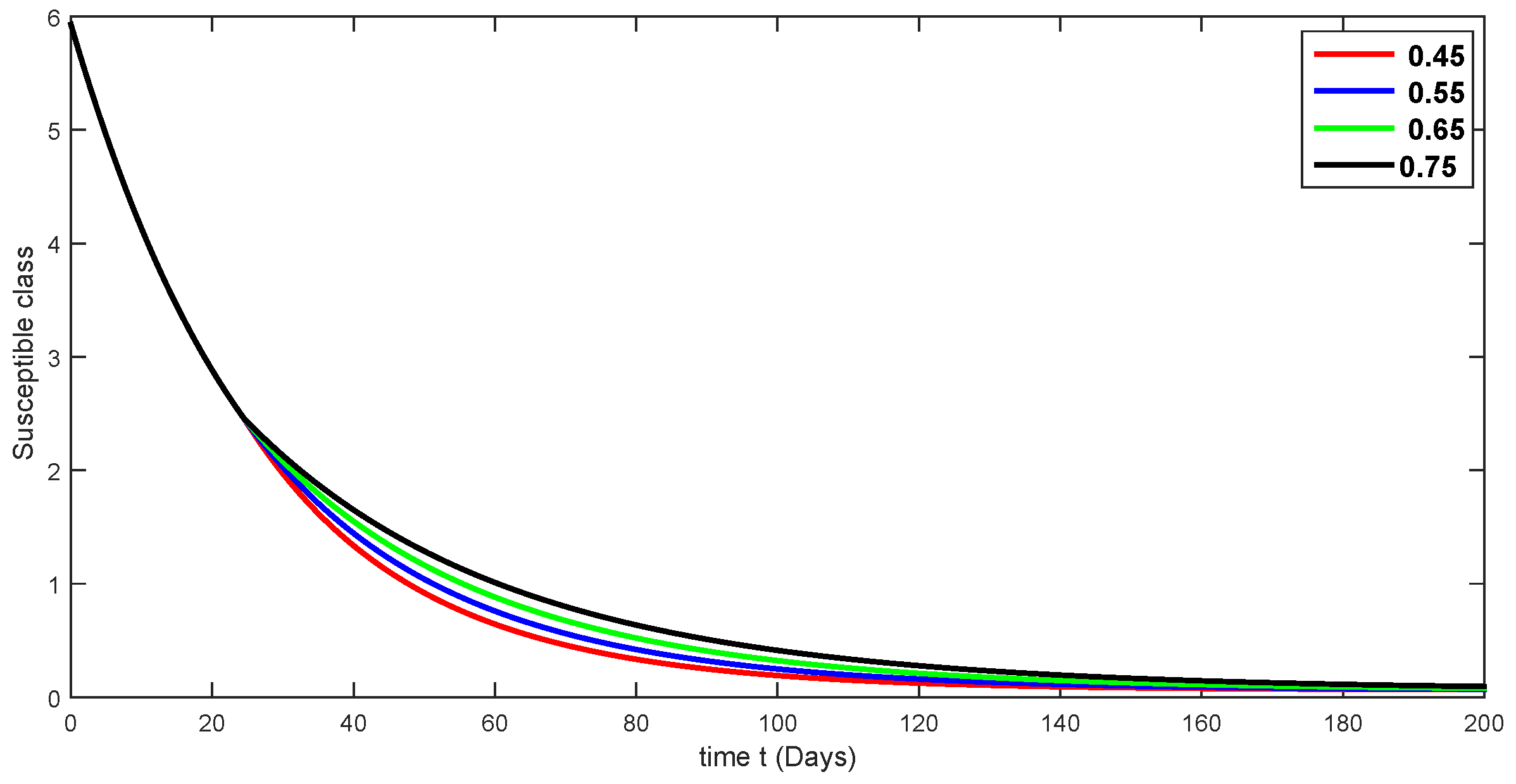
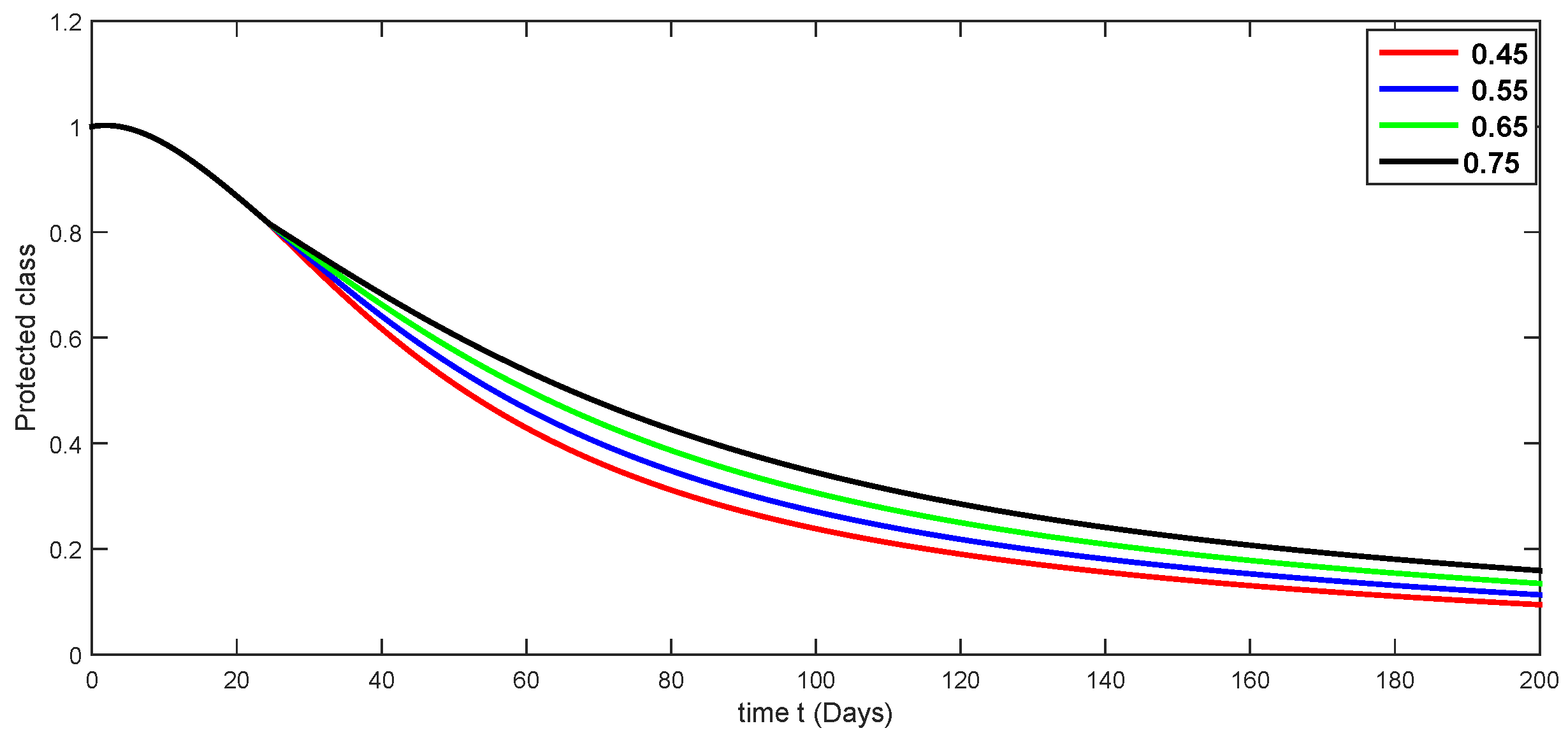
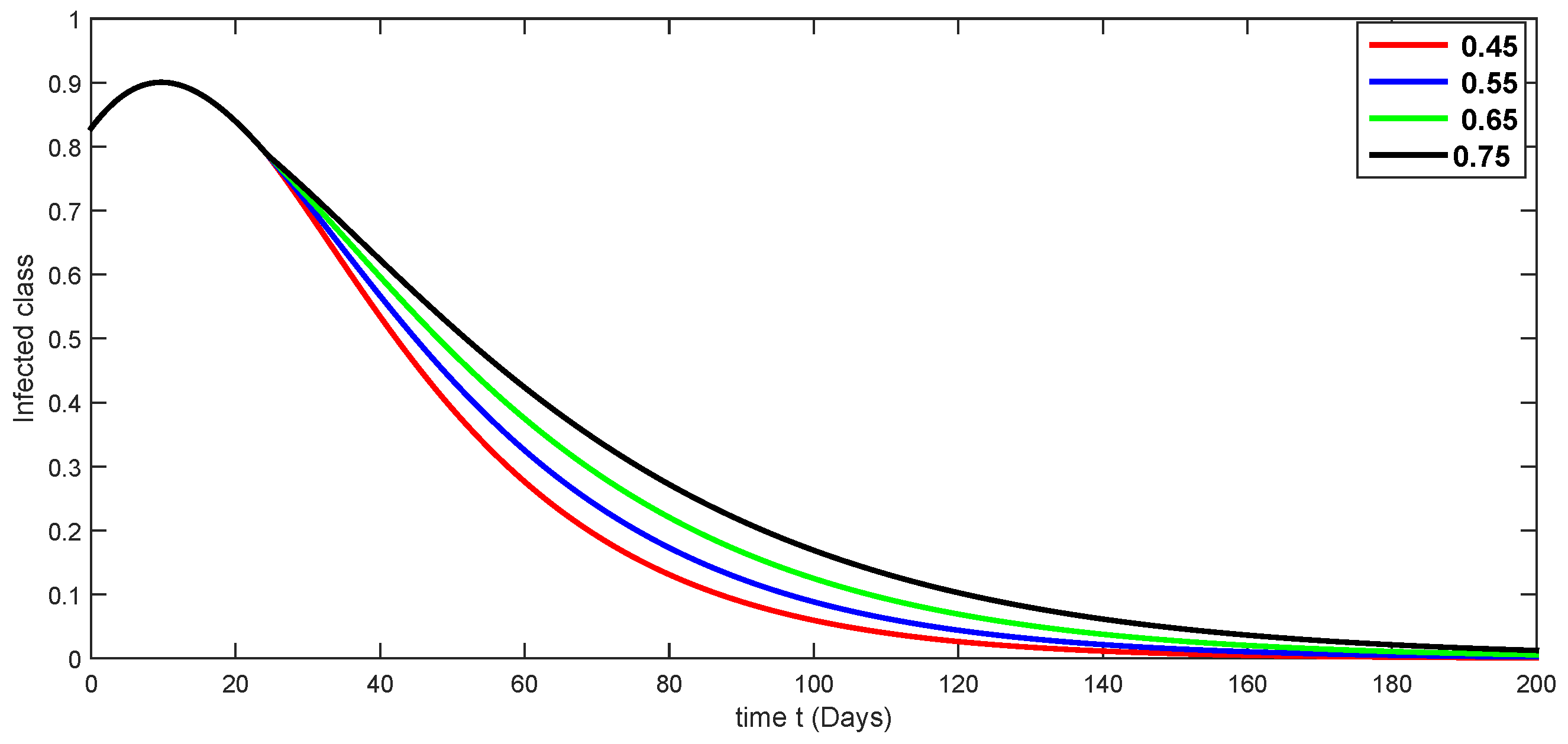
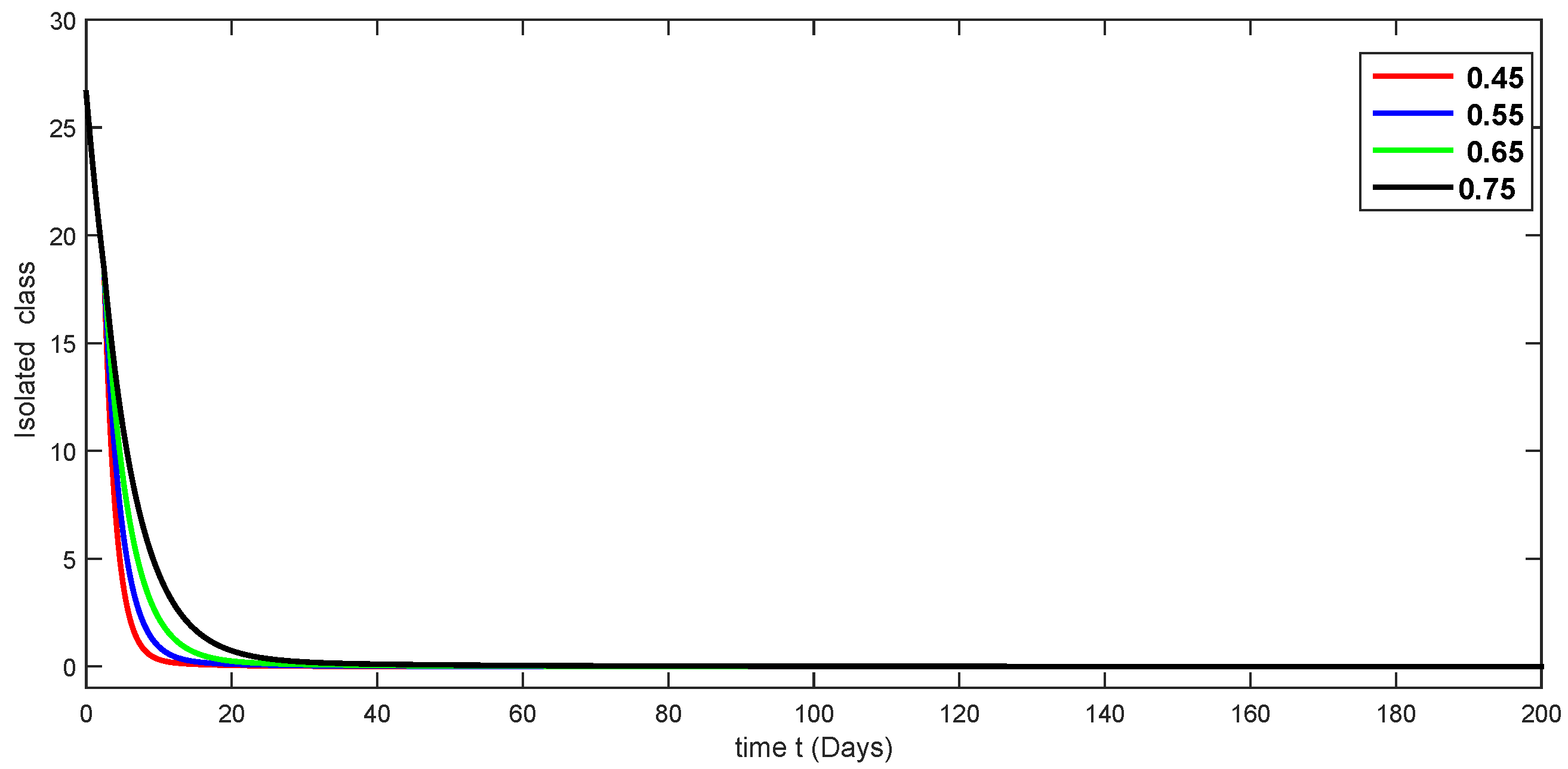
The proposed model’s solution will be unique in relation to these data, meeting the requirements of Theorem 2. The results devoted to numerical interpretations against various fractional-order values for two different sets are displayed in Figure 3, Figure 4, Figure 5, Figure 6, Figure 7, Figure 8 and Figure 9 and Figure 10, Figure 11, Figure 12, Figure 13, Figure 14, Figure 15 and Figure 16, respectively.
In the next set of figures, Figure 10, Figure 11, Figure 12, Figure 13, Figure 14, Figure 15 and Figure 16, we present another set of piecewise fractional-order dynamics of the proposed model. Here, we present the numerical solutions for different classes using a fractional order that lies in ( 0.75 , 1.00 ] .

6. Numerical Discussion and Comparison with Real Data

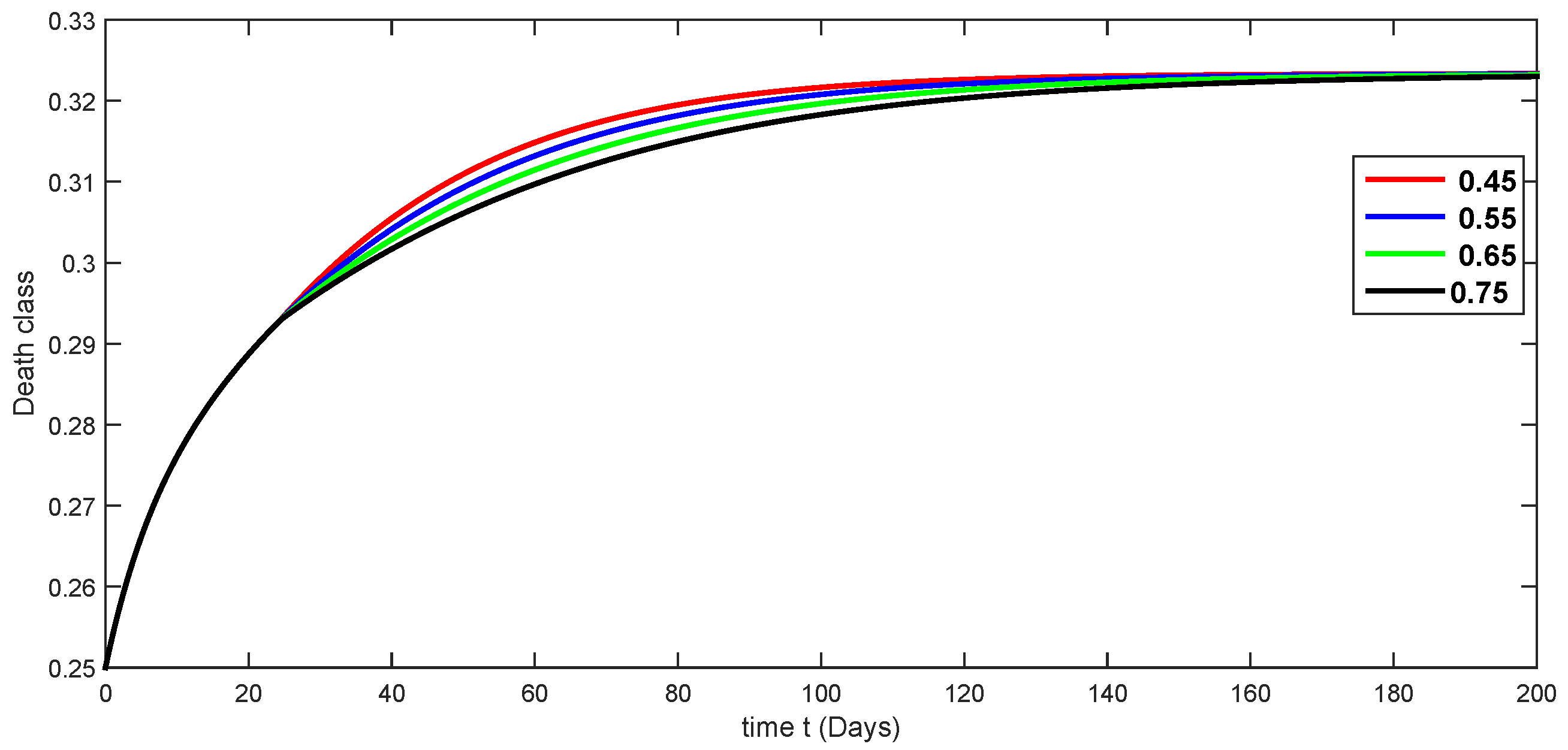
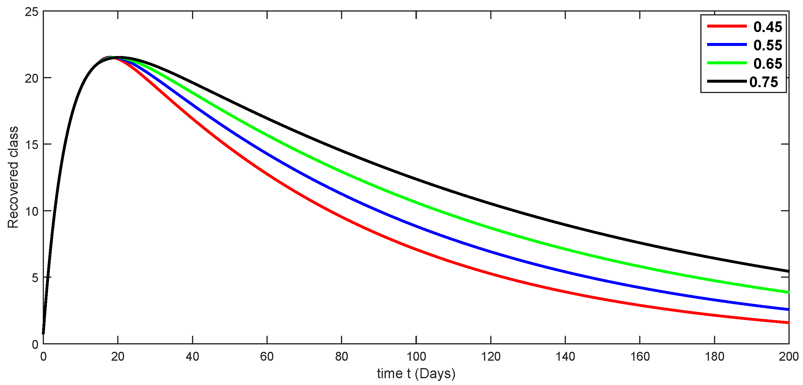
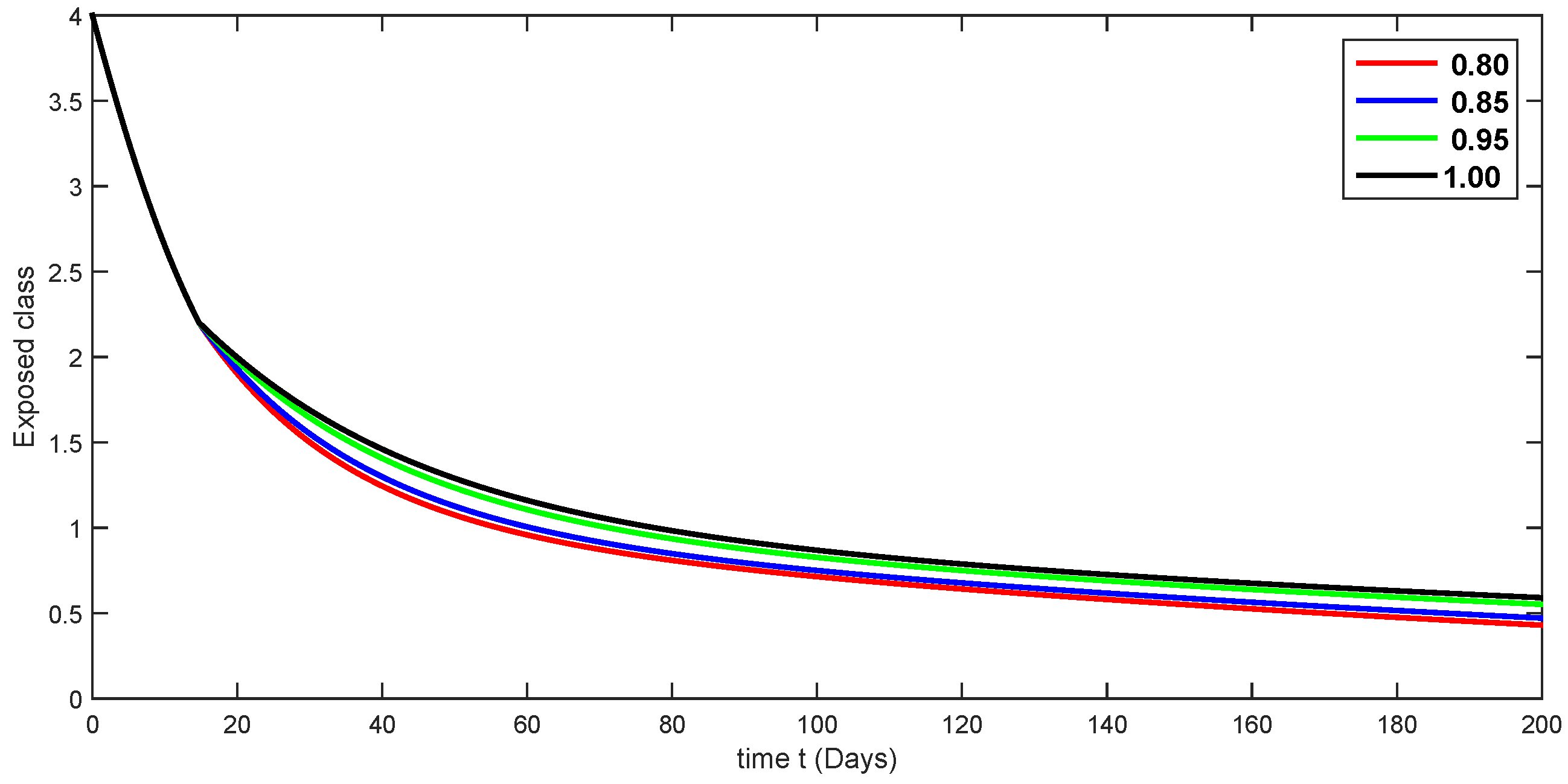
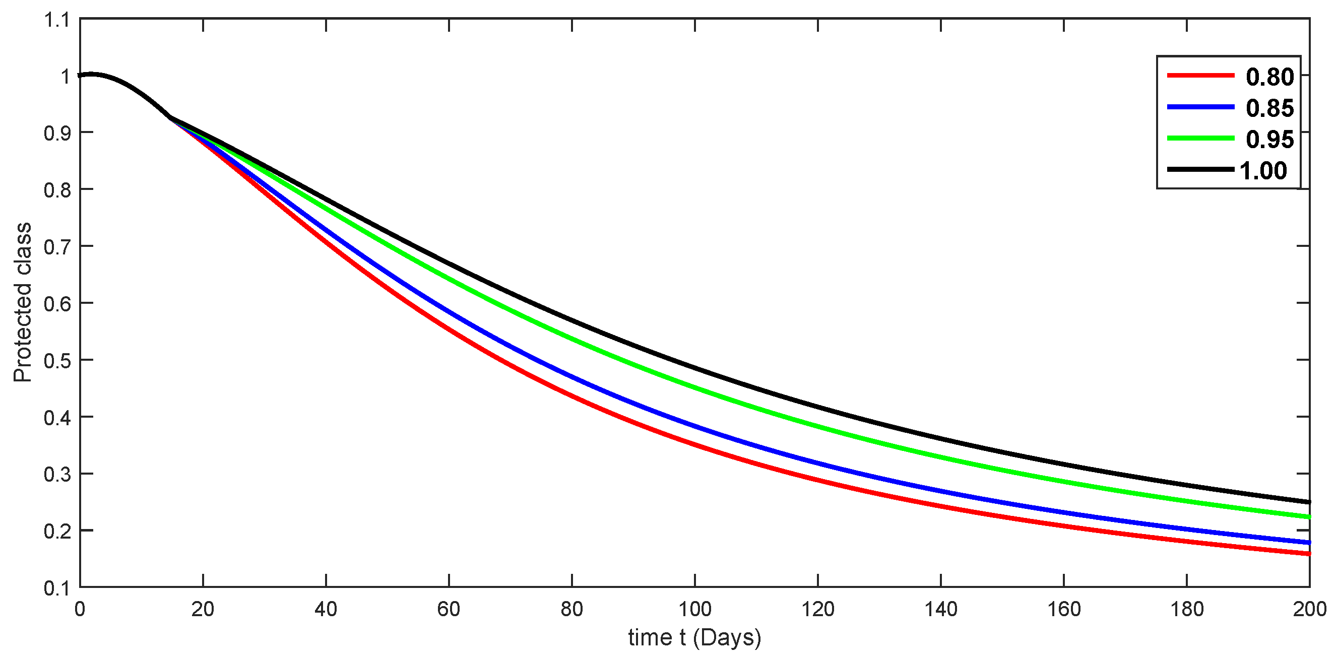
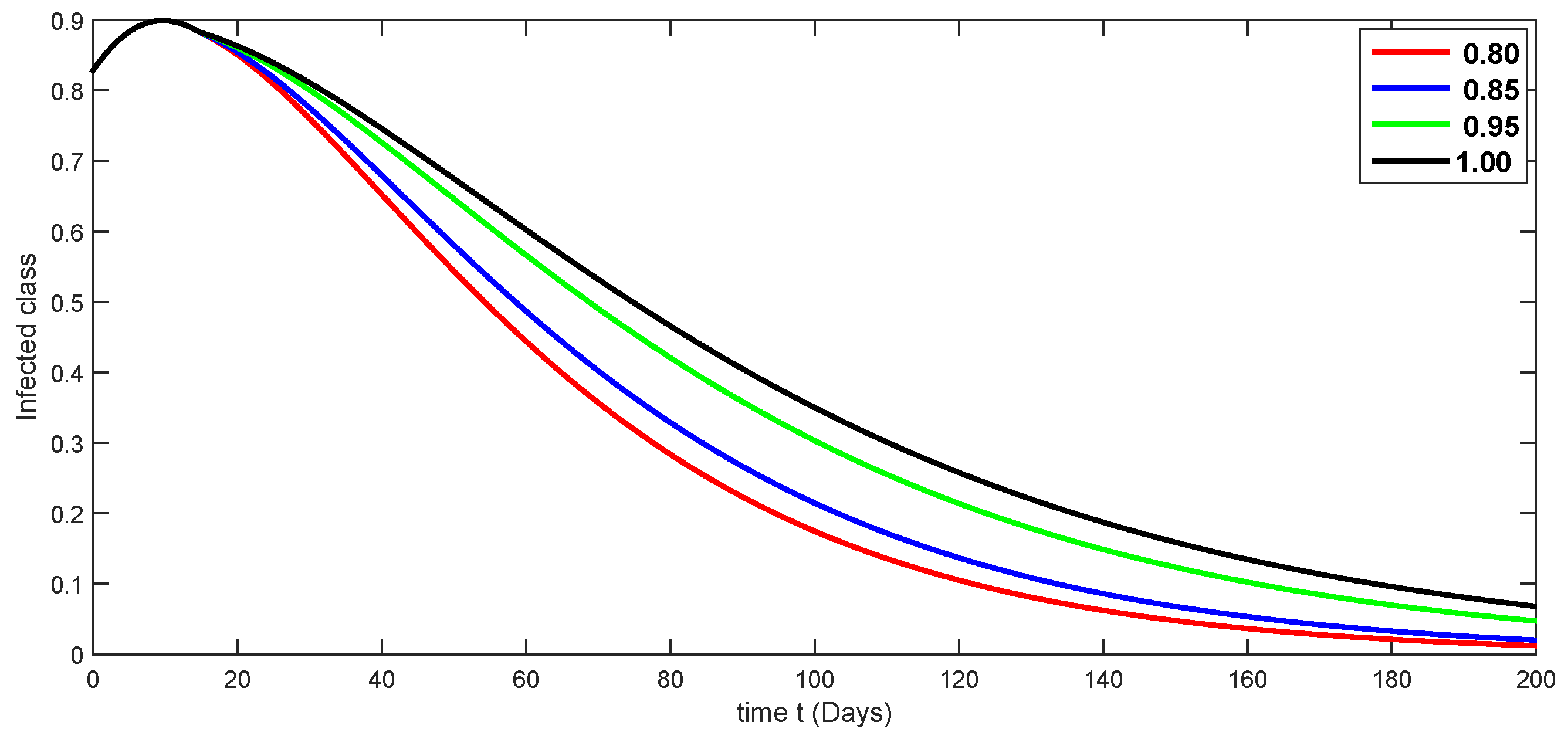
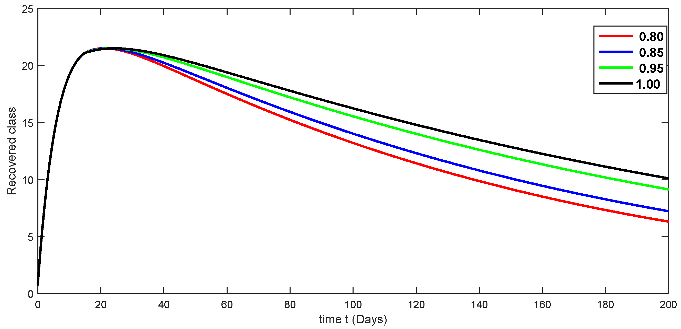
Here, we simulate our model corresponding to piecewise FDEs by varying the fractional orders in Figure 3, Figure 4, Figure 5, Figure 6, Figure 7, Figure 8, Figure 9, Figure 10, Figure 11, Figure 12, Figure 13, Figure 14, Figure 15 and Figure 16. In order to see the crossover effect at the specified point t 1 = 20 , we simulate the approximate solutions by picking [ 0 , 20 ] and ( 20 , 200 ] for both compartments of the proposed model. Days are used to measure time here. In this case, we use a fractional order that lies in ( 0 , 0.75 ] to show numerical answers for various classes in Figure 3, Figure 4, Figure 5, Figure 6, Figure 7, Figure 8 and Figure 9. Additionally, in Figure 10, Figure 11, Figure 12, Figure 13, Figure 14, Figure 15 and Figure 16, the numerical results are presented graphically using various fractional-order values from ( 0.75 , 1.00 ] .
A compartmental model for the transmission dynamics of COVID-19, including the death class, was formulated. We used the new perspectives of fractional calculus that was recently introduced by researchers, which has the ability to describe the crossover behaviors of real-world phenomena. We saw that the population dynamics of the susceptible class decreased, and the crossover effect appears after t 1 = 20 , where the multi-phase behavior is clearly seen. The concerned multi-phase or crossover behavior is different due to different fractional orders. In the same way, the protected class is also decreasing with the crossover behavior after t 1 = 20 , since the density of the pretesting population is decreasing as infection in the society grows. Also, the crossover behavior can be seen near t 1 = 20 in the infected class. The infection, after achieving its peak, is then decreasing. The numbers of isolated and quarantined people are also decreasing as the number of recovered people is growing. Also, the recovery rate is faster, but the death number is also increasing until it becomes stable. In both mentioned classes, the crossover effect appears after t 1 = 20 . The proposed model provides us a better indication of the COVID-19 situation using the new aspect of fractional calculus.
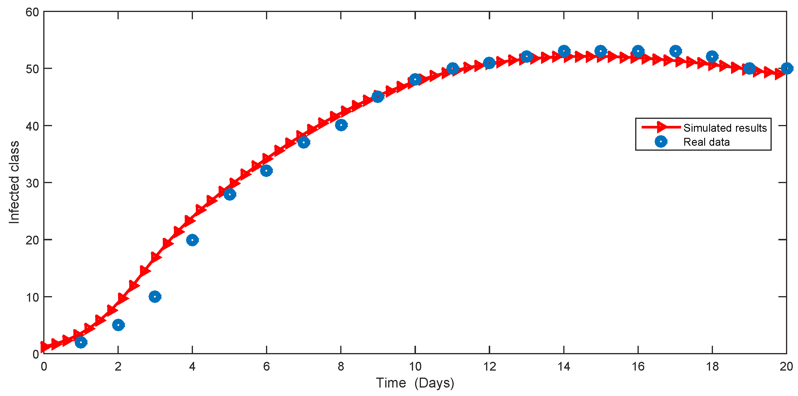
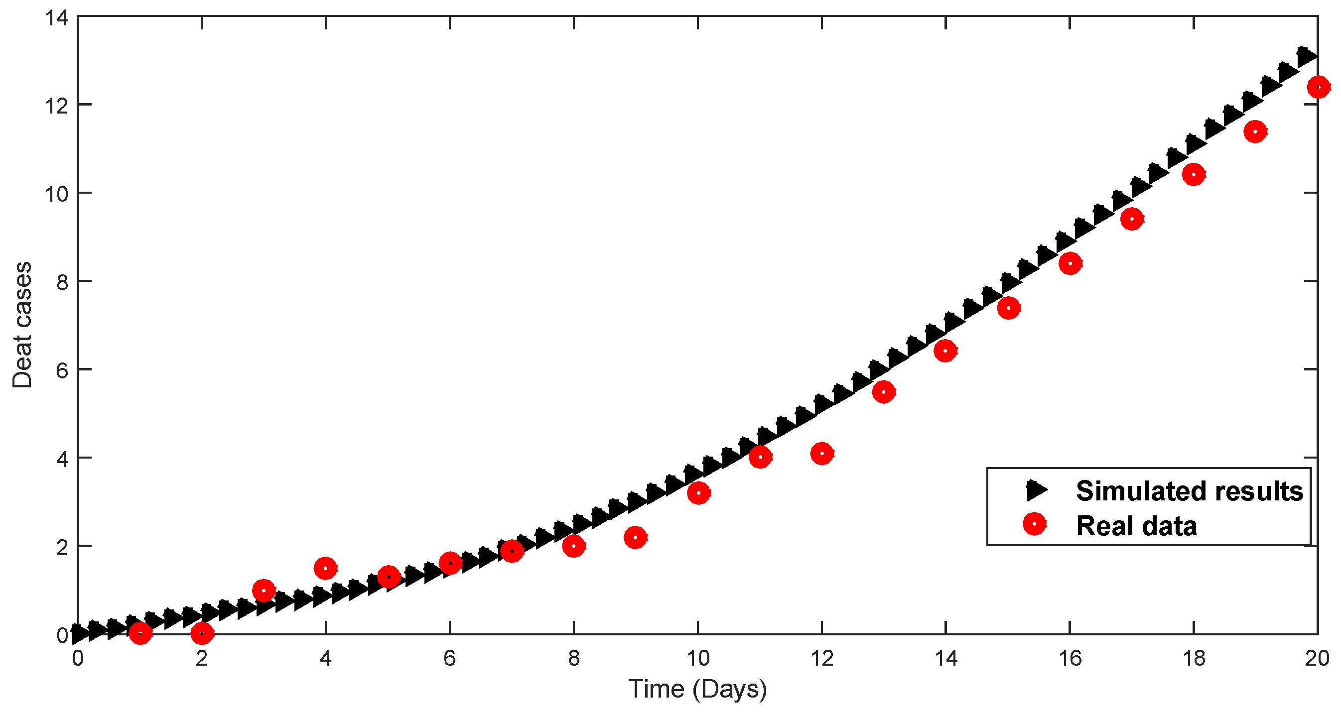
To demonstrate the validity of a numerical scheme for the considered non-linear model of COVID-19, we compared our results with some reported data of death and infected classes. We compared our simulated results for 20 days with the reported data of Pakistan during 2021 using the source [31] for infected and death cases. We performed the comparison to verify the validity of the numerical scheme adopted for the proposed model. Both results have close agreement, as shown in Figure 17 and Figure 18, respectively.

7. Conclusions

Crossover tendencies are observed in a wide range of real-world processes and phenomena. We know that different kernels exhibiting behaviors that arise in various real-world problems can be excellently described by applying the concept of piecewise differential operators. Fluctuations are appearing in many real world process, for instance, the economies of less developed countries and the health system, and weather conditions in many areas are some examples, where the natural processes can give birth to crossover behavior in their state of evolution. To model such phenomena more realistically, the piecewise differential and integral operators of fractional orders were recently introduced. Researchers have increasingly studied various diseases using mathematical models involving piecewise differential operators. Usually, the published work has been based on numerical analysis since mathematical analysis is a powerful area to be used to investigate the existence theory of solutions to such mathematical models and their numerical interpretations.
The fractional-order epidemic model (4) under piecewise equations with fractional-order derivative was thoroughly studied in this work. We created adequate prerequisites for the originality and existence of the suggested problem’s solution. Then, we established an appropriate scheme based on the Adam–Bashforth method. We then simulated the considered model using various fractional-order values, taking t 1 = 20 and T = 200 . The corresponding dynamics were shown with clear crossover behavior near t 1 = 20 . Hence, we concluded that piecewise equations with fractional-order derivative are powerful tools for describing abrupt changes in the dynamics of various evolutionary processes and phenomena. We compared some results with the available reported data of infected and death classes to check the efficiency of the adopted numerical scheme. In the future, we will extend this concept to other dynamical problems with various fractional-order operators.

Author Contributions

Methodology, M.R.; Formal analysis, Z.A.K.; Data curation, S.A. and A.A.A.; writing—original draft preparation, M.R.; Writing—review & editing, S.A. and A.A.A. All authors have read and agreed to the published version of the manuscript.

Funding

This research was supported by EIAS Data Science & Blockchain Lab, Prince Sultan University. The authors would like to thank Prince Sultan University for paying the APC of this article.

Data Availability Statement

Data is contained within the article.

Acknowledgments

The authors thank Princess Nourah bint Abdulrahman University Researchers Supporting Project number (PNURSP2024R8) and Princess Nourah bint Abdulrahman University, Riyadh, Saudi Arabia. The authors would like to thank Prince Sultan University for their support.

Conflicts of Interest

The authors declare no conflicts of interest.

References

  1. Ross, R. An application of the theory of probabilities to the study of a priori pathometry-Part I. Proc. R. Soc. Lond. Ser. A Contain. Pap. Math. Phys. Character 1916, 92, 204–230. [Google Scholar]
  2. Ross, R.; Hudson, H.P. An application of the theory of probabilities to the study of a priori pathometry Part II. Proc. R. Soc. Lond. Ser. A Contain. Pap. Math. Phys. Character 1917, 93, 212–225. [Google Scholar]
  3. Kermack, W.O.; McKendrick, A.G. A contribution to the mathematical theory of epidemics. Proc. R. Soc. Lond. Ser. A Contain. Pap. Math. Phys. Character 1927, 115, 700–721. [Google Scholar]
  4. La Salle, J.P. The Stability of Dynamical Systems; Society for Industrial and Applied Mathematics: Philadelphia, PA, USA, 1976. [Google Scholar]
  5. Korobeinikov, A. Global properties of basic virus dynamics models. Bull. Math. Biol. 2004, 66, 879–883. [Google Scholar] [CrossRef] [PubMed]
  6. Patel, P.; Borkowf, C.B.; Brooks, J.T.; Lasry, A.; Lansky, A.; Mermin, J. Estimating per-act HIV transmission risk: A systematic review. AIDS 2014, 28, 1509. [Google Scholar] [CrossRef]
  7. Munch, Z.; Van Lill, S.W.P.; Booysen, C.N.; Zietsman, H.L.; Enarson, D.A.; Beyers, N. Tuberculosis transmission patterns in a high-incidence area: A spatial analysis. Int. J. Tuberc. Lung Dis. 2003, 7, 271–277. [Google Scholar] [PubMed]
  8. Nuno, M.; Castillo-Chavez, C.; Feng, Z.; Martcheva, M. Mathematical models of influenza: The role of cross-immunity, quarantine and age-structure. In Mathematical Epidemiology; Springer: Berlin/Heidelberg, Germany, 2008; pp. 349–364. [Google Scholar]
  9. Schaffner, F.; Mathis, A. Dengue and dengue vectors in the WHO European region: Past, present, and scenarios for the future. Lancet Infect. Dis. 2014, 14, 1271–1280. [Google Scholar] [CrossRef]
  10. Agusto, F.B.; Adekunle, A.I. Optimal control of a two-strain tuberculosis-HIV/AIDS co-infection model. Biosystems 2014, 119, 20–44. [Google Scholar] [CrossRef] [PubMed]
  11. Forouzannia, F.; Gumel, A. Dynamics of an age-structured two-strain model for malaria transmission. Appl. Math. Comput. 2015, 250, 860–886. [Google Scholar] [CrossRef]
  12. Atangana, A.; Araz, S.I. New concept in calculus: Piecewise differential and integral operators. Chaos Solitons Fractals 2021, 145, 110638. [Google Scholar] [CrossRef]
  13. Ross, B. A brief history and exposition of the fundamental theory of fractional calculus. In Fractional Calculus and Its Applications; Springer: Berlin/Heidelberg, Germany, 1975; pp. 1–36. [Google Scholar]
  14. Baba, I.A.; Hincal, E. Global stability analysis of two-strain epidemic model with bilinear and non-monotone incidence rates. Eur. Phys. J. Plus 2017, 132, 208. [Google Scholar] [CrossRef]
  15. Baba, I.A.; Hincal, E.; Alsaadi, S.H.K. Global stability analysis of a two strain epidemic model with awareness. Adv. Differ. Equ. Control Process. 2018, 19, 83–100. [Google Scholar] [CrossRef]
  16. Bentaleb, D.; Amine, S. Lyapunov function and global stability for a two-strain SEIR model with bilinear and non-monotone incidence. Int. J. Biomath. 2019, 12, 1950021. [Google Scholar] [CrossRef]
  17. Meskaf, A.; Khyar, O.; Danane, J.; Allali, K. Global stability analysis of a two-strain epidemic model with non-monotone incidence rates. Chaos Solitons Fractals 2020, 133, 109647. [Google Scholar] [CrossRef]
  18. Ouncharoen, R.; Shah, K.; Ud Din, R.; Abdeljawad, T.; Ahmadian, A.; Salahshour, S.; Sitthiwirattham, T. Study of integer and fractional order COVID-19 mathematical model. Fractals 2020, 31, 2340046. [Google Scholar] [CrossRef]
  19. Arfan, M.; Shah, K.; Abdeljawad, T.; Mlaiki, N.; Ullah, A. A Caputo power law model predicting the spread of the COVID-19 outbreak in Pakistan. Alex. Eng. J. 2021, 60, 447–456. [Google Scholar] [CrossRef]
  20. Tuan, N.H.; Mohammadi, H.; Rezapour, S. A mathematical model for COVID-19 transmission by using the Caputo fractional derivative. Chaos Solitons Fractals 2020, 140, 110107. [Google Scholar] [CrossRef] [PubMed]
  21. Roccetti, M. Drawing a parallel between the trend of confirmed COVID-19 deaths in the winters of 2022/2023 and 2023/2024 in Italy, with a prediction. Math. Biosci. Eng. 2024, 21, 3742–3754. [Google Scholar] [CrossRef]
  22. Khan, S.; Khan, Z.A.; Alrabaiah, H.; Zeb, S. On using piecewise fractional differential operator to study a dynamical system. Axioms 2023, 12, 292. [Google Scholar] [CrossRef]
  23. Alharthi, N.H.; Jeelani, M.B. Study of Rotavirus Mathematical Model Using Stochastic and Piecewise Fractional Differential Operators. Axioms 2023, 12, 970. [Google Scholar] [CrossRef]
  24. Nisar, K.S.; Farman, M.; Jamil, K.; Akgül, A.; Jamil, S. Computational and stability analysis of Ebola virus epidemic model with piecewise hybrid fractional operator. PLoS ONE 2024, 19, e0298620. [Google Scholar] [CrossRef] [PubMed]
  25. Redhwan, S.S.; Han, M.; Almalahi, M.A.; Alyami, M.A.; Alsulami, M.; Alghamdi, N. Piecewise implicit coupled system under ABC fractional differential equations with variable order. AIMS Math. 2024, 9, 15303–15324. [Google Scholar] [CrossRef]
  26. Khan, S.; Shah, K.; Debbouche, A.; Zeb, S.; Antonov, V. Solvability and Ulam-Hyers stability analysis for nonlinear piecewise fractional cancer dynamic systems. Phys. Scr. 2024, 99, 025225. [Google Scholar] [CrossRef]
  27. Riaz, M.; Shah, K.; Ullah, A.; Alqudah, M.A.; Abdeljawad, T. The Volterra-Lyapunov matrix theory and nonstandard finite difference scheme to study a dynamical system. Results Phys. 2023, 52, 106890. [Google Scholar] [CrossRef]
  28. Shah, K.; Khan, A.; Abdalla, B.; Abdeljawad, T.; Khan, K.A. A mathematical model for Nipah virus disease by using piecewise fractional order Caputo derivative. Fractals 2024, 32, 2440013. [Google Scholar] [CrossRef]
  29. Atangana, A.; Araz, S.I. Piecewise differential equations: Theory, methods and applications. AIMS Math. 2023, 8, 15352–15382. [Google Scholar] [CrossRef]
  30. Atangana, A. Mathematical model of survival of fractional calculus, critics and their impact: How singular is our world? Adv. Differ. Equ. 2021, 2021, 403. [Google Scholar] [CrossRef]
  31. 2021. Available online: https://www.worldometers.info/coronavirus/country/pakistan/ (accessed on 13 April 2024).
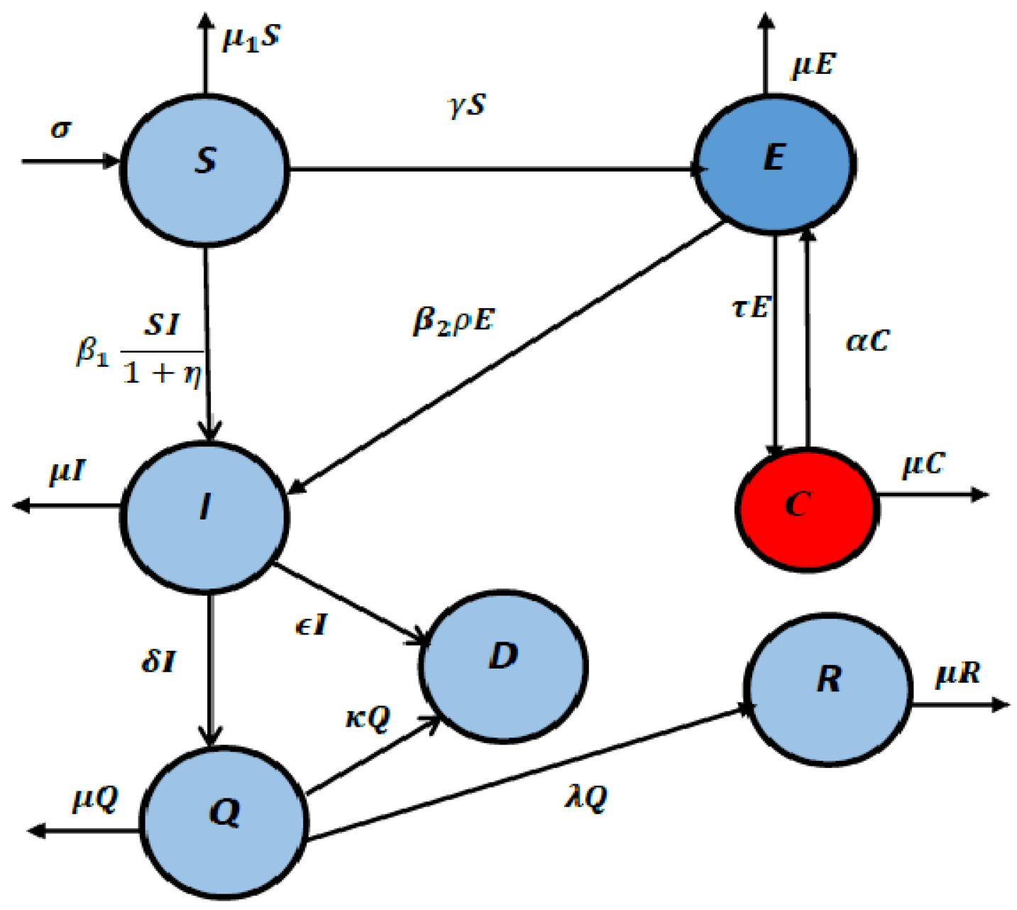
Figure 1. Schematic flowchart of model (24).
Fractalfract 08 00291 g001
Figure 2. Three-dimensional representations of R 0 .
Fractalfract 08 00291 g002
Figure 3. Fractional-order dynamical behaviors of the susceptible class of the proposed model (4) using various fractional-order values in ( 0 , 0.75 ] .
Fractalfract 08 00291 g003
Figure 4. Fractional-order dynamical behaviors of the exposed class of the proposed model (4) using various fractional-order values in ( 0 , 0.75 ] .
Fractalfract 08 00291 g004
Figure 5. Fractional-order dynamical behaviors of the protected class of the proposed model (4) using various fractional-order values in ( 0 , 0.75 ] .
Fractalfract 08 00291 g005
Figure 6. Fractional-order dynamical behaviors of the infected class of the proposed model (4) using various fractional-order values in ( 0 , 0.75 ] .
Fractalfract 08 00291 g006
Figure 7. Fractional-order dynamical behaviors of the isolated class of the proposed model (4) using various fractional-order values in ( 0 , 0.75 ] .
Fractalfract 08 00291 g007
Figure 8. Fractional-order dynamical behaviors of the death class of the proposed model (4) using various fractional-order values in ( 0 , 0.75 ] .
Fractalfract 08 00291 g008
Figure 9. Fractional-orde r dynamical behaviors of the recovered class of the proposed model (4) using various fractional-order values in ( 0 , 0.75 ] .
Fractalfract 08 00291 g009
Figure 10. Fractional-order dynamical behaviors of the susceptible class of the proposed model (4) using various fractional-order values in ( 0.75 , 1.00 ] .
Fractalfract 08 00291 g010
Figure 11. Fractional-order dynamical behaviors of the exposed class of the proposed model (4) using various fractional-order values in ( 0.75 , 1.00 ] .
Fractalfract 08 00291 g011
Figure 12. Fractional-order dynamical behaviors of the protected class of the proposed model (4) using various fractional-order values in ( 0.75 , 1.00 ] .
Fractalfract 08 00291 g012
Figure 13. Fractional-order dynamical behaviors of the infected class of the proposed model (4) using various fractional-order values in ( 0.75 , 1.00 ] .
Fractalfract 08 00291 g013
Figure 14. Fractional-order dynamical behaviors of the isolated class of the proposed model (4) using various fractional-order values in ( 0.75 , 1.00 ] .
Fractalfract 08 00291 g014
Figure 15. Fractional-order dynamical behaviors of the death class of the proposed model (4) using various fractional-order values in ( 0.75 , 1.00 ] .
Fractalfract 08 00291 g015
Figure 16. Fractional-order dynamical behaviors of the recovered class of the proposed model (4) using various fractional-order values in ( 0.75 , 1.00 ] .
Fractalfract 08 00291 g016
Figure 17. Comparison of real and simulated data in case of infected class.
Fractalfract 08 00291 g017
Figure 18. Comparison of real and simulated data in case of death class.
Fractalfract 08 00291 g018
Table 1. Description of compartments and nomenclature of model (2).
NomenclatureDescription
SSusceptible (the individuals at risk of being affected)
CProtected class (individuals without infection and showing no symptoms)
EExposed (Potentially affected class)
IInfected class
QIsolated class
DDeath class
RRecovered class
μ Rate of natural mortality
σ The rate of immigration into S
η Saturation threshold
δ Isolation rate
α Rate of protective measures
β 1 The rate of disease transmission through contact
β 2 Infectivity rate
γ Rate of immigration from S to E
kViral mortality rate
λ Rate of recovery from Q
τ Duration of protection
ϵ Mortality rate from infection
Table 2. These data sources are found in [27].
ParameterNumerical ValuesParameterNumerical Values
μ 0.00992590 α 0.020
σ 0.00200 β 1 0.005
η 0.02330 β 2 0.0714
ϵ 0.00100 γ 0.02202643
ρ 0.1000k0.000123
δ 0.0290 λ 0.13978
τ 0.008 S ( 0 ) 5.93
E ( 0 ) 4.0 C ( 0 ) 1.0
I ( 0 ) 0.828596 Q ( 0 ) 26.60
D ( 0 ) 0.250 R ( 0 ) 0.8160360
Disclaimer/Publisher’s Note: The statements, opinions and data contained in all publications are solely those of the individual author(s) and contributor(s) and not of MDPI and/or the editor(s). MDPI and/or the editor(s) disclaim responsibility for any injury to people or property resulting from any ideas, methods, instructions or products referred to in the content.