
Complementary Metal Oxide Semiconductor Circuit Realization of Inverse Chebyshev Low-Pass Filter of Order (1 + α)

 and
and
Abstract
1. Introduction
2. Design of Inverse Chebyshev Fractional-Order Filter
2.1. Inverse Chebyshev Fractional-Order Filter
2.1.1. Background
2.1.2. Least Square Fitting Function
2.1.3. Stability
2.1.4. Transfer Function Approximation
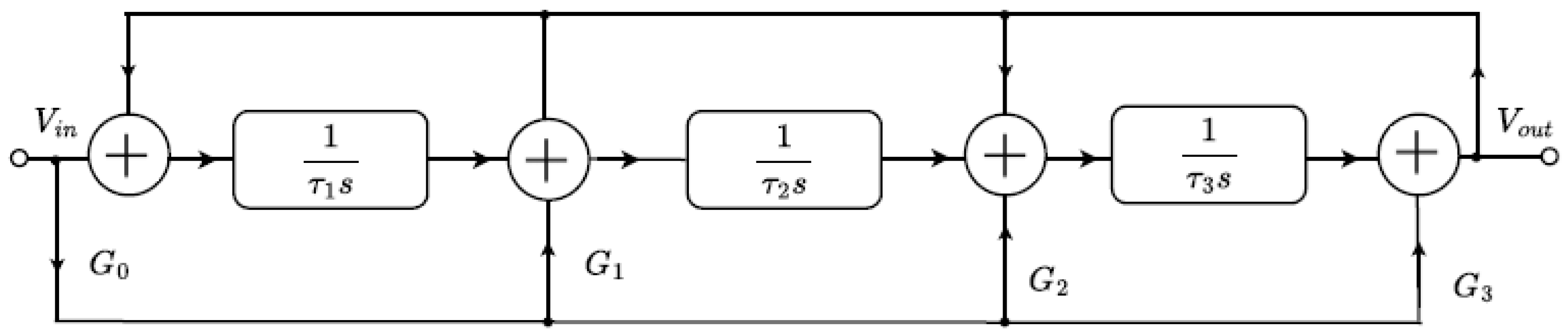
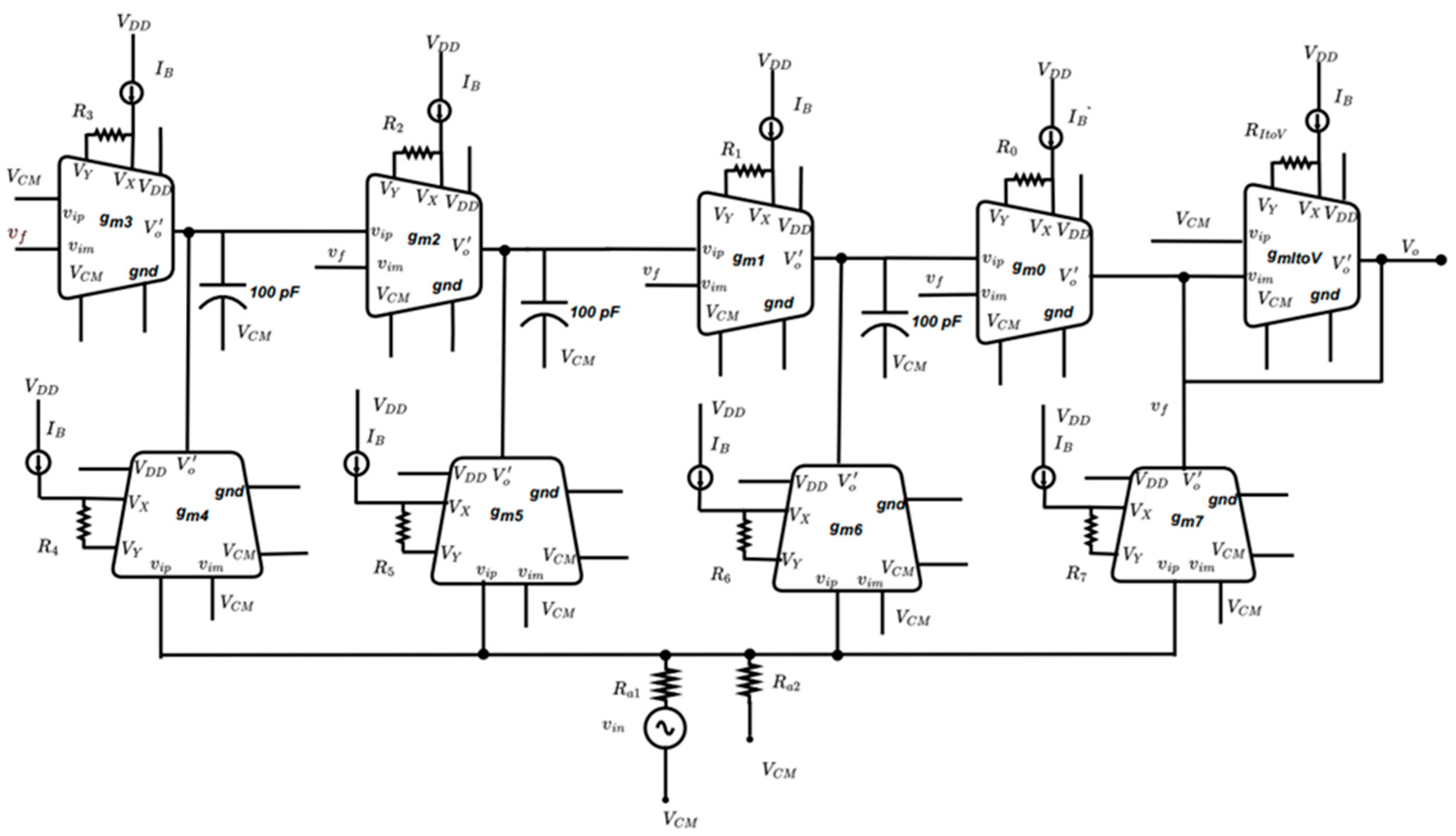
2.1.5. Functional Block Diagram
3. CMOS Circuit Realization of Inverse Chebyshev Fractional-Order Filter
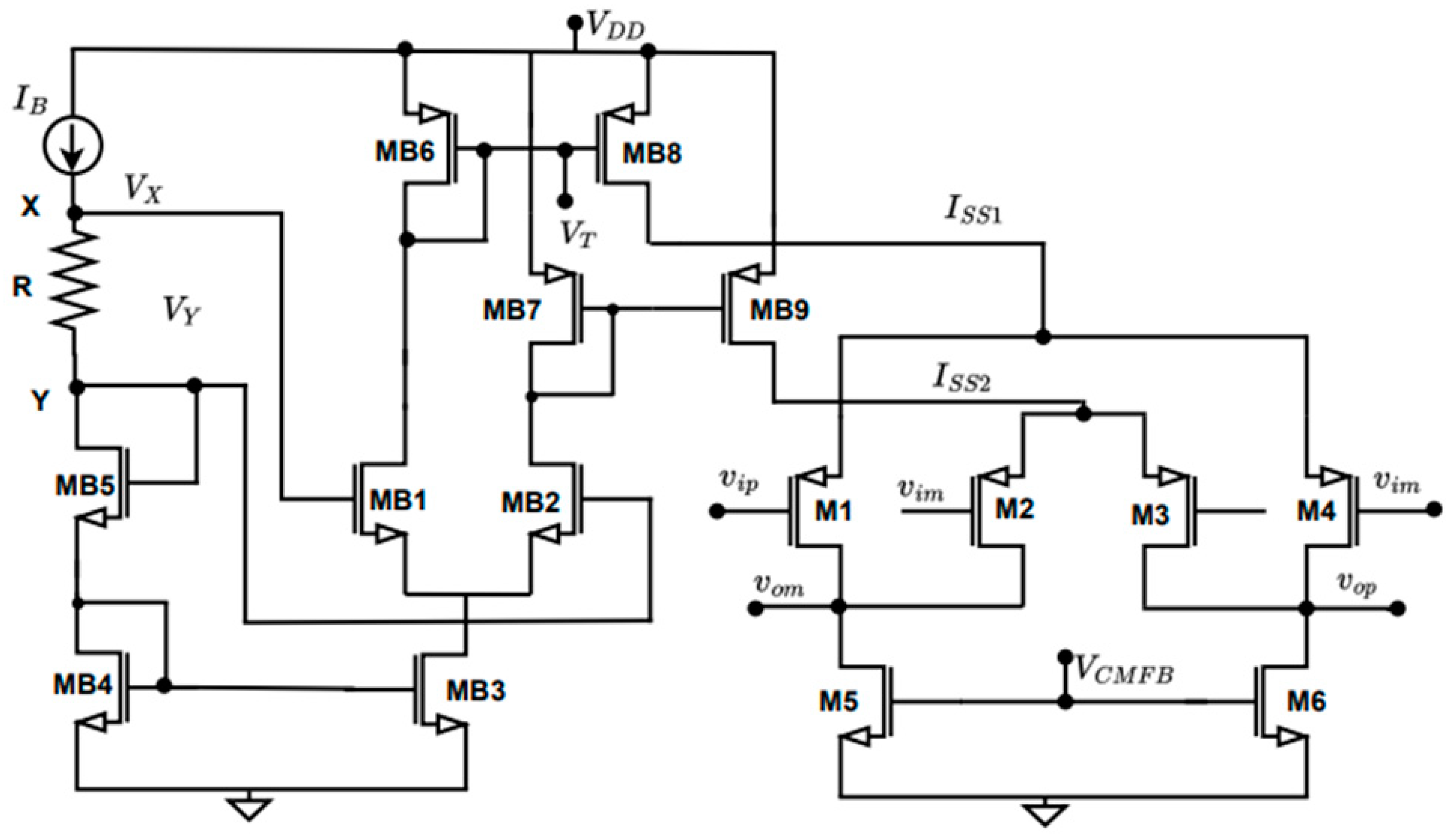
3.1. CMOS OTA Architecture
3.2. Common-Mode Feedback Circuit
4. Simulation Results
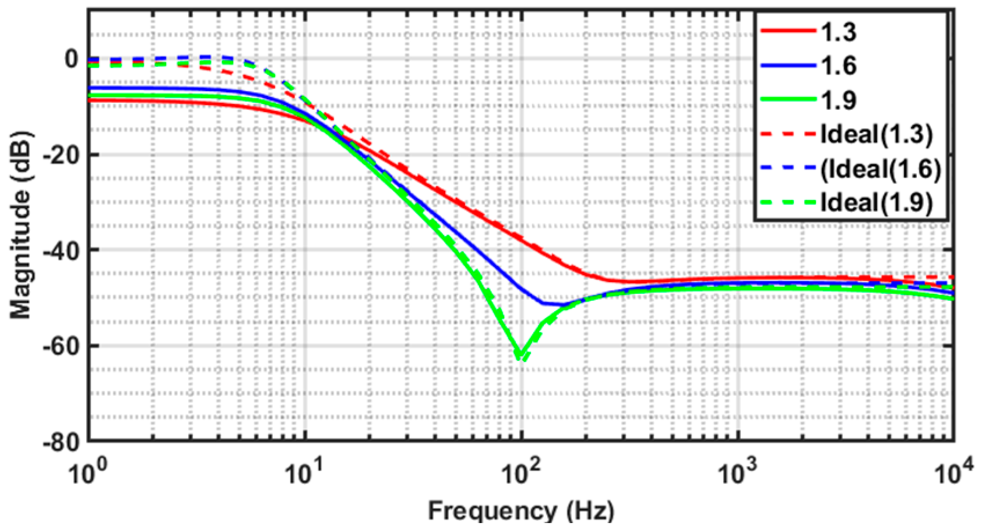
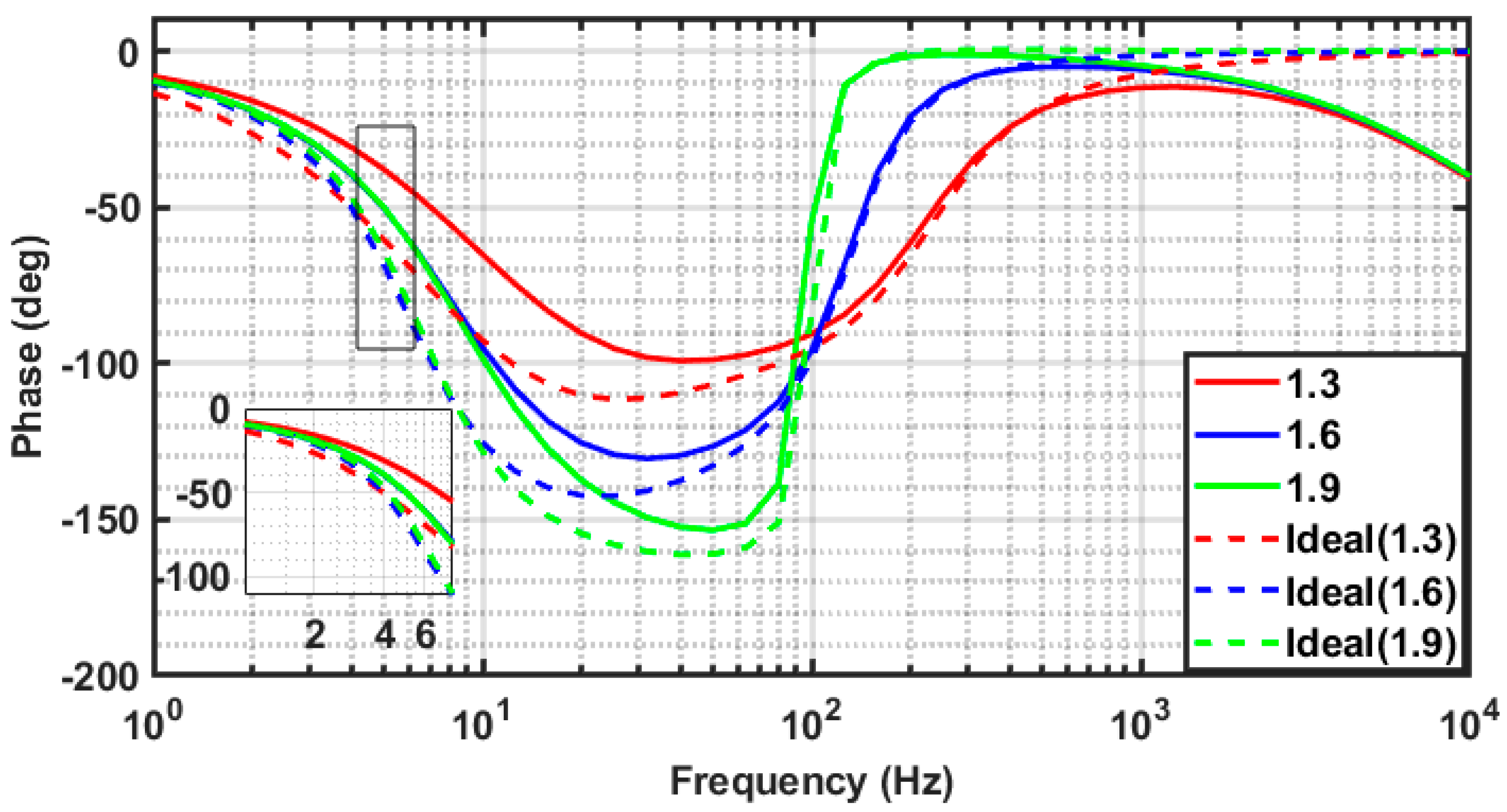
4.1. Amplitude Response
4.2. Transient Characteristics
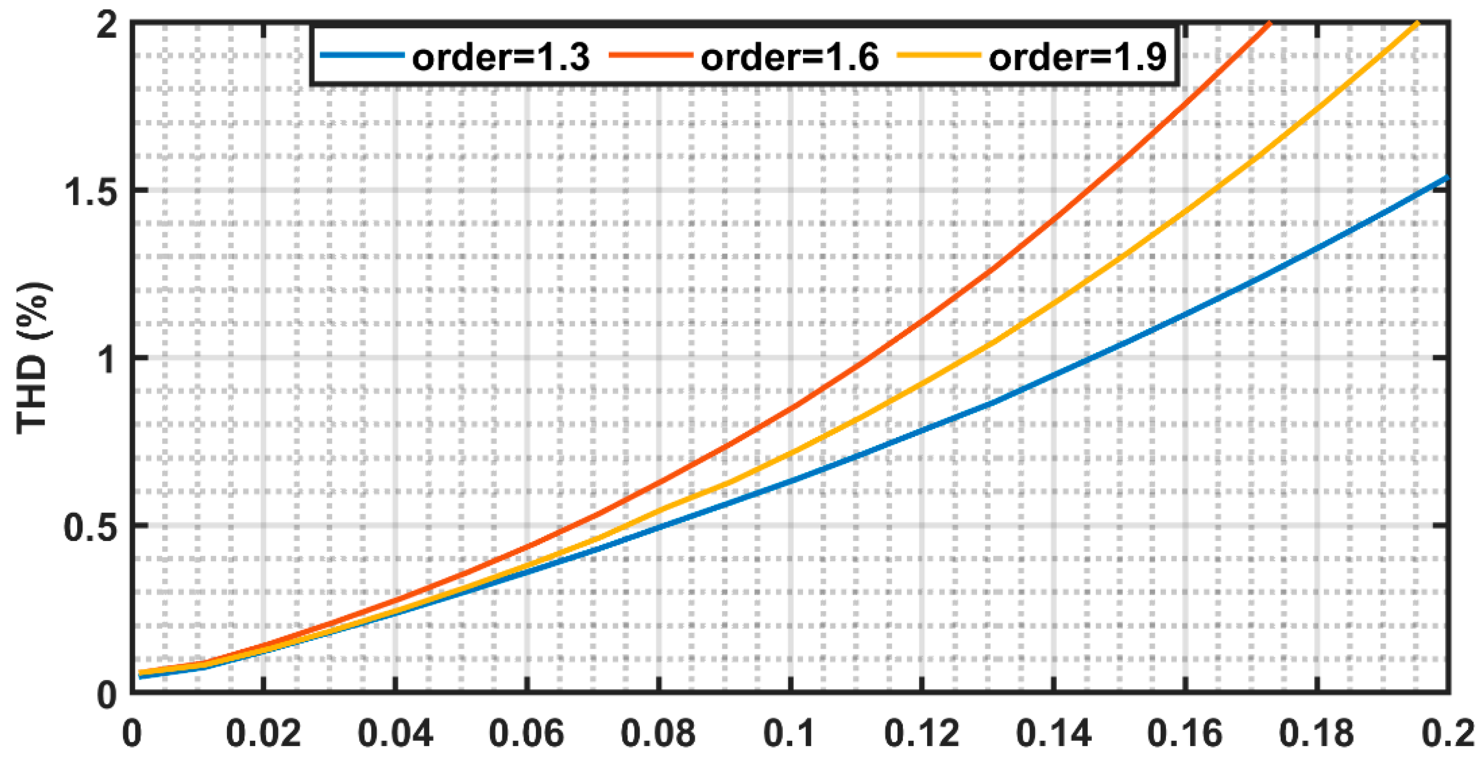
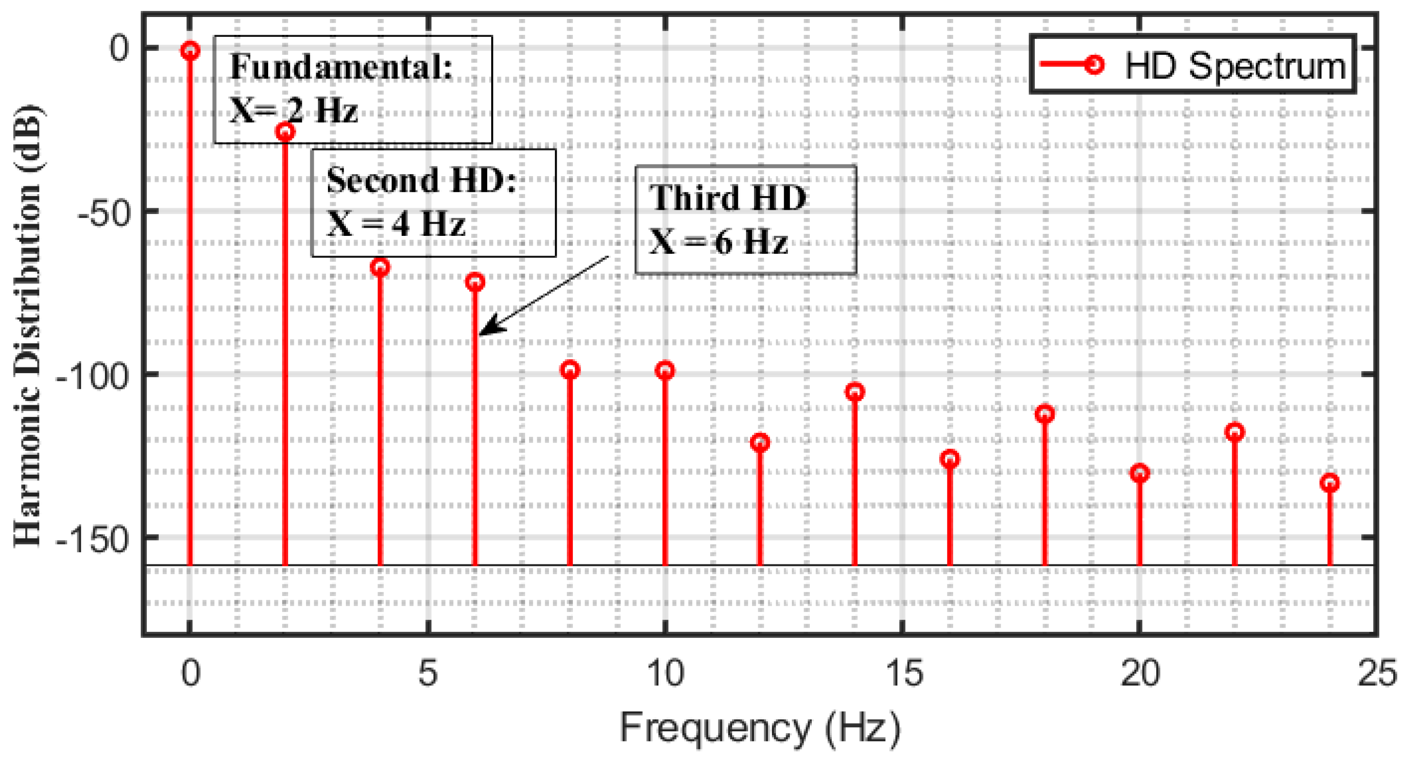
4.3. THD and Harmonic Spectrum
4.4. Monte Carlo Plot
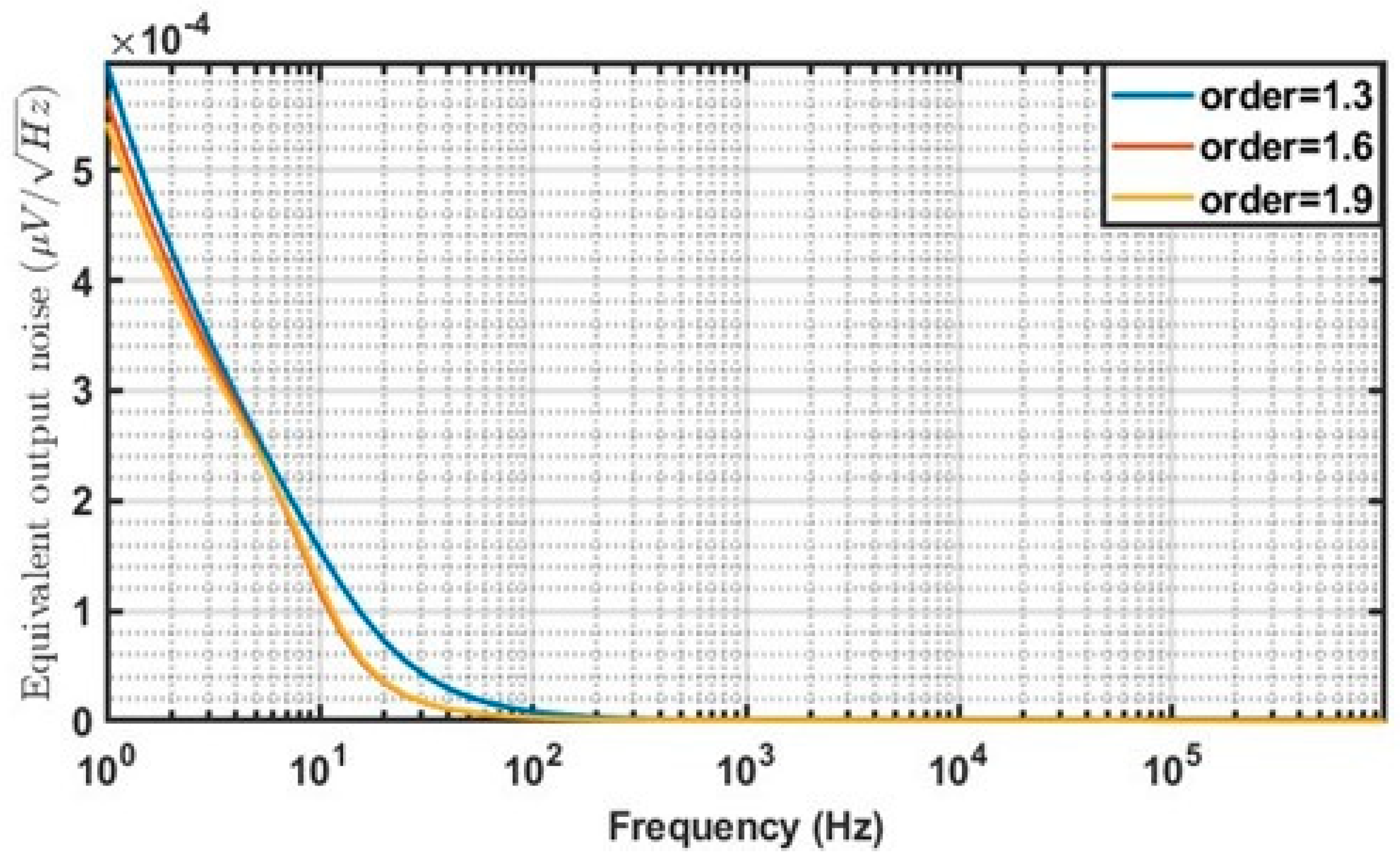
4.5. Output Noise
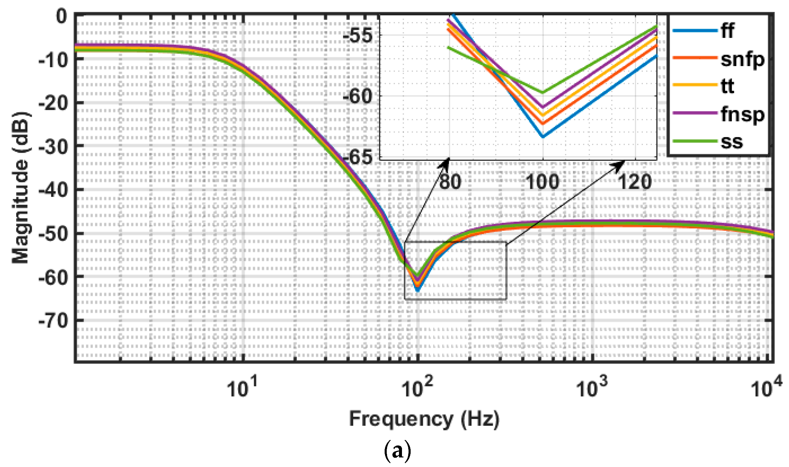
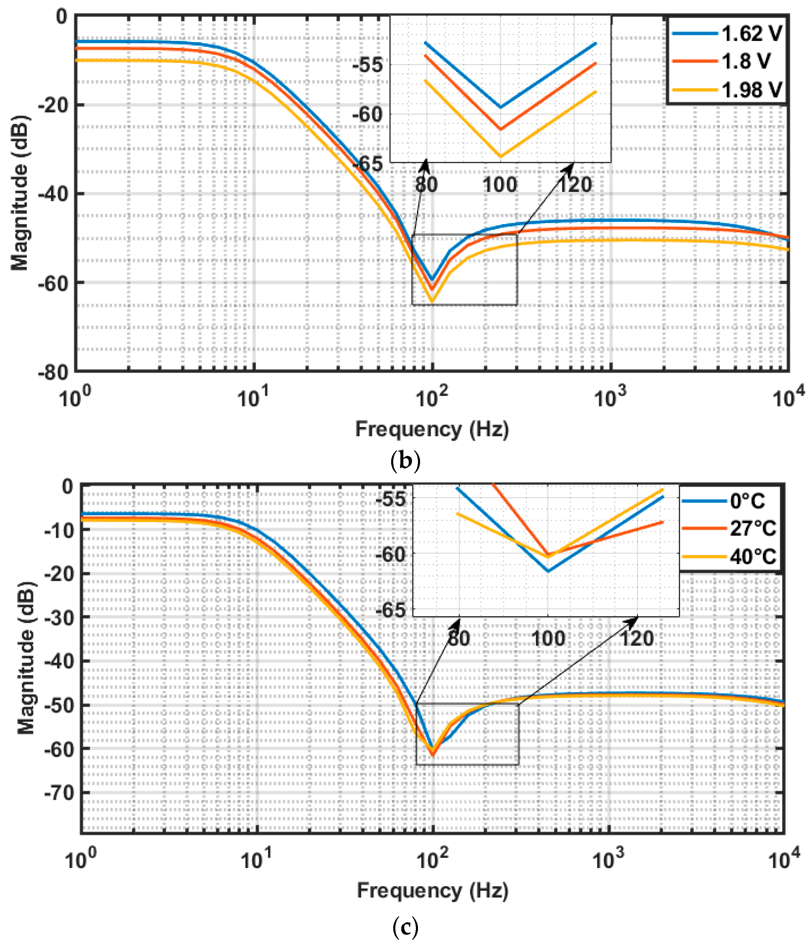
4.6. PVT Plots
5. Performance Evaluation
6. Conclusions
Author Contributions
Funding
Data Availability Statement
Conflicts of Interest
References
- Tsirimokou, G.; Psychalinos, C.; Elwakil, A. Design of CMOS Analog Integrated Fractional-Order Circuits: Applications in Medicine and Biology; Springer: Berlin/Heidelberg, Germany, 2017. [Google Scholar]
- AFreeborn, T.J.; Maundy, B.; Elwakil, A. Fractional Resonance-Based RLβCα Filters. Math. Probl. Eng. 2013, 1, 726721. [Google Scholar] [CrossRef]
- Freeborn, T.J.; Maundy, B.; Elwakil, A.S. Field Programmable Analogue Array Implementation of Fractional Step Filters. IET Circuits Devices Syst. 2010, 4, 514–524. [Google Scholar] [CrossRef]
- Freeborn, T.J.; Maundy, B.; Elwakil, A. Towards the Realization of Fractional Step Filters. In Proceedings of the 2010 IEEE International Symposium on Circuits and Systems (IEEE), Paris, France, 30 May–2 June 2010; pp. 1037–1040. [Google Scholar]
- Freeborn, T.J.; Elwakil, A.S.; Maundy, B. Approximated Fractional-Order Inverse Chebyshev Lowpass Filters. Circuits Syst. Signal Process. 2016, 35, 1973–1982. [Google Scholar] [CrossRef]
- Josh, S.-M. Design considerations for high performance very low frequency filters for Biomedical Applications. In Proceedings of the IEEE International Symposium on Circuits and Systems, Orlando, FL, USA, 30 May–2 June 1999; Volume 2, pp. 648–651. [Google Scholar]
- Lee, S.; Cheng, C. Systematic Design and Modeling of a OTA-C Filter for Portable ECG Detection. IEEE Trans. Biomed. Circuits Syst. 2009, 3, 53–64. [Google Scholar] [CrossRef]
- Jakusz, J.; Jendernalik, W.; Blakiewicz, G.; Kłosowski, M.; Szczepański, S. A 1-NS 1-V Sub-1-ΜW Linear CMOS OTA with Rail-to-Rail Input for Hz-Band Sensory Interfaces. Sensors 2020, 20, 3303. [Google Scholar] [CrossRef] [PubMed]
- Machha Krishna, J.R.; Laxminidhi, T. Widely Tunable Low-Pass Gm − C Filter for Biomedical Applications. IET Circuits Devices Syst. 2019, 13, 239–244. [Google Scholar] [CrossRef]
- Kamat, D.V.; George, M.A. New Gm-C All-Pass and Amplitude-Equalizer Biquad. IETE J. Res. 2023, 69, 104–117. [Google Scholar] [CrossRef]
- TDar, M.R.; Kant, N.A.; Khanday, F.A.; Psychalinos, C. Fractional-Order Filter Design for Ultra-Low Frequency Applications. In Proceedings of the 2016 IEEE International Conference on Recent Trends in Electronics, Information & Communication Technology (RTEICT), Bangalore, India, 20–21 May 2016; pp. 1727–1730. [Google Scholar]
- Sacu, I.E.; Alci, M. Low-Power OTA-C Based Tuneable Fractional Order Filters. Electron. Compon. Mater. 2018, 48, 135–144. [Google Scholar]
- Kamath, D.V.; Navya, S.; Soubhagyaseetha, N. Fractional Order OTA -C Current-Mode All-Pass Filter. In Proceedings of the 2018 Second International Conference on Inventive Communication and Computational Technologies (ICICCT), Coimbatore, India, 20–21 April 2018; Volume 2018, pp. 383–387. [Google Scholar] [CrossRef]
- Singh, G.; Garima; Kumar, P. Fractional Order Capacitors Based Filters Using Three OTAs. In Proceedings of the 2020 6th International Conference on Control, Automation and Robotics (ICCAR), Singapore, 20–23 April 2020; pp. 638–643. [Google Scholar]
- Hassanein, A.M.; Madian, A.H.; Radwan, A.G.G.; Said, L.A. On the Design Flow of the Fractional-Order Analog Filters between FPAA Implementation and Circuit Realization. IEEE Access 2023, 11, 29199–29214. [Google Scholar] [CrossRef]
- Ali, A.S.; Radwan, A.G.; Soliman, A.M. Fractional Order Butterworth Filter: Active and Passive Realizations. IEEE J. Emerg. Sel. Top. Circuits Syst. 2013, 3, 346–354. [Google Scholar] [CrossRef]
- Mishra, S.K.; Gupta, M.; Upadhyay, D.K. Active Realization of Fractional Order Butterworth Low-pass Filter Using DVCC. J. King Saud Univ. Sci. 2020, 32, 158–165. [Google Scholar]
- Krishna, B.T. A Comparative Study on the Implementation of Fractional Order Butterworth Low-pass Filter Using Differential Voltage Current Conveyor. Int. J. Circuits Syst. Signal Process. 2023, 17, 136–142. [Google Scholar] [CrossRef]
- Mahata, S.; Herencsar, N.; Kubanek, D.; Kar, R.; Mandal, D.; Göknar, İ.C. A Fractional-Order Transitional Butterworth-Butterworth Filter and Its Experimental Validation. IEEE Access 2021, 9, 129521–129527. [Google Scholar] [CrossRef]
- Soubhagyaseetha, N.; Kamath, D.V. Gm-C Fractional Bessel Filter Of Order (1 + alpha). In Proceedings of the 2019 International Conference on Smart Systems and Inventive Technology (ICSSIT) (IEEE), Tirunelveli, India, 27–29 November 2019; pp. 454–459. [Google Scholar]
- Freeborn, T.; Maundy, B.; Elwakil, A.S. Approximated Fractional Order Chebyshev Lowpass Filters. Math. Probl. Eng. 2015, 2015, 4–11. [Google Scholar] [CrossRef]
- Daryani, R.; Bhawna, A. Designing of fractional order inverse chebyshev low-pass filter using particle swarm optimization. In Advanced Production and Industrial Engineering; IOS Press: Tepper Drive Clifton, VA, USA, 2022; pp. 238–247. [Google Scholar] [CrossRef]
- Kapoulea, S.; Psychalinos, C.; Elwakil, A.S. Power Law Filters: A New Class of Fractional-Order Filters without a Fractional-Order Laplacian Operator. AEU-Int. J. Electron. Commun. 2021, 129, 153537. [Google Scholar] [CrossRef]
- Kapoulea, S.; Yesil, A.; Psychalinos, C.; Minaei, S.; Elwakil, A.S.; Bertsias, P. Fractional-Order and Power-Law Shelving Filters: Analysis and Design Examples. IEEE Access 2021, 9, 145977–145987. [Google Scholar] [CrossRef]
- Mahata, S.; Herencsar, N.; Kubanek, D. On the Design of Power Law Filters and Their Inverse Counterparts. Fractal Fract. 2021, 5, 197. [Google Scholar] [CrossRef]
- Tsirimokou, G.; Laoudias, C.; Psychalinos, C. 0.5-V Fractional-order Companding Filters. Int. J. Circuit Theory Appl. 2015, 43, 1105–1126. [Google Scholar] [CrossRef]
- Nako, J.; Psychalinos, C.; Elwakil, A.S. A 1+ α order generalized Butterworth filter structure and its field programmable analog array implementation. Electronics 2023, 12, 1225. [Google Scholar] [CrossRef]
- Nako, J.; Psychalinos, C.; Elwakil, A.S.; Jurisic, D. Design of higher-order fractional filters with fully controllable frequency characteristics. IEEE Access 2023, 11, 43205–43215. [Google Scholar] [CrossRef]
- Kumar, J.S.; Bhuvaneswari, P. Analysis of electroencephalography (EEG) signals and its categorization-a study. Procedia Eng. 2012, 38, 2525–2536. [Google Scholar] [CrossRef]
- Thomas, C.W.; Huebner, W.P.; Leigh, R.J. A low-pass notch filter for bioelectric signals. IEEE Trans. Biomed. Eng. 1988, 35, 496–498. [Google Scholar] [CrossRef] [PubMed]
- Kher, R. Signal processing techniques for removing noise from ECG signals. J. Biomed. Eng. Res. 2019, 3, 1–9. [Google Scholar]
- Biswal, K.; Kar, S.K.; Tripathy, M.C. Stability Analysis of Fractional-Order Filters Realized with PMMA Coated Elements. In Proceedings of the 2021 International Conference in Advances in Power, Signal, and Information Technology (APSIT), Bhubaneswar, India, 8–10 October 2021; pp. 1–5. [Google Scholar]
- Babanezhad, J.N. A Low-Output-Impedance Fully Differential Op Amp with Large Output Swing and Continuous-Time Common-Mode Feedback. IEEE J. Solid-State Circuits 1991, 26, 1825–1833. [Google Scholar] [CrossRef]
- Lah, L.; Choma, J.; Draper, J. A Continuous-Time Common-Mode Feedback Circuit (CMFB) for High-Impedance Current-Mode Applications. IEEE Trans. Circuits Syst. II Analog Digit. Signal Process. 2000, 47, 363–369. [Google Scholar] [CrossRef]
- Sen, F.; Kircay, A.; Cobb, B.S.; Akgul, A. MO-CCCII-Based Single-Input Multi-Output (SIMO) Current-Mode Fractional-Order Universal and Shelving Filter. Fractal Fract. 2024, 8, 181. [Google Scholar] [CrossRef]


| Parameter | |||
|---|---|---|---|
| 0.2406 | 0.4456 | 0.5648 | |
| 45.7526 | 94.5257 | 143.9983 | |
| 0.1100 | 0.1136 | 12.5186 | |
| 0.9691 | 0.9617 | 1.0333 | |
| 0.3807 | 0.5706 | 0.8032 | |
| 5.7397 | 11.3584 | 10.8355 | |
| 20.0702 | 14.4206 | 13.2069 | |
| 181.34 | 211.83 | 201.85 | |
| 24.5 | 26.49 | 17.83 | |
| 1.618 | 1.179 | 0.9403 | |
| 1 | 1 | 1 |
| Transistor | |
|---|---|
| M1, M2, M3, M4 | |
| M5, M6 | |
| MB1, MB2 | |
| MB3, MB4, MB5 | |
| MB6, MB7, MB8, MB9 |
| Transistor | |
|---|---|
| MC1, MC4, MC12 | |
| MC2, MC3, MC5, MC6, MC13, MC14 | |
| MC7 | |
| MC8, MC9 | |
| MC10, MC11 |
| Parameter | |||
|---|---|---|---|
| (MΩ) | 1.606 | 1.606 | 1.606 |
| 122.16 | 81.51 | ||
| (kΩ) | 123.84 | 82.52 | 58.64 |
| 8.103 | 4.09 | 4.29 | |
| (kΩ) | 8.27 | 4.2 | 4.4 |
| 2.317 | 3.2 | 3.5 | |
| (kΩ) | 2.424 | 3.31 | 3.6 |
| 420.25 | 683.2 | 710 | |
| (kΩ) | 437.03 | 757.75 | 794.83 |
| 198.54 | 108.5 | 76.54 | |
| (kΩ) | 200.9 | 109.9 | 77.49 |
| 197.67 | 96.124 | 54.4 | |
| (kΩ) | 200.9 | 97.3 | 55.102 |
| 5 | 5 | 5 | |
| ) | 26 | 23 | 20 |
| (nA) | 150 | ||
| Frequency | Filter Order | Phase Difference (Degree) | ||
|---|---|---|---|---|
| Phase Plot (MATLAB) | Phase Plot (Cadence Spectre) | Transient Plot (Cadence Spectre) | ||
| 2 Hz | 1.3 | −26.3 | −15.7 | −16.7 |
| 1.6 | −19.97 | −20.99 | −21.88 | |
| 1.9 | −19.7 | −18.7 | −19.44 | |
| 4 Hz | 1.3 | −30.6 | −49.8 | −48.9 |
| 1.6 | −39.2 | −49.7 | −47.22 | |
| 1.9 | −38.8 | −46.16 | −45.98 | |
| 6 Hz | 1.3 | −71 | −40 | −43.1 |
| 1.6 | −80 | −63 | −64.6 | |
| 1.9 | −70 | −59 | −58.39 | |
| Performance Parameter | Order | ||
|---|---|---|---|
| 1.3 | 1.6 | 1.9 | |
| Power at | 13.5 | 13.5 | 13.5 |
| The cut off frequency (Hz) | 7.2 | 7.9 | 8.4 |
| Attenuation rate (dB/dec) | −32.21 | −35.75 | −49.65 |
| Attenuation at notch point ( | 38 | 48.2 | 62 |
| Stopband ripple at 1 kHz | 45.8 | 46.9 | 48 |
| IRN | 4.114 | 3.48 | 4.98 |
| Dynamic range DR (dB) | 83.04 | 86.13 | 84.71 |
| FOM (picojoules) | 101.64 | 52.73 | 49.18 |
| Ref/Fig | [5], Figure 2 | [22], Figure 3 | [26], Figure 15 | [25], Figure 8 | [35], Figure 3 | This Paper, Figure 5 |
|---|---|---|---|---|---|---|
| Filter type | LP FOF | LP FOF | Class AB log-domain LP FOF | Power law LP FOF | LP/HP/AP/AE FOF | LP FOF |
| Filter approximation type | Inverse Chebyshev | Inverse Chebyshev | Butterworth | Butterworth | Butterworth | Inverse Chebyshev |
| Fractional order approximation method used | CFE | CFE | CFE | - | Oustaloup | CFE |
| Curve fit optimization techniques used | Least-squares | Particle swarm | Least-squares | Sanathanan–Koerner (S-K) Least-squares | - | Least-squares |
| Filter order | 1.2, 1.5, 1.8 | 1.2, 1.8 | 1.3, 1.5, 1.7 | 1.5 | 0.7, 0.8, 0.9 | 1.3, 1.6, 1.9 |
| Cut off frequency (Hz) | 100 | 100 | 11.7, 11.9, 11.5 | 1000 | 1000 | 7.2, 7.9, 8.4 |
| Active element used | Opamp (LF411/AD844) | Opamp (741) | Nonlinear transconductor | CFOA (AD844 AN) | MO-CCCII | OTA |
| CMOS Technology | - | - | 180 nm TSMC | - | - | 180 nm UMC |
| Supply voltage | - | - | 0.5 V | 12 V | 2.5 V | 1.8 V |
| Power (P) | - | - | 10.6, 10.11, 9.87 nW | - | 1 mW | 13.5 µW |
| THD | - | - | - | ≤0.21% | ≤0.8% | <1% |
| IRN | - | - | 0.36, 0.64, 0.65 pA | - | 129.4 pA/√Hz | 4.114, 3.48, 4.98 μV⁄ √Hz |
| DR | - | - | 44.7, 44.7, 44.8 dB | 60.35 dBc (SFDR) | >60 | 83.04, 86.13, 84.71 dB |
| FOM (pJ) | - | - | 4.7, 3.9, 3.7 | - | 1111.11 | 101.64, 52.73, 49.18 |
Disclaimer/Publisher’s Note: The statements, opinions and data contained in all publications are solely those of the individual author(s) and contributor(s) and not of MDPI and/or the editor(s). MDPI and/or the editor(s) disclaim responsibility for any injury to people or property resulting from any ideas, methods, instructions or products referred to in the content. |
© 2024 by the authors. Licensee MDPI, Basel, Switzerland. This article is an open access article distributed under the terms and conditions of the Creative Commons Attribution (CC BY) license (https://creativecommons.org/licenses/by/4.0/).
Share and Cite
Nettar, S.; Kilingar, S.; Killuru, C.B.; Kamath, D.V. Complementary Metal Oxide Semiconductor Circuit Realization of Inverse Chebyshev Low-Pass Filter of Order (1 + α). Fractal Fract. 2024, 8, 712. https://doi.org/10.3390/fractalfract8120712
Nettar S, Kilingar S, Killuru CB, Kamath DV. Complementary Metal Oxide Semiconductor Circuit Realization of Inverse Chebyshev Low-Pass Filter of Order (1 + α). Fractal and Fractional. 2024; 8(12):712. https://doi.org/10.3390/fractalfract8120712
Chicago/Turabian StyleNettar, Soubhagyaseetha, Shankaranarayana Kilingar, Chandrika B. Killuru, and Dattaguru V. Kamath. 2024. "Complementary Metal Oxide Semiconductor Circuit Realization of Inverse Chebyshev Low-Pass Filter of Order (1 + α)" Fractal and Fractional 8, no. 12: 712. https://doi.org/10.3390/fractalfract8120712
APA StyleNettar, S., Kilingar, S., Killuru, C. B., & Kamath, D. V. (2024). Complementary Metal Oxide Semiconductor Circuit Realization of Inverse Chebyshev Low-Pass Filter of Order (1 + α). Fractal and Fractional, 8(12), 712. https://doi.org/10.3390/fractalfract8120712