Analysis of Time-Fractional Delay Partial Differential Equations Using a Local Radial Basis Function Method

Abstract

Delay partial differential equations have significant applications in numerous fields, such as population dynamics, control systems, neuroscience, and epidemiology, where they are required to efficiently model the effects of past states on current system behavior. This work presents an RBF-based localized meshless method for the numerical solution of delay partial differential equations. In the suggested numerical scheme, the localized meshless method is combined with the Laplace transform. The main attractive features of the localized meshless method are its simplicity, adaptability, and ease of implementation for complex problems defined on complex shaped domains. In a localized meshless scheme, a linear system of equations is solved. The Laplace transform, which is one of the most powerful techniques for solving integer- and non-integer-order problems, is used to represent the desired solution as a contour integral in the complex plane, known as the Bromwich integral. However, the analytic inversion of contour integral becomes very laborious in many situations. Therefore, a contour integration method is utilized to numerically approximate the Bromwich integral. The aim of utilizing the Laplace transform is to handle the costly convolution integral associated with the Caputo derivative and to avoid the effects of time-stepping techniques on the stability and accuracy of the numerical solution. We also discuss the convergence and stability of the suggested scheme. Furthermore, the existence and uniqueness of the solution for the considered model are studied. The efficiency, efficacy, and accuracy of the proposed numerical scheme have been demonstrated through numerical experiments on various problems.

1. Introduction

Fractional calculus (FC) is an extension of classical calculus, which involves the study of non-integer-order integral and differential operators. In comparison with integer-order integration and differentiation, the non-local quality of FC is a major attraction for numerous scholars in diverse fields interested in delving into its definitions, properties, and applications [1]. Recent years have witnessed a remarkable increase in FC due to its multiple uses in various fields, such as viscoelasticity [2], continuum mechanics [3], fluid mechanics [4], thermoelasticity [5], biomedicine and biology [6], and many other applications [7,8,9,10,11].

Fractional-order time delay partial differential equations (FDPDEs) have grown into a handy mathematical tool in various engineering and other scientific fields. These equations provide a more precise illustration of complicated dynamical systems by incorporating fractional-order derivatives and time delays to the conventional integer-order models. When modeling phenomena with memory effects and inherent features that frequently occur in fields like viscoelasticity, diffusion processes, and biological systems, FDPDEs prove especially valuable. For example, the stress–strain relationship in viscoelastic materials can be more accurately expressed using the FDPDEs as compared to the conventional models, as they consider the materials’ prior deformations [12]. These equations are also used to model anomalous diffusion in the framework diffusion processes, which is described by a diffusion rate that differs from the conventional Brownian motion. This makes it possible for the description of super-diffusive or sub-diffusive behavior that is seen in numerous natural and artificial systems [13,14]. Furthermore, FDPDEs are utilized in biological systems to simulate the dynamics of populations with delays and time-dependent growth rates, giving knowledge regarding how the disease spreads and how various species interact in an ecosystem [15]. FDPDEs have the ability to describe complex dynamics with higher accuracy, which makes them indispensable for theoretical study and real-world applications, accelerating scientific and technological developments.

The analytical solutions to FDPDEs provide a comprehensive understanding of the underlying dynamics of complex systems. Researchers have examined these solutions extensively to gain insight into a range of memory-related and inherited phenomena. Podlubny [13] used the Laplace transform and Mittag-Leffler functions to solve differential equations including fractional derivatives analytically. The authors of [14] presented a comprehensive and organized method for the theory and applications of fractional-order differential equations. They carefully studied numerous analytical methods, which are useful for solving these complex fractional-order DEs, including the integral transforms, Green’s functions, and the Mittag-Leffler functions. The author of [12] showed how fractional calculus may be employed to efficiently explain the stress–strain relationship by modeling linear viscoelasticity via analytical techniques. Agarwal [16] utilized Green’s functions to obtain analytical solutions to FPDEs, providing an organized method for various boundary value problems. Moreover, the authors of [17] illustrated the use of the integral transform method by studying the analytical solutions of the time-fractional delay diffusion equation. These works demonstrate the worth of analytical solutions in offering precise expressions and a solid theoretical knowledge of FDPDEs.

Despite the strength of analytical techniques, numerical techniques are still required for many real-world problems modeled by FDPDEs since they are excessively complicated for exact solutions. Numerical solutions are required due to high dimensional systems, nonlinearity, and the complexity of real-world problems. The numerical solution of FDPDEs has been studied extensively by numerous researchers. Various numerical techniques have been proposed, such as in [18]; the authors used the Chebyshev spectral collocation method for the numerical solution of FDPDEs. Hosseinpour et al. [19] have developed a numerical scheme based on the Muntz–Legendre polynomials with the operational matrix of fractional differentiation to approximate DPDEs. The Adams–Bashforth–Moulton method combined with linear interpolation has been utilized by the authors of [20] to approximate DPDEs. The authors of [21] proposed radial basis functions (RBFs) for direct RBF collocation to approximate the solution to DPDEs. Singh [22] proposed efficient Chebyshev polynomials and robust iterative solvers to obtain the numerical solution to DPDEs. Khana et al. [23] developed a perturbation iteration algorithm for FDPDEs; they provided some numerical examples to validate their method. The authors of [24] developed a robust spectral method for solving the FDPDEs. Farhood and Mohammed [25] used the homotopy perturbation method to solve variable-order nonlinear FDPDEs. Further, they discussed the convergence of the method.

Recently, meshless methods have received considerable attention as a strong alternative to other numerical techniques such as finite difference/volume/element methods for solving PDEs. The finite difference/element method depends on structure meshes and they often struggle with irregular geometries. However, meshless methods use scattered node distribution. Due to this feature, meshless methods can easily handle large deformations, moving boundaries, and irregular geometries [26]. The radial basis function (RBF) method, which is constructed using radial kernels, is one of the most effective meshless techniques. In the literature, RBF techniques have been widely applied for solving PDEs [27,28]. This article aims to use the local RBF method for spatial derivative approximation in conjunction with the Laplace transform method for time derivative approximation. In the local RBF method, any derivative at a point is approximated using a weighted linear sum of functional values at its neighboring points [29]. Unlike the global RBF method, the local RBF method can be employed in many small overlapping sub-domains. Furthermore, the local RBF method has less sensitivity to the shape parameters’ selection in contrast to the global RBF method. The local RBF method has been applied to many problems such as compressible flows [30], diffusion [31], Darcy flows [32], etc. The Laplace transform (LT) is employed to eliminate the stability problems associated with the finite difference time-stepping technique. The benefit of the LT method is that it develops the solution at one specific time value. The solution is produced at specified times without requiring the intermediate values if the time history is required. However, the main disadvantage of this method is that it requires a numerical inversion technique for the LT. The inversion formula for the LT is a complex integral and many inversion techniques involve complex expressions. In this work, we used the improved Talbots method, which is simple to use and provides accurate and stable results [33].

2. Preliminaries

This section describes the basic concepts of fractional operators, lemmas, and theorems that were used in our study.

Definition 1 

([34]). The Gamma function is an extension of the fractional function to real numbers and is defined as

$$\Gamma \left(\alpha \right)={\int }_0^{\infty }{\tau }^{\alpha -1}{e}^{-\tau }d\tau ,\alpha >0,$$

and

$$\Gamma (\alpha +1)=\alpha \Gamma \left(\alpha \right).$$

Definition 2 

([34]). A real function $Y\left(t\right),t>0,$ is said to be in the space ${\mathbf{C}}_{\gamma }$; if $\gamma \in \mathbb{R},$ there exists a real number $\nu >\gamma ,$ such that $Y\left(t\right)=t^{\nu }{Y}_1\left(t\right),$ where $Y_1\left(t\right)\in C[0,\infty )$ and it is said to be in the space ${\mathbf{C}}_{\gamma }^{\mu }$ if $Y^{\mu }\in {\mathbf{C}}_{\gamma },\mu \in \mathbb{N}\cup \left\{0\right\}.$

Definition 3 

([34]). The fractional integral in Riemann–Liouville sense of order $\alpha \ge 0$ of a function $Y\in {\mathbf{C}}_{\gamma },\gamma \ge -1,$ is defined as

$${\mathcal{J}}_t^{\alpha }Y\left(t\right)={\displaystyle \frac{1}{\Gamma \left(\alpha \right)}}{\int }_0^t{(t-\zeta )}^{\alpha -1}Y\left(\zeta \right)d\zeta ,\alpha >0,t>0,$$

Definition 4 

([34]). The fractional derivative in the Caputo sense is defined as

$$D_t^{\alpha }Y(\overline{\mathbf{y}},t)={\displaystyle \frac{1}{\Gamma (m-\alpha )}}{\int }_0^t{\displaystyle \frac{\frac{{\partial }^{m}Y(\overline{\mathbf{y}},s)}{\partial s^m}}{{(t-s)}^{\nu -m}}}ds,m-1<\alpha <m,$$

Definition 5 

([35]). An operator that is continuous and maps bounded sets into bounded sets is called completely continuous.

Theorem 1 

(Schaefer’s theorem, [35]). Let $\mathfrak{T}:\mathcal{S}\to \mathcal{S}$ be a completely continuous operator. If the set $\mathcal{P}\left(\mathfrak{T}\right)=\{\nu \in \mathcal{S}:\nu =c^{\ast }\mathfrak{T}\left(\nu \right)\mathrm{for}\mathrm{some}\nu \in [0,1]\}$ is bounded, then $\mathfrak{T}$ has a fixed point in $\mathfrak{T}$.

Theorem 2 

(Arzelà-Ascoli theorem, [35]). Let $\mathcal{S}$ be a compact metric space. Let $C(\mathcal{S},\mathbb{R})$ be given the sup norm metric. Then, a set $\mathfrak{T}\subset C\left(\mathcal{S}\right)$ is compact if and only if $\mathfrak{T}$ is closed, bounded, and equicontinuous.

Definition 6 

([13]). The LT of $Y(\overline{\mathbf{y}},t)$ is defined as

$$\mathcal{L}\left\{Y\left(t\right)\right\}={\int }_0^{\infty }{e}^{-zt}Y\left(t\right)dt=\tilde{Y}\left(z\right),$$

Definition 7 

([13]). The LT of the Caputo fractional derivative is defined as

$$\mathcal{L}\left\{D_t^{\alpha }Y(\overline{\mathbf{y}},t)\right\}=z^{\alpha }\tilde{Y}(\overline{\mathbf{y}},z)-\sum _{i=0}^{n-1}{z}^{p-i-1}{Y}^i(\overline{\mathbf{y}},0),n-1<p\le n.$$

The LT of $Y(t-a)(\mathrm{assuming}a\ge 0)$ is given by the shifting property of the LT:

$$\mathcal{L}\left\{Y(\overline{\mathbf{y}},t-\varrho )H(t-\varrho )\right\}=e^{-\varrho z}\tilde{Y}(\overline{\mathbf{y}},z),$$

where $H(t-a)$ is the unit step function. Therefore, the LT of $D_t^{\alpha }Y(\overline{\mathbf{y}},t-\varrho )$ is given as

$$\mathcal{L}\left\{D_t^{\alpha }Y(\overline{\mathbf{y}},t-\varrho )\right\}=e^{-\varrho z}\left\{z^{\alpha }\tilde{Y}(\overline{\mathbf{y}},z)-\sum _{i=0}^{n-1}{z}^{p-i-1}{Y}^i(\overline{\mathbf{y}},0)\right\},n-1<p\le n.$$

3. Existence Theory

The section addresses the existence and uniqueness of the solution for the problem under consideration. Let $C(\Omega ,\mathbb{R})$ be the Banach space of all continuous functions with the norm defined as ${\parallel Y\parallel }_{\infty }=sup\left\{\right|Y(\overline{\mathbf{y}},t)|;(\overline{\mathbf{y}},t)\in \Omega \}$. We consider the following FDPDE:

$$D_t^{\alpha }Y(\overline{\mathbf{y}},t)+{\sigma }_1{D}_t^{\alpha }Y(\overline{\mathbf{y}},t-\varrho )+{\sigma }_2∆Y(\overline{\mathbf{y}},t)+{\sigma }_3∆Y(\overline{\mathbf{y}},t-\varrho )+{\sigma }_{4}Y(\overline{\mathbf{y}},t-\varrho )=f(\overline{\mathbf{y}},t),\overline{\mathbf{y}}\in \Omega ,t>0,$$

(1)

subject to

$$Y(\overline{\mathbf{y}},0)={\varphi }_1\left(\overline{\mathbf{y}}\right),$$

(2)

and boundary conditions

$${\mathcal{L}}_{\mathbf{b}}Y(\overline{\mathbf{y}},t)={\psi }_1(\overline{\mathbf{y}},t),\overline{\mathbf{y}}\in \partial \Omega .$$

(3)

where $0<t\le 1$ and $0<\alpha \le 1,$ while ${\sigma }_1,{\sigma }_2,{\sigma }_3,{\sigma }_4,\varrho$ are given constants $\Omega \subset {\mathbb{R}}^2,$ $Y(\overline{\mathbf{y}},t)\in C^2(\Omega \times [0,1])$ is an unknown function to be determined,  $∆$ is the Laplace operator, ${\mathcal{L}}_{\mathbf{b}}$ is the boundary operator, and $\Omega \subset {\mathbb{R}}^2$ is the spatial domain with a smooth boundary $\partial \Omega$. The functions ${\varphi }_1\left(\overline{\mathbf{y}}\right)$ and ${\psi }_1(\overline{\mathbf{y}},t)$ are continuous and $f(\overline{\mathbf{y}},t)$ is sufficiently smooth.

Lemma 1. 

We suppose that $f(\overline{\mathbf{y}},t):C(\Omega )\to C(\Omega )$ and $Y(\overline{\mathbf{y}},t):C(\Omega ,\mathbb{R})\to C(\Omega ,\mathbb{R})$ are continuous functions. Then, $Y\in C(\Omega ,\mathbb{R})$ is a solution of the integral equation

$$Y(\overline{\mathbf{y}},t)={\varphi }_1+{\displaystyle \frac{1}{\Gamma \left(\alpha \right)}}{\int }_0^t{(t-\theta )}^{\alpha -1}(-{\sigma }_1{D}_{\theta }^{\alpha }Y(\overline{\mathbf{y}},\theta -\varrho )-{\sigma }_2∆Y(\overline{\mathbf{y}},\theta )-{\sigma }_3∆Y(\overline{\mathbf{y}},\theta -\varrho )-{\sigma }_{4}Y(\overline{\mathbf{y}},\theta -\varrho )+f(\overline{\mathbf{y}},\theta ))d\theta ,$$

(4)

iff $Y(\overline{\mathbf{y}},t)$ is a solution to the problem (1)–(3).

We consider the following assumptions to prove our results:

H1. 

For any $(\overline{\mathbf{y}},t)\in C(\Omega )$, there exist constants $x_1,x_2,x_3>0$ such that

$$\begin{array}{ccc}& |D_t^{\alpha }{Y}_1(\overline{\mathbf{y}},t-\varrho )-D_t^{\alpha }{Y}_2(\overline{\mathbf{y}},t-\varrho )| \le x_1|Y_1(\overline{\mathbf{y}},t-\varrho )-Y_2(\overline{\mathbf{y}},t-\varrho )|,\hfill & \\ & |∆Y_1(\overline{\mathbf{y}},t)-∆Y_2(\overline{\mathbf{y}},t)| \le x_2|Y_1(\overline{\mathbf{y}},t)-Y_2(\overline{\mathbf{y}},t)|,\hfill & \\ & |∆Y_1(\overline{\mathbf{y}},t-\varrho )-∆Y_2(\overline{\mathbf{y}},t-\varrho )| \le x_3|Y_1(\overline{\mathbf{y}},t-\varrho )-Y_2(\overline{\mathbf{y}},t-\varrho )|.\hfill \end{array}$$

H2. 

For all $\overline{\mathbf{y}}\in \Omega$, there exist $M_1,M>0$ such that

$$\begin{array}{cc}& |{\varphi }_1\left(\overline{\mathbf{y}}\right)| \le M_{1}and\left|f(\overline{\mathbf{y}},t)\right|\le M.\hfill \end{array}$$

H3. 

For $c_1,c_2,c_3>0$ and $(\overline{\mathbf{y}},t)\in C(\Omega )$, we have

$$\begin{array}{ccc}& |D_t^{\alpha }Y(\overline{\mathbf{y}},t-\varrho )| \le c_1\left|Y(\overline{\mathbf{y}},t-\varrho )\right|,\hfill & \\ & |∆Y(\overline{\mathbf{y}},t)| \le c_2\left|Y(\overline{\mathbf{y}},t)\right|,\hfill & \\ & |∆Y(\overline{\mathbf{y}},t-\varrho )| \le c_3\left|Y(\overline{\mathbf{y}},t-\varrho )\right|.\hfill \end{array}$$

Theorem 3. 

The considered problem (1)–(3) has at least one solution if H1 holds.

Proof. 

This proof involves several stages.

To begin, we formulate the problem given in (1)–(3) as a fixed-point problem. Let us define the operator $\mathfrak{M}:C(\Omega ,\mathbb{R})\to C(\Omega ,\mathbb{R})$ as

$$\mathfrak{M}Y(\overline{\mathbf{y}},t)={\varphi }_1+{\displaystyle \frac{1}{\Gamma \left(\alpha \right)}}{\int }_0^t{(t-\theta )}^{\alpha -1}(-{\sigma }_1{D}_{\theta }^{\alpha }Y(\overline{\mathbf{y}},\theta -\varrho )-{\sigma }_2∆Y(\overline{\mathbf{y}},\theta )-{\sigma }_3∆Y(\overline{\mathbf{y}},\theta -\varrho )-{\sigma }_{4}Y(\overline{\mathbf{y}},\theta -\varrho )+f(\overline{\mathbf{y}},\theta ))d\theta ,$$

(5)

Stage 1: We are going to prove that the operator $\mathfrak{M}$ is continuous.

Let $Y_n\to Y\in C(\Omega ,\mathbb{R})$ be a sequence. For any $(\overline{\mathbf{y}},t)\in \Omega$, we have

$$\begin{array}{cc}\hfill \parallel \mathfrak{M}{Y}_n(\overline{\mathbf{y}},t)-\mathfrak{M}Y(\overline{\mathbf{y}},t){\parallel }_{\infty }& =sup|\mathfrak{M}{Y}_n(\overline{\mathbf{y}},t)-\mathfrak{M}Y(\overline{\mathbf{y}},t)|\hfill \\ \hfill & =sup\left|{\displaystyle \frac{1}{\Gamma \left(\alpha \right)}}{\int }_0^t{(t-\theta )}^{\alpha -1}\right(-{\sigma }_1{D}_{\theta }^{\alpha }{Y}_n(\overline{\mathbf{y}},\theta -\varrho )-{\sigma }_2∆Y_n(\overline{\mathbf{y}},\theta )-{\sigma }_3∆Y_n(\overline{\mathbf{y}},\theta -\varrho )\hfill \\ \hfill & -{\sigma }_4{Y}_n(\overline{\mathbf{y}},\theta -\varrho ))d\theta -{\displaystyle \frac{1}{\Gamma \left(\alpha \right)}}{\int }_0^t{(t-\theta )}^{\alpha -1}(-{\sigma }_1{D}_{\theta }^{\alpha }Y(\overline{\mathbf{y}},\theta -\varrho )-{\sigma }_2∆Y(\overline{\mathbf{y}},\theta )\hfill \\ \hfill & -{\sigma }_3∆Y(\overline{\mathbf{y}},\theta -\varrho )-{\sigma }_{4}Y(\overline{\mathbf{y}},\theta -\varrho ){\displaystyle )}d\theta {\displaystyle |}\hfill \\ \hfill & \le sup{\displaystyle \frac{1}{\Gamma \left(\alpha \right)}}{\int }_0^t{(t-\theta )}^{\alpha -1}(|{\sigma }_1||D_{\theta }^{\alpha }{Y}_n(\overline{\mathbf{y}},\theta -\varrho )-D_{\theta }^{\alpha }Y(\overline{\mathbf{y}},\theta -\varrho )|+|{\sigma }_2||∆Y_n(\overline{\mathbf{y}},\theta )-∆Y(\overline{\mathbf{y}},\theta )|\hfill \\ \hfill & +|{\sigma }_3||∆Y_n(\overline{\mathbf{y}},\theta -\varrho )-∆Y(\overline{\mathbf{y}},\theta -\varrho )|+|{\sigma }_4||Y_n(\overline{\mathbf{y}},\theta -\varrho )-Y(\overline{\mathbf{y}},\theta -\varrho ){\displaystyle |)}d\theta \hfill \\ \hfill & \le sup{\displaystyle \frac{1}{\Gamma \left(\alpha \right)}}{\int }_0^t{(t-\theta )}^{\alpha -1}(x_1|{\sigma }_1||Y_n(\overline{\mathbf{y}},\theta -\varrho )-Y(\overline{\mathbf{y}},\theta -\varrho )|+x_2|{\sigma }_2||Y_n(\overline{\mathbf{y}},\theta )-Y(\overline{\mathbf{y}},\theta )|\hfill \\ \hfill & +x_3|{\sigma }_3||Y_n(\overline{\mathbf{y}},\theta -\varrho )-Y(\overline{\mathbf{y}},\theta -\varrho )|+|{\sigma }_4||Y_n(\overline{\mathbf{y}},\theta -\varrho )-Y(\overline{\mathbf{y}},\theta -\varrho ){\displaystyle |)}d\theta \hfill \\ \hfill & \le {\displaystyle \frac{t^{\alpha }}{\Gamma (1+\alpha )}}(x_1|{\sigma }_1|+x_2|{\sigma }_2|+x_3|{\sigma }_3|+|{\sigma }_4|)\parallel Y_n{-Y\parallel }_{\infty }\hfill \\ \hfill & \le {\displaystyle \frac{T^{\alpha }}{\Gamma (1+\alpha )}}(x_1|{\sigma }_1|+x_2|{\sigma }_2|+x_3|{\sigma }_3|+|{\sigma }_4|)\parallel Y_n{-Y\parallel }_{\infty }\hfill \end{array}$$

Since Y is continuous, so we obtain

$$\parallel \mathfrak{M}{Y}_n(\overline{\mathbf{y}},t)-\mathfrak{M}Y(\overline{\mathbf{y}},t){\parallel }_{\infty }\to 0asn\to \infty .$$

Thus, the operator $\mathfrak{M}$ is continuous.

Stage 2: We are going to prove that the operator $\mathfrak{M}$ is bounded.

For every $a>0$ there exists a constant $b>0$ such that for every $Y\in A_a={\{Y\in C(\Omega ,\mathbb{R}):\parallel Y\parallel }_{\infty }\le a\}$, one has ${\parallel \mathfrak{M}Y\parallel }_{\infty }\le b$; for each $t\in I$, we have

$$\begin{array}{cc}\hfill \left|\mathfrak{M}Y\right(\overline{\mathbf{y}},t\left)\right|& =|{\varphi }_1+{\displaystyle \frac{1}{\Gamma \left(\alpha \right)}}{\int }_0^t{(t-\theta )}^{\alpha -1}(-{\sigma }_1{D}_{\theta }^{\alpha }Y(\overline{\mathbf{y}},\theta -\varrho )-{\sigma }_2∆Y(\overline{\mathbf{y}},\theta )-{\sigma }_3∆Y(\overline{\mathbf{y}},\theta -\varrho )-{\sigma }_{4}Y(\overline{\mathbf{y}},\theta -\varrho )\hfill \\ \hfill & +f(\overline{\mathbf{y}},\theta ))d\theta {\displaystyle |}\hfill \\ \hfill & \le |{\varphi }_1|+{\displaystyle \frac{1}{\Gamma \left(\alpha \right)}}{\int }_0^t{(t-\theta )}^{\alpha -1}(|-{\sigma }_1{D}_{\theta }^{\alpha }Y(\overline{\mathbf{y}},\theta -\varrho )|+|-{\sigma }_2∆Y(\overline{\mathbf{y}},\theta )|+|-{\sigma }_3∆Y(\overline{\mathbf{y}},\theta -\varrho )|\hfill \\ \hfill & +|-{\sigma }_{4}Y(\overline{\mathbf{y}},\theta -\varrho )|+|f(\overline{\mathbf{y}},\theta )|)d\theta \hfill \\ \hfill & \le M_1+{\displaystyle \frac{1}{\Gamma \left(\alpha \right)}}{\int }_0^t{(t-\theta )}^{\alpha -1}(c_1|{\sigma }_1||Y(\overline{\mathbf{y}},\theta -\varrho )|+c_2|{\sigma }_2||Y(\overline{\mathbf{y}},\theta )|+c_3|{\sigma }_3||Y(\overline{\mathbf{y}},\theta -\varrho )|+|{\sigma }_4||Y(\overline{\mathbf{y}},\theta -\varrho )|\hfill \\ \hfill & +|f(\overline{\mathbf{y}},\theta ){\displaystyle |)}d\theta \hfill \end{array}$$

which implies

$$\begin{array}{cc}\hfill \parallel \mathfrak{M}Y(\overline{\mathbf{y}},t){\parallel }_{\infty }& \le M_1+{\displaystyle \frac{1}{\Gamma \left(\alpha \right)}}{\int }_0^t{(t-\theta )}^{\alpha -1}(c_1|{\sigma }_1{|\parallel Y\parallel }_{\infty }+c_2|{\sigma }_2{|\parallel Y\parallel }_{\infty }+c_3|{\sigma }_3{|\parallel Y\parallel }_{\infty }+|{\sigma }_4{|\parallel Y\parallel }_{\infty }+M)d\theta \hfill \\ \hfill & =M_1+{\displaystyle \frac{t^{\alpha }}{\Gamma (1+\alpha )}}((c_1|{\sigma }_1|+c_2|{\sigma }_2|+c_3|{\sigma }_3|+|{\sigma }_4{|)\parallel Y\parallel }_{\infty }+M)\hfill \end{array}$$

which yields for $t\in [0,T]$

$$\parallel \mathfrak{M}Y(\overline{\mathbf{y}},t){\parallel }_{\infty }\le M_1+{\displaystyle \frac{T^{\alpha }}{\Gamma (1+\alpha )}}((c_1|{\sigma }_1|+c_2|{\sigma }_2|+c_3|{\sigma }_3|+|{\sigma }_4|)a+M):=b.$$

Thus, $\mathfrak{M}$ is bounded.

Stage 3: We are going to prove that the operator $\mathfrak{M}$ is equicontinuous.

Let $A_a$ represent bounded subset of $C(\Omega ,\mathbb{R})$ as in step 2, and let $A_a\subseteq C(\Omega ,\mathbb{R})$; then, for $Y\in A_a$ and ${\overline{\mathbf{y}}}_{\mathbf{1}},{\overline{\mathbf{y}}}_{\mathbf{2}},t_1,t_2\in \Omega$ with ${\overline{\mathbf{y}}}_{\mathbf{1}}<{\overline{\mathbf{y}}}_{\mathbf{2}},t_1<t_2$, we obtain

$$\begin{array}{cc}\hfill |\mathfrak{M}Y({\overline{\mathbf{y}}}_{\mathbf{1}},t_1)-\mathfrak{M}Y({\overline{\mathbf{y}}}_{\mathbf{2}},t_2)|& =|{\displaystyle \frac{1}{\Gamma \left(\alpha \right)}}{\int }_0^{t_1}{(t_1-{\theta }_1)}^{\alpha -1}(-{\sigma }_1{D}_{{\theta }_1}^{\alpha }Y({\overline{\mathbf{y}}}_{\mathbf{1}},{\theta }_1-\varrho )-{\sigma }_2∆Y({\overline{\mathbf{y}}}_{\mathbf{1}},{\theta }_1)-{\sigma }_3∆Y({\overline{\mathbf{y}}}_{\mathbf{1}},{\theta }_1-\varrho )\hfill \\ \hfill & -{\sigma }_{4}Y({\overline{\mathbf{y}}}_{\mathbf{1}},{\theta }_1-\varrho )+f({\overline{\mathbf{y}}}_{\mathbf{1}},{\theta }_1))d{\theta }_1-{\displaystyle \frac{1}{\Gamma \left(\alpha \right)}}{\int }_0^{t_2}{(t_2-{\theta }_2)}^{\alpha -1}(-{\sigma }_1{D}_{{\theta }_2}^{\alpha }Y({\overline{\mathbf{y}}}_{\mathbf{2}},{\theta }_2-\varrho )\hfill \\ \hfill & -{\sigma }_2∆Y({\overline{\mathbf{y}}}_{\mathbf{2}},{\theta }_2)-{\sigma }_3∆Y({\overline{\mathbf{y}}}_{\mathbf{2}},{\theta }_2-\varrho )-{\sigma }_{4}Y({\overline{\mathbf{y}}}_{\mathbf{2}},{\theta }_2-\varrho )+f({\overline{\mathbf{y}}}_{\mathbf{2}},{\theta }_2)\left)d{\theta }_2\right|\hfill \\ \hfill & \le |{\displaystyle \frac{1}{\Gamma \left(\alpha \right)}}{\int }_0^{t_1}{(t_1-{\theta }_1)}^{\alpha -1}(-{\sigma }_1{D}_{{\theta }_1}^{\alpha }Y({\overline{\mathbf{y}}}_{\mathbf{1}},{\theta }_1-\varrho )-{\sigma }_2∆Y({\overline{\mathbf{y}}}_{\mathbf{1}},{\theta }_1)-{\sigma }_3∆Y({\overline{\mathbf{y}}}_{\mathbf{1}},{\theta }_1-\varrho )\hfill \\ \hfill & -{\sigma }_{4}Y({\overline{\mathbf{y}}}_{\mathbf{1}},{\theta }_1-\varrho ))d{\theta }_1-{\displaystyle \frac{1}{\Gamma \left(\alpha \right)}}{\int }_0^{t_2}{(t_2-{\theta }_2)}^{\alpha -1}(-{\sigma }_1{D}_{{\theta }_2}^{\alpha }Y({\overline{\mathbf{y}}}_{\mathbf{2}},{\theta }_2-\varrho )\hfill \\ \hfill & -{\sigma }_2∆Y({\overline{\mathbf{y}}}_{\mathbf{2}},{\theta }_2)-{\sigma }_3∆Y({\overline{\mathbf{y}}}_{\mathbf{2}},{\theta }_2-\varrho )-{\sigma }_{4}Y({\overline{\mathbf{y}}}_{\mathbf{2}},{\theta }_2-\varrho )\left)d{\theta }_2\right|\hfill \\ \hfill & +{\displaystyle \frac{1}{\Gamma \left(\alpha \right)}}{\int }_0^{t_1}{(t_1-{\theta }_1)}^{\alpha -1}|f({\overline{\mathbf{y}}}_{\mathbf{1}},{\theta }_1)|d{\theta }_1-{\displaystyle \frac{1}{\Gamma \left(\alpha \right)}}{\int }_0^{t_2}{(t_2-{\theta }_2)}^{\alpha -1}\left|f({\overline{\mathbf{y}}}_{\mathbf{2}},{\theta }_2)\right|d{\theta }_2\hfill \end{array}$$

which implies

$$\begin{array}{cc}\hfill |\mathfrak{M}Y({\overline{\mathbf{y}}}_{\mathbf{1}},t_1)-\mathfrak{M}Y({\overline{\mathbf{y}}}_{\mathbf{2}},t_2)|& \le {\displaystyle \frac{1}{\Gamma \left(\alpha \right)}}{\int }_0^{t_1}{(t_1-{\theta }_1)}^{\alpha -1}(|{\sigma }_1||D_{{\theta }_1}^{\alpha }Y({\overline{\mathbf{y}}}_{\mathbf{1}},{\theta }_1-\varrho )|+|{\sigma }_2||∆Y({\overline{\mathbf{y}}}_{\mathbf{1}},{\theta }_1)|+|{\sigma }_3||∆Y({\overline{\mathbf{y}}}_{\mathbf{1}},{\theta }_1-\varrho )|\hfill \\ \hfill & +|{\sigma }_4||Y({\overline{\mathbf{y}}}_{\mathbf{1}},{\theta }_1-\varrho )|)d{\theta }_1-{\displaystyle \frac{1}{\Gamma \left(\alpha \right)}}{\int }_0^{t_2}{(t_2-{\theta }_2)}^{\alpha -1}(|{\sigma }_1||D_{{\theta }_2}^{\alpha }Y({\overline{\mathbf{y}}}_{\mathbf{2}},{\theta }_2-\varrho )|-|{\sigma }_2||∆Y({\overline{\mathbf{y}}}_{\mathbf{2}},{\theta }_2)|\hfill \\ \hfill & -|{\sigma }_3||∆Y({\overline{\mathbf{y}}}_{\mathbf{2}},{\theta }_2-\varrho )|-|{\sigma }_4||Y({\overline{\mathbf{y}}}_{\mathbf{2}},{\theta }_2-\varrho )|)d{\theta }_2+{\displaystyle \frac{1}{\Gamma \left(\alpha \right)}}{\int }_0^{t_1}{(t_1-{\theta }_1)}^{\alpha -1}|f({\overline{\mathbf{y}}}_{\mathbf{1}},{\theta }_1)|d{\theta }_1\hfill \\ \hfill & -{\displaystyle \frac{1}{\Gamma \left(\alpha \right)}}{\int }_0^{t_2}{(t_2-{\theta }_2)}^{\alpha -1}|f({\overline{\mathbf{y}}}_{\mathbf{2}},{\theta }_2)|d{\theta }_2\hfill \\ \hfill & \le {\displaystyle \frac{1}{\Gamma \left(\alpha \right)}}{\int }_0^{t_1}{(t_1-{\theta }_1)}^{\alpha -1}(c_1|{\sigma }_1||Y({\overline{\mathbf{y}}}_{\mathbf{1}},{\theta }_1-\varrho )|+c_2|{\sigma }_2||Y({\overline{\mathbf{y}}}_{\mathbf{1}},{\theta }_1)|+c_3|{\sigma }_3||Y({\overline{\mathbf{y}}}_{\mathbf{1}},{\theta }_1-\varrho )|\hfill \\ \hfill & +|{\sigma }_4||Y({\overline{\mathbf{y}}}_{\mathbf{1}},{\theta }_1)|)d{\theta }_1-{\displaystyle \frac{1}{\Gamma \left(\alpha \right)}}{\int }_0^{t_2}{(t_2-{\theta }_2)}^{\alpha -1}(c_1|{\sigma }_1||Y({\overline{\mathbf{y}}}_{\mathbf{2}},{\theta }_2-\varrho )|+c_2|{\sigma }_2||Y({\overline{\mathbf{y}}}_{\mathbf{2}},{\theta }_2)|\hfill \\ \hfill & +c_3|{\sigma }_3||Y({\overline{\mathbf{y}}}_{\mathbf{2}},{\theta }_2-\varrho )|+|{\sigma }_4||Y({\overline{\mathbf{y}}}_{\mathbf{2}},{\theta }_2)|)d{\theta }_2+{\displaystyle \frac{1}{\Gamma \left(\alpha \right)}}{\int }_0^{t_1}{(t_1-{\theta }_1)}^{\alpha -1}Md{\theta }_1\hfill \\ \hfill & -{\displaystyle \frac{1}{\Gamma \left(\alpha \right)}}{\int }_0^{t_2}{(t_2-{\theta }_2)}^{\alpha -1}Md{\theta }_2\hfill \\ \hfill & \le {\displaystyle \frac{1}{\Gamma \left(\alpha \right)}}{\int }_0^{t_1}{(t_1-{\theta }_1)}^{\alpha -1}(c_1|{\sigma }_1{|\parallel Y\parallel }_{\infty }+c_2|{\sigma }_2{|\parallel Y\parallel }_{\infty }+c_3|{\sigma }_3{|\parallel Y\parallel }_{\infty }+|{\sigma }_4{|\parallel Y\parallel }_{\infty })d{\theta }_1\hfill \\ \hfill & -{\displaystyle \frac{1}{\Gamma \left(\alpha \right)}}{\int }_0^{t_2}{(t_2-{\theta }_2)}^{\alpha -1}(c_1|{\sigma }_1{|\parallel Y\parallel }_{\infty }+c_2|{\sigma }_2{|\parallel Y\parallel }_{\infty }+c_3|{\sigma }_3{|\parallel Y\parallel }_{\infty }+|{\sigma }_4{|\parallel Y\parallel }_{\infty })d{\theta }_2\hfill \\ \hfill & +{\displaystyle \frac{1}{\Gamma \left(\alpha \right)}}{\int }_0^{t_1}{(t_1-{\theta }_1)}^{\alpha -1}Md{\theta }_1-{\displaystyle \frac{1}{\Gamma \left(\alpha \right)}}{\int }_0^{t_2}{(t_2-{\theta }_2)}^{\alpha -1}Md{\theta }_2\hfill \\ \hfill & =\left[{\displaystyle \frac{1}{\Gamma \left(\alpha \right)}}{\int }_0^{t_1}{(t_1-{\theta }_1)}^{\alpha -1}d{\theta }_1-{\displaystyle \frac{1}{\Gamma \left(\alpha \right)}}{\int }_0^{t_2}{(t_2-{\theta }_2)}^{\alpha -1}d{\theta }_2\right](c_1|{\sigma }_1{|\parallel Y\parallel }_{\infty }+c_2|{\sigma }_2{|\parallel Y\parallel }_{\infty }\hfill \\ \hfill & +c_3|{\sigma }_3{|\parallel Y\parallel }_{\infty }+|{\sigma }_4{|\parallel Y\parallel }_{\infty })+\left[{\displaystyle \frac{1}{\Gamma \left(\alpha \right)}}{\int }_0^{t_1}{(t_1-{\theta }_1)}^{\alpha -1}d{\theta }_1-{\displaystyle \frac{1}{\Gamma \left(\alpha \right)}}{\int }_0^{t_2}{(t_2-{\theta }_2)}^{\alpha -1}d{\theta }_2\right]M\hfill \end{array}$$

Thus,

$$\begin{array}{cc}\hfill \parallel \mathfrak{M}Y({\overline{\mathbf{y}}}_{\mathbf{1}},t_1)-\mathfrak{M}Y({\overline{\mathbf{y}}}_{\mathbf{2}},t_2){\parallel }_{\infty }& \le {\displaystyle \frac{1}{\Gamma (\alpha +1)}}(t_1^{\alpha }-t_2^{\alpha })[c_1|{\sigma }_1{|\parallel Y\parallel }_{\infty }+c_2|{\sigma }_2{|\parallel Y\parallel }_{\infty }+c_3|{\sigma }_3{|\parallel Y\parallel }_{\infty }+|{\sigma }_4{|\parallel Y\parallel }_{\infty }+M]\hfill \end{array}$$

Hence,

$$\parallel \mathfrak{M}Y({\overline{\mathbf{y}}}_{\mathbf{1}},t_1)-\mathfrak{M}Y({\overline{\mathbf{y}}}_{\mathbf{2}},t_2){\parallel }_{\infty }\to 0as{t}_1\to t_2$$

Therefore, by the Arzelà–Ascoli Theorem [35], $\mathfrak{M}$ is completely continuous.

Stage 4: A priori estimate.

Let us define a set $\eta =\{Y\in C(\Omega ,\mathbb{R}):Y=q\mathfrak{M}Y,0<q<1\}.$ We need to show that the set $\eta$ is bounded. If $Y\in \eta ,$ then, by definition, $Y=q\mathfrak{M}Y$ with $0<q<1.$ Therefore, for any $t\in I$, we have

$$\begin{array}{cc}\hfill \left|Y\right|& =\left|q\mathfrak{M}Y\right|\hfill \\ \hfill & =|q\times \{{\varphi }_1+{\displaystyle \frac{1}{\Gamma \left(\alpha \right)}}{\int }_0^t{(t-\theta )}^{\alpha -1}(-{\sigma }_1{D}_{\theta }^{\alpha }Y(\overline{\mathbf{y}},\theta -\varrho )-{\sigma }_2∆Y(\overline{\mathbf{y}},\theta )-{\sigma }_3∆Y(\overline{\mathbf{y}},\theta -\varrho )-{\sigma }_{4}Y(\overline{\mathbf{y}},\theta -\varrho )\hfill \\ \hfill & +f(\overline{\mathbf{y}},\theta ){\displaystyle \left)d\theta \right\}|}\hfill \end{array}$$

which, by using the inequality in stage 2, we have

$$|Y|\le q\times (M_1+{\displaystyle \frac{T^{\alpha }}{\Gamma (1+\alpha )}}((c_1|{\sigma }_1|+c_2|{\sigma }_2|+c_3|{\sigma }_3|+|{\sigma }_4|)a+M\left)\right).$$

(6)

which gives

$${\parallel Y\parallel }_{\infty }\le q\times (M_1+{\displaystyle \frac{T^{\alpha }}{\Gamma (1+\alpha )}}((c_1|{\sigma }_1|+c_2|{\sigma }_2|+c_3|{\sigma }_3|+|{\sigma }_4|)a+M\left)\right):=C_1.$$

(7)

Hence, $\eta$ is bounded. Thus, by Schaefer’s fixed-point theorem, $\mathfrak{M}$ has at least one fixed point. Thus, the problem (1)–(3) has at least one solution.    □

Theorem 4. 

The solution to the problem defined in Equations (1)–(3) is unique under the hypothesis $\left(H1\right)$ if the inequality

$${\displaystyle \frac{T^{\alpha }}{\Gamma (1+\alpha )}}(x_1|{\sigma }_1|+x_2|{\sigma }_2|+x_3|{\sigma }_3|+|{\sigma }_4|)<1,$$

holds.

Proof. 

Let $Y_1,Y_2\in C(\Omega ,\mathbb{R});$ then, for each $t\in I,$ we have

$$\begin{array}{cc}\hfill \parallel \mathfrak{M}{Y}_1(\overline{\mathbf{y}},t)-\mathfrak{M}{Y}_2(\overline{\mathbf{y}},t){\parallel }_{\infty }& =sup|\mathfrak{M}{Y}_1(\overline{\mathbf{y}},t)-\mathfrak{M}{Y}_2(\overline{\mathbf{y}},t)|\hfill \\ \hfill & =sup|{\displaystyle \frac{1}{\Gamma \left(\alpha \right)}}{\int }_0^t{(t-\theta )}^{\alpha -1}(-{\sigma }_1{D}_{\theta }^{\alpha }{Y}_1(\overline{\mathbf{y}},\theta -\varrho )-{\sigma }_2∆Y_1(\overline{\mathbf{y}},\theta )-{\sigma }_3∆Y_1(\overline{\mathbf{y}},\theta -\varrho )\hfill \\ \hfill & -{\sigma }_4{Y}_1(\overline{\mathbf{y}},\theta -\varrho ))d\theta -{\displaystyle \frac{1}{\Gamma \left(\alpha \right)}}{\int }_0^t{(t-\theta )}^{\alpha -1}(-{\sigma }_1{D}_{\theta }^{\alpha }{Y}_2(\overline{\mathbf{y}},\theta -\varrho )-{\sigma }_2∆Y_2(\overline{\mathbf{y}},\theta )\hfill \\ \hfill & -{\sigma }_3∆Y_2(\overline{\mathbf{y}},\theta -\varrho )-{\sigma }_4{Y}_2(\overline{\mathbf{y}},\theta -\varrho )\left)d\theta \right|\hfill \\ \hfill & \le sup{\displaystyle \frac{1}{\Gamma \left(\alpha \right)}}{\int }_0^t{(t-\theta )}^{\alpha -1}(|{\sigma }_1||D_{\theta }^{\alpha }{Y}_1(\overline{\mathbf{y}},\theta -\varrho )-D_{\theta }^{\alpha }{Y}_2(\overline{\mathbf{y}},\theta -\varrho )|+|{\sigma }_2||∆Y_1(\overline{\mathbf{y}},\theta )-∆Y_2(\overline{\mathbf{y}},\theta )|\hfill \\ \hfill & +|{\sigma }_3||∆Y_1(\overline{\mathbf{y}},\theta -\varrho )-∆Y_2(\overline{\mathbf{y}},\theta -\varrho )|+|{\sigma }_4||Y_1(\overline{\mathbf{y}},\theta -\varrho )-Y_2(\overline{\mathbf{y}},\theta -\varrho )|)d\theta \hfill \\ \hfill & \le sup{\displaystyle \frac{1}{\Gamma \left(\alpha \right)}}{\int }_0^t{(t-\theta )}^{\alpha -1}(x_1|{\sigma }_1||Y_1(\overline{\mathbf{y}},\theta -\varrho )-Y_2(\overline{\mathbf{y}},\theta -\varrho )|+x_2|{\sigma }_2||Y_1(\overline{\mathbf{y}},\theta )-Y_2(\overline{\mathbf{y}},\theta )|\hfill \\ \hfill & +x_3|{\sigma }_3||Y_1(\overline{\mathbf{y}},\theta -\varrho )-Y_2(\overline{\mathbf{y}},\theta -\varrho )|+|{\sigma }_4||Y_1(\overline{\mathbf{y}},\theta -\varrho )-Y_2(\overline{\mathbf{y}},\theta -\varrho )|)d\theta \hfill \\ \hfill & \le {\displaystyle \frac{t^{\alpha }}{\Gamma (1+\alpha )}}(x_1|{\sigma }_1|+x_2|{\sigma }_2|+x_3|{\sigma }_3|+|{\sigma }_4|)\parallel Y_1-Y_2{\parallel }_{\infty }\hfill \\ \hfill & \le {\displaystyle \frac{T^{\alpha }}{\Gamma (1+\alpha )}}(x_1|{\sigma }_1|+x_2|{\sigma }_2|+x_3|{\sigma }_3|+|{\sigma }_4|)\parallel Y_1-Y_2{\parallel }_{\infty }.\hfill \end{array}$$

Hence, $\mathfrak{M}$ is a contraction; thus, by Banach’s fixed-point theorem, $\mathfrak{M}$ has a unique fixed point, and, therefore, the problem defined in Equations (1)–(3) has a unique solution.    □

4. Methodology

This section presents our suggested numerical approach for FDPDEs including the Caputo derivative. Our approach relies on the following primary steps: (i) we consider an FDPDE and reduce it to a time-independent PDE in LT space; (ii) we solve the reduced problem via the local RBF method; (iii) we use the inverse LT method to obtain the solution of the considered FDPDE. All the steps are described as follows:

4.1. Laplace Transform Method

We consider the initial-boundary value problem (1)–(3). The Laplace transform of (1)–(3) implies

$$\mathcal{L}\left\{D_t^{\alpha }Y(\overline{\mathbf{y}},t)+{\sigma }_1{D}_t^{\alpha }Y(\overline{\mathbf{y}},t-\varrho )+{\sigma }_2∆Y(\overline{\mathbf{y}},t)+{\sigma }_3∆Y(\overline{\mathbf{y}},t-\varrho )+{\sigma }_{4}Y(\overline{\mathbf{y}},t-\varrho )=f(\overline{\mathbf{y}},t)\right\},$$

and

$$\mathcal{L}\left\{{\mathcal{L}}_{\mathit{b}}Y(\overline{\mathbf{y}},t)\right\}=\mathcal{L}\left\{{\psi }_1(\overline{\mathbf{y}},t)\right\},$$

which implies

$$\begin{array}{cc}\hfill & z^{\alpha }\tilde{Y}(\overline{\mathbf{y}},z)-z^{\alpha -1}Y(\overline{\mathbf{y}},0)+{\sigma }_1{\displaystyle \{}{e}^{-\varrho z}{\displaystyle (}{z}^{\alpha }\tilde{Y}(\overline{\mathbf{y}},z)-z^{\alpha -1}Y(\overline{\mathbf{y}},0){\displaystyle \left)\right\}}+{\sigma }_2∆\tilde{Y}(\overline{\mathbf{y}},z)\hfill \\ \hfill & {\sigma }_3{e}^{-\varrho z}∆\tilde{Y}(\overline{\mathbf{y}},z)+{\sigma }_4{e}^{-\varrho z}\tilde{Y}(\overline{\mathbf{y}},z)=\tilde{f}(\overline{\mathbf{y}},z)\hfill \end{array}$$

and

$${\mathcal{L}}_{\mathbf{b}}\tilde{Y}(\overline{\mathbf{y}},z)={\tilde{\psi }}_1(\overline{\mathbf{y}},z),\overline{\mathbf{y}}\in \partial \Omega .$$

Simplifying the above system, we obtain

$$\left\{z^{\alpha }I+{\sigma }_1{e}^{-\varrho z}{z}^{\alpha }I+{\sigma }_2\mathcal{L}+{\sigma }_3{e}^{-\varrho z}\mathcal{L}+{\sigma }_4{e}^{-\varrho z}\right\}\tilde{Y}(\overline{\mathbf{y}},z)=\tilde{F}(\overline{\mathbf{y}},z),$$

(8)

and

$${\mathcal{L}}_{\mathbf{b}}\tilde{Y}(\overline{\mathbf{y}},z)={\tilde{\psi }}_1(\overline{\mathbf{y}},z),$$

(9)

where $\mathcal{L}=∆$ and $\tilde{F}(\overline{\mathbf{y}},z)=z^{\alpha -1}{\varphi }_1\left(\overline{\mathbf{y}}\right)+{\sigma }_1{e}^{-\varrho z}{z}^{\alpha -1}{\varphi }_1\left(\overline{\mathbf{y}}\right)+\tilde{f}(\overline{\mathbf{y}},z).$ We need to solve the system (8) and (9) for each node z in parallel for $\tilde{Y}(\overline{\mathbf{y}},z)$ in LT domain [36]. Then, we need to invert the obtained solution. However, numerous circumstances give rise to the challenge of numerically inverting the LT $\tilde{Y}(\overline{\mathbf{y}},z)$ of $Y(\overline{\mathbf{y}},t)$.

4.2. Local RBF Method

This section extends the application of the local RBF method to the transformed problem defined in Equations (8) and (9). The local RBF method converts the transformed problem (8) and (9) into a well-conditioned and linear sparse system. In the local RBF method, we consider a set of nodes $\Theta ={\left\{{\overline{\mathbf{y}}}_j\right\}}_{j=1}^{N_g}$ in the domain $\overline{\Omega }=\Omega \cup \partial \Omega .$ For each node ${\overline{\mathbf{y}}}_j$, we select ${\overline{\mathbf{y}}}_i^{\left[j\right]},i=1,2,\dots ,N_l$ points in its neighborhood. The index $\left[j\right]$ denotes the points that belong to the local domain ${\Omega }_i.$ To develop the local RBF method, the collocation technique is applied on the local domain ${\Omega }_j={\left\{{\overline{\mathbf{y}}}_i^{\left[j\right]}\right\}}_{i=1}^{N_l},j=1,2,\dots ,N_g$. The function $\tilde{Y}({\overline{\mathbf{y}}}_j,z)$ is approximated via the local RBF method as

$$\tilde{Y}({\overline{\mathbf{y}}}_j,z)=\sum _{i=1}^{N_l}{\chi }_i^{\left[j\right]}\varphi (\parallel {\overline{\mathbf{y}}}_j-{\overline{\mathbf{y}}}_i^{\left[j\right]}\parallel ),$$

utilizing the collocation technique in ${\Omega }_i$, we have

$$\left(\begin{array}{c}\tilde{Y}({\overline{\mathbf{y}}}_1^{\left[j\right]},z)\\ \tilde{Y}({\overline{\mathbf{y}}}_2^{\left[j\right]},z)\\ .\\ .\\ .\\ \tilde{Y}({\overline{\mathbf{y}}}_{N_l}^{\left[j\right]},z)\end{array}\right)=\left(\begin{array}{cccccc}\varphi (\parallel {\overline{\mathbf{y}}}_1^{\left[j\right]}-{\overline{\mathbf{y}}}_1^{\left[j\right]}\parallel )& \varphi (\parallel {\overline{\mathbf{y}}}_1^{\left[j\right]}-{\overline{\mathbf{y}}}_2^{\left[j\right]}\parallel )& .& .& .& \varphi (\parallel {\overline{\mathbf{y}}}_1^{\left[j\right]}-{\overline{\mathbf{y}}}_{N_l}^{\left[j\right]}\parallel )\\ \varphi (\parallel {\overline{\mathbf{y}}}_2^{\left[j\right]}-{\overline{\mathbf{y}}}_1^{\left[j\right]}\parallel )& \varphi (\parallel {\overline{\mathbf{y}}}_2^{\left[j\right]}-{\overline{\mathbf{y}}}_2^{\left[j\right]}\parallel )& .& .& .& \varphi (\parallel {\overline{\mathbf{y}}}_2^{\left[j\right]}-{\overline{\mathbf{y}}}_{N_l}^{\left[j\right]}\parallel )\\ .& .& .& .& .& .\\ .& .& .& .& .& .\\ .& .& .& .& .& .\\ \varphi (\parallel {\overline{\mathbf{y}}}_{N_l}^{\left[j\right]}-{\overline{\mathbf{y}}}_1^{\left[j\right]}\parallel )& \varphi (\parallel {\overline{\mathbf{y}}}_{N_l}^{\left[j\right]}-{\overline{\mathbf{y}}}_2^{\left[j\right]}\parallel )& .& .& .& \varphi (\parallel {\overline{\mathbf{y}}}_{N_l}^{\left[j\right]}-{\overline{\mathbf{y}}}_{N_l}^{\left[j\right]}\parallel )\end{array}\right)\left(\begin{array}{c}{\chi }_1^{\left[j\right]}\\ {\chi }_2^{\left[j\right]}\\ .\\ .\\ .\\ {\chi }_{N_l}^{\left[j\right]}\end{array}\right).$$

(10)

We denote the matrix in Equation (10) by ${\mathbf{Q}}^{\left[j\right]}$, where $\varphi (\parallel {\overline{\mathbf{y}}}_j-{\overline{\mathbf{y}}}_i^{\left[j\right]}\parallel )$ is a radial basis function, $\parallel .\parallel$ represents the 2-norm, and ${\left\{{\chi }_i^{\left[j\right]}\right\}}_{i=1}^{N_g}$ is the vector containing the unknown coefficients. The unknown coefficients can be obtained as

$${\mathbf{\chi }}^{\left[j\right]}={\left({\mathbf{Q}}^{\left[j\right]}\right)}^{-1}{\tilde{\mathit{Y}}}^{\left[j\right]},forj=1,2,\dots ,N_g.$$

where ${\tilde{\mathit{Y}}}^{\left[j\right]}={[\tilde{Y}\left({\overline{\mathbf{y}}}_1^{\left[j\right]}\right),\tilde{Y}\left({\overline{\mathbf{y}}}_2^{\left[j\right]}\right),\dots ,\tilde{Y}\left({\overline{\mathbf{y}}}_{N_l}^{\left[j\right]}\right)]}^T,$ and ${\mathbf{\chi }}^{\left[j\right]}={[{\chi }_1^{\left[j\right]},{\chi }_2^{\left[j\right]},\dots ,{\chi }_{N_l}^{\left[j\right]}]}^T.$ The next step in the local RBF method is as follows:

$$\mathcal{L}\tilde{Y}\left({\overline{\mathbf{y}}}_j\right)=\sum _{i=1}^{N_l}{\mathbf{\chi }}_i^{\left[j\right]}\mathcal{L}\varphi (\parallel {\overline{\mathbf{y}}}_j-{\overline{\mathbf{y}}}_i^{\left[j\right]}\parallel ),$$

which implies

$$\begin{array}{cc}\hfill \mathcal{L}\tilde{Y}\left({\overline{\mathbf{y}}}_i\right)=& {\mathbf{\chi }}^{\left[j\right]}·{\mathbf{N}}^{\left[j\right]}\hfill \\ \hfill =& {\mathbf{N}}^{\left[j\right]}·{\mathbf{\chi }}^{\left[j\right]}\hfill \\ \hfill =& {\mathbf{N}}^{\left[j\right]}{\left({\mathbf{Q}}^{\left[j\right]}\right)}^{-1}{\tilde{\mathit{Y}}}^{\left[j\right]}.\hfill \end{array}$$

Hence, we have

$$\mathcal{L}\tilde{Y}\left({\overline{\mathbf{y}}}_j\right)={\mathbf{M}}^{\left[j\right]}{\tilde{Y}}^{\left[j\right]}$$

(11)

where ${\mathbf{M}}^{\left[j\right]}={\mathbf{N}}^{\left[j\right]}{\left({\mathbf{Q}}^{\left[j\right]}\right)}^{-1}$ and ${\mathbf{N}}^{\left[j\right]}=\mathcal{L}\varphi (\parallel {\overline{\mathbf{y}}}_j-{\overline{\mathbf{y}}}_i^{\left[j\right]}\parallel )$ is a vector of order $1\times N_l$. Equation (11) is the local form; by adding a zero to the appropriate position in each row of the matrix ${\mathbf{M}}^{\left[j\right]}$, we can obtain the global matrix $\mathbf{M}$ [37]. Hence, the operator $\mathcal{L}$ can be approximated at each node ${\overline{\mathbf{y}}}_i$ as

$$\mathcal{L}\tilde{Y}\equiv \mathbf{M}\tilde{\mathit{Y}},$$

(12)

where ${\mathbf{M}}_{N_g\times N_g}$ is a sparse system matrix with $N_g-N_l$ zero and $N_l$ non-zero elements. Similarly, ${\mathcal{L}}_b$ can be approximated as

$${\mathcal{L}}_b\tilde{Y}\equiv \mathbf{\Pi }\tilde{\mathit{Y}};$$

(13)

using (12) and (13) in (8) and (9), we obtain

$$(z^{\alpha }I+{\sigma }_1{e}^{-\varrho z}{z}^{\alpha }I+{\sigma }_2\mathbf{M}+{\sigma }_3{e}^{-\varrho z}\mathbf{M}+{\sigma }_4{e}^{-\varrho z})\tilde{Y}(\overline{\mathbf{y}},z)=\widehat{F}(\overline{\mathbf{y}},z)$$

(14)

$$\mathbf{\Pi }\tilde{Y}(\overline{\mathbf{y}},z)=\tilde{\psi }(\overline{\mathbf{y}},z).$$

(15)

The approximate solution $\tilde{Y}(\overline{\mathbf{y}},z)$ can be obtained by solving the system (14) and (15) for each z in parallel.

Optimal Shape Parameter

The RBF defined as $\varphi (ϵ,r)=\sqrt{1+{ϵ}^2{r}^2},$ where $r=\parallel {\overline{\mathbf{y}}}_j-{\overline{\mathbf{y}}}_i^{\left[j\right]}\parallel$ was used in all the numerical experiments. For optimal accuracy, one needs to use an optimal value of the shape parameter $ϵ$. The optimal value parameter $ϵ$ can be obtained via the work of [38]. Algorithm 1 outlines the key steps as follows.

Algorithm 1: Optimal value of $ϵ$

1: Input:  ${\mathbf{\xi }}_{min},{\mathbf{\xi }}_{max},{ϵ}_{Increment}$ 2: Step i: $\mathbf{\xi }=1$  3: Step ii: choose ${10}^{+12}<\mathbf{\xi }<{10}^{+16}$  4: Step iii: $\mathrm{while}\mathbf{\xi }>{\mathbf{\xi }}_{max}\mathrm{and}\mathbf{\xi }<{\mathbf{\xi }}_{min}$  5: Step iv: obtain the system matrix ${\mathbf{Q}}^{\left[j\right]}$   6: Step v: $\mathbf{S},\mathbf{V},\mathbf{D}=svd\left({\mathbf{Q}}^{\left[j\right]}\right)$  7: Step vi: $\mathbf{\xi }={\displaystyle \frac{{\mathfrak{M}}_{max}}{{\mathfrak{M}}_{min}}}$   8: Step vii: $\mathrm{if}\mathbf{\xi }<{\mathbf{\xi }}_{min},ϵ=ϵ-{ϵ}_{Increment}$   9: Step viii: $\mathrm{if}\mathbf{\xi }>{\mathbf{\xi }}_{max},ϵ=ϵ+{ϵ}_{Increment}$   10: Output: $ϵ\left(\mathrm{Best}\right)=ϵ$.

The inverse ${\left({\mathbf{Q}}^{\left[j\right]}\right)}^{-1}$ can be obtained via svd as ${\left({\mathbf{Q}}^{\left[j\right]}\right)}^{-1}={\left({\mathbf{SVD}}^{\mathbf{T}}\right)}^{-1}={\mathbf{DV}}^{-\mathbf{1}}{\mathbf{S}}^{\mathbf{T}}$ (see [39]). Hence, we can compute ${\mathbf{M}}^{\left[j\right]}$ in (11).

4.3. Inverse Laplace Transform

The numerical inversion of the LT is a very important topic in many fields of applied mathematics. In many applications, the table of transforms can be used to obtain the inversion, or using the partial fraction decomposition method in the case of rational transform functions. If none of these strategies work, the inversion integral formula may be used; it might result in infinite series or an intractable integral. Obtaining an accurate numerical value of the inverse for a given argument demands considerable effort. To obtain the desired numerical solution, first, we need to solve the system (14) and (15) for each point z in the LT domain and, then, apply the inverse LT to $\tilde{Y}(\overline{\mathbf{y}},z)$ as

$$Y(\overline{\mathbf{y}},t)={\displaystyle \frac{1}{2\pi i}}{\int }_{\rho -i\infty }^{\rho +i\infty }{e}^{z\theta }\tilde{Y}(\overline{\mathbf{y}},z)dz={\displaystyle \frac{1}{2\pi i}}{\int }_{{\rm Y}}{e}^{z\theta }\tilde{Y}(\overline{\mathbf{y}},z)dz,\rho >{\rho }_0,$$

(16)

where $\rho$ is chosen so that, for each singularity of $\tilde{Y}(\overline{\mathbf{y}},z)$, the contour ${\rm Y}$ is placed on the right side. Approximating the Bromwich integral (16) can be challenging when the function $\tilde{Y}(\overline{\mathbf{y}},z)$ is complex. Equation (16) is an integral equation for the unknown $Y(\overline{\mathbf{y}},t)$ given $\tilde{Y}(\overline{\mathbf{y}},z)$; its numerical solution can be categorized into two groups. Numerical inverse LT methods are either functional expansion with analytically invertible basis functions or quadrature-based. In this article, the improved version of Talbot’s approach was used, which is quadrature-based, directly approximating (16).

4.3.1. Improved Talbot Approach

In the improved Talbot method, the integral (16) is approximated via the numerical quadrature. In the literature, the trapezoidal and midpoint rules are two widely used and efficient methods used in combination with the technique of contour deformation [40]. The objective of the contour deformation is to effectively manage the exponential factor, ensuring that the integrand decays rapidly along the selected contour. The numerical accuracy and efficiency depend on this rapid decay. Specifically, the contour is deformed to a contour whose real part begins in the third quadrant and ends in the second quadrant at $-\infty ,$ moving around all the singularities of $\tilde{Y}(\overline{\mathbf{y}},z)$ going again to $-\infty$ in the 2nd quadrant. When the integrand is smooth and rapidly decaying, the trapezoidal and mid-point rules perform better and provide accurate and stable results with fewer discretization points. Such deformation is permitted by Cauchy’s theorem, as long as the contour stays inside a region where $\tilde{Y}(\overline{\mathbf{y}},z)$ is analytic. Moreover, there must be some constraints on the decay of $\tilde{Y}(\overline{\mathbf{y}},z)$ in the left half-plane [33]. Here, a Hankel contour suggested by the authors of [33] is considered:

$${\rm Y}:z=z\left(\chi \right),-\pi \le \chi \le \pi ,Res(\pm \pi )=-\infty$$

(17)

we have

$$z\left(\chi \right)={\displaystyle \frac{n}{t}}\zeta \left(\chi \right),\zeta \left(\chi \right)=-{\kappa }_1+{\sigma }_1\chi cot\left({\mu }_1\chi \right)+{\nu }_{1}i\chi ,$$

(18)

where ${\mu }_1,{\nu }_1,{\kappa }_1$, and ${\sigma }_1$ are up to the user to select. From (18) and (16), we have

$$Y(\overline{\mathbf{y}},t)={\displaystyle \frac{1}{2\pi i}}{\int }_{-\pi }^{\pi }{e}^{z\left(\chi \right)t}\tilde{Y}(\overline{\mathbf{y}},z)\left(z\left(\chi \right)\right)z^{\prime }\left(\chi \right)d\chi .$$

(19)

The midpoint rule with uniform step $h={\displaystyle \frac{2\pi }{n}}$ is utilized to approximate Equation (19) as

$$Y_n(\overline{\mathbf{y}},t)\approx {\displaystyle \frac{1}{ni}}\sum _{k=1}^n{e}^{z\left({\chi }_k\right)t}\tilde{Y}\left(z\left({\chi }_k\right)\right)z^{\prime }\left({\chi }_k\right),{\chi }_k=-\pi +(k-{\displaystyle \frac{1}{2}})h.$$

(20)

4.3.2. Error Analysis

The the error analysis of the approach is discussed as follows.

Theorem 5 

([33]). Let us select ${\chi }_k$ as given in (20) and suppose $\mathcal{F}:\Sigma \to \mathbb{C}$ is analytic in

$$\Sigma =\{\chi \in \mathbb{C}:-\pi <Re\left(\chi \right)<\pi , \mathit{and}-a_2<Im\chi <a_1\},$$

where $a_1,a_2$ are positive constants; then, we have

$${\int }_{-\pi }^{\pi }\mathcal{F}\left(\chi \right)d\chi -{\displaystyle \frac{2\pi }{n}}\sum _{k=1}^n\mathcal{F}\left({\chi }_k\right)=Q_{+}\left(\sigma \right)+Q_{-}\left(\varsigma \right),$$

here,

$$Q_{+}\left(\sigma \right)={\displaystyle \frac{1}{2}}({\int }_{-\pi }^{-\pi +i\sigma }+{\int }_{-\pi +i\sigma }^{\pi +i\sigma }+{\int }_{\pi +i\sigma }^{\pi })(1+itan({\displaystyle \frac{n\chi }{2}}\left)\right)\mathcal{F}\left(\chi \right)d\chi ,$$

and

$$Q_{-}\left(\varsigma \right)={\displaystyle \frac{1}{2}}({\int }_{-\pi }^{-\pi -i\varsigma }+{\int }_{-\pi -i\varsigma }^{\pi -i\varsigma }+{\int }_{\pi -i\varsigma }^{\pi })(1-itan({\displaystyle \frac{n\chi }{2}}\left)\right)\mathcal{F}\left(\chi \right)d\chi ,$$

$\forall 0<\sigma <a_1, \mathit{and}0<\varsigma <a_2\mathit{and}nis\mathit{even}$; if n is an odd number, then $tan\left({\displaystyle \frac{n\chi }{2}}\right)$ can be replaced with $-cot\left({\displaystyle \frac{n\chi }{2}}\right),$ if $\mathcal{F}\left(\chi \right)$ is real valued, i.e., $\mathcal{F}\left(\overline{\chi }\right)=\overline{\mathcal{F}\left(\chi \right)}$, and, if $a_1=a_2$, then

$$Q\left(\varsigma \right)=Q_{+}\left(\varsigma \right)+Q_{-}\left(\varsigma \right)=Re{\int }_{-\pi +i\varsigma }^{\pi +i\varsigma }(1+itan({\displaystyle \frac{n\chi }{2}}\left)\right)\mathcal{F}\left(\chi \right)d\chi ,$$

By investigating the behavior of the tangent function, we obtain the bound:

$$\left|Q\left(\varsigma \right)\right|\le {\displaystyle \frac{4\pi \mathcal{C}}{exp\left(cn\right)-1}},$$

the aforementioned bound is obtained for even n, $\mathcal{C},c\in {\mathbb{R}}^{+}$. Similar results can be achieved for odd $n.$

The parameters in (18) can be optimized to find the best contour, ensuring accurate results. In [33], some values are suggested, which are listed as follows:

$${\kappa }_1=0.61220,{\nu }_1=0.26450,{\mu }_1=0.64070,and{\sigma }_1=0.50170,$$

with error estimate $O\left(e^{-1.3580n}\right).$

The basic steps of the suggested technique are provided in Algorithm 2

Algorithm 2: Numerical scheme

1: Input: The FDPDE, the computational domain, the fractional order $\alpha$, the initial boundary conditions, the initial shape parameter, the nonhomogeneous function, the optimal parameters used in modified Talbot’s method.   2: Step i: Employ the Laplace transform in (1)–(3) and obtain the transformed problem in (8) and (9).   3: Step ii: Discretize the operators $\mathcal{L}$ and ${\mathcal{L}}_b$ using (12) and (13), respectively.   4: Step iii: Solve (14) and (15) for every point z in parallel along Talbot’s contour in (18) and obtain $\tilde{Y}(\overline{\mathbf{y}},z)$ in the LT domain.   5: Step iv: Obtain the approximate of (1)–(3)’s solution using (20).   6: Output: The desired solution is $Y_n(\overline{\mathbf{y}},t)$.

5. Stability

Here, we talk about the fully discrete system’s stability. The system (14) and (15) is written as follows:

$$\mathfrak{T}\tilde{\mathit{Y}}=\mathbf{R},$$

(21)

here, $\mathfrak{T}$ is the interpolation matrix obtained via the LMM. The constant of stability for the system (21) has the form

$${\beta }_c=\underset{\tilde{\mathit{Y}}\ne 0}{sup}{\displaystyle \frac{\parallel \tilde{\mathit{Y}}\parallel }{\parallel \mathfrak{T}\tilde{\mathit{Y}}\parallel }},$$

(22)

further, the constant ${\beta }_c$ is finite for any choice of norm $\parallel .\parallel$ defined on ${\mathbb{R}}^{Nglob}$. Equation (22) gives

$${\parallel \mathfrak{T}\parallel }^{-1}\le {\displaystyle \frac{\parallel \tilde{\mathit{Y}}\parallel }{\parallel \mathfrak{T}\tilde{\mathit{Y}}\parallel }}\le {\beta }_c.$$

(23)

We may also write

$$\parallel {\mathfrak{T}}^{†}\parallel =\underset{\mathfrak{L}\ne 0}{sup}{\displaystyle \frac{\parallel {\mathfrak{T}}^{†}\mathfrak{L}\parallel }{\parallel \mathfrak{L}\parallel }}.$$

(24)

where the pseudoinverse of $\mathfrak{T}$ is ${\mathfrak{T}}^{†}.$ As a result, we obtain

$$\parallel {\mathfrak{T}}^{†}\parallel \ge \underset{\mathfrak{L}=\mathfrak{T}\tilde{\mathit{Y}}\ne 0}{sup}{\displaystyle \frac{\parallel {\mathfrak{T}}^{†}\mathfrak{T}\tilde{\mathit{Y}}\parallel }{\parallel \mathfrak{T}\tilde{\mathit{Y}}\parallel }}=\underset{\tilde{\mathit{Y}}\ne 0}{sup}{\displaystyle \frac{\parallel \tilde{\mathit{Y}}\parallel }{\parallel \mathfrak{T}\tilde{\mathit{Y}}\parallel }}={\beta }_c.$$

(25)

The constraints for the constant ${\beta }_c$ are given in Equations (23) and (24). Although the pseudoinverse for system (21) may be challenging to compute, stability is ensured when employing it. The MATLAB command condest is used to compute $\parallel {\mathfrak{T}}^{-1}{\parallel }_{\infty }$ as

$${\beta }_c={\displaystyle \frac{condest\left({\mathfrak{T}}^{\prime }\right)}{{\parallel \mathfrak{T}\parallel }_{\infty }}}.$$

(26)

This works successfully for our sparse matrix $\mathfrak{T}$ in a very reduced computational time.

6. Numerical Results

In this section, we present numerical results of the local RBF method on different examples. The multiquadric kernel was utilized in all numerical examples. The accuracy of the proposed local RBF method was measured via the following four error norms:

$$E{r}_{ab}={\displaystyle |}Y({\overline{\mathbf{y}}}_j,t)-Y_n({\overline{\mathbf{y}}}_j,t){\displaystyle |},$$

$$E{r}_2=\sqrt{{\displaystyle \frac{{\sum }_{j=1}^{N_g}{{\displaystyle (Y({\overline{\mathbf{y}}}_j,t)-Y_n({\overline{\mathbf{y}}}_j,t))}}^2}{{\sum }_{j=1}^{N_g}{\left(Y({\overline{\mathbf{y}}}_j,t)\right)}^2}}},$$

$$E{r}_{\infty }=\underset{1\le j\le N_g}{max}{\displaystyle |}Y({\overline{\mathbf{y}}}_j,t)-Y_n({\overline{\mathbf{y}}}_j,t){\displaystyle |},$$

$$E{r}_r=\sqrt{{\displaystyle \frac{{\sum }_{j=1}^{N_g}{{\displaystyle (Y({\overline{\mathbf{y}}}_j,t)-Y_n({\overline{\mathbf{y}}}_j,t))}}^2}{N_g}}},$$

where $Y({\overline{\mathbf{y}}}_j,t)$ and $Y_n({\overline{\mathbf{y}}}_j,t)$ are the exact and numerical solutions, respectively. The collocation points in the global and local domains are denoted by $N_g$ and $N_l,$ respectively, whereas n denotes the quadrature nodes. The numerical result was performed using the multiquadric RBF. The initial boundary conditions and the source terms for each problem were selected using the exact solution.

• Example 1

We considered the FDPDE

$$D_t^{\alpha }Y(y_1,t)={\displaystyle \frac{{\partial }^{2}Y(y_1,t)}{\partial y_1^2}}+Y(y_1,t-1)+f(y_1,t).$$

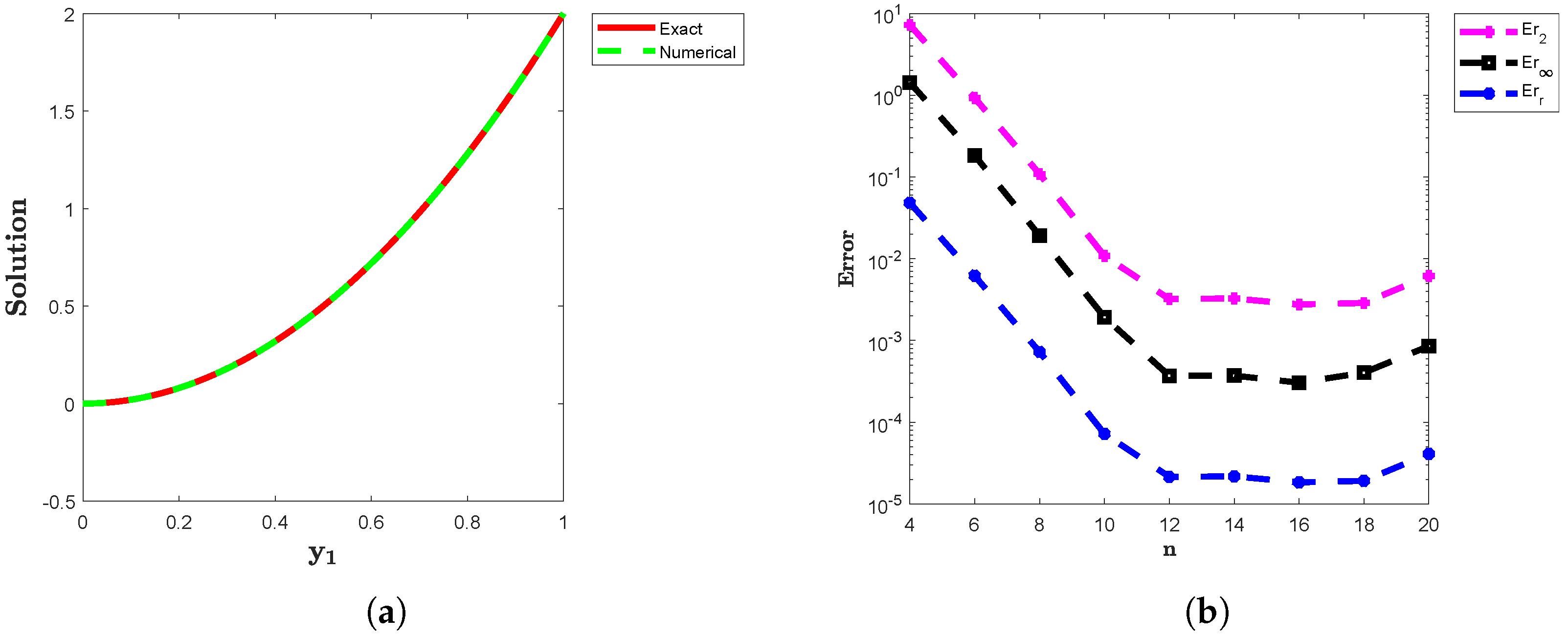
The exact solution for Example 1 is given by $Y(y_1,t)=y_1^2(t^{{\displaystyle \frac{5}{3}}}+t^{{\displaystyle \frac{4}{3}}}).$ Table 1 presents the error norms $E{r}_2$, $E{r}_{\infty },$ and $E{r}_r$ for various values of the parameters n, $N_l$, and $N_g$. In Figure 1a, we plot the approximate and exact solutions, while Figure 1b illustrates the comparison of $E{r}_2$, $E{r}_{\infty },$ and $E{r}_r$ as a function of n. The results demonstrate the convergence of our method as the parameter n increases, enhancing the accuracy in approximations. Moreover, we compared our results with two established methods: a spectral method and a numerical method using Müntz–Legendre polynomials. Our method’s results show a high level of agreement with these approaches, confirming the reliability and effectiveness of the proposed method in solving the problem accurately.

Table 1. Numerical results obtained using the proposed method.

	n	${\mathit{N}}_{\mathit{l}}$	${\mathit{N}}_{\mathit{g}}$	${\mathit{Er}}_2$	${\mathit{Er}}_{\mathit{\infty }}$	${\mathit{Er}}_{\mathit{r}}$	C.Time (s)
	10	5	150	1.0806 $\times {10}^{-2}$	1.9230 $\times {10}^{-3}$	8.8231 $\times {10}^{-4}$	0.23683
	12			3.2171 $\times {10}^{-3}$	3.6957 $\times {10}^{-4}$	2.6268 $\times {10}^{-4}$	0.23956
	14			3.2628 $\times {10}^{-3}$	3.7139 $\times {10}^{-4}$	2.6641 $\times {10}^{-4}$	0.23173
	16			2.7582 $\times {10}^{-3}$	3.0427 $\times {10}^{-4}$	2.2521 $\times {10}^{-4}$	0.27219
	20	5	140	5.7530 $\times {10}^{-3}$	8.3405 $\times {10}^{-4}$	4.8622 $\times {10}^{-4}$	0.19051
			145	5.6031 $\times {10}^{-3}$	8.0681 $\times {10}^{-4}$	4.6531 $\times {10}^{-4}$	0.22626
			150	6.1576 $\times {10}^{-3}$	8.5326 $\times {10}^{-4}$	5.0277 $\times {10}^{-4}$	0.18352
			155	5.8388 $\times {10}^{-3}$	8.1210 $\times {10}^{-4}$	4.6898 $\times {10}^{-4}$	0.23380
	20	5	140	5.7530 $\times {10}^{-3}$	8.3405 $\times {10}^{-4}$	4.8622 $\times {10}^{-4}$	0.19051
		6		5.1961 $\times {10}^{-3}$	7.6542 $\times {10}^{-4}$	4.3915 $\times {10}^{-4}$	0.18985
		7		5.7623 $\times {10}^{-3}$	8.3601 $\times {10}^{-4}$	4.8701 $\times {10}^{-4}$	0.16391
		8		5.6188 $\times {10}^{-3}$	8.1878 $\times {10}^{-4}$	4.7487 $\times {10}^{-4}$	0.16209
[19]					1.1907 $\times {10}^{-4}$
[24]					1.0408 $\times {10}^{-4}$

Figure 1. (a) The approximate and analytical solutions of Example 1 provide a comparative view of the method’s accuracy. (b) The plots of the error norms $E{r}_2$, $E{r}_{\infty },$ and $E{r}_r$ for Example 1.

• Example 2

We considered the FDPDE

$$D_t^{\alpha }Y(y_1,t)={\displaystyle \frac{{\partial }^{2}Y(y_1,t)}{\partial y_1^2}}-Y(y_1,t-1)+f(y_1,t).$$

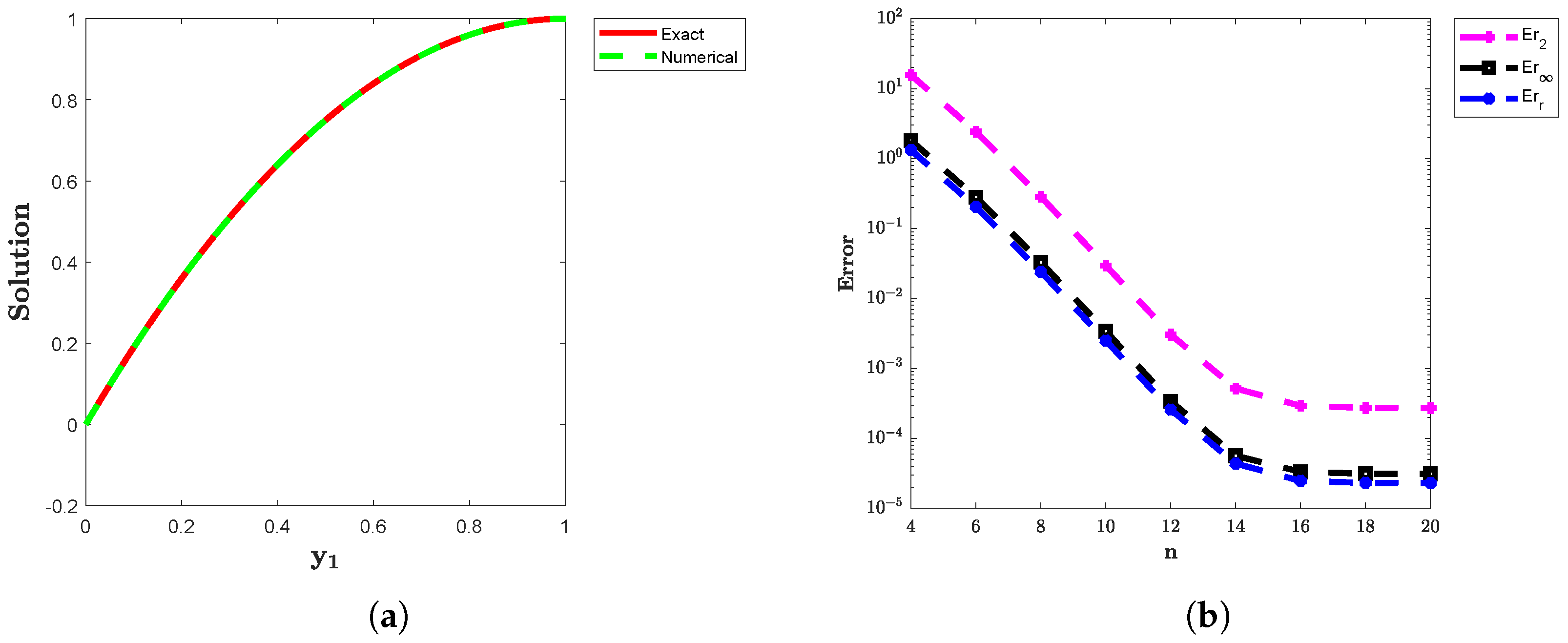
The analytical solution for Example 2 is given by $Y(y_1,t)=t^2(2y_1-y_1^2).$ Table 2 summarizes the error values $E{r}_2$, $E{r}_{\infty },$ and $E{r}_r$ for various parameters n, $N_l$, and $N_g$. Additionally, Table 2 shows that varying the quadrature nodes (n) and spatial nodes in both local and global domains $(N_l,N_g)$ consistently yields accurate and stable results. In Figure 2a, the approximate solution is plotted alongside the exact solution, offering a visual comparison, while Figure 2b provides a detailed look at the error measures $E{r}_2$, $E{r}_{\infty },$ and $E{r}_r$, which vary with increasing n. The results demonstrate a clear reduction in error as n grows, highlighting the improved accuracy of the method with higher n values.

Table 2. Numerical results obtained using the proposed method.

n	${\mathit{N}}_{\mathit{l}}$	${\mathit{N}}_{\mathit{g}}$	${\mathit{Er}}_2$	${\mathit{Er}}_{\mathit{\infty }}$	${\mathit{Er}}_{\mathit{r}}$	C.Time (s)
12	5	150	3.4520 $\times {10}^{-3}$	3.9102 $\times {10}^{-4}$	2.8185 $\times {10}^{-4}$	0.27943
14			8.2937 $\times {10}^{-4}$	9.7704 $\times {10}^{-5}$	6.7718 $\times {10}^{-5}$	0.15189
16			5.9220 $\times {10}^{-4}$	7.1160 $\times {10}^{-5}$	4.8353 $\times {10}^{-5}$	0.20869
18			5.7159 $\times {10}^{-4}$	6.8855 $\times {10}^{-5}$	4.6670 $\times {10}^{-5}$	0.23269
20	5	140	3.1465 $\times {10}^{-4}$	4.1967 $\times {10}^{-5}$	2.6592 $\times {10}^{-5}$	0.19989
		145	1.0719 $\times {10}^{-4}$	1.9084 $\times {10}^{-5}$	8.9020 $\times {10}^{-6}$	0.23217
		150	5.6985 $\times {10}^{-4}$	6.8661 $\times {10}^{-5}$	4.6528 $\times {10}^{-5}$	0.19689
		155	1.3517 $\times {10}^{-4}$	3.8157 $\times {10}^{-5}$	1.0857 $\times {10}^{-5}$	0.25788
20	5	140	3.1465 $\times {10}^{-4}$	4.1967 $\times {10}^{-5}$	2.6592 $\times {10}^{-5}$	0.15638
	6		7.8911 $\times {10}^{-4}$	9.0297 $\times {10}^{-5}$	6.6692 $\times {10}^{-5}$	0.17613
	7		4.1565 $\times {10}^{-4}$	4.4918 $\times {10}^{-5}$	3.5128 $\times {10}^{-5}$	0.17158
	8		2.7142 $\times {10}^{-4}$	3.1109 $\times {10}^{-5}$	2.2940 $\times {10}^{-5}$	0.20939

Figure 2. (a) The approximate and analytical solutions of Example 2 offer a clear comparison, highlighting the accuracy of the proposed method. (b) The plots of the error norms $E{r}_2$, $E{r}_{\infty },$ and $E{r}_r$ for Example 2.

• Example 3

We considered the FDPDE

$$D_t^{\alpha }Y(y_1,t)+D_t^{\alpha }Y(y_1,t-0.1)={\displaystyle \frac{1}{2}}{\displaystyle \frac{{\partial }^{2}Y(y_1,t)}{\partial y_1^2}}+{\displaystyle \frac{1}{2}}{\displaystyle \frac{{\partial }^{2}Y(y_1,t-0.1)}{\partial y_1^2}}+f(y_1,t).$$

The analytical solution for Example 3 is given by $Y(y_1,t)=t^{2}cos\left(\pi y_1\right).$ Table 3 provides error values $E{r}_2$, $E{r}_{\infty },$ and $E{r}_r$ corresponding to different values of parameters n, $N_l$, and $N_g$. In Figure 3a, the approximate and analytical solutions are plotted, while Figure 3b shows the comparison of errors $E{r}_2$, $E{r}_{\infty },$ and $E{r}_r$ versus n. These results demonstrate a consistent decrease in error as n grows, highlighting the improved accuracy of the method with higher values of $n.$

Table 3. Numerical results obtained using the proposed method.

n	${\mathit{N}}_{\mathit{l}}$	${\mathit{N}}_{\mathit{g}}$	${\mathit{Er}}_2$	${\mathit{Er}}_{\mathit{\infty }}$	${\mathit{Er}}_{\mathit{r}}$	C.Time (s)
10	5	150	2.9904 $\times {10}^{-2}$	3.4539 $\times {10}^{-3}$	2.4417 $\times {10}^{-3}$	0.213153
12			3.2903 $\times {10}^{-3}$	3.9096 $\times {10}^{-4}$	2.6865 $\times {10}^{-4}$	0.264186
14			7.4328 $\times {10}^{-4}$	9.7642 $\times {10}^{-5}$	6.0688 $\times {10}^{-5}$	0.268919
16			5.1361 $\times {10}^{-4}$	7.1098 $\times {10}^{-5}$	4.1936 $\times {10}^{-5}$	0.201902
20	5	140	2.8549 $\times {10}^{-4}$	4.1927 $\times {10}^{-5}$	2.4128 $\times {10}^{-5}$	0.248968
		145	8.1001 $\times {10}^{-5}$	1.9058 $\times {10}^{-5}$	6.7267 $\times {10}^{-6}$	0.220040
		150	4.9204 $\times {10}^{-4}$	6.8599 $\times {10}^{-5}$	4.0175 $\times {10}^{-5}$	0.218618
		155	2.4802 $\times {10}^{-4}$	3.8131 $\times {10}^{-5}$	1.9921 $\times {10}^{-5}$	0.225091
20	4	140	2.7496 $\times {10}^{-4}$	3.0935 $\times {10}^{-5}$	2.3238 $\times {10}^{-5}$	0.211381
	5		2.8549 $\times {10}^{-4}$	4.1927 $\times {10}^{-5}$	2.4128 $\times {10}^{-5}$	0.197186
	6		2.8003 $\times {10}^{-4}$	3.7854 $\times {10}^{-5}$	2.3667 $\times {10}^{-5}$	0.197116
	7		2.0725 $\times {10}^{-4}$	2.8481 $\times {10}^{-5}$	1.7516 $\times {10}^{-5}$	0.197540

Figure 3. The approximate and analytical solutions of Example 3 offer a distinct comparison, the close match between the two solutions showcases the method’s accuracy and robustness. (b) The plots of the error norms $E{r}_2$, $E{r}_{\infty },$ and $E{r}_r$ for Example 3.

• Example 4

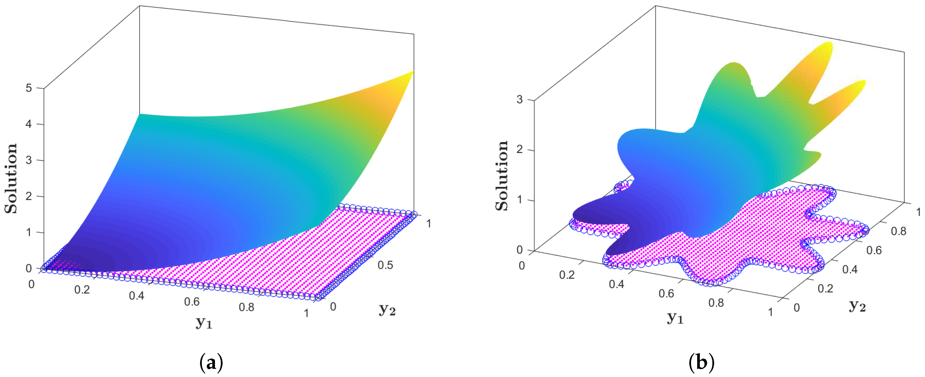
We considered the FDPDE

$$D_t^{\alpha }Y(y_1,y_2,t)={\displaystyle \frac{{\partial }^{2}Y(y_1,y_2,t)}{\partial y_1^2}}+{\displaystyle \frac{{\partial }^{2}Y(y_1,y_2,t)}{\partial y_2^2}}+Y(y_1,y_2,t-1)+f(y_1,y_2,t).$$

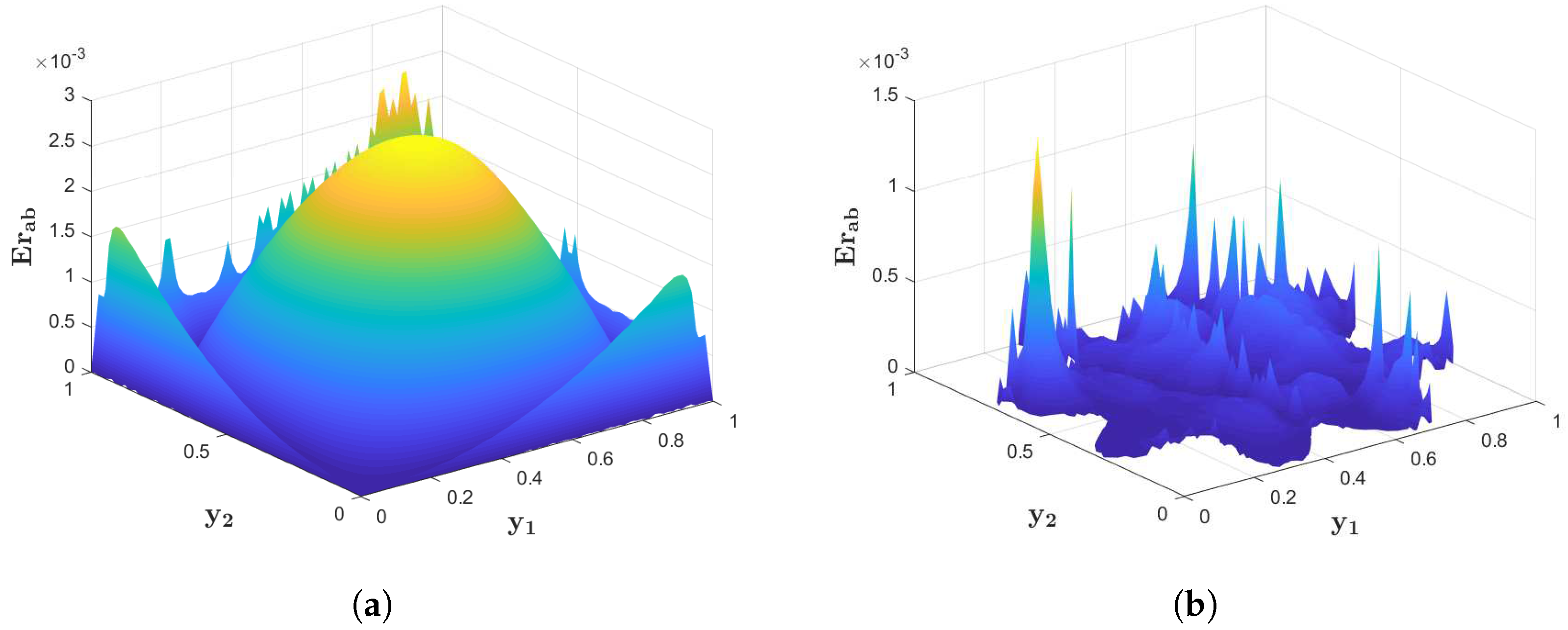
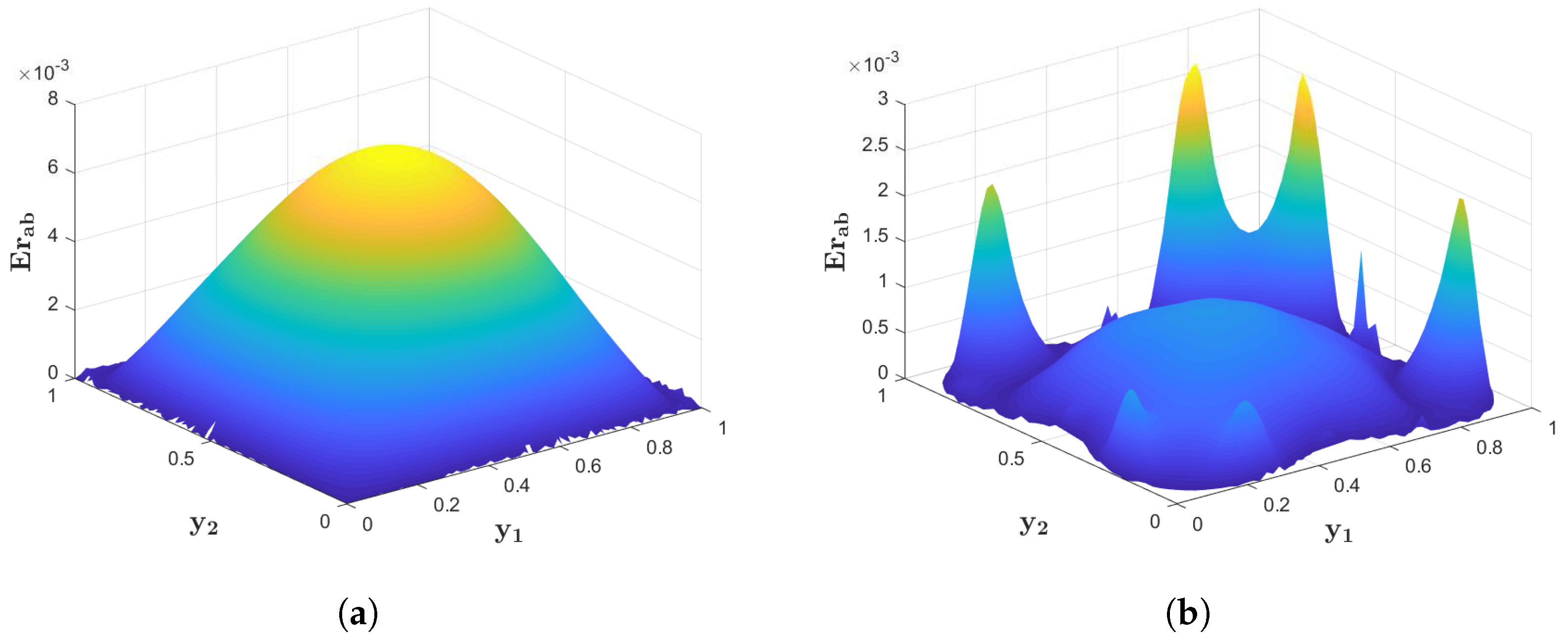
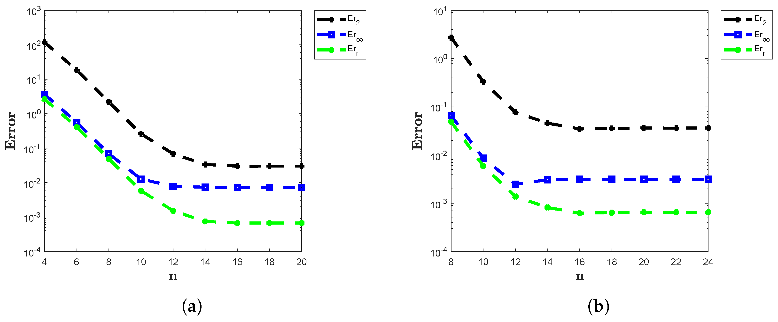
The exact solution for Example 4 is given as $Y(y_1,y_2,t)=(y_1^2+y_2^2)(t^{{\displaystyle \frac{5}{3}}}+t^{{\displaystyle \frac{4}{3}}}).$ Table 4 and Table 5 present the error norms $E{r}_2$, $E{r}_{\infty },$ and $E{r}_r$ for computation on square and star-shaped domains, respectively, using various values of n, $N_l$, and $N_g$. Figure 4a,b illustrate the numerical solutions on these domains, while Figure 5a,b provide plots of the absolute error $E{r}_{ab}$. Moreover, Figure 6a,b show the comparison of errors $E{r}_2$, $E{r}_{\infty },$ and $E{r}_r$ as a function of n on the square and star-shaped domains, respectively. The results demonstrate that errors consistently decrease as n increases, highlighting the effectiveness of the proposed method for solving such problems. This approach is both stable and efficient, offering accurate results with minimal computational cost. The method’s robustness in managing complex PDEs is demonstrated by its ability to maintain accuracy across different domains.

Table 4. Numerical results obtained using the proposed method on the square domain.

n	${\mathit{N}}_{\mathit{l}}$	${\mathit{N}}_{\mathit{g}}$	${\mathit{Er}}_2$	${\mathit{Er}}_{\mathit{\infty }}$	${\mathit{Er}}_{\mathit{r}}$	C.Time (s)
12	16	2025	3.3998 $\times {10}^{-02}$	7.6448 $\times {10}^{-03}$	7.5551 $\times {10}^{-04}$	6.24823
14			3.2019 $\times {10}^{-02}$	7.3868 $\times {10}^{-03}$	7.1154 $\times {10}^{-04}$	7.14549
16			6.5277 $\times {10}^{-02}$	1.7359 $\times {10}^{-02}$	1.6319 $\times {10}^{-03}$	4.49721
26	19	625	1.2347 $\times {10}^{-01}$	3.5720 $\times {10}^{-02}$	4.9389 $\times {10}^{-03}$	0.94834
		900	3.7476 $\times {10}^{-02}$	1.1739 $\times {10}^{-02}$	1.2492 $\times {10}^{-03}$	1.66831
		1225	2.7553 $\times {10}^{-02}$	6.9510 $\times {10}^{-03}$	7.8723 $\times {10}^{-04}$	3.47059
		1600	1.1526 $\times {10}^{-02}$	3.4463 $\times {10}^{-03}$	2.8815 $\times {10}^{-04}$	6.99581
		2025	8.8557 $\times {10}^{-03}$	2.6084 $\times {10}^{-03}$	1.9679 $\times {10}^{-04}$	12.62023
26	18	1225	1.7728 $\times {10}^{-02}$	5.3470 $\times {10}^{-03}$	5.0653 $\times {10}^{-04}$	3.24201
	19		2.7553 $\times {10}^{-02}$	6.9510 $\times {10}^{-03}$	7.8723 $\times {10}^{-04}$	3.30529
	20		4.5751 $\times {10}^{-03}$	7.9876 $\times {10}^{-04}$	1.3854 $\times {10}^{-04}$	3.36371
	21		4.8488 $\times {10}^{-03}$	2.3260 $\times {10}^{-03}$	1.3072 $\times {10}^{-04}$	3.38244

Table 5. Numerical results obtained using the proposed method on the star-shaped domain.

n	${\mathit{N}}_{\mathit{l}}$	${\mathit{N}}_{\mathit{g}}$	${\mathit{Er}}_2$	${\mathit{Er}}_{\mathit{\infty }}$	${\mathit{Er}}_{\mathit{r}}$	C.Time (s)
28	60	3532	6.8815 $\times {10}^{-2}$	1.4622 $\times {10}^{-2}$	1.1579 $\times {10}^{-3}$	39.0371
		3537	3.3214 $\times {10}^{-2}$	7.3353 $\times {10}^{-3}$	5.5847 $\times {10}^{-4}$	42.6241
		3644	2.2331 $\times {10}^{-2}$	6.0228 $\times {10}^{-3}$	3.6993 $\times {10}^{-4}$	50.1169
		4040	2.2694 $\times {10}^{-2}$	1.1366 $\times {10}^{-3}$	3.5704 $\times {10}^{-4}$	66.5245
10	50	4457	9.3718 $\times {10}^{-2}$	7.9441 $\times {10}^{-3}$	1.4038 $\times {10}^{-3}$	28.8898
12		4457	2.2756 $\times {10}^{-2}$	6.5871 $\times {10}^{-3}$	3.4087 $\times {10}^{-4}$	33.1369
14		4457	1.8559 $\times {10}^{-2}$	6.4666 $\times {10}^{-3}$	2.7799 $\times {10}^{-4}$	36.6103
16		4457	1.8273 $\times {10}^{-2}$	6.4564 $\times {10}^{-3}$	2.7371 $\times {10}^{-4}$	40.9781

Figure 4. (a) Approximate solution of Example 4 on square domain. (b) Approximate solution of Example 4 on star-shaped domain.

Figure 5. (a) $E{r}_{ab}$ of the proposed numerical method applied to Example 4 on a square domain with $N_g=6400,N_l=50$, and $n=28$. (b) $E{r}_{ab}$ of the proposed numerical method applied to Example 4 on a star-shaped domain with $N_g=3947,N_l=50$, and $n=28$.

Figure 6. (a) Error norms $E{r}_2$, $E{r}_{\infty },$ and $E{r}_r$ of the proposed numerical method applied to Example 4 on a square domain with $N_g=2500,N_l=30,$ and $\alpha =0.5.$ (b) Error norms $E{r}_2$, $E{r}_{\infty },$ and $E{r}_r$ of the proposed numerical method applied to Example 4 on a star-shaped domain with $N_g=3079,N_l=50,$ and $\alpha =0.5$.

• Example 5

We considered the FDPDE

$$D_t^{\alpha }Y(y_1,y_2,t)={\displaystyle \frac{{\partial }^{2}Y(y_1,y_2,t)}{\partial y_1^2}}+{\displaystyle \frac{{\partial }^{2}Y(y_1,y_2,t)}{\partial y_2^2}}-Y(y_1,y_2,t-1)+f(y_1,y_2,t).$$

The exact solution for Example 5 is given by $Y(y_1,y_2,t)=t^2(2(y_1+y_2)--(y_1^2+y_2^2)).$ Table 6 and Table 7 display the error matrices $E{r}_2$, $E{r}_{\infty },$ and $E{r}_r$ on square and nut-shaped domains, respectively, for various values of n, $N_l$, and $N_g$. As the number of spatial and quadrature nodes increases, the method’s accuracy correspondingly improves. Figure 7a,b illustrate the numerical solutions on square and nut-shaped domains, while Figure 8a,b depict the absolute error $E{r}_{ab}$ for these domains. Additionally, Figure 9a,b compare $E{r}_2$, $E{r}_{\infty },$ and $E{r}_r$ a function of n on the square and nut-shaped domains, respectively. The results confirm this method’s strong suitability for FDPDEs, with high accuracy and flexibility across various domains.

Table 6. Numerical results obtained using the proposed method on square domain.

n	${\mathit{N}}_{\mathit{l}}$	${\mathit{N}}_{\mathit{g}}$	${\mathit{Er}}_2$	${\mathit{Er}}_{\mathit{\infty }}$	${\mathit{Er}}_{\mathit{r}}$	C.Time (s)
12	16	2025	8.0728 $\times {10}^{-02}$	4.9320 $\times {10}^{-03}$	1.7940 $\times {10}^{-03}$	6.21129
14			3.8373 $\times {10}^{-02}$	4.4200 $\times {10}^{-03}$	8.5274 $\times {10}^{-04}$	7.18309
16			2.8381 $\times {10}^{-02}$	4.3738 $\times {10}^{-03}$	6.3069 $\times {10}^{-04}$	8.01589
18			2.7921 $\times {10}^{-02}$	4.3697 $\times {10}^{-03}$	6.2047 $\times {10}^{-04}$	9.08431
20			2.8580 $\times {10}^{-02}$	4.3694 $\times {10}^{-03}$	6.3512 $\times {10}^{-04}$	9.73357
26	19	625	7.9847 $\times {10}^{-02}$	2.0370 $\times {10}^{-02}$	3.1939 $\times {10}^{-03}$	0.95755
		900	2.4581 $\times {10}^{-02}$	6.4531 $\times {10}^{-03}$	8.1937 $\times {10}^{-04}$	1.74576
		1225	2.2435 $\times {10}^{-02}$	4.4067 $\times {10}^{-03}$	6.4099 $\times {10}^{-04}$	3.43286
		1600	1.0175 $\times {10}^{-02}$	1.9675 $\times {10}^{-03}$	2.5437 $\times {10}^{-04}$	6.918169
		2025	1.1537 $\times {10}^{-02}$	1.6446 $\times {10}^{-03}$	2.5637 $\times {10}^{-04}$	12.65923
26	18	1225	1.5194 $\times {10}^{-02}$	3.6216 $\times {10}^{-03}$	4.3411 $\times {10}^{-04}$	3.25149
	19		2.2435 $\times {10}^{-02}$	4.4067 $\times {10}^{-03}$	6.4099 $\times {10}^{-04}$	3.41734
	20		8.3794 $\times {10}^{-03}$	5.4477 $\times {10}^{-04}$	2.3941 $\times {10}^{-04}$	3.32513
	21		8.4121 $\times {10}^{-03}$	1.2926 $\times {10}^{-03}$	2.4035 $\times {10}^{-04}$	3.47378

Table 7. Numerical results obtained using the proposed method on the nut-shaped domain.

n	${\mathit{N}}_{\mathit{l}}$	${\mathit{N}}_{\mathit{g}}$	${\mathit{Er}}_2$	${\mathit{Er}}_{\mathit{\infty }}$	${\mathit{Er}}_{\mathit{r}}$	C.Time (s)
26	60	2637	6.5626 $\times {10}^{-2}$	2.2578 $\times {10}^{-2}$	1.2780 $\times {10}^{-3}$	23.9553
		3124	3.9210 $\times {10}^{-2}$	3.0689 $\times {10}^{-3}$	7.0153 $\times {10}^{-4}$	39.0850
		3134	3.6764 $\times {10}^{-2}$	3.0949 $\times {10}^{-3}$	6.5672 $\times {10}^{-4}$	33.7535
		3667	3.3639 $\times {10}^{-2}$	3.9441 $\times {10}^{-3}$	5.5551 $\times {10}^{-4}$	47.5117
24	65	3473	4.6859 $\times {10}^{-2}$	4.6491 $\times {10}^{-3}$	7.9514 $\times {10}^{-4}$	40.1300
26			4.6679 $\times {10}^{-2}$	4.6497 $\times {10}^{-3}$	7.9209 $\times {10}^{-4}$	45.3024
28			4.6047 $\times {10}^{-2}$	4.6570 $\times {10}^{-3}$	7.8136 $\times {10}^{-4}$	46.3791
30			4.4117 $\times {10}^{-2}$	4.6692 $\times {10}^{-3}$	7.4861 $\times {10}^{-4}$	49.5957

Figure 7. (a) Approximate solution of Example 5 on square domain. (b) Approximate solution of Example 5 on nut-shaped domain.

Figure 8. (a) $E{r}_{ab}$ of the proposed numerical method applied to Example 5 on a square domain with $N_g=7225,N_l=60$, and $n=26$. (b) $E{r}_{ab}$ of the proposed numerical method applied to Example 5 on a nut-shaped domain with $N_g=3697,N_l=55$, and $n=24$.

Figure 9. (a) Error norms $E{r}_2$, $E{r}_{\infty },$ and $E{r}_r$ of the proposed numerical method applied to Example 5 on a square domain with $N_g=2025,N_l=16,$ and $\alpha =0.5.$ (b) Error norms $E{r}_2$, $E{r}_{\infty },$ and $E{r}_r$ of the proposed numerical method applied to Example 5 on a nut-shaped domain with $N_g=3134,N_l=60,$ and $\alpha =0.5$.

7. Conclusions

A robust numerical method based on LT and local RBF methods for the solution of FDPDEs was successfully developed in this paper. This work demonstrates that the hybrid method not only solves the challenges posed by the FDPDEs but also provides an accurate and adaptable framework for obtaining solutions in both 1D and 2D domains. Furthermore, we employed the techniques from functional analysis to establish the existence and uniqueness of solutions to the considered problem. To demonstrate the efficiency of the proposed LT-based local RBF method, we solved three 1D problems and two 2D problems. The 2D problems were solved on both regular and irregular domains, with the first 2D problem solved on square and star-shaped domains, and the second 2D problem solved on square and nut-shaped domains. These examples highlight the adaptability and flexibility of the local RBF method coupled with the LT method for problems defined on irregular domains. In particular, the solutions obtained on star-shaped and nut-shaped domains demonstrate that our method can handle complex domains with acceptable accuracy. Additionally, we compared our 1D results with those of other methods, and the outcome shows close agreement, further validating the robustness of the proposed numerical method. As a future direction, we plan to extend this method to 3D problems, incorporating multiple delay terms to explore its effectiveness in more complex scenarios.