Article

Study on Abundant Dust-Ion-Acoustic Solitary Wave Solutions of a (3+1)-Dimensional Extended Zakharov–Kuznetsov Dynamical Model in a Magnetized Plasma and Its Linear Stability

1
Department of Mathematics and Statistics, Sub-CampusDepalpur, University of Agriculture Faisalabad, Faisalabad 38000, Pakistan
2
Department of Mathematics and Statistics, University of Agriculture Faisalabad, Faisalabad 38000, Pakistan
3
Mathematics Department, Faculty of Science, Taibah University, Al-Madinah Al-Munawarah 41411, Saudi Arabia
4
Department of Mathematics and Statistics, The University of Lahore, Lahore 54000, Pakistan
*
Author to whom correspondence should be addressed.
Fractal Fract. 2023, 7(9), 691; https://doi.org/10.3390/fractalfract7090691
Submission received: 12 August 2023 / Revised: 29 August 2023 / Accepted: 9 September 2023 / Published: 18 September 2023
(This article belongs to the Special Issue Spectral Methods for Fractional Functional Models)

Abstract

:
This article examines how shocks and three-dimensional nonlinear dust-ion-acoustic waves propagate across uniform magnetized electron–positron–ion plasmas. The two-variable  ( G / G , 1 / G ) -expansion and generalized exp( ϕ ( ξ ) )-expansion techniques are presented to construct the ion-acoustic wave results of a (3+1)-dimensional extended Zakharov–Kuznetsov (eZK) model. As a result, the novel soliton and other wave solutions in a variety of forms, including kink- and anti-kink-type breather waves, dark and bright solitons, kink solitons, and multi-peak solitons, etc., are attained. With the help of software, the solitary wave results (that signify the electrostatic potential field), electric and magnetic fields, and quantum statistical pressures are also constructed. These solutions have numerous applications in various areas of physics and other areas of applied sciences. Graphical representations of some of the obtained results, and the electric and magnetic fields as well as the electrostatic field potential are also presented. These results demonstrate the effectiveness of the presented techniques, which will also be useful in solving many other nonlinear models that arise in mathematical physics and several other applied sciences fields.

1. Introduction

Nonlinear partial differential equations (NLPDEs) describing nonlinear complex physical phenomena actively play a key role in many areas of applied sciences, particularly in plasma physics. In recent decades, it has become more important to locate exact solutions to nonlinear PDEs, due to the fact that nonlinear PDEs arise in many fields of engineering, mechanics, and physics [1,2,3,4]. We are able to recognize the mechanism behind these physical models by the study of exact solutions. To accomplish these aims, various efficient schemes have been established to identify the exact solutions of nonlinear PDEs, however, it is a difficult task. In plasma physics, nonlinear pulse propagation is defined by the ZK equation, which controls the characteristics of weakly nonlinear ion-acoustic waves in plasma made up of cold ions and hot, isothermal electrons in uniform magnetic fields [3,4]. There are several applications of the ZK equation in plasma physics, engineering, and applied sciences. Specifically, among the highly significant equations explored in the context of plasma physics is the ZK equation [5,6,7,8,9,10].
One of the most well-known and inspiring characteristics of nonlinear phenomena, particularly in extended models, which have many significant properties, is solitary waves. One of the two extensively researched canonical two-dimensional extensions of the KdV model is the ZK model [11]. The discussion of dust-ion-acoustic nonlinear waves in magnetized two-ion-temperature dusty plasmas, the proliferation of ion-acoustic waves with low frequencies in a bushy quantum magneto-plasma, etc., are discussed through nonlinear extended ZK equations [12,13,14]. Recently, using the theory of reductive perturbation, the researchers in [15] derived the three-dimensional eZK (3-deZK) model in a magnetized dusty plasma of two ion temperatures.
Several scholars have recently focused a lot of their effort on researching solitary wave results of NLPDEs [16,17,18], which transpire in applied sciences. Hence, several effective techniques have been established to create the solitary wave and soliton solutions, for instance, the inverse scattering scheme, direct algebraic approach [19], Backlund transform approach [20], Hirota’s bilinear technique [21], exp ( ϕ ( η ) ) -expansion techniques [22], extended tanh approach [23], auxiliary equation techniques [24], mapping techniques [25], rational expansion approach [26], elliptic function scheme [27], and numerous others [28]. Various numerical techniques have also been established, like the Adomian decomposition approach [29], homotopy analysis approach [30], homotopy perturbation approach [31], differential transform methods [32,33,34,35], etc., to achieve several forms of numerical solutions in nonlinear PDEs. The study of soliton solutions, structures, interactions, and other features has drawn a lot of interest, and it has successfully produced a number of significant findings [13,14,15,36].
The  ( G / G ) -expansion method was introduced in [37] for consistent study of exact solutions of NLPDEs. After that, an amended version, which is called the extended  ( G / G ) -expansion method, was constructed in [38]. Afterward, a generalized  ( G / G ) -expansion method was established [39]. Later, a two-variable  ( G / G , 1 / G ) -expansion technique was introduced in [40] and applied to nonlinear PDEs [41]. The  ( G / G , 1 / G ) -expansion method is believed to be a generalization of the  ( G / G ) -expansion approach. This attribute enables us to uncover new and more generic solutions. This viewpoint gave us inspiration to perform this study.
The overall structure of the remaining article can be outlined as follows: Section 2 elaborates on the proposed methods in detail. In Section 3, the given techniques are applied on the eZK equation to generate accurate wave results. The stability of the model is examined in Section 4. Section 5 analyzes the results and offers a physical justification. Section 6 summarizes the entirety of the work.

2. Proposed Methods

We describe the algorithms of the two-variable  ( G / G , 1 / G ) -expansion and generalized exp( ϕ ( ξ ) )-expansion techniques to obtain the exact wave solutions of nonlinear PDEs. Let us suppose a general PDE in x and t as
P w , w t , w x , 2 w t 2 , 2 w x 2 , = 0 .
The transformation  w ( x , t ) = w ( ξ )  with  ξ = α x ω t  is utilized to alter Equation (1) to an ODE as
P w , ω d w d ξ , α d w d ξ , ω 2 d 2 w d ξ 2 , α 2 d 2 w d ξ 2 , ω α d 2 w d ξ 2 , = 0 .

2.1. Two-Variable  ( G / G , 1 / G ) -Expansion Technique

To obtain wave results for the mentioned equations, this section provides a detailed description of the proposed technique. The approach commences with a second-order linear ordinary differential equation (ODE) as follows:
G ( ξ ) + μ G ( ξ ) = ν ,
via considering
ϕ = G G , ψ = 1 G ,
To ensure the accuracy of the computing, it is important to consider the derivatives of the variables  ϕ  and  ψ  as follows:
ϕ = ϕ 2 + ν ψ μ , ψ = ϕ ψ .
The general results of Equation (3) can be categorized into three distinct cases.
Case 1: If  μ < 0 , then
G ( ξ ) = A 1 sinh ξ μ + A 2 cosh ξ μ + ν μ ,
with
ψ 2 = μ μ 2 σ + ν 2 ( μ 2 ψ ν + ϕ 2 ) , where σ = A 1 2 A 2 2 .
Case 2: If  μ > 0 , then
G ( η ) = A 1 sin ξ μ + A 2 cos ξ μ + ν μ ,
with
ψ 2 = μ μ 2 σ + ν 2 ( μ 2 ψ ν + ϕ 2 ) , where σ = A 1 2 + A 2 2 .
Case 3: If  μ = 0 , then
G ( ξ ) = A 1 ξ + A 2 + ν 2 ξ 2 ,
with
ψ 2 = ϕ 2 2 ν ψ A 1 2 2 ν A 2 .
  A 1  and  A 2  are constants in the above cases.
Step 1: When examining the solution of Equation (2), it becomes apparent that it takes the form in both  ψ  and  ϕ  as follows:
w ( η ) = j = 0 M a j ϕ j + j = 1 M b j ϕ j 1 ψ ,
here G correspond to (3). The coefficients  a j , b j , ω , α , and  ν  are constants. M can be established via utilizing the harmonizing principle on Equation (2).
Step 2: Upon substituting Equation (12) into (2), and considering Equations (5) and (7), a polynomial equation in terms of  ψ  and  ϕ  is derived, leading to the establishment of a system of algebraic equations.
Step 3: The system is resolved via using a software program. The wave solutions in Equation (2) are constructed as three different types of functions via exploiting the values of  a j b j , a μ ν A 1 , and  A 2 .
Step 4: The resolution procedure concludes by generating outcomes in Equation (1) through the utilization of the wave transformation  ξ = α x ω t  in a reverse manner.

2.2. Generalized Exp( ϕ ( ξ ) )-Expansion Scheme

To achieve exact solutions using this approach, it is essential to follow a specific set of steps:
Step 1: By considering Equation (2), which is obtained from Equation (1) using wave transformation,  ξ = α x ω t  assumes the following traveling wave solutions
w ( ξ ) = i = 0 M a i ( exp ( ϕ ( ξ ) ) ) i , a M 0 ,
including  ω ( x , t ) = ω ( ξ )  and satisfies the nonlinear ODE below.
ϕ ( ξ ) = μ exp ( ϕ ( ξ ) ) + ν exp ( ϕ ( ξ ) ) + λ ,
where the coefficients  a i , μ , ν , and  λ  are constants. M can be established via utilizing the harmonizing principle on Equation (2).
Step 2: The value of the positive integer M is subsequently determined by balancing the higher-order nonlinear term and higher-order derivative term of (12). The following formula is the detailed expression, assuming  D [ u ( ξ ) ] = n :
D d N v ( ξ ) d ξ N = N + ρ .
D v N d K v ( ξ ) d ξ K S = ρ N + S ( ρ + K ) .
Step 3: Substituting Equations (13) and (14) into Equation (2), yields a polynomial function of  e i ϕ ( ξ ) ; the parameters  a i ( 1 i N ) , k , ν , μ , λ , ω , and  α  can be determined.
Step 4: The resolution procedure concludes by generating outcomes in Equation (1) through the utilization of the wave transformation  ξ = α x ω t  in a reverse manner.

3. Formation of Soliton Solutions of (3+1)-Dimensional Extended Zakharov–Kuznetsov Dynamical Model

The (3+1)-dimensional extended ZK equation [3] can be written as
u t + k 1 u u x + k 2 u x x x + k 3 u x y y + u x z z = 0 .
Adopting the transformation as
U ( ξ ) = u ( x , y , z , t ) , ξ = α 1 x + α 2 y + α 3 z + ω t + ξ 0 ,
where  α 1 , α 2 , α 3 , and  ω  are the wave number and frequency of the solitons. Using Equation (18) in Equation (17) and the ODEs obtained gives
ω U + k 1 α 1 U U + k 2 α 1 3 + k 3 α 1 ( α 2 2 + α 3 2 ) U = 0 .
Integrating the above equation with respect to  η  yields
2 k 2 α 1 3 + k 3 α 1 ( α 2 2 + α 3 2 ) U + 2 ω U + k 1 α 1 U 2 = 0 .

3.1. Two-Variable  ( G / G , 1 / G ) -Expansion Technique

In this subpart, we construct the soliton wave solutions of the dynamical model (17) by using the two-variable  ( G / G , 1 / G ) -expansion technique. We use the balancing principle on Equation (20) and considering the solution as
U ( ξ ) = a 0 + a 1 ϕ ( ξ ) + a 2 ϕ ( ξ ) 2 + b 1 ψ ( ξ ) + b 2 ψ ( ξ ) ϕ ( ξ ) .
By utilizing Equation (21) alongside Equation (5) and incorporating them into (20), a system of equations in the variables  a 0 , a 1 , a 2 , b 1 , b 2 , α 1 , α 2 , α 3 , ν , ω ,  and  μ  is derived. This system is constructed by equating the coefficients of terms involving  ϕ i ψ j  to zero. Upon solving this system, the following results are obtained:
a 0 = 4 μ α 1 2 k 2 + α 2 2 k 3 + α 3 2 k 3 k 1 , a 2 = 12 α 1 2 k 2 + α 2 2 k 3 + α 3 2 k 3 k 1 , a 1 = b 1 = b 2 = ν = 0 , ω = 4 α 1 μ α 1 2 k 2 + α 2 2 k 3 + α 3 2 k 3 .
a 0 = 12 μ α 1 2 k 2 + α 2 2 k 3 + α 3 2 k 3 k 1 , a 2 = 12 α 1 2 k 2 + α 2 2 k 3 + α 3 2 k 3 k 1 , a 1 = b 1 = b 2 = ν = 0 , ω = 4 α 1 μ α 1 2 k 2 + α 2 2 k 3 + α 3 2 k 3 .
a 0 = a 2 μ 3 , a 1 = b 1 = b 2 = 0 , ν = 0 , ω = 4 α 1 μ α 1 2 k 2 + α 2 2 k 3 + α 3 2 k 3 , k 1 = 12 α 1 2 k 2 + α 2 2 k 3 + α 3 2 k 3 a 2 .
a 0 = a 2 μ , a 1 = b 1 = b 2 = ν = 0 , ω = 4 α 1 μ α 1 2 k 2 + α 2 2 k 3 + α 3 2 k 3 , k 1 = 12 α 1 2 k 2 + α 2 2 k 3 + α 3 2 k 3 a 2 .
From (22)–(24) the following results can be obtained.
Case I:  μ < 0  (hyperbolic function solution),
u 1 ( x , y , z , t ) = 4 μ α 1 2 k 2 + α 2 2 + α 3 2 k 3 2 A 2 A 1 sinh 2 μ ξ + A 1 2 cosh 2 μ ξ + 2 + A 2 2 cosh 2 μ ξ 2 k 1 A 1 sinh μ ξ + A 2 cosh μ ξ 2 .
u 2 ( x , y , z , t ) = 12 A 1 2 A 2 2 μ α 1 2 k 2 + α 2 2 + α 3 2 k 3 k 1 A 1 sinh μ ξ + A 2 cosh μ ξ 2 .
u 3 ( x , y , z , t ) = a 2 3 μ 3 μ A 2 sinh μ ξ + A 1 cosh μ ξ 2 A 1 sinh μ ξ + A 2 cosh μ ξ 2 .
Case II:  μ > 0  (trigonometric function solution),
u 4 ( x , y , z , t ) = 4 μ α 1 2 k 2 + α 2 2 + α 3 2 k 3 4 A 2 A 1 sinh 2 μ ξ + A 1 2 2 cosh 2 μ ξ + 1 + A 2 2 2 cosh 2 μ ξ 1 k 1 A 1 sinh μ ξ + A 2 cosh μ ξ 2 .
u 5 ( x , y , z , t ) = 12 μ α 1 2 k 2 + α 2 2 + α 3 2 k 3 2 A 2 A 1 sinh 2 μ ξ + A 1 2 cosh 2 μ ξ + A 2 2 cosh 2 μ ξ k 1 A 1 sinh μ ξ + A 2 cosh μ ξ 2 .
u 6 ( x , y , z , t ) = a 2 3 3 μ A 2 sinh μ ξ + A 1 cosh μ ξ 2 A 1 sinh μ ξ + A 2 cosh μ ξ 2 + μ .
Case III:  μ = 0  (rational function solution),
u 7 ( x , y , z , t ) = 4 μ ξ 2 + 3 α 1 2 k 2 + α 2 2 + α 3 2 k 3 k 1 ξ 2 .
u 8 ( x , y , z , t ) = 12 α 1 2 k 2 + α 2 2 + α 3 2 k 3 μ ξ 2 + 1 k 1 ξ 2 .
u 9 ( x , y , z , t ) = a 2 3 μ + 3 ξ 2 .
The motiosn and positions of the positrons and electrons as they transfer along their orbits in a uniformly magnetized electron–positron plasma define the electric and magnetic fields. The gradient of the scalar function  u 1 , often known as the electrostatic potential, is the electric field. The electric field “E” points from areas with high to low electric potential. The electric field is represented mathematically as
E = u = u x x ^ u y y ^ u z z ^ .
The electric fields of the electric potential,  u 1 u 2 , and  u 3 , are expressed as
E 1 = 24 A 1 2 A 2 2 ( μ ) 3 / 2 α 1 2 k 2 + α 2 2 + α 3 2 k 3 A 2 sinh μ ξ + A 1 cosh μ ξ k 1 A 1 sinh μ ξ + A 2 cosh μ ξ 3 · α 1 x ^ + α 2 y ^ + α 3 z ^ .
E 2 = 24 A 1 2 A 2 2 μ μ α 1 2 k 2 + α 2 2 + α 3 2 k 3 A 2 sinh μ ξ + A 1 cosh μ ξ k 1 A 1 sinh μ ξ + A 2 cosh μ ξ 3 · α 1 x ^ + α 2 y ^ + α 3 z ^ .
E 3 = 2 a 2 A 1 2 A 2 2 ( μ ) 3 / 2 A 2 sinh μ ξ + A 1 cosh μ ξ A 1 sinh μ ξ + A 2 cosh μ ξ 3 · α 1 x ^ + α 2 y ^ + α 3 z ^ .
E 4 = 24 A 1 2 A 2 2 μ 3 / 2 α 1 2 k 2 + α 2 2 + α 3 2 k 3 A 2 sinh μ ξ + A 1 cosh μ ξ k 1 A 1 sinh μ ξ + A 2 cosh μ ξ 3 · α 1 x ^ + α 2 y ^ + α 3 z ^ .
The Maxwell–Faraday equation provides the relationship between electric and magnetic fields as
× E = B t .
Utilizing the Maxwell–Faraday Equation (40), the magnetic field is constructed as
B 1 = 24 α 1 α 3 A 1 2 A 2 2 ( μ ) 3 / 2 α 1 2 k 2 + α 2 2 + α 3 2 k 3 A 2 sinh μ ξ + A 1 cosh μ ξ k 1 ω A 1 sinh μ ξ + A 2 cosh μ ξ 3 · α 2 x ^ + α 1 + α 3 y ^ α 2 z ^ .
B 2 = 24 A 1 2 A 2 2 ( μ ) 3 / 2 α 1 α 3 α 1 2 k 2 + α 2 2 + α 3 2 k 3 A 2 sinh μ ξ + A 1 cosh μ ξ k 1 ω A 1 sinh μ ξ + A 2 cosh μ ξ 3 · α 2 x ^ + α 1 + α 3 y ^ α 2 z ^ .
B 3 = 2 a 2 α 1 α 3 A 1 2 A 2 2 ( μ ) 3 / 2 A 2 sinh μ ξ + A 1 cosh μ ξ ω A 1 sinh μ ξ + A 2 cosh μ ξ 3 · α 2 x ^ α 1 + α 3 y ^ + α 2 z ^ .
B 4 = 24 α 1 α 3 A 1 2 A 2 2 μ 3 / 2 α 1 2 k 2 + α 2 2 + α 3 2 k 3 A 2 sinh μ ξ + A 1 cosh μ ξ k 1 ω A 1 sinh μ ξ + A 2 cosh μ ξ 3 · α 2 x ^ + α 1 + α 3 y ^ α 2 z ^ .
The electric number density, denoted by  n e , is used to describe the pressure of the electron fluid as  P = P ( n e ) . The following is the relationship between the electric number density  n e  and the electron fluid pressure P:
P = ν F e 2 m e 3 n 0 2 e 3 n e ,
where  ν F e 2  stands for the Fermi velocity of electrons, an electron’s mass is  m e , and  n 0  is the equilibrium density for both electrons and ions. This equation yields the electron’s quantum statistical pressure as
P 1 = ν F e 2 m e 3 n 0 2 Exp 12 μ α 1 2 k 2 + α 2 2 + α 3 2 k 3 2 A 2 A 1 sinh 2 μ ξ + A 1 2 cosh 2 μ ξ + 2 + A 2 2 cosh 2 μ ξ 2 k 1 A 1 sinh μ ξ + A 2 cosh μ ξ 2 .
P 2 = ν F e 2 m e 3 n 0 2 Exp 12 A 1 2 A 2 2 μ α 1 2 k 2 + α 2 2 + α 3 2 k 3 k 1 A 1 sinh μ ξ + A 2 cosh μ ξ 2 .
P 3 = ν F e 2 m e 3 n 0 2 Exp a 2 μ 3 μ A 2 sinh μ ξ + A 1 cosh μ ξ 2 A 1 sinh μ ξ + A 2 cosh μ ξ 2 .
P 4 = ν F e 2 m e 3 n 0 2 Exp 12 μ α 1 2 k 2 + α 2 2 + α 3 2 k 3 4 A 2 A 1 sinh 2 μ ξ + A 1 2 2 cosh 2 μ ξ + 1 + A 2 2 2 cosh 2 μ ξ 1 k 1 A 1 sinh μ ξ + A 2 cosh μ ξ 2 .
Similarly, the solutions of set (25) can be constructed in the more generalized form of a dynamical model (17).

3.2. Generalized Exp( ϕ ( ξ ) )-Expansion Method

In this part, we construct the wave results of the dynamical model (17) by using the generalized exp( ϕ ( ξ ) )-expansion technique. Using the balancing principle on Equation (20) and considering the solution as
U ( ξ ) = a 0 + a 1 e ϕ ( ξ ) + a 2 e 2 ϕ ( ξ ) .
By utilizing Equation (50) alongside Equation (5) and incorporating them into (20), a system of equations in variables  a 0 , a 1 , a 2 , k 1 , k 2 , k 3 , α 1 , α 2 , α 3 , ν , ω ,  and  μ  is derived. This system is constructed by equating the coefficients of terms involving  ϕ i  to zero. Upon solving this system, the following results are obtained:
a 1 = 12 λ μ α 1 2 k 2 + α 2 2 + α 3 2 k 3 k 1 , a 2 = 12 μ 2 α 1 2 k 2 + α 2 2 + α 3 2 k 3 k 1 , ϵ = α 1 a 0 k 1 + 12 μ ν α 1 2 k 2 + α 2 2 + α 3 2 k 3 a 0 k 1 + 2 α 1 2 k 2 + α 2 2 + α 3 2 k 3 λ 2 + 2 μ ν 2 k 1 , ω = α 1 a 0 k 1 + α 1 2 k 2 + α 2 2 + α 3 2 k 3 λ 2 + 8 μ ν .
a 0 = 12 μ ν α 1 2 k 2 + α 2 2 + α 3 2 k 3 k 1 , a 1 = 12 λ μ α 1 2 k 2 + α 2 2 + α 3 2 k 3 k 1 , a 2 = 12 μ 2 α 1 2 k 2 + α 2 2 + α 3 2 k 3 k 1 , ϵ = 0 , ω = ± α 1 α 1 2 k 2 + α 2 2 + α 3 2 k 3 λ 2 4 μ ν .
a 2 = a 1 μ λ , α 3 = ± a 1 k 1 12 λ μ α 1 2 k 2 + α 2 2 k 3 2 3 λ k 3 μ , ω = α 1 k 1 a 1 λ 2 + 8 μ ν 12 a 0 λ μ 12 λ μ , ϵ = α 1 k 1 a 0 λ a 1 ν a 1 λ 2 + 2 μ ν 6 a 0 λ μ 12 λ 2 μ .
The following results, in the form of solitons and other waves from set (51), can be obtained as
Family 1: For  μ = 1 ,
u 1 ( x , y , z , t ) = a 0 + 24 ν α 1 2 k 2 + α 2 2 + α 3 2 k 3 λ λ 2 4 ν tanh λ 2 4 ν 2 ξ + ξ 0 + λ 2 2 ν k 1 λ 2 4 ν tanh λ 2 4 ν 2 x ξ + ξ 0 λ 2 4 ν + λ 2 , ν 0 , λ 2 4 ν > 0 .
The electric and magnetic fields of  u 1  are expressed as
E 1 = 12 ν α 1 2 k 2 + α 2 2 + α 3 2 k 3 λ 2 4 ν 3 2 λ tanh λ 2 4 ν 2 ξ + ξ 0 + λ 2 4 ν sec h 2 λ 2 4 ν 2 ξ + ξ 0 k 1 λ 2 4 ν tanh λ 2 4 ν 2 ξ + ξ 0 + λ 3 · α 1 x ^ + α 2 y ^ + α 3 z ^ .
B 1 = 12 α 1 α 3 ν α 1 2 k 2 + α 2 2 + α 3 2 k 3 λ 2 4 ν 3 2 ν λ 2 2 ν sinh 2 λ 2 4 ν ξ + ξ 0 λ ν λ 2 4 ν cosh 2 λ 2 4 ν ξ + ξ 0 + λ λ 2 2 ν λ 2 4 ν cosh λ 2 4 ν ξ + ξ 0 + 3 λ ν λ 2 4 ν + 4 λ 2 ν λ 4 + 4 ν 2 sinh λ 2 4 ν ξ + ξ 0 / k 1 ω λ 2 2 ν + 2 ν cosh ξ + ξ 0 λ 2 4 ν 3 · α 2 x ^ α 1 + α 3 y ^ + α 2 z ^ .
The electron’s quantum statistical pressure is constructed as
P 1 = ν F e 2 m e 3 n 0 2 Exp 3 a 0 + 72 ν α 1 2 k 2 + α 2 2 + α 3 2 k 3 λ λ 2 4 ν tanh λ 2 4 ν 2 ξ + ξ 0 + λ 2 2 ν k 1 λ 2 4 ν tanh λ 2 4 ν 2 x ξ + ξ 0 λ 2 4 ν + λ 2 .
u 2 ( x , y , z , t ) = a 0 + 24 ν α 1 2 k 2 + α 2 2 + α 3 2 k 3 λ 2 2 ν λ 4 ν λ 2 tan 4 ν λ 2 2 ξ + ξ 0 k 1 λ 4 ν λ 2 tan 4 ν λ 2 2 ξ + ξ 0 2 , ν 0 , λ 2 4 ν < 0 .
The electric and magnetic fields of  u 2  are expressed as
E 2 = 12 ν α 1 2 k 2 + α 2 2 + α 3 2 k 3 λ 2 4 ν λ 2 4 ν λ 4 ν λ 2 tan 4 ν λ 2 2 ξ + ξ 0 sec 2 4 ν λ 2 2 ξ + ξ 0 k 1 λ 4 ν λ 2 tan 4 ν λ 2 2 ξ + ξ 0 3 · α 1 x ^ + α 2 y ^ + α 3 z ^ .
B 2 = 12 α 1 α 3 ν α 1 2 k 2 + α 2 2 + α 3 2 k 3 4 ν λ 2 3 2 ν 2 ν λ 2 sin 2 4 ν λ 2 ξ + ξ 0 + λ ν 4 ν λ 2 cos 2 4 ν λ 2 ξ + ξ 0 λ λ 2 2 ν 4 ν λ 2 cos 4 ν λ 2 ξ + ξ 0 3 λ ν 4 ν λ 2 + λ 4 4 λ 2 ν 4 ν 2 sin 4 ν λ 2 ξ + ξ 0 / k 1 ω λ 2 2 ν + 2 ν cos 4 ν λ 2 ξ + ξ 0 3 · α 2 x ^ + α 1 + α 3 y ^ α 2 z ^ .
The electron’s quantum statistical pressure is constructed as
P 2 = ν F e 2 m e 3 n 0 2 Exp a 0 + 72 ν α 1 2 k 2 + α 2 2 + α 3 2 k 3 λ 2 2 ν λ 4 ν λ 2 tan 4 ν λ 2 2 ξ + ξ 0 k 1 λ 4 ν λ 2 tan 4 ν λ 2 2 ξ + ξ 0 2 .
u 3 ( x , y , z , t ) = a 0 k 1 e λ ξ + ξ 0 1 2 12 λ 2 α 1 2 k 2 + α 2 2 + α 3 2 k 3 e λ ξ + ξ 0 k 1 e λ ξ + ξ 0 1 2 , ν = 0 , λ 0 , λ 2 4 ν > 0 .
u 4 ( x , y , z , t ) = a 0 + 3 λ 3 ξ + ξ 0 α 1 2 k 2 + α 2 2 + α 3 2 k 3 λ ξ + λ ξ 0 + 2 k 1 λ ξ + λ ξ 0 + 1 2 , ν 0 , λ 0 , λ 2 4 ν = 0 .
Family 2: For  λ = 0 ,
u 5 ( x , y , z , t ) = a 0 12 μ ν α 1 2 k 2 + α 2 2 + α 3 2 k 3 cot 2 μ ν ξ + ξ 0 k 1 , μ > 0 , ν > 0 .
The electric and magnetic fields of  u 5  are expressed as
E 5 = 24 α 1 2 k 2 + α 2 2 + α 3 2 k 3 ( μ ν ) 3 2 cot μ ν ξ + ξ 0 csc 2 μ ν ξ + ξ 0 k 1 · α 1 x ^ + α 2 y ^ + α 3 z ^ .
B 5 = 24 α 3 α 1 α 1 2 k 2 + α 2 2 + α 3 2 k 3 ( μ ν ) 3 2 cot μ ν ξ + ξ 0 csc 2 μ ν ξ + ξ 0 k 1 ω · α 2 x ^ α 1 + α 3 y ^ + α 2 z ^ .
The electron’s quantum statistical pressure is constructed as
P 5 = ν F e 2 m e 3 n 0 2 Exp 3 a 0 32 μ ν α 1 2 k 2 + α 2 2 + α 3 2 k 3 cot 2 μ ν ξ + ξ 0 k 1 .
u 6 ( x , y , z , t ) = a 0 12 μ ν α 1 2 k 2 + α 2 2 + α 3 2 k 3 cot 2 ξ ξ 0 μ ν k 1 , μ < 0 , ν < 0 .
u 7 ( x , y , z , t ) = a 0 + 12 μ ν α 1 2 k 2 + α 2 2 + α 3 2 k 3 coth 2 μ ν ξ ξ 0 k 1 , μ > 0 , μ < 0 .
u 8 ( x , y , z , t ) = a 0 + 12 μ ν α 1 2 k 2 + α 2 2 + α 3 2 k 3 coth 2 μ ν ξ + ξ 0 k 1 , μ < 0 , μ > 0 .
Family 3: For  ν = λ = 0 ,
u 9 ( x , y , z , t ) = a 0 12 α 1 2 k 2 + α 2 2 + α 3 2 k 3 k 1 ξ + ξ 0 2 .

4. Stability Analysis

Now, using a conventional linear stability analysis [], we look at the modulational instability of model (17). For model (17), the steady-state solution takes the following form:
u ( x , y , z , t ) = P + Φ ( x , y , z , t ) e ϕ ( t ) , ϕ ( t ) = β ϵ P t ,
where P is the normalized optical power. In order for  Φ < < P , perturbation  Φ ( x , y , z , t )  is introduced. By linearizing and substituting Equation (72) into Equation (17), we obtain
Φ t + k 2 3 Φ x 3 + k 3 x 2 Φ y 2 + 2 Φ z 2 + k 1 P Φ x + β P ϵ Φ = 0 .
considering the solution of Equation (73) takes
Φ ( x , y , z , t ) = ρ e δ 1 x + δ 2 y + δ 3 z ν t ,
where  δ 1 , δ 2 , δ 3 , and  ν  are the wave numbers and normalized frequency of  Φ ( x , y , z , t ) , respectively. When Equation (74) is substituted into Equation (73), the relation is as follows:
ν = δ 1 3 k 2 + k 3 δ 1 δ 2 2 + δ 3 2 + δ 1 k 1 P + β P ϵ .
The dispersion relation in Equation (75) shows that the wave number, modulation of self-phase, and stimulating Raman scattering have an impact on the steady-state stability. For all wave numbers  δ 1 , δ 2 , and  δ 3 , the  ν  in Equation (75) real and the steady-state is stable alongside small perturbations.

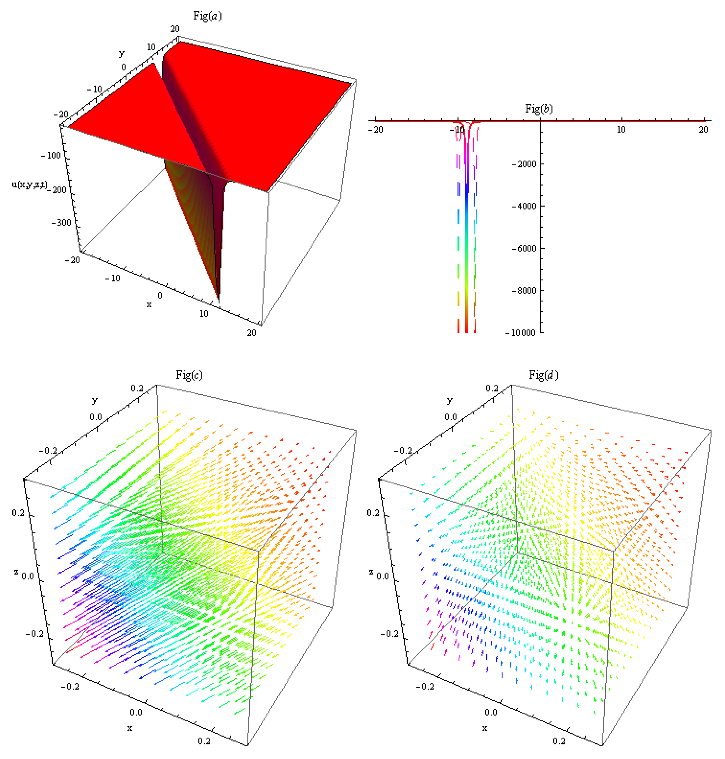
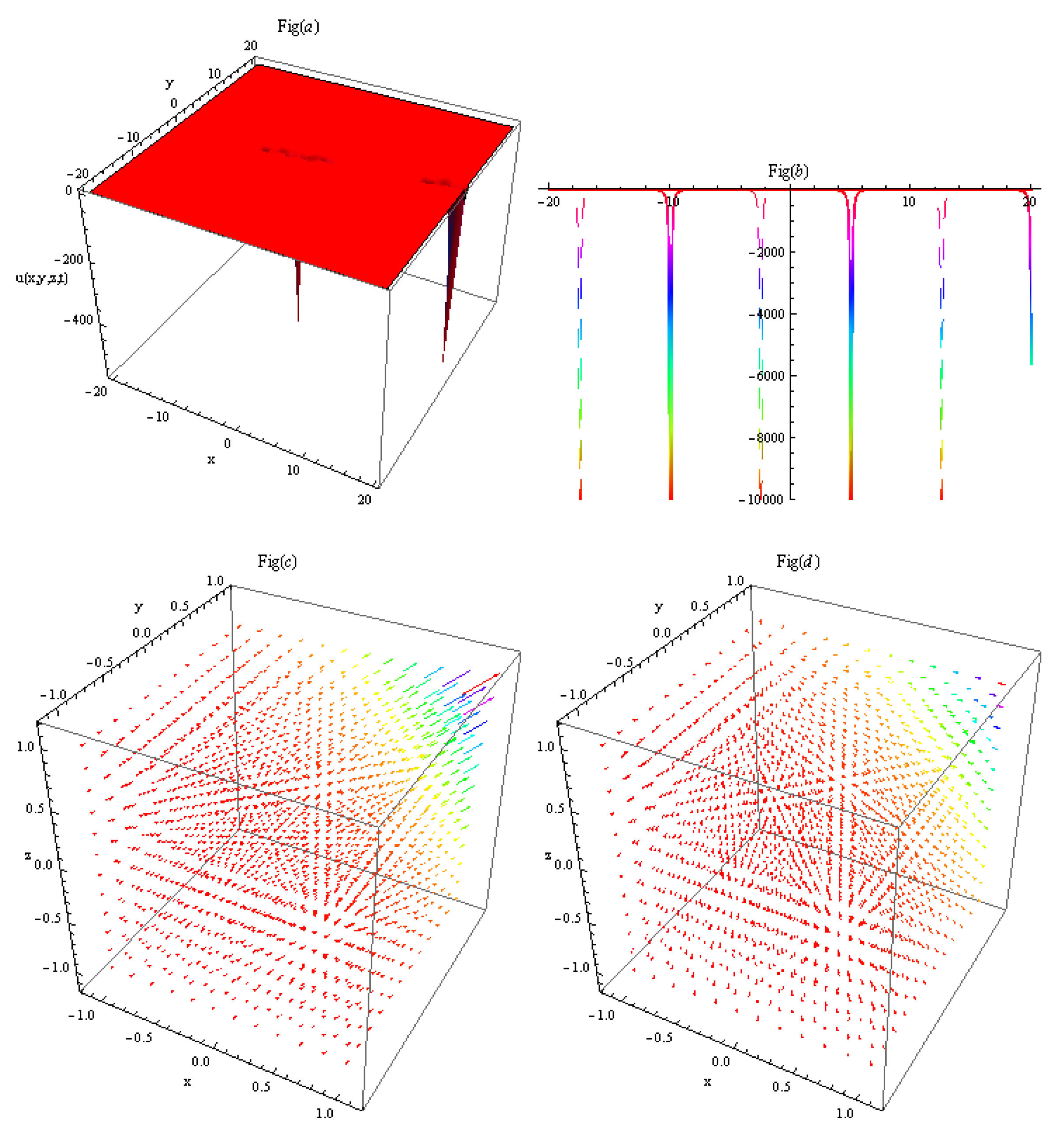
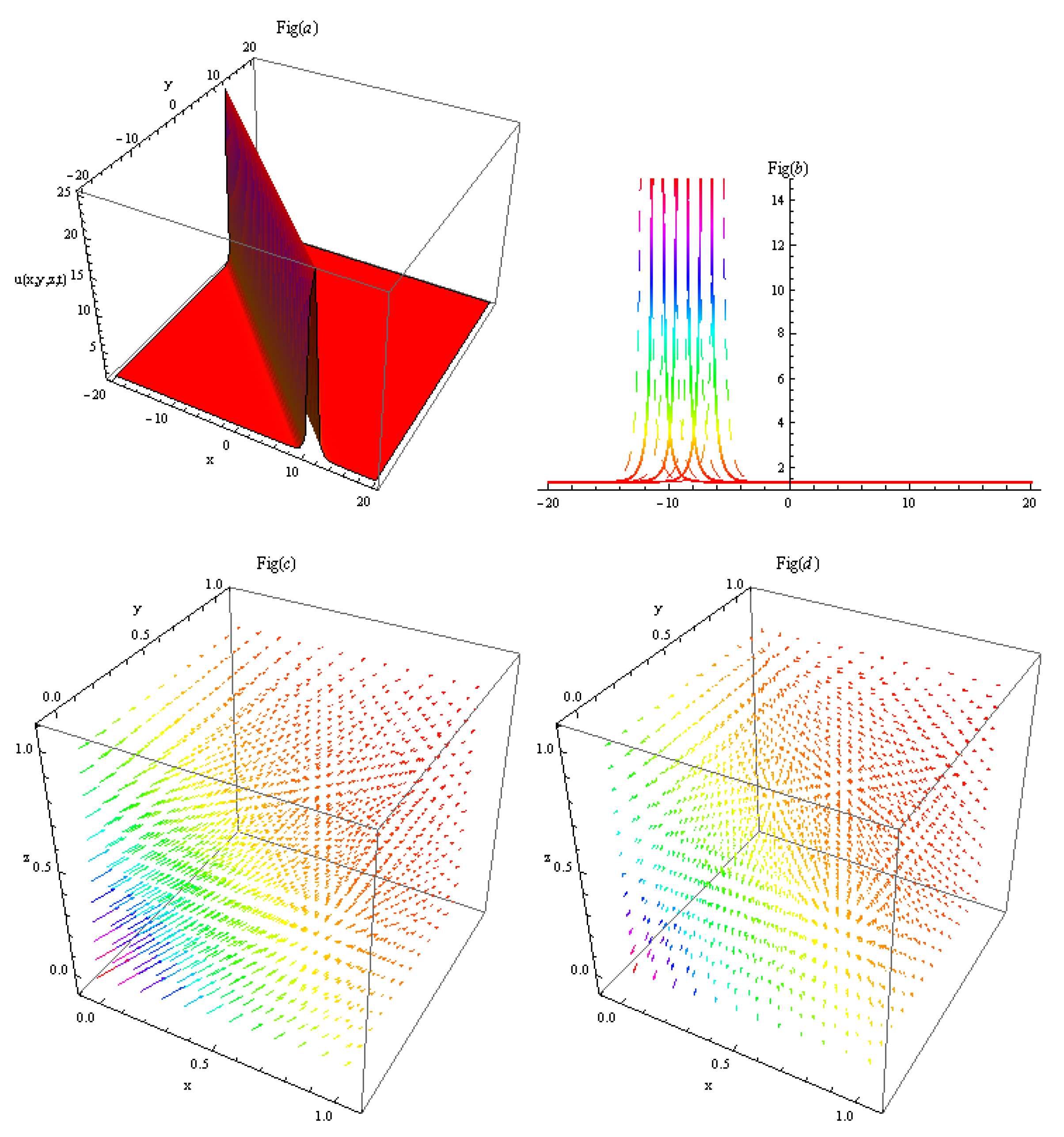
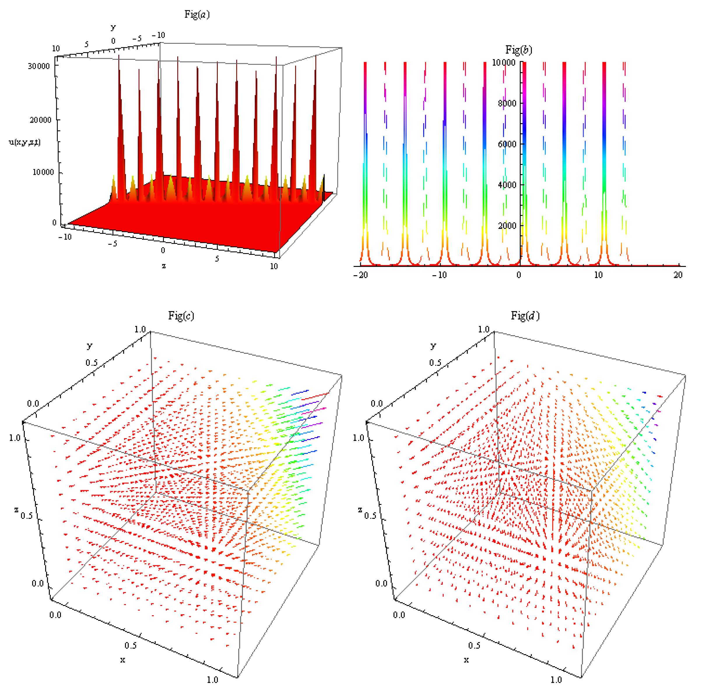
5. Physical Interpretation and Discussion of Results

The results presented in this article differ from those obtained by various researchers because Equations (3) and (14) deviate from established methods. By assigning specific parameter values, distinct families of solutions for the ordinary differential Equations (3) and (14) have been obtained. The extended Zakharov–Kuznetsov equation has been investigated by many researchers through different techniques. The authors in [42,43] employed the extended tanh method, the sine-Gordon expansion method, and  ( 1 / G ) -expansion method to derive new periodic solitary wave solutions of the extended Zakharov–Kuznetsov equation. In reference [3], the authors applied the modified extended direct algebraic method and abundant wave solutions were established. In this study, several novel and innovative outcomes have been achieved which have not been previously documented.
The obtained solutions of the eZK equation are illustrated graphically to clarify their physical significance. The graphs of the acquired solutions consist of the bright–dark solitons, kink soliton, kink- and anti-kink-type breather waves, multi-peak solitons, and periodic solitary waves having different amplitudes. In Figure 1, by setting parameters to appropriate values, result (26) is obtained and illustrated. Figure 1a depicts the dark solitons, (b) their 2D cross-section, and (c,d) their electric field  E 1  and magnetic field  B 1 , respectively. In Figure 2, by setting parameters to appropriate values, result (27) is obtained and illustrated. Figure 2a depict the two-peak solitons, (b) their 2D cross-section, and (c,d) their electric field  E 2  and magnetic field  B 2 , respectively. By setting parameters to appropriate values, result (28) is obtained and illustrated. Figure 3a depicts the bright solitons, (b) their 2D cross-section, and (c,d) their electric field  E 3  and magnetic field  B 3 , respectively. In Figure 4, by setting parameters to appropriate values, result (29) is obtained and illustrated. Figure 4a depicts the multi-peak solitons, (b) their 2D cross-section, and (c,d) their electric field  E 4  and magnetic field  B 4 , respectively.
In Figure 5, by setting parameters to appropriate values, result (54) is obtained and illustrated. Figure 5a depicts the bright multi-peak solitons, (b) their 2D cross-section, and (c,d) their electric field  E 1  and magnetic field  B 1 , respectively. By setting parameters to appropriate values, the result (58) in Figure 6 is illustrated as: Figure 6a depicts the peak solitons, (b) their 2D cross-section, and (c,d) their electric field  E 2  and magnetic field  B 2 , respectively. In Figure 7, by setting parameters to appropriate values, the result (64) is illustrated as: Figure 7a depicts the bright-type peak solitons, (b) their 2D cross-section, and (c,d) their electric field  E 5  and magnetic field  B 5 , respectively. The relation in Equation (75) between  ν  and  δ 1 , δ 2 , and  δ 3  is shown in Figure 8.

6. Conclusions

We have effectively applied the presented techniques in this work to the (3+1)-dimensional eZK equation. This dynamical equation is used to describe nonlinear dust-ion-acoustic solitary waves of three dimensions in a magnetized two-ion-temperature dusty plasma. By using the projected methods on this dynamical model, various forms of analytical solutions, including solitons, solitary waves, rational solutions, trigonometric solutions, hyperbolic function solutions, and other wave solutions, have been developed in this research. It has been possible to obtain soliton solutions in a variety of shapes, including kink and anti-kink waves, dark and bright solitons, kink solitons, and multi-peak solitons, etc. With the help of software, the solitary wave results (that signify the electrostatic potential field), electric and magnetic fields, and quantum statistical pressures are also constructed. These solutions have numerous applications in various areas of applied sciences. Graphical representations of some of the obtained results, and the electric and magnetic fields as well as the electrostatic field potential are also presented. These results demonstrate the effectiveness of the proposed techniques, which will also be useful in solving many other nonlinear physical models that arise in several diverse areas of applied sciences.

Author Contributions

Methodology and Software M.A.; Resources and formal analysis, M.T.; Supervision and Validation, A.R.S.; writing—review and editing and Conceptualization, F.Y. All authors have read and agreed to the published version of the manuscript.

Funding

Deputyship for Research and Innovation, Ministry of Education in Saudi Arabia for funding this research work the project number: 445-9-342.

Data Availability Statement

MDPI Research Data Policies.

Acknowledgments

The authors extend their appreciation to the Deputyship for Research and Innovation, Ministry of Education in Saudi Arabia for funding this research work through project number: 445-9-342. Furthermore, the authors would like to extend their appreciation to Taibah University for its supervision support.

Conflicts of Interest

The authors declare no conflict of interest.

References

  1. Qian, X.; Lu, D.; Arshad, M.; Shehzad, K. Novel traveling wave solutions and stability analysis of perturbed Kaup-Newell Schrödinger dynamical model and its applications. Chin. Phys. B 2021, 30, 020201. [Google Scholar] [CrossRef]
  2. Shehzad, K.; Seadawy, A.R.; Wang, J.; Arshad, M. Multi peak solitons and btreather types wave solutions of unstable NLSEs with stability and applications in optics. Opt. Quantum Electron. 2023, 55, 1–18. [Google Scholar] [CrossRef]
  3. Lu, D.; Seadawy, A.R.; Arshad, M.; Wang, J. New solitary wave solutions of (3+1)-dimensional nonlinear extended Zakharov-Kuznetsov and modified KdV-Zakharov-Kuznetsov equations and their applications. Results Phys. 2017, 7, 899–909. [Google Scholar] [CrossRef]
  4. Zakharov, V.E.; Kuznetsov, E.A. On three dimensional solitons. Zhurnal Eksp. Teoret. Fiz 1974, 66, 594–597. [Google Scholar]
  5. Biswas, A.; Zerrad, E. Solitary wave solution of the Zakharov–Kuznetsov equation in plasmas with power law nonlinearity. Nonlinear Anal. Real World Appl. 2010, 11, 3272–3274. [Google Scholar] [CrossRef]
  6. Krishnan, E.V.; Biswas, A. Solutions to the Zakharov-Kuznetsov equation with higher order nonlinearity by mapping and ansatz methods. Phys. Wave Phenom. 2010, 18, 256–261. [Google Scholar] [CrossRef]
  7. Suarez, P.; Biswas, A. Exact 1-soliton solution of the Zakharov equation in plasmas withpower law nonlinearity. Appl. Math. Comput. 2011, 217, 7372–7375. [Google Scholar] [CrossRef]
  8. Johnpillai, A.G.; Kara, A.H.; Biswas, A. Symmetry Solutions and Reductions of a Class of Generalized. 2 C 1/-dimensional Zakharov–Kuznetsov Equation. Int. J. Nonlinear Sci. Numer. Simul. 2011, 12, 45–50. [Google Scholar] [CrossRef]
  9. Ebadi, G.; Mojaver, A.; Milovic, D.; Johnson, S.; Biswas, A. Solitons and other solutions to the quantum Zakharov-Kuznetsov equation. Astrophys. Space Sci. 2012, 341, 507–513. [Google Scholar] [CrossRef]
  10. Morris, R.; Kara, A.H.; Biswas, A. Soliton solution and conservation laws of the Zakharov equation in plasmas with power law nonlinearity. Nonlinear Anal. Model. Control 2013, 18, 153–159. [Google Scholar] [CrossRef]
  11. Kadomtsev, B.B.; Petviashvili, V.I. On the stability of solitary waves in weakly dispersing media. In Doklady Akademii Nauk; Russian Academy of Sciences: Moscow, Russia, 1970; Volume 192, pp. 753–756. [Google Scholar]
  12. Liu, Z.M.; Duan, W.S.; He, G.J. Effects of dust size distribution on dust acoustic waves in magnetized two-ion-temperature dusty plasmas. Phys. Plasmas 2008, 15, 083702. [Google Scholar] [CrossRef]
  13. Seadawy, A.R. Stability analysis for two-dimensional ion-acoustic waves in quantum plasmas. Phys. Plasmas 2014, 21, 052107. [Google Scholar] [CrossRef]
  14. Seadawy, A.R. Nonlinear wave solutions of the three-dimensional Zakharov–Kuznetsov–Burgers equation in dusty plasma. Phys. A Stat. Mech. Appl. 2015, 439, 124–131. [Google Scholar] [CrossRef]
  15. Abdullah; Seadawy, A.R.; Wang, J. Three-dimensional nonlinear extended Zakharov-Kuznetsov dynamical equation in a magnetized dusty plasma via acoustic solitary wave solutions. Braz. J. Phys. 2019, 49, 67–78. [Google Scholar] [CrossRef]
  16. Wang, G.W.; Xu, T.Z.; Johnson, S.; Biswas, A. Solitons and Lie group analysis to an extended quantum Zakharov–Kuznetsov equation. Astrophys. Space Sci. 2014, 349, 317–327. [Google Scholar] [CrossRef]
  17. Zhang, B.G.; Liu, Z.R.; Xiao, Q. New exact solitary wave and multiple soliton solutions of quantum Zakharov–Kuznetsov equation. Appl. Math. Comput. 2010, 217, 392–402. [Google Scholar] [CrossRef]
  18. Pakzad, H.R. Soliton energy of the Kadomtsev–Petviashvili equation in warm dusty plasma with variable dust charge, two-temperature ions, and nonthermal electrons. Astrophys. Space Sci. 2010, 326, 69–75. [Google Scholar] [CrossRef]
  19. Korteweg, D.J.; De Vries, G., XLI. On the Change of Form of Long Waves advancing in a Rectangular Canal, and on a New Type of Long Stationary Waves. Philos. Mag. 2011, 91, 1007–1028. [Google Scholar] [CrossRef]
  20. Yu, X.; Gao, Y.T.; Sun, Z.Y.; Liu, Y. N-soliton solutions, Bäcklund transformation and Lax pair for a generalized variable-coefficient fifth-order Korteweg–de Vries equation. Phys. Scr. 2010, 81, 045402. [Google Scholar] [CrossRef]
  21. Hirota, R. Exact solution of the Korteweg—de Vries equation for multiple collisions of solitons. Phys. Rev. Lett. 1971, 27, 1192. [Google Scholar] [CrossRef]
  22. Alam, M.N.; Hafez, M.G.; Akbar, M.A. Exact traveling wave solutions to the (3+1)-dimensional mKdV–ZK and the (2+1)-dimensional Burgers equations via exp (-ϕ(η))-expansion method. Alex. Eng. J. 2015, 54, 635–644. [Google Scholar] [CrossRef]
  23. Abdou, M.A. The extended tanh method and its applications for solving nonlinear physical models. Appl. Math. Comput. 2007, 190, 988–996. [Google Scholar] [CrossRef]
  24. Xu, G.; Li, Z. Exact travelling wave solutions of the Whitham–Broer–Kaup and Broer–Kaup–Kupershmidt equations. Chaos Solitons Fractals 2005, 24, 549–556. [Google Scholar] [CrossRef]
  25. Wen, X. Construction of new exact rational form non-travelling wave solutions to the (2+1)-dimensional generalized Broer–Kaup system. Appl. Math. Comput. 2010, 217, 1367–1375. [Google Scholar] [CrossRef]
  26. Zeng, X.; Wang, D.S. A generalized extended rational expansion method and its application to (1+1)-dimensional dispersive long wave equation. Appl. Math. Comput. 2009, 212, 296–304. [Google Scholar] [CrossRef]
  27. Yao, Y. Abundant families of new traveling wave solutions for the coupled Drinfel’d–Sokolov–Wilson equation. Chaos Solitons Fractals 2005, 24, 301–307. [Google Scholar] [CrossRef]
  28. Peng, Y.Z. Exact solutions for some nonlinear partial differential equations. Phys. Lett. A 2003, 314, 401–408. [Google Scholar] [CrossRef]
  29. Ugurlu, Y.; Kaya, D.; Inan, I.E. Comparison of three semi-analytical methods for solving (1+1)-dimensional dispersive long wave equations. Comput. Math. Appl. 2011, 61, 1278–1290. [Google Scholar] [CrossRef]
  30. Dinarv, S.; Khosravi, S.; Doosthoseini, A.; Rashidi, M.M. The homotopy analysis method for solving the Sawada-Kotera and Lax’s fifth-order KdV equations. Adv. Theor. Appl. Mech. 2008, 1, 327–335. [Google Scholar]
  31. Biazar, J.; Badpeima, F.; Azimi, F. Application of the homotopy perturbation method to Zakharov–Kuznetsov equations. Comput. Math. Appl. 2009, 58, 2391–2394. [Google Scholar] [CrossRef]
  32. Kanth, A.R.; Aruna, K. Differential transform method for solving the linear and nonlinear Klein–Gordon equation. Comput. Phys. Commun. 2009, 180, 708–711. [Google Scholar] [CrossRef]
  33. Rashidi, M.M.; Erfani, E. Traveling wave solutions of WBK shallow water equations by differential transform method. Adv. Theor. Appl. Mech. 2010, 3, 263–271. [Google Scholar]
  34. Keskin, Y.; Oturanc, G. Reduced differential transform method for partial differential equations. Int. J. Nonlinear Sci. Numer. Simul. 2009, 10, 741–750. [Google Scholar] [CrossRef]
  35. Abazari, R.; Abazari, M. Numerical simulation of generalized Hirota–Satsuma coupled KdV equation by RDTM and comparison with DTM. Commun. Nonlinear Sci. Numer. Simul. 2012, 17, 619–629. [Google Scholar] [CrossRef]
  36. Seadawy, A.R. New exact solutions for the KdV equation with higher order nonlinearity by using the variational method. Comput. Math. Appl. 2011, 62, 3741–3755. [Google Scholar] [CrossRef]
  37. Wang, M.; Li, X.; Zhang, J. The (G′/G)-expansion method and travelling wave solutions of nonlinear evolution equations in mathematical physics. Phys. Lett. A 2008, 372, 417–423. [Google Scholar] [CrossRef]
  38. Guo, S.; Zhou, Y. The extended (G′/G)-expansion method and its applications to the Whitham–Broer–Kaup–Like equations and coupled Hirota–Satsuma KdV equations. Appl. Math. Comput. 2010, 215, 3214–3221. [Google Scholar] [CrossRef]
  39. Lü, H.L.; Liu, X.Q.; Niu, L. A generalized (G′/G)-expansion method and its applications to nonlinear evolution equations. Appl. Math. Comput. 2010, 215, 3811–3816. [Google Scholar] [CrossRef]
  40. Li, L.X.; Li, E.Q.; Wang, M.L. The (G′/G,1/G)-expansion method and its application to travelling wave solutions of the Zakharov equations. Appl.-Math.-A J. Chin. Univ. 2010, 25, 454–462. [Google Scholar] [CrossRef]
  41. Wang, J.; Shehzad, K.; Seadawy, A.R.; Arshad, M.; Asmat, F. Dynamic study of multi-peak solitons and other wave solutions of new coupled KdV and new coupled Zakharov–Kuznetsov systems with their stability. J. Taibah Univ. Sci. 2023, 17, 2163872. [Google Scholar] [CrossRef]
  42. Wazwaz, A.M. The extended tanh method for the Zakharov–Kuznetsov (ZK) equation, the modified ZK equation, and its generalized forms. Commun. Nonlinear Sci. Numer. Simul. 2008, 13, 1039–1047. [Google Scholar] [CrossRef]
  43. Ali, K.K.; Yilmazer, R.; Yokus, A.; Bulut, H. Analytical solutions for the (3+1)-dimensional nonlinear extended quantum Zakharov–Kuznetsov equation in plasma physics. Phys. A Stat. Mech. Appl. 2020, 548, 124327. [Google Scholar] [CrossRef]
Figure 1. By setting parameters to appropriate values, result (26) is obtained. (a) Depicts the dark solitons, (b) their 2D cross-section, and (c,d) its electric field  E 1  and magnetic field  B 1 , respectively.
Fractalfract 07 00691 g001
Figure 2. By setting parameters to appropriate values, result (27) is obtained. (a) Depicts the two-peak solitons, (b) their 2D cross-section, and (c,d) their electric field  E 2  and magnetic field  B 2 , respectively.
Fractalfract 07 00691 g002
Figure 3. By setting parameters to appropriate values, result (28) is obtained. (a) Depicts the bright solitons, (b) their 2D cross-section, and (c,d) their electric field  E 3  and magnetic field  B 3 , respectively.
Fractalfract 07 00691 g003
Figure 4. By setting parameters to appropriate values, result (29) is obtained. (a) Depicts the multi-peak solitons of diverse amplitudes, (b) their 2D cross-section, and (c,d) their electric field  E 4  and magnetic field  B 4 , respectively.
Fractalfract 07 00691 g004
Figure 5. By setting parameters to appropriate values, result (54) is obtained. (a) Depicts the bright multi-peak solitons, (b) their 2D cross-section, and (c,d) their electric field  E 1  and magnetic field  B 1 , respectively.
Fractalfract 07 00691 g005
Figure 6. By setting parameters to appropriate values, result (58) is obtained. (a) Depicts the peak solitons having diverse amplitudes, (b) their 2D cross-section, and (c,d) their electric field  E 2  and magnetic field  B 2 , respectively.
Fractalfract 07 00691 g006
Figure 7. By setting parameters to appropriate values, the result (64) is obtained. (a) Depicts the bright-type peak solitons having diverse amplitudes, (b) their 2D cross-section, and (c,d) their electric field  E 5  and magnetic field  B 5 , respectively.
Fractalfract 07 00691 g007
Figure 8. The relation in Equation (75) between  ν  and  δ 1 , δ 2 , and  δ 3  is shown in (a,b) (three- and two-dimensional) respectively.
Fractalfract 07 00691 g008
Disclaimer/Publisher’s Note: The statements, opinions and data contained in all publications are solely those of the individual author(s) and contributor(s) and not of MDPI and/or the editor(s). MDPI and/or the editor(s) disclaim responsibility for any injury to people or property resulting from any ideas, methods, instructions or products referred to in the content.

