Highly Efficient Numerical Algorithm for Nonlinear Space Variable-Order Fractional Reaction–Diffusion Models

Abstract

In this paper, we present a new highly efficient numerical algorithm for nonlinear variable-order space fractional reaction–diffusion equations. The algorithm is based on a new method developed by using the Gaussian quadrature pole rational approximation. A splitting technique is used to address the issues related to computational efficiency and the stability of the method. Two linear systems need to be solved using the same real-valued discretization matrix. The stability and convergence of the method are discussed analytically and demonstrated through numerical experiments by solving test problems from the literature. The variable-order diffusion effects on the solution profiles are illustrated through graphs. Finally, numerical experiments demonstrate the superiority of the presented method in terms of computational efficiency, accuracy, and reliability.

1. Introduction

The numerical study of variable-order fractional partial differential equations (VOFDEs) is comparatively new and still in its early stages. It has applications in almost all areas of science and engineering, including elasticity [1], geothermal heat transport [2], biochemistry [3], porous or fractured media [4], the blood alcohol model [5], anomalous diffusion [6,7,8], viscoelastic mechanics [9], control systems [10], petroleum engineering [11], and many other areas of physics and engineering [12].

Constant-order fractional calculus [13,14] can handle certain extremely significant physical phenomena, but it cannot handle some important classes of physical situations where the order of the fractional derivative is variable. For example, in protein reaction kinetics, it has been found that there are relaxation processes that are adequately represented by a fractional order [15], which depends on the temperature [15]. As a result, the basic physics of reaction kinetics (represented by the order of the relaxation mechanism) change with respect to changes in the temperature. It is logical to suppose that the protein kinetics will be better described by a differential equation with operators that update their order as a function of temperature. To encourage the use of variable-order fractional operators, we can find more examples in the literature. Electroviscous or electrorheological fluids [16] and polymer gels [17] have been shown to change their properties in response to variations in the strength of an applied electric field. The properties of magnetorheological elastomers change in response to the strength of the magnetic field [18]. In the field of damage modeling, nonlinear stress/strain behavior has been shown to change as damage accumulates (over time) in a structure. Variable-order computations may be better suited to describe this phenomenon. These examples suggest that variable-order operators are better suited to represent certain types of physical problems.

The fascinating extension of fractional calculus known as variable-order fractional calculus was proposed by Samko [19] in 1993. The non-stationary power law kernel of variable-order fractional operators allows them to represent the memory and inheritance properties of a variety of physical phenomena and processes. Variable-order fractional calculus has, therefore, been used as a viable option to provide an efficient mathematical framework for the precise characterization of complicated physical systems and processes.

A challenging task for researchers in the study of fractional differential equations is to find the exact solution of the dynamical systems. In most cases, we do not know the exact solution to the problem and must search for a numerical approximation. The numerical study of variable-order fractional partial differential equations is comparatively new and is still at a young stage. In general, numerical methods are used to approximate solutions of VOFDEs. Due to the complexity of fractional operators, finding the numerical solution of nonlinear problems is always a challenging task for researchers.

Lin et al. [20] presented the equality relation between the Riemann–Liouville fractional derivative and the Grünwald–Letnikov expansion with the variable-order fractional derivative. Exploiting this relationship, they proposed an explicit finite difference approximation for a one-dimensional variable-order fractional nonlinear reaction–diffusion problem. The convergence and stability of this approximation were proved. Zhuang et al. [8] proposed explicit and implicit Euler approximations for a one-dimensional advection–diffusion equation of a variable-order fractional derivative with a nonlinear source component on a finite domain. Sun et al. [21] studied the time variable-order fractional diffusion equation and proposed finite difference schemes. Farnaz et al. [22] applied the compact finite difference operator weighted-shifted Grünwald formula on the time fractional VOFDEs. In [23], the coupled nonlinear Ginzburg–Landau equations are formulated using the Heydari–Hosseininia concept’s nonsingular variable-order fractional derivative. The shifted Vieta–Lucas polynomials are used to build a numerical scheme. The authors of [24] derived the numerical scheme based on hp-version spectral collocation methods of the variable-order fractional approach. Based on a natural generalization of the classic Riesz potential, Darve et al. [25] developed a unique definition of the variable-order fractional Laplacian on ${\mathbb{R}}^n$. To explain the kernels of derivatives and the solution of a relaxation equation, a numerical approach for the numerical inversion of the Laplace transform is used in [26]. In [27], the authors suggested a technique for solving a generic variable-order temporal fractional advection–reaction–diffusion equation with complicated geometries using the meshless approach. For the nonlinear variable-order space fractional reaction–diffusion equations, Li and Wu [28] proposed an iterative reproducing kernel method.

In this paper, we consider the following two-dimensional variable-order initial boundary value problem:

$$\frac{\partial u(x,y,t)}{\partial t}={\mathcal{K}}_x\frac{{\partial }^{\alpha (x,t)}u(x,y,t)}{{\partial \left|x\right|}^{\alpha (x,t)}}+{\mathcal{K}}_y\frac{{\partial }^{\beta (y,t)}u(x,y,t)}{{\partial \left|y\right|}^{\beta (y,t)}}+F(u,t),$$

(1)

with initial and boundary conditions

$$\begin{array}{ccc}\hfill u(x,y,0)& =\phi (x,y),(x,y)\in [a,b]\times [c,d],\hfill & \end{array}$$

(2)

$$\begin{array}{cc}\hfill u(x,y,t)& =0,(x,y)\in \partial \Omega ,0<t,\hfill \end{array}$$

(3)

where $1<\alpha (x,t),\beta (y,t)<2$, $\Omega =(a,b)\times (c,d)$, ${\mathcal{K}}_x$ and ${\mathcal{K}}_y$ are diffusion coefficients. For $\alpha (x,t)=\beta (y,t)=2$, Equation (1) represents the two-dimensional classical reaction–diffusion model. The source term $F(u,t)$ is assumed to be continuous and satisfies the Lipschitz condition with $L>0$; that is:

$$\parallel F\left(u\right)-F\left(\tilde{u}\right)\parallel \le L\parallel u-\tilde{u}\parallel .$$

The space fractional derivative in Equation (1) is considered a Riesz fractional derivative of the variable order [12,29], defined as

$$\frac{{\partial }^{\alpha (x,t)}u(x,y,t)}{{\partial \left|x\right|}^{\alpha (x,t)}}=\frac{-1}{2cos\left(\frac{\pi \alpha (x,t)}{2}\right)}\left[{}_{RL}{\mathrm{D}}_{a,x}^{\alpha (x,t)}+{}_{RL}{\mathrm{D}}_{x,b}^{\alpha (x,t)}\right]u(x,y,t),$$

(4)

$$\frac{{\partial }^{\beta (y,t)}u(x,y,t)}{{\partial \left|y\right|}^{\beta (y,t)}}=\frac{-1}{2cos\left(\frac{\pi \beta (y,t)}{2}\right)}\left[{}_{RL}{\mathrm{D}}_{c,y}^{\beta (y,t)}+{}_{RL}{\mathrm{D}}_{y,d}^{\beta (y,t)}\right]u(x,y,t),$$

(5)

where ${}_{RL}{\mathrm{D}}_{a,x}^{\alpha (x,t)}$, ${}_{RL}{\mathrm{D}}_{c,y}^{\beta (y,t)}$ are the left variable-order Riemann–Liouville fractional derivatives, defined as follows:

$${}_{RL}{\mathrm{D}}_{a,x}^{\alpha (x,t)}u(x,y,t)=\frac{1}{\Gamma (2-\alpha (x,t\left)\right)}\frac{{\partial }^2}{\partial x^2}{\int }_a^x{(x-\tau )}^{1-\alpha (x,t)}u(\tau ,y,t)\mathrm{d}\tau ,$$

(6)

$${}_{RL}{\mathrm{D}}_{c,y}^{\beta (y,t)}u(x,y,t)=\frac{1}{\Gamma (2-\beta (y,t\left)\right)}\frac{{\partial }^2}{\partial y^2}{\int }_c^y{(y-\xi )}^{1-\beta (y,t)}u(x,\xi ,t)\mathrm{d}\xi .$$

(7)

Similarly, the right variable-order Riemann–Liouville fractional derivatives ${}_{RL}{\mathrm{D}}_{x,b}^{\alpha (x,t)}$, ${}_{RL}{\mathrm{D}}_{y,d}^{\beta (y,t)}$ are defined as

$${}_{RL}{\mathrm{D}}_{x,b}^{\alpha (x,t)}u(x,y,t)=\frac{1}{\Gamma (2-\alpha (x,t\left)\right)}\frac{{\partial }^2}{\partial x^2}{\int }_x^b{(x-\tau )}^{1-\alpha (x,t)}u(\tau ,y,t)\mathrm{d}\tau ,$$

(8)

$${}_{RL}{\mathrm{D}}_{y,d}^{\beta (y,t)}u(x,y,t)=\frac{1}{\Gamma (2-\beta (y,t\left)\right)}\frac{{\partial }^2}{\partial y^2}{\int }_y^d{(y-\xi )}^{1-\beta (y,t)}u(x,\xi ,t)\mathrm{d}\xi ,$$

(9)

respectively.

The variable-order fractional model (1) allows different diffusion rates of the fractional order with respect to each spatial variable as well as time. To explain the generalized diffusion fluxes that do not satisfy Fick’s law, Fourier’s law, or Newton’s constitutive equation, the Riesz fractional derivative is introduced. Since they connect the local state of the field with the state of the whole field, these nonlocal derivatives can improve the predictability of several models. For more on fractional Riesz derivatives and fractional Laplacian, see [19,29].

To our knowledge, there is no work on variable-order space fractional problems by a third-order time-stepping method. However, for the constant-order fractional differential equations, several approaches have been developed to solve space-fractional reaction–diffusion equations. Khaliq et al. [30] presented a fourth-order technique for the space-fractional nonlinear Schrödinger equation. The authors of [31] presented a numerical approach for solving variable-order fractional differential equations utilizing fractional-order generalized Chelyshkov wavelets and the beta function. Ding and his collaborators [32,33] developed a numerical technique by discretizing the Riesz derivative; they produced interesting findings by adopting the Runge–Kutta (ETDRK) approach, the Padé approximation, or by developing new helpful generating functions in a series of articles. Furati et al. [34] developed two schemes for one-dimensional space fractional reaction–diffusion equations. Yousuf et al. [35] provided an L-stable method and an A-stable method for solving two-dimensional nonlinear fractional reaction–diffusion problems. The authors of this study [36] suggested finite difference techniques for solving Riesz-space variable-order fractional diffusion equations. The time derivatives in linear and nonlinear situations are then discretized using the Crank–Nicolson and linearly implicit difference schemes, respectively.

Almost all previously developed time-stepping methods used Padé rational approximations, which required numerical computations with complex numbers that made the methods slow and computationally expensive. Motivated by the above-mentioned work, the natural question is: Is there any way to develop a time-stepping method for variable-order fractional problems without using Padé rational approximations? The answer to this question is efficiently presented in this work. In this paper, we develop an unconditionally stable, highly efficient, third-order convergent numerical method for nonlinear variable-order fractional reaction–diffusion problems. Instead of using Padé approximations, a rational approximation with a single Gaussian quadrature pole, called the Calahan rational approximation [37], is used to avoid complex arithmetic. To achieve high accuracy and computational efficiency, one must solve two linear systems of the form $(kA+cI)X=Y$ using the Gaussian quadrature point $c=\frac{3+\sqrt{3}}{6}$ and the same discretization matrix A. For example, the rational approximation Padé-(2, 2) has two complex conjugate poles and residues and Padé-(0, 4) has two pairs of complex conjugate poles and residues. To achieve the desired results, multiple systems with differing coefficient matrices must be solved. This process can also necessitate complex arithmetic, potentially making the schemes more computationally expansive. The computational efficiency of the new method is shown by recording the central processing unit (CPU) time for each iteration in the convergence tables.

The rest of this paper is organized as follows: Section 2 is devoted to the discretization of the Riesz derivative. In Section 3, a new third-order numerical method for nonlinear space variable-order reaction–diffusion problems is developed and an algorithm is provided to easily implement the method. The stability of the method and a linear error analysis are given in Section 4. In Section 5, numerical experiments are performed by solving nonlinear reaction–diffusion problems with the variable-order fractional Riesz derivative. The convergence results and CPU time are also presented in the same section. Finally, our conclusion is drawn in the last section.

2. Spatial Discretization

In this section, we provide the space derivative approximation of Equation (1). Suppose that $u^{(m-1)}\in \mathrm{C}[a,b]$ and $u^{\left(m\right)}$ are integrable in $[a,b]$. Consider the spatial discretization: $x_m=a+m{h}_x$, $m=0,1,\cdots ,M$ with $h_x=(b-a)/M$ and $y_n=c+n{h}_y$, $n=0,1,\cdots ,N$ with $h_y=(d-c)/N$. Then for every $\alpha (x,t)\in (1,2)$, the variable-order Riemann–Liouville fractional derivative exists and coincides with the Grünwald–Letnikov derivative. The relationship between the Riemann–Liouville and Grünwald–Letnikov definitions also plays an essential role in the numerical approximations of fractional differential equations, the manipulation of fractional derivatives, and the formulation of physically meaningful initial-value and boundary-value problems for fractional differential equations. As a result, the Riemann–Liouville definition can be used to formulate the problems, and the Grünwald–Letnikov definition can then be applied to arrive at a numerical solution. The left and right variable-order Grünwald–Letnikov fractional derivatives [29] are defined as follows:

$${}_{GL}{\mathrm{D}}_{a,x}^{\alpha (x,t)}u(x,y,t)=\underset{h_x\to 0^{+}}{lim}{h}_x^{-\alpha (x,t)}{\displaystyle \sum _{k=0}^{\frac{x-a}{h_x}}}{(-1)}^k\frac{\Gamma \left(\alpha \right(x,t)+1)}{k!\Gamma \left(\alpha \right(x,t)-k+1)}u(x-k{h}_x,y,t),$$

and

$${}_{GL}{\mathrm{D}}_{x,b}^{\alpha (x,t)}u(x,y,t)=\underset{h_x\to 0^{+}}{lim}{h}_x^{-\alpha (x,t)}{\displaystyle \sum _{k=0}^{\frac{b-x}{h_x}}}{(-1)}^k\frac{\Gamma \left(\alpha \right(x,t)+1)}{k!\Gamma \left(\alpha \right(x,t)-k+1)}u(x+k{h}_x,y,t),$$

respectively. In [38], the symmetrical fractional central difference operator ${\Delta }_{h_x}^{\alpha }$ for the constant fractional order $\alpha$ is introduced by Ortigueira. By changing the constant-order $\alpha$ with variable-order $\alpha (x,t)$ we have

$${\Delta }_{h_x}^{\alpha (x,t)}u(x,y,t)={\displaystyle \sum _{k=-\infty }^{\infty }}\frac{{(-1)}^k\Gamma (\alpha (x,t)+1)}{\Gamma (\frac{\alpha (x,t)}{2}-k+1)\Gamma (\frac{\alpha (x,t)}{2}+k+1)}u(x-k{h}_x,y,t).$$

(10)

Lemma 1.

Let $u\in {\mathrm{C}}^5\left(\mathbb{R}\right)$ and all derivatives of u up to five belong to ${\mathrm{L}}_1\left(\mathbb{R}\right)$, and by using the above-mentioned variable-order fractional central difference operator ${\Delta }_{h_x}^{\alpha (x,t)}$, the variable-order Riesz derivative can be discretized as

$$\frac{{\partial }^{\alpha (x,t)}}{{\partial \left|x\right|}^{\alpha (x,t)}}u\left(x_j\right)=\frac{-1}{h_x^{\alpha (x,t)}}{\Delta }_{h_x}^{\alpha (x,t)}u\left(x_j\right)+\mathcal{O}\left(h_x^2\right).$$

Proof. 

The proof of this Lemma can be drawn by using a method similar to [39]. Therefore, we have chosen to omit the detailed proof here, inviting interested readers to explore it on their own. □

Lemma 2.

Let $p_j^{\alpha (x,t)}=\frac{{(-1)}^j\Gamma (\alpha (x,t)+1)}{\Gamma (\frac{\alpha (x,t)}{2}-j+1)\Gamma (\frac{\alpha (x,t)}{2}+j+1)}$ be the coefficient of the variable finite-centered difference approximation in Equation (10) for $j=0,\pm 1,\pm 2,\cdots ,$ and $\alpha (x,t)>-1.$ Then we have

• $p_0^{\alpha (x,t)}=\frac{\Gamma \left(\alpha \right(x,t)+1)}{{\Gamma }^2(\frac{\alpha (x,t)}{2}+1)},p_{j+1}^{\alpha (x,t)}=\left(1-\frac{\alpha (x,t)+1}{\frac{\alpha (x,t)}{2}+j+1}\right)p_j^{\alpha (x,t)},j=0,\pm 1,\pm 2,\cdots ,$
• $p_{-j}^{\alpha (x,t)}=p_j^{\alpha (x,t)}$, $p_0^{\alpha (x,t)}>0,$ $p_j^{\alpha (x,t)}\le 0$ for $j=\pm 1,\pm 2,\cdots ,$
• $p_j^{\alpha (x,t)}=\mathcal{O}\left(j^{-1-\alpha (x,t)}\right).$

Proof. 

This lemma can easily be proved by using the arguments in [39], (Lemma 2.1). Therefore, we have chosen to omit the detailed proof here, inviting interested readers to explore it on their own. □

When $u\left(x\right)=0$ for $x\notin (a,b)$, then $u_j=0$, for $j\ne 1,\cdots ,M-1$. At the interior mesh $x_m,m=1,\cdots ,M-1$, we have

$$\begin{array}{ccc}\hfill {\Delta }_{h_x}^{\alpha (x,t)}u\left(x_m\right)& =& {\displaystyle \sum _{j=m+1-M}^{m-1}}{p}_j^{\alpha (x,t)}u\left(x_{m-j}\right)\hfill \\ & =& \left[p_{m-1}^{\alpha (x,t)}{u}_1+p_0^{\alpha (x,t)}{u}_m+\cdots +p_{M-m-1}^{\alpha (x,t)}{u}_{M-1}\right].\hfill \end{array}$$

(11)

The system of Equation (11) can be written in the following form:

$${\Delta }_{h_x}^{\alpha (x,t)}U=P^{\alpha (x,t)}U$$

where

$$P^{\alpha (x,t)}=\left[\begin{array}{ccccccc}{p}_0^{\alpha (x,t)}& p_1^{\alpha (x,t)}& p_2^{\alpha (x,t)}& \cdots & p_{M-4}^{\alpha (x,t)}& p_{M-3}^{\alpha (x,t)}& p_{M-2}^{\alpha (x,t)}\\ p_1^{\alpha (x,t)}& p_0^{\alpha (x,t)}& p_1^{\alpha (x,t)}& \cdots & p_{M-5}^{\alpha (x,t)}& p_{M-4}^{\alpha (x,t)}& p_{M-3}^{\alpha (x,t)}\\ p_2^{\alpha (x,t)}& p_1^{\alpha (x,t)}& p_0^{\alpha (x,t)}& p_1^{\alpha (x,t)}& p_2^{\alpha (x,t)}& \cdots & p_{M-4}^{\alpha (x,t)}\\ ⋮& \ddots & \ddots & \ddots & \ddots & \ddots & ⋮\\ p_{M-4}^{\alpha (x,t)}& \cdots & p_2^{\alpha (x,t)}& p_1^{\alpha (x,t)}& p_0^{\alpha (x,t)}& p_1^{\alpha (x,t)}& p_2^{\alpha (x,t)}\\ p_{M-3}^{\alpha (x,t)}& p_{M-4}^{\alpha (x,t)}& \cdots & p_2^{\alpha (x,t)}& p_1^{\alpha (x,t)}& p_0^{\alpha (x,t)}& p_1^{\alpha (x,t)}\\ p_{M-2}^{\alpha (x,t)}& p_{M-3}^{\alpha (x,t)}& p_{M-4}^{\alpha (x,t)}& \cdots & p_2^{\alpha (x,t)}& p_1^{\alpha (x,t)}& p_0^{\alpha (x,t)}\end{array}\right],U=\left[\begin{array}{c}{u}_1\\ u_2\\ u_3\\ ⋮\\ u_{M-3}\\ u_{M-2}\\ u_{M-1}\end{array}\right].$$

The term $\frac{{\partial }^{\beta (y,t)}}{{\partial \left|y\right|}^{\beta (y,t)}}u(x,y,t)$ is similarly discretized. The semi-discrete system for Equation (1) is

$$\frac{\mathrm{d}\mathbf{u}}{\mathrm{d}\mathrm{t}}=\mathrm{A}\mathbf{u}+\mathrm{F}(\mathbf{u}\left(\mathrm{t}\right),\mathrm{t})$$

(12)

where $A={\mathcal{K}}_x{\Delta }_{h_x}^{\alpha (x,t)}\otimes I_x+I_y\otimes {\mathcal{K}}_y{\Delta }_{h_y}^{\beta (y,t)}$ is a square matrix of size $(M-1)(N-1)\times (M-1)(N-1)$, with $I_x$ and $I_y$ being identity matrices of sizes $(M-1)\times (M-1)$ and $(N-1)\times (N-1)$, respectively. Vector $\mathbf{u}$ is of the size $(M-1)(N-1)\times 1$ and consists of columns of the matrix $\left[u_{i,j}\right]$, where each $u_{i,j}=u\left(x_{,}{y}_j\right)$ for $1\le i\le M-1$, $1\le j\le N-1$. The nonlinear term $F\left(\mathbf{u}\right)={\left[F_1,\cdots ,F_{M-1}\right]}^T$ is a vector of size $(M-1)(N-1)\times 1$ with each $F_j={[F\left(u_{1,j}\right),F\left(u_{2,j}\right),\cdots ,F\left(u_{M-1,j}\right)]}^T,j=1,2,\cdots N-1$.

3. The Reaction–Diffusion System and Time-Stepping Method

Consider the following standard semi-linear initial value problem:

$$\begin{array}{ccc}\hfill \frac{\partial u}{\partial t}+Au& =& F(u,t)\mathrm{in}\Omega ,t\in \left(0,T\right],\hfill \\ \hfill u(x,y,0)& =& u_0\mathrm{in}\Omega ,\hfill \end{array}$$

(13)

where A represents a uniformly elliptic operator, F is taken as a smooth nonlinear function defined on ${\mathbf{R}}^d$, and $\Omega$ is a bounded domain in ${\mathbf{R}}^d$.

$$\begin{array}{c}\hfill Au:=-{\displaystyle \sum _{j,k=1}^d}\frac{\partial }{\partial x_j}\left(a_{j,k}\frac{\partial u}{\partial x_k}\right)+{\displaystyle \sum _{j=1}^d}{b}_j\frac{\partial u}{\partial x_j}+b_{0}u.\end{array}$$

(14)

Coefficients $a_{j,k}$ and $b_j$ are sufficiently smooth $C^{\infty }$ functions defined over $\overline{\Omega }$; they possess the properties $a_{j,k}=a_{k,j}$, and $b_0\ge 0$, and there exists some $c_0>0$,

$$\begin{array}{c}\hfill {\displaystyle \sum _{j,k=1}^d}{a}_{j,k}{\xi }_j{\xi }_k\ge c_0\left|{\xi }^2\right|,\mathrm{on}\overline{\Omega },\mathrm{for}\mathrm{all}\xi \in {\mathbf{R}}^d.\end{array}$$

(15)

We examine the initial value problem (12) in a Hilbert space $\mathcal{H}$, where the linear, self-adjoint, and positive-definite closed operator A with a compact inverse is defined on a dense domain $D\left(A\right)\subset \mathcal{H}$; see [37]. Operator A could represent any of ${\left\{A_{\overline{h}}\right\}}_{0<\overline{h}\le {\overline{h}}_0},$ resulting from a spatial discretization, and $\mathcal{H}$ could be an appropriate finite-dimensional subspace of $L_2(\Omega )$, cf. [37,40].

Assume that the resolvent set $\rho \left(A\right)$ satisfies

$$\rho \left(A\right)\supset {\overline{\Sigma }}_{\alpha },{\Sigma }_{\alpha }:=\{c\in \mathbb{C}:\alpha <|arg\left(c\right)|\le \pi ,c\ne 0\}.$$

for some $\alpha \in (0,\pi /2)$. We also assume that there exists $M\ge 1$, such that

$$\parallel {(cI-A)}^{-1}\parallel \le M|c^{-1}|,c\in {\Sigma }_{\alpha }.$$

(16)

It follows that $-A$ is the infinitesimal generator of an analytic semigroup ${\left\{e^{-tA}\right\}}_{t\ge 0}$, which is the solution operator for (13) with $F\equiv 0$. There is a standard representation,

$$e^{-tA}=\frac{1}{2\pi i}{\int }_{\Lambda }{e}^{-tc}{(cI-A)}^{-1}dc,$$

(17)

where $\Lambda :=\{c\in \mathbb{C}:|arg\left(c\right)|=\theta \}$, oriented so that $\mathrm{Im}\left(c\right)$ decreases, for any $\theta \in (\alpha ,\frac{\pi }{2})$. Using the integrating factor approach, we write the exact solution of (13) as a Volterra integral equation,

$$u\left(t\right)=e^{-tA}{u}_0+{\int }_0^t{e}^{-(t-s)A}F(u\left(s\right),s)ds.$$

(18)

Let $0<k\le k_0$, for some $k_0$, be the fixed time step and $t_n=nk$. We replace t with $t+k$ and apply the linear transformation $s-t=k\tau$ to transform (18) into the following nonlinear Fredholm integral equation,

$$\begin{array}{ccc}\hfill u(t+k)& =& e^{-kA}u\left(t\right)+k{\int }_0^1{e}^{-k(1-\tau )A}F(u(t+k\tau ),t+k\tau )d\tau ,\hfill \end{array}$$

(19)

and set the recurrence formula,

$$u\left(t_{n+1}\right)=e^{-kA}u\left(t_n\right)+k{\int }_0^1{e}^{-k(1-\tau )A}F(u(t_n+\tau k),t_n+\tau k)d\tau .$$

(20)

3.1. Time-Stepping Method

It is quite challenging to implement the recurrence Equation (20) because it involves a nonlinear function of the unknown function $u\left(t\right)$. Another computational difficulty is to efficiently compute the matrix exponential functions $e^{-kA}$ and $e^{-k(1-\tau )A}$. Various time-stepping schemes are available in the literature, where matrix exponential functions are computed using MATLAB command $expm\left(A\right)$. Through our numerical experiments, we find that computing the matrix exponential functions using the MATLAB command is expansive (time-consuming), especially when matrix A is non-diagonal.

These difficulties are resolved by approximating the nonlinear function $F(u,t)$ by some constant functions and approximating the matrix exponential functions using a third-order single Gaussian quadrature pole rational approximation. The method developed by using such a rational approximation does not require complex arithmetic, which definitely enhance the computational efficiency.

Development of the Time-Stepping Method

The time-stepping method is constructed using the following steps:

Step1: 

Assume $F(u,t)$ to be constant $F_n$ over each sub-interval $[t_n,t_{n+1}]$; that is, $F(u\left(t\right),t)\approx F_n=F(u\left(t_n\right),t_n)$ for $t\in [t_n,t_{n+1}]$. Then the exact computation of Equation (20) results in

$$\begin{array}{ccc}\hfill a_n& \approx & P_0\left(\frac{kA}{2}\right)u_n+\frac{k}{2}{P}_1\left(\frac{kA}{2}\right)F_n\hfill \end{array}$$

(21)

where $P_0\left(kA\right)=e^{-kA},P_1\left(kA\right)={(-kA)}^{-1}(e^{-kA}-I).$

Step2: 

Now, using $a_n$, we approximate $F(u\left(t\right),t)\approx 2F_n^a-F_n,\mathrm{for}t\in [t_n,t_{n+1}]$

and evaluate the formula (20) to obtain

$$\begin{array}{ccc}\hfill b_n& \approx & P_0\left(kA\right)u_n+k{P}_1\left(kA\right)(2F_n^a-F_n)\hfill \end{array}$$

(22)

where $F_n^a=F(a_n,t_n+k/2).$

Step3: 

Finally, using $a_n$ and $b_n$, we approximate the nonlinear function as

$$F(u\left(t\right),t)\approx F_n+(t-t_n)(-3F_n+4F_n^a-F_n^b)+\frac{{(t-t_n)}^2}{2}(F_n-2F_n^a+F_n^b),$$

for $t\in [t_n,t_{n+1}]$, we evaluate the integral, rearrange the terms, and obtain the following formula to compute $u_{n+1}$

$$\begin{array}{ccc}\hfill u_{n+1}& =& P_0\left(kA\right)u_n+k{P}_1\left(kA\right)F_n+k{P}_2\left(kA\right)(-3F_n+4F_n^a-F_n^b)\hfill \\ & +& 4k{P}_3\left(kA\right)(F_n-2F_n^a+F_n^b),\hfill \end{array}$$

(23)

where

$$\begin{array}{ccc}\hfill F_n^b& =& F(b_n,t_n+k),\hfill \\ \hfill P_2\left(kA\right)& =& {(-kA)}^{-2}(e^{-kA}-I+kA),\hfill \\ \hfill P_3\left(kA\right)& =& {(-kA)}^{-3}\left(e^{-kA}-I+kA-\frac{k^2{A}^2}{2}\right).\hfill \end{array}$$

This is a Runge–Kutta type time-stepping strategy and can easily be implemented when A is a scalar or a diagonal matrix without a zero entry on the diagonal. However, when A is a non-diagonal matrix, there can be computational difficulties in computing ${(-A)}^{-1}$ and ${(-A)}^{-3}$ if eigenvalues of A are close to zero. Another issue is to efficiently compute the matrix exponential functions, $e^{-kA}$ and $e^{-kA/2}$, when A is non-diagonal. These issues are resolved by approximating the matrix exponential functions using Calahan’s single real pole rational approximation [37], as

$$\begin{array}{ccc}\hfill R\left(z\right)& =& 1-\frac{z}{1+\frac{3+\sqrt{3}}{6}z}-\frac{\sqrt{3}}{6}\frac{z^2}{{(1+\frac{3+\sqrt{3}}{6}z)}^2}=\frac{6(6+2\sqrt{3}z-(1+\sqrt{3})z^2)}{{(6+(3+\sqrt{3})z)}^2}.\hfill \end{array}$$

(24)

Replacing $e^{-kA}$ by $R\left(kA\right)$ and $e^{-kA/2}$ by $R(kA/2)$, in Equations (21)–(23), we find that factors $A^{-1}$ and $A^{-3}$ are also canceled. The third-order accuracy of the approximation (24) is shown as follows

$$\begin{array}{ccc}\hfill e^{-z}& =& 1-z+\frac{1}{2}{z}^2-\frac{1}{6}{z}^3+\frac{1}{24}{z}^4+O\left(z^4\right),\hfill \\ \hfill R\left(z\right)& =& 1-z+\frac{1}{2}{z}^2-\frac{1}{6}{z}^3-\frac{\sqrt{3}}{36}{z}^4+O\left(z^4\right),\hfill \end{array}$$

$$\begin{array}{c}\hfill \parallel e^{-z}-R\left(z\right)\parallel =O\left(z^4\right).\end{array}$$

L-acceptability for the method is evident from the fact that [41],

$$E\left(y\right)\equiv {\left|D\left(iy\right)\right|}^2-{\left|N\left(iy\right)\right|}^2=(108+72\sqrt{3})y^4\ge 0,y\in \mathcal{R}.$$

A very small error constant; that is, the coefficient of the leading term in the error, $0.00644585578$, shows good accuracy of the approximation. The rational approximation $R\left(z\right)$ also satisfies the condition that $\left|R\right(z\left)\right|<1$ for all $z>0$ and $R\left(z\right)$ is a decreasing function on $(0,\infty )$ with $\left|R\right(\infty \left)\right|<1$. In fact, $R(\infty )=1-\sqrt{3}>-1$. One crucial advantage of this approximation is that its denominator is the square of a linear function with one real pole of multiplicity 2. We can easily implement the method by solving two systems of the form $(kA+cI)X=Y$, where $c=\frac{3+\sqrt{3}}{6}$. In the finite-dimensional case, when A is a positive-definite matrix, this means that the two systems have the same real values of the positive-definite matrix [37]. This is in contrast to the schemes developed by using Padé approximations. For example, Padé-(2, 2) has two complex conjugate poles and Padé-(0, 4) has two pairs of complex conjugate poles. Such schemes require complex arithmetic, which can make the scheme computationally expansive.

3.2. Modified Time-Stepping Method

We use the third-order Calahan approximation (24) of $e^{-z}$ to modify the method (21)–(23), as:

$$\begin{array}{ccc}\hfill u_{n+1}& =& R\left(z\right)u_n+{\Phi }_1\left(z\right)F_n+{\Phi }_2\left(z\right)F_n^a+{\Phi }_3\left(kA\right)F_n^b,\hfill \end{array}$$

(25)

where

$$\begin{array}{ccc}\hfill {\Phi }_1\left(z\right)& =& \frac{6k(1+(1+\sqrt{3})z)}{{(6+(3+\sqrt{3})z)}^2},\hfill \\ \hfill {\Phi }_2\left(z\right)& =& \frac{24k}{{(6+(3+\sqrt{3})z)}^2},\hfill \\ \hfill {\Phi }_3\left(z\right)& =& \frac{6k(1+(2+\sqrt{3})z)}{{(6+(3+\sqrt{3})z)}^2},\hfill \end{array}$$

and

$$\begin{array}{ccc}\hfill a_n& =& \tilde{R}\left(z\right)u_n+{\tilde{\Phi }}_1\left(z\right)F_n,\hfill \end{array}$$

(26)

$$\begin{array}{ccc}\hfill b_n& =& R\left(z\right)u_n+{\tilde{\Phi }}_2\left(z\right)\left(2F_n^a-F_n\right),\hfill \end{array}$$

(27)

with

$$\begin{array}{ccc}\hfill \tilde{R}\left(z\right)& =& \frac{6(24+4\sqrt{3}z-(1+\sqrt{3})z^2)}{{(12+(3+\sqrt{3})z)}^2},\hfill \\ \hfill {\tilde{\Phi }}_1\left(z\right)& =& \frac{6k(12+(3+2\sqrt{3})z)}{{(12+(3+\sqrt{3})z)}^2},\hfill \\ \hfill {\tilde{\Phi }}_2\left(z\right)& =& \frac{6k(6+(3+2\sqrt{3})z)}{{(6+(3+\sqrt{3})z)}^2}.\hfill \end{array}$$

The rational functions $R\left(z\right)$ and $\tilde{R}\left(z\right)$ are Calahan rational approximations of $e^{-z}$ and $e^{-z/2}$, respectively. The rational functions ${\tilde{\Phi }}_1\left(z\right)$ and ${\tilde{\Phi }}_2\left(z\right)$ are obtained by simplifying $P_1(z/2)$ and $P_1\left(z\right)$ in (21) and (22), respectively. The rational functions ${\Phi }_1\left(z\right)$, ${\Phi }_2\left(z\right)$, and ${\Phi }_3\left(z\right)$ are obtained from the second, third, and fourth terms of (23), respectively.

3.3. Split Version of the New Method

The use of rational approximation (24) resolves the issues of computing matrix exponential functions and computing matrix inverses $A^{-1}$ and $A^{-3}$ but it creates another issue of computing matrix polynomial inverses ${(6I+(3+\sqrt{3})kA)}^{-2}$ and ${(12I+(3+\sqrt{3})kA)}^{-2}$. This is handled by applying splitting techniques, as follows:

$$\begin{array}{ccc}\hfill R\left(z\right)& =& -0.7320508076+\frac{2.784609691}{z+1.267949192}-\frac{0.7461339179}{{(z+1.267949192)}^2},\hfill \\ \hfill {\Phi }_1\left(z\right)& =& \frac{0.7320508076}{z+1.267949192}-\frac{0.6602540378}{{(z+1.267949192)}^2},\hfill \\ \hfill {\Phi }_2\left(z\right)& =& \frac{0.2679491924}{{(z+1.267949192)}^2},\hfill \\ \hfill {\Phi }_3\left(z\right)& =& \frac{1.0}{z+1.267949192}-\frac{1.0}{{(z+1.267949192)}^2},\hfill \\ \hfill \tilde{R}\left(z\right)& =& -0.7320508076+\frac{5.569219382}{z+2.535898385}-\frac{2.984535672}{{(z+2.535898385)}^2},\hfill \\ \hfill {\tilde{\Phi }}_1\left(z\right)& =& \frac{1.732050808}{z+2.535898385}-\frac{1.176914536}{{(z+2.535898385)}^2},\hfill \\ \hfill {\tilde{\Phi }}_2\left(z\right)& =& \frac{1.732050808}{z+1.267949192}-\frac{0.5884572681}{{(z+1.267949192)}^2}.\hfill \end{array}$$

Let poles and residues for $u_{n+1}$ be denoted as

$$\begin{array}{ccc}\hfill {\omega }_0& =& -0.7320508076,{\omega }_1=2.784609691,{\omega }_2=-0.7461339179,\hfill \\ \hfill {\omega }_{11}& =& 0.7320508076,{\omega }_{12}=-0.6602540378,\hfill \\ \hfill {\omega }_{21}& =& 0.0000000000,{\omega }_{22}=0.2679491924,\hfill \\ \hfill {\omega }_{31}& =& 1.000000000,{\omega }_{32}=-1.000000000,\hfill \\ \hfill c_1& =& 1.267949192,\hfill \end{array}$$

and let poles and residues for $a_n$ and $b_n$ be denoted by

$$\begin{array}{ccc}\hfill {\tilde{\omega }}_0& =& -0.7320508076,{\tilde{\omega }}_1=5.569219382,{\tilde{\omega }}_2=-2.984535672,\hfill \\ \hfill {\tilde{\omega }}_{11}& =& 1.732050808,{\tilde{\omega }}_{12}=-1.176914536,\hfill \\ \hfill {\tilde{\omega }}_{21}& =& 1.732050808,{\tilde{\omega }}_{22}=-0.5884572681,\hfill \\ \hfill {\tilde{c}}_1& =& 2.535898385,{\tilde{c}}_2=1.267949192=c_1.\hfill \end{array}$$

Then we can rewrite it as

$$\begin{array}{ccc}\hfill R\left(z\right)& =& {\omega }_0+\frac{{\omega }_1}{(z+c_1)}+\frac{{\omega }_2}{{(z+c_1)}^2},\hfill \\ \hfill {\Phi }_1\left(z\right)& =& \frac{{\omega }_{11}}{(z+c_1)}+\frac{{\omega }_{12}}{{(z+c_1)}^2},\hfill \\ \hfill {\Phi }_2\left(z\right)& =& \frac{{\omega }_{22}}{{(z+c_1)}^2},\hfill \\ \hfill {\Phi }_3\left(z\right)& =& \frac{{\omega }_{31}}{(z+c_1)}+\frac{{\omega }_{32}}{{(z+c_1)}^2},\hfill \\ \hfill \tilde{R}\left(z\right)& =& {\tilde{\omega }}_0+\frac{{\tilde{\omega }}_1}{(z+{\tilde{c}}_1)}+\frac{{\tilde{\omega }}_2}{{(z+{\tilde{c}}_1)}^2},\hfill \\ \hfill {\tilde{\Phi }}_1\left(z\right)& =& \frac{{\tilde{\omega }}_{11}}{(z+{\tilde{c}}_1)}+\frac{{\tilde{\omega }}_{12}}{{(z+{\tilde{c}}_1)}^2},\hfill \\ \hfill {\tilde{\Phi }}_2\left(z\right)& =& \frac{{\tilde{\omega }}_{21}}{(z+c_1)}+\frac{{\tilde{\omega }}_{22}}{{(z+c_1)}^2},\hfill \end{array}$$

Using these split forms, methods (25)–(27) can be written as

$$\begin{array}{cc}\hfill u_{n+1}=& \left[{\omega }_0+\frac{{\omega }_1}{(z+c_1)}+\frac{{\omega }_2}{{(z+c_1)}^2}\right]u_n+\left[\frac{{\omega }_{11}}{(z+c_1)}+\frac{{\omega }_{1,2}}{{(z+c_1)}^2}\right]F_n\hfill \\ \hfill +& \left[\frac{{\omega }_{22}}{{(z+c_1)}^2}\right]F_n^a+\left[\frac{{\omega }_{31}}{(z+c_1)}+\frac{{\omega }_{32}}{{(z+c_1)}^2}\right]F_n^b,\hfill \end{array}$$

and

$$\begin{array}{ccc}\hfill a_n& =& \left[{\tilde{\omega }}_0+\frac{{\tilde{\omega }}_1}{(z+{\tilde{c}}_1)}+\frac{{\tilde{\omega }}_2}{{(z+{\tilde{c}}_1)}^2}\right]u_n+\left[\frac{{\tilde{\omega }}_{11}}{(z+{\tilde{c}}_1)}+\frac{{\tilde{\omega }}_{12}}{{(z+{\tilde{c}}_1)}^2}\right]F_n,\hfill \end{array}$$

(28)

$$\begin{array}{ccc}\hfill b_n& =& \left[{\omega }_0+\frac{{\omega }_1}{(z+c_1)}+\frac{{\omega }_2}{{(z+c_1)}^2}\right]u_n+\left[\frac{{\tilde{\omega }}_{21}}{(z+c_1)}+\frac{{\tilde{\omega }}_{22}}{{(z+c_1)}^2}\right]\left(2F_n^a-F_n\right).\hfill \end{array}$$

(29)

3.4. Algorithm

In this subsection, we provide the algorithm that we developed to implement the new method.

To compute $a_n$:

• Solve $(kA+{\tilde{c}}_{1}I)W={\tilde{\omega }}_2{u}_n+{\tilde{\omega }}_{12}{F}_n$ for W.
• Solve $(kA+{\tilde{c}}_{1}I)X={\tilde{\omega }}_1{u}_n+{\tilde{\omega }}_{11}{F}_n+W$ for X.
• Compute $a_n={\tilde{\omega }}_0{u}_n+X$.

To compute $b_n$:

• Solve $(kA+c_{1}I)W={\omega }_2{u}_n+{\tilde{\omega }}_{22}(2F_n^a-F_n)$ for W.
• Solve $(kA+c_{1}I)X={\omega }_1{u}_n+{\tilde{\omega }}_{21}(2F_n^a-F_n)+W$ for X.
• Compute $b_n={\omega }_0{u}_n+X$.

To compute $u_{n+1}$:

• Solve $(kA+c_{1}I)W={\omega }_2{u}_n+{\omega }_{12}{F}_n++{\omega }_{22}{F}_n^a+{\omega }_{32}{F}_n^b$ for W.
• Solve $(kA+c_{1}I)X={\omega }_1{u}_n+{\omega }_{11}{F}_n+{\omega }_{31}{F}_n^b+W$ for X.
• Compute $u_{n+1}={\omega }_0{u}_n+X$.

4. Stability Regions and Linear Error Analysis

The general strategy for the stability analysis of a numerical method, which uses a variety of techniques for the linear and nonlinear parts of the equation, is provided by considering the following nonlinear autonomous ODE [42],

$$\begin{array}{c}\hfill u_t=cu+F\left(u\right),\end{array}$$

(30)

where $F\left(u\right)$ is a nonlinear function of the complex-valued function u. Let $u_0=u\left(t_0\right)$ be a fixed point, such that $c{u}_0+F\left(u_0\right)=0.$ When we consider u as a perturbation of the fixed point $u_0$ and $\lambda =F^{\prime }\left(u_0\right)$, then the linearization results in the following equation are as follows:

$$\begin{array}{c}\hfill u_t=cu+\lambda u.\end{array}$$

(31)

We say that fixed point $u_0$ is stable if $\mathrm{R}\mathrm{e}(c+\lambda )<0$ [42]. When a numerical method is applied to (31), the regions of stability are determined by taking into account the ratio $u_{n+1}/u_n$. For this, we assume that $x=\lambda k$ and $y=ck$, where k is the time step size.

When applying this new method to solve (31), we obtain the ratio

$$R(x,y)=\frac{u_{n+1}}{u_n}=\frac{c_0+c_{1}x+c_2{x}^2+c_3{x}^3}{Den},$$

with

$$\begin{array}{ccc}\hfill Den& =& {(6+(3+\sqrt{3})y)}^4{(12+(3+\sqrt{3})y)}^2,\hfill \\ \hfill c_0& =& -216((19+11\sqrt{3})y^6+(120+70\sqrt{3})y^5+(102\sqrt{3}+168)y^4\hfill \\ & & -(204\sqrt{3}+360)y^3-(1224+756\sqrt{3})y^2-(1296+720\sqrt{3})y-864),\hfill \\ \hfill c_1& =& -216((19\sqrt{3}+33)y^5-(25\sqrt{3}+44)y^4-(918+534\sqrt{3})y^3\hfill \\ & & -(2220+1344\sqrt{3})y^2-(2016+1152\sqrt{3})y-1152),\hfill \\ \hfill c_2& =& -216((33+19\sqrt{3})y^4-(127\sqrt{3}+222)y^3-(990+582\sqrt{3})y^2\hfill \\ & & -(1044y+576\sqrt{3})y-576),\hfill \\ \hfill c_3& =& -216((-90\sqrt{3}-156)y^3-(474+276\sqrt{3})y^2-(216\sqrt{3}+396)y-144).\hfill \end{array}$$

Linear Error Analysis

In this subsection, we prove the third-order convergence of the method for the specific case. We demonstrate that our new method has a third-order local truncation error in time using the linearization of $\mathbf{F}\left(\mathbf{u}\right)$ by $\Lambda \mathbf{u}$. We consider the following linear semi-discretized linearized system

$$\frac{d\mathbf{u}}{dt}=-A\mathbf{u}+\Lambda \mathbf{u},$$

(32)

where A and $\Lambda$ are the linear spatial discretization matrices. The exact solution of (32) is

$$\mathbf{u}\left(t_{n+1}\right)=e^{k(\Lambda -A)}\mathbf{u}\left(t_n\right).$$

(33)

By applying (25) to (32), we obtain

$$\begin{array}{ccc}\hfill {\mathbf{u}}_{n+1}& =& {\left(6I+(3+\sqrt{3})kA\right)}^{-2}\times \hfill \\ & & \left[36I+12\sqrt{3}kA-(1+\sqrt{3})k^2{A}^2+6k\Lambda +6(1+\sqrt{3})k^2\Lambda A\right]u_n\hfill \\ & +& {\left(6I+(3+\sqrt{3})kA\right)}^{-2}\left[24k\Lambda a_n+6k\Lambda (1+(2+\sqrt{3})kA)b_n\right]\hfill \end{array}$$

(34)

where ${\mathbf{a}}_n$ and ${\mathbf{b}}_n$ are

$$\begin{array}{ccc}\hfill {\mathbf{a}}_n& =& {\left(12I+(3+\sqrt{3})kA\right)}^{-2}\times \hfill \\ & & \left[144I+24\sqrt{3}kA-6(1+\sqrt{3})k^2{A}^2+72k\Lambda +6(3+2\sqrt{3})k\Lambda A\right]u_n,\hfill \end{array}$$

(35)

$$\begin{array}{ccc}\hfill {\mathbf{b}}_n& =& {\left(6I+(3+\sqrt{3})kA\right)}^{-2}\times \hfill \\ & & \left[36I+12k(\sqrt{3}A+3\Lambda )-(1+\sqrt{3})k^2{A}^2+6(3+2\sqrt{3})k^2\Lambda A\right](2a_n-u_n),\hfill \end{array}$$

(36)

Using the following Taylor series expansions

$$\begin{array}{ccc}\hfill {\displaystyle \frac{1}{{(12+(3+\sqrt{3})z)}^2}}& =& \frac{1}{144}-\left(\frac{1}{288}\frac{\sqrt{3}}{864}\right)z+\left(\frac{1}{576}+\frac{\sqrt{3}}{1152}\right)z^2\hfill \\ & -& (\frac{1}{1152}+\frac{5\sqrt{3}}{10368})z^3+\left(\frac{35}{82944}+\frac{5\sqrt{3}}{20736}\right)z^4+\mathcal{O}\left(z^5\right),\hfill \end{array}$$

(37)

$$\begin{array}{ccc}\hfill {\displaystyle \frac{1}{{(6+(3+\sqrt{3})z)}^2}}& =& \frac{1}{36}-\left(\frac{1}{36}\frac{\sqrt{3}}{108}\right)z+\left(\frac{1}{36}+\frac{\sqrt{3}}{72}\right)z^2\hfill \\ & -& (\frac{1}{36}+\frac{5\sqrt{3}}{324})z^3+\left(\frac{35}{1296}+\frac{5\sqrt{3}}{324}\right)z^4+\mathcal{O}\left(z^5\right),\hfill \end{array}$$

(38)

Equation (34) is simplified as

$$\begin{array}{ccc}\hfill {\mathbf{u}}_{n+1}& =& [I+k(\Lambda -A)+k^2\left({\displaystyle \frac{{\Lambda }^2}{2}}-\Lambda A+{\displaystyle \frac{A^2}{2}}\right)+k^3\left({\displaystyle \frac{{\Lambda }^3}{6}}-{\displaystyle \frac{{\Lambda }^{2}A}{2}}+{\displaystyle \frac{\Lambda A^2}{2}}-{\displaystyle \frac{A^3}{6}}\right)\hfill \\ & +& k^4\left(-{\displaystyle \frac{{\Lambda }^4}{24}}+\left(\frac{5}{24}+\frac{\sqrt{3}}{9}\right){\Lambda }^{3}A-\left(\frac{1}{4}+\frac{\sqrt{3}}{6}\right){\Lambda }^2{A}^2+\cdots \right)+\cdots ]{\mathbf{u}}_{\mathbf{n}}.\hfill \end{array}$$

(39)

We rewrite the exact solution (33) using the Taylor series expansion of $e^{-z}$

$$\begin{array}{ccc}\hfill {\mathbf{u}}_{\mathbf{n}+\mathbf{1}}& =& [I+k(\Lambda -A)+k^2\left({\displaystyle \frac{{\Lambda }^2}{2}}-\Lambda A+{\displaystyle \frac{A^2}{2}}\right)+k^3\left({\displaystyle \frac{{\Lambda }^3}{6}}-{\displaystyle \frac{{\Lambda }^{2}A}{2}}+{\displaystyle \frac{\Lambda A^2}{2}}-{\displaystyle \frac{A^3}{6}}\right)\hfill \\ & +& k^4\left({\displaystyle \frac{{\Lambda }^4}{24}}-{\displaystyle \frac{{\Lambda }^{3}A}{6}}+{\displaystyle \frac{{\Lambda }^2{A}^2}{4}}-{\displaystyle \frac{\Lambda A^3}{6}}+{\displaystyle \frac{A^4}{24}}\right)+\mathcal{O}\left(k^5\right)]{\mathbf{u}}_{\mathbf{n}}\hfill \end{array}$$

(40)

It follows from (39) and (40) that the local truncation error is

$$\begin{array}{ccc}\hfill {\mathcal{E}}_{n+1}& =& \parallel {\mathbf{u}}_{\mathbf{n}+\mathbf{1}}-e^{-k(A-\Lambda )}{\mathbf{u}}_{\mathbf{n}}\parallel =\mathcal{O}\left(k^4\right).\hfill \end{array}$$

(41)

5. Numerical Experiments

In this section, we compute and discuss the solutions obtained by applying the new method to three well-known practical test problems, an enzyme kinetics equation, the Fisher equation, and the Allen–Cahn equation. The stability region of the proposed method is shown in Figure 1. First, we solve these first two problems in one dimension and plot the solutions at $t=1$ for each $\alpha (x,t)$. The surface plots given in Figure 2 and Figure 3 show the behaviors of the solutions at $t=1$ corresponding to fractional derivatives of variable-order $\alpha (x,t)$. Figure 4 shows the solution profiles of Section 5.1 using ETD Crank–Nicolson scheme at $t=1$ with 80 time and 160 time steps. Because of the A-stability of the ETD Crank-–Nicolson scheme, unwanted oscillations occur in the solution profile when initial data are non-smooth. Since the initial data are not smooth in Section 5.1 due to mismatched initial and boundary conditions, unwanted oscillations can be seen in the solution profiles shown in Figure 4. These oscillations reduce in magnitude by decreasing the time-step size. But this makes the scheme computationally more expansive. The graph of the initial condition of Section 5.2 is showing in Figure 5. Note that the graph of the solution profile in Figure 3 is rotated to make it more visible. Next, we solve the same problems in two dimensions and plot the solutions at $t=1$ corresponding to the fractional derivatives of variable orders $\alpha (x,t)$ and $\beta (y,t)$ with $1\le \alpha (x,t),\beta (y,t)\le 2$. For simplicity, functions $\alpha (x,t)$ and $\beta (y,t)$ are taken as the same in Problem Section 5.2. Their graphs are the same as the graph of $\alpha (x,t)$ given in Figure 2. The graphs of $\beta (y,t)$ in Section 5.4 are the same as the graphs of $\alpha (x,t)$ in the same problem. The effects of the variable-order fractional diffusion are shown in the graphs of the solution profiles. The graphical behaviour of the initial condition used in Section 5.4 can be see in the Figure 6. The solution profiles of the Section 5.4 are computed at different times are shown in the Figure 7, Figure 8 and Figure 9. The initial condition of Section 5.5 is plotted in the Figure 10. Numerical solutions of the Allen–Cahn Section 5.5 are computed at $t=5$ for various values of $\alpha$. These graphs are shown in Figure 11.

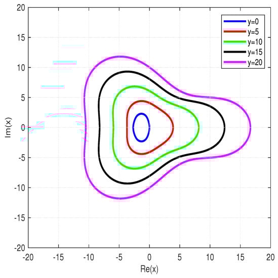
Figure 1. Stability regions of the method.

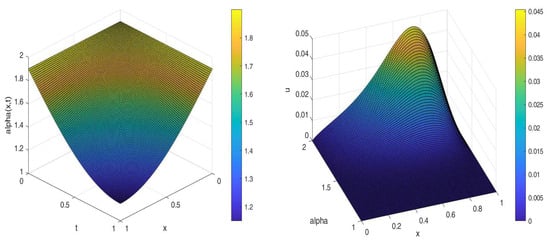
Figure 2. Section 5.1: Graph $\alpha (x,t)$ (left) and solution profile at $t=1$ using $\alpha (x,t)$ (right).

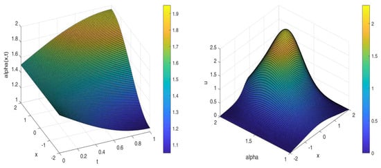
Figure 3. Section 5.3: Graph $\alpha (x,t)$ (left) and solution profile at $t=1$ using $\alpha (x,t)$ (right).

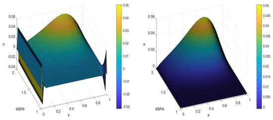
Figure 4. Section 5.1: Graphs of solution profiles using ETD Crank–Nicolson scheme at $t=1$ using $\alpha (x,t)$ with 80 time steps (left) and 160 time steps (right).

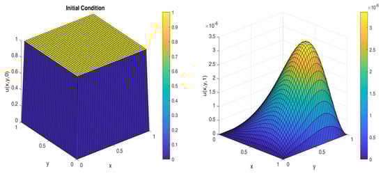
Figure 5. Section 5.2: Initial condition (left) and Solution at $t=1$ using $\alpha (x,t)$ and $\beta (y,t)$ (right).

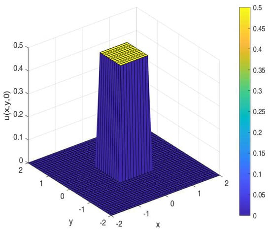
Figure 6. Section 5.4: Graph of the initial conditions.

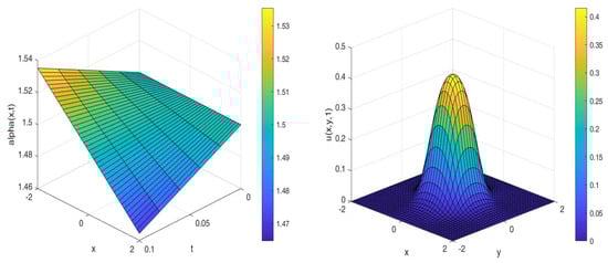
Figure 7. Section 5.4: Graph of $\alpha (x,t)$ for $0\le t\le 0.1$ (left) and solution at $t=0.1$ (right).

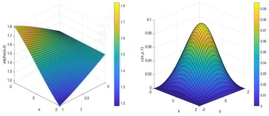
Figure 8. Section 5.4: Graph $\alpha (x,t)$ for $0\le t\le 1$ (left) and the solution at $t=1$ (right).

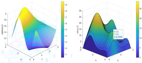
Figure 9. Section 5.4: Graph $\alpha (x,t)$ for $0\le t\le 5$ (left) and solution at $t=5$ (right).

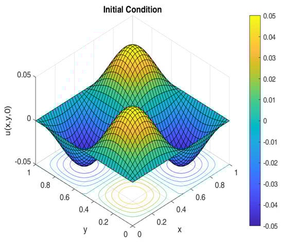
Figure 10. Section 5.5: Graph of the initial conditions.

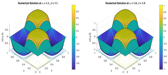
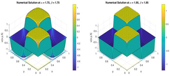
Figure 11. Section 5.5: Graph of the numerical solution of the Allen–Cahn equation at $t=5$ for various values of $\alpha$ and $\beta$.

The superiority of our new scheme over an existing ETD Crank-Nicolson scheme [43] is demonstrated by solving Section 5.1 using both schemes. Third order convergence of our scheme is shown in the Table 1. The second-order convergence of the ETD Crank-Nicolson scheme is shown in Table 2. The ETD Crank-Nicolson scheme is also computationally efficient because it is developed by using the (1, 1)-Padé rational approximation with a single real pole but it is of second-order. Third order convergence of our scheme is also shown in Table 3 by solving Section 5.3.

Table 1. Section 5.1: Convergence results for our time-stepping method.

Time Steps	$\mathit{Error}-{\mathit{L}}_2$	$\mathit{Error}-{\mathit{L}}_{\mathit{\infty }}$	$\mathit{Order}-{\mathit{L}}_2$	$\mathit{Order}-{\mathit{L}}_{\mathit{\infty }}$	CPU Time
20	1.0439 $\times {10}^{-3}$	8.6572 $\times {10}^{-4}$			0.0015
40	2.7328 $\times {10}^{-5}$	1.2955 $\times {10}^{-5}$	2.6555	2.6623	0.0016
80	3.9789 $\times {10}^{-6}$	1.8861 $\times {10}^{-6}$	2.7799	2.7800	0.0019
160	5.4031 $\times {10}^{-7}$	2.5612 $\times {10}^{-7}$	2.8805	2.8805	0.0022
320	7.0630 $\times {10}^{-8}$	3.3480 $\times {10}^{-8}$	2.9354	2.9354	0.0042

Table 2. Section 5.1: Convergence results for the ETD Crank–Nicolson stepping method.

Time Steps	$\mathit{Error}-{\mathit{L}}_2$	$\mathit{Error}-{\mathit{L}}_{\mathit{\infty }}$	$\mathit{Order}-{\mathit{L}}_2$	$\mathit{Order}-{\mathit{L}}_{\mathit{\infty }}$	CPU Time
40	8.1702 $\times {10}^{-5}$	3.8398 $\times {10}^{-5}$	0.0000	0.0000	0.0015
80	2.0658 $\times {10}^{-5}$	9.7932 $\times {10}^{-6}$	1.9837	1.9712	0.0018
160	5.1855 $\times {10}^{-6}$	2.4583 $\times {10}^{-6}$	1.9941	1.9941	0.0019
320	1.2972 $\times {10}^{-6}$	6.1495 $\times {10}^{-7}$	1.9991	1.9991	0.0012
640	3.2428 $\times {10}^{-7}$	1.5373 $\times {10}^{-7}$	2.0001	2.0001	0.0063

Table 3. Section 5.3: Convergence results for the time-stepping method.

Time Steps	$\mathit{Error}-{\mathit{L}}_2$	$\mathit{Error}-{\mathit{L}}_{\mathit{\infty }}$	$\mathit{Order}-{\mathit{L}}_2$	$\mathit{Order}-{\mathit{L}}_{\mathit{\infty }}$	CPU Time
20	2.3984 $\times {10}^{-4}$	9.7746 $\times {10}^{-5}$			0.0015
40	3.7514 $\times {10}^{-5}$	1.5335 $\times {10}^{-5}$	2.6766	2.6722	0.0025
80	5.3142 $\times {10}^{-6}$	2.1845 $\times {10}^{-6}$	2.8195	2.8115	0.0032
160	7.0947 $\times {10}^{-7}$	2.9247 $\times {10}^{-7}$	2.9050	2.9010	0.0043
320	9.2693 $\times {10}^{-8}$	3.8234 $\times {10}^{-8}$	2.9362	2.9353	0.0084

The order of convergence is computed using absolute errors between the consecutive iterations with the following formula:

$$\mathcal{R}={log}_2\frac{\mathcal{E}\left(2k\right)}{\mathcal{E}\left(k\right)},$$

where $\mathcal{E}\left(k\right)=\left|u\right(2k)-u(k\left)\right|$ is the error between consecutive solutions corresponding to time steps $2k$ and k. This approach is used to compute the order of convergence when analytical solutions are not available; see, for example, [35,44]. Convergence errors are computed using the $L_2$ norm and $L_{\infty }$ norm. The computational efficiency of the new method is shown by recording the CPU time for each iteration and is given in the convergence tables. It can be seen that the CPU time is very small even with a large number of time steps. All the calculations are performed using Matlab version R2020b on an Intel Core i7 CPU with 4.0 GHz of speed and 32 GB RAM.

5.1. Space Variable-Order Fractional Enzyme Kinetics Equation in One Dimension

$$\begin{array}{ccc}& & \frac{\partial u}{\partial t}=\frac{{\partial }^{\alpha (x,t)}u}{{\partial \left|x\right|}^{\alpha (x,t)}}-\frac{u}{1+u},0<x<1,t>0,\hfill \\ & & u(x,0)=1,0<x<1,\hfill \\ & & u(0,t)=0,u(1,t)=0,t>0,\hfill \end{array}$$

(42)

$$\begin{array}{ccc}& & \alpha (x,t)=1.95-0.75sin\left(0.5\pi xt\right).\hfill \end{array}$$

(43)

5.2. Space Variable-Order Fractional Enzyme Kinetics Equation in Two Dimensions

$$\begin{array}{ccc}& & \frac{\partial u}{\partial t}=\frac{{\partial }^{\alpha (x,t)}u}{{\partial \left|x\right|}^{\alpha (x,t)}}+\frac{{\partial }^{\beta (y,t)}u}{{\partial \left|y\right|}^{\beta (y,t)}}-\frac{u}{1+u},(x,y)\in \Omega ,t>0,\hfill \\ & & u(x,y,0)=1,(x,y)\in \Omega ,\hfill \\ & & u(x,y,t)=0,(x,y)\in \partial \Omega ,t>0,\hfill \\ & & \alpha (x,t)=1.95-0.75sin\left(0.5\pi xt\right),\beta (y,t)=1.95-0.75sin\left(0.5\pi yt\right),\hfill \end{array}$$

(44)

where $\Omega =[0,1]\times [0,1]$.

5.3. Space Variable-Order Fractional Fisher Equation in One Dimension

$$\begin{array}{ccc}& & \frac{\partial u}{\partial t}=\frac{{\partial }^{\alpha (x,t)}u}{{\partial \left|x\right|}^{\alpha (x,t)}}-u(1-u),-2<x<2,t>0,\hfill \\ & & u(x,0)=\frac{4e^{10x}}{{\left(e^{10x}+1\right)}^2},-2<x<2,\hfill \\ & & u(-2,t)=0,u(2,t)=0,t>0,\hfill \end{array}$$

(45)

$$\begin{array}{ccc}& & \alpha (x,t)=1.5+0.45sin\left(0.25\pi xt\right).\hfill \end{array}$$

(46)

5.4. Space Variable-Order Fractional Fisher Equation in Two Dimensions

$$\begin{array}{ccc}& & \frac{\partial u}{\partial t}=\frac{{\partial }^{\alpha (x,t)}u}{{\partial \left|x\right|}^{\alpha (x,t)}}+\frac{{\partial }^{\beta (y,t)}u}{{\partial \left|y\right|}^{\beta (y,t)}}-u(1-u),(x,y)\in \Omega ,t>0,\hfill \\ & & u(x,y,0)=\left\{\begin{array}{cc}1,& (x,y)\in [-0.5,0.5]\times [-0.5,0.5],\\ 0,& \mathrm{elsewhere},\end{array}\right.\hfill \end{array}$$

(47)

$$\begin{array}{ccc}& & u(x,y,t)=0,(x,y)\in \partial \Omega ,t>0,\hfill \\ & & \alpha (x,t)=1.5-0.45sin\left(0.125\pi xt\right),\beta (y,t)=1.5-0.45sin\left(0.125\pi yt\right),\hfill \end{array}$$

(48)

where $\Omega =[-2,2]\times [-2,2]$.

5.5. Allen–Cahn Equation in Two Dimensions

$$\begin{array}{ccc}& & \frac{\partial u}{\partial t}=\frac{{\partial }^{\alpha }u}{{\partial \left|x\right|}^{\alpha }}+\frac{{\partial }^{\beta }u}{{\partial \left|y\right|}^{\beta }}+u(1-u^2),(x,y)\in \Omega ,t>0,\hfill \end{array}$$

(49)

$$\begin{array}{ccc}& & u(x,y,0)=0.05sin\left(2\pi x\right)sin\left(2\pi y\right)\hfill \end{array}$$

(50)

$$\begin{array}{ccc}& & u(x,y,t)=0,(x,y)\in \partial \Omega ,t>0,\hfill \\ \hfill \end{array}$$

(51)

where $\Omega =[0,1]\times [0,1]$.

6. Conclusions

A novel, highly efficient numerical method has been developed using a single Gaussian quadrature pole rational approximation of the matrix exponential function. An algorithm was constructed based on the method to easily implement the method. Three variable-order fractional–reaction–diffusion problems with nonlinear reaction terms were solved in one and two dimensions. The third-order convergence of the method was proved analytically and verified numerically. Graphs of the solution profiles were plotted to demonstrate the effect of the variable-order diffusion. In the future, we plan to develop similar schemes for systems of reaction–diffusion problems, where several coupled nonlinear equations need to be solved.

References

- Waurick, M. Homogenization in fractional elasticity. SIAM J. Math. Anal. 2014, 46, 1551–1576. [Google Scholar] [CrossRef]
- Luchko, Y.; Punzi, A. Modeling anomalous heat transport in geothermal reservoirs via fractional diffusion equations. GEM-Int. J. Geomath. 2011, 1, 257–276. [Google Scholar] [CrossRef]
- Rida, S.Z.; Yahya, A.A.; Zidan, N.A.; Bakry, H.M. Fractional order of mathematical systems for some bio-chemical application. Fract. Calc. Appl. Anal. 2014, 5, 25. [Google Scholar]
- Maji, S.; Natesan, S. Analytical and numerical solutions of time-fractional advection-diffusion-reaction equation. Appl. Numer. Math. 2023, 185, 549–570. [Google Scholar] [CrossRef]
- Singh, J. Analysis of fractional blood alcohol model with composite fractional derivative. Chaos Solitons Fractals 2020, 140, 110–127. [Google Scholar] [CrossRef]
- Chechkin, A.V.; Gorenflo, R.; Sokolov, I.M. Fractional diffusion in inhomogeneous media. J. Phys. Gen. Phys. 2005, 38, 679–684. [Google Scholar] [CrossRef]
- Sun, H.G.; Chen, W.; Chen, Y. Variable-order fractional differential operators in anomalous diffusion modeling. Phys. A 2009, 388, 4586–4592. [Google Scholar] [CrossRef]
- Zhuang, P.; Liu, F.; Anh, V.; Turner, I. Numerical methods for the variable-order fractional advection-diffusion equation with a nonlinear source term. SIAM J. Numer. Anal. 2009, 47, 1760–1781. [Google Scholar] [CrossRef]
- Diaz, G.; Coimbra, C.F.M. Nonlinear dynamics and control of a variable order oscillator with application to the van der Pol equation. Nonlinear Dynamics 2009, 56, 145–157. [Google Scholar] [CrossRef]
- Kumar, P.; Chaudhary, S.K. Analysis of fractional order control system with performance and stability. International J. Eng. Sci. Technol. 2017, 9, 408–416. [Google Scholar]
- Obembe, A.D.; Hossain, M.E.; Abu-Khamsin, S.A. Variable-order derivative time fractional diffusion model for heterogeneous porous media. J. Pet. Sci. Eng. 2017, 152, 391–405. [Google Scholar] [CrossRef]
- Patnaik, S.; Hollkamp, J.P.; Semperlotti, F. Applications of variable-order fractional operator—A review. Proc. R. Soc. 2020, 476, 20190498. [Google Scholar] [CrossRef] [PubMed]
- Li, C.P.; Zeng, F.H. Numerical Methods for Fractional Differential Calculus; Chapman and Hall/CRC: Boca Raton, FL, USA, 2015. [Google Scholar]
- Li, C.P.; Cai, M. Theory and Numerical Approximations of Fractional Integrals and Derivatives; SIAM Philadelphia: Philadelphia, PA, USA, 2019. [Google Scholar]
- Glockle, W.G.; Nonnenmacher, T.F. A fractional calculus approach to self-similar protein dynamics. Biophys. J. 1995, 68, 46–53. [Google Scholar] [CrossRef] [PubMed]
- Klass, D.L.; Martinek, T.W. Electroviscous fluids. I. Rheological Properties. J. Appl. Phys. 1967, 38, 67–74. [Google Scholar] [CrossRef]
- Shiga, T. Deformation and viscoelastic behavior of polymer gel in electric fields. Proc. Jpn. Acad. Ser. Phys. Biol. Sci. 1998, 74, 6–11. [Google Scholar] [CrossRef]
- Davis, L.C. Model of Magnetorheological Elastomers. J. Appl. Phys. 1999, 85, 3342–3351. [Google Scholar] [CrossRef]
- Samko, S.G.; Ross, B. Integration and differentiation to a variable fractional order. Integral Transform. Spec. Funct. 1993, 1, 277–300. [Google Scholar] [CrossRef]
- Lin, R.; Liu, F.; Anh, V.; Turner, I. Stability and convergence of a new explicit finite difference approximation for the variable-order nonlinear fractional diffusion equation. Appl. Math. Comput. 2009, 2, 435–445. [Google Scholar] [CrossRef]
- Sun, H.; Chen, W.; Li, C.P.; Chen, Y. Finite difference schemes for variable order time fractional diffusion equation. Int. J. Bifurc. Chaos 2012, 22, 1250085. [Google Scholar] [CrossRef]
- Kheirkhah, F.; Hajipour, M.; Baleanu, D. The performance of a numerical scheme on the variable-order time-fractional advection-reaction-subdiffusion equations. Appl. Numer. Math. 2022, 178, 25–40. [Google Scholar] [CrossRef]
- Heydari, M.H.; Avazzadeh, Z.; Razzaghi, M. Vieta-Lucas polynomials for the coupled nonlinear variable-order fractional Ginzburg-Landau equations. Appl. Numer. Math. 2021, 165, 442–458. [Google Scholar] [CrossRef]
- Yan, R.; Ma, Q.; Ding, X. Convergence analysis of the hp-version spectral collocation method for a class of nonlinear variable-order fractional differential equations. Appl. Numer. Math. 2021, 170, 269–297. [Google Scholar] [CrossRef]
- Darve, E.; Delia, M.; Garrappa, R.; Giusti, A.; Rubio, N.L. On the fractional Laplacian of variable order. Fract. Calc. Appl. Anal. 2022, 25, 15–28. [Google Scholar] [CrossRef]
- Garrappa, R.; Giusti, A.; Mainardi, F. Variable-order fractional calculu. A change of perspective. Commun. Nonlinear Sci. Numer. Simul. 2021, 102, 105904. [Google Scholar] [CrossRef]
- Xu, Y.; Sun, H.; Zhang, Y.; Sun, H.W. A novel meshless method based on RBF for solving variable-order time fractional advection-diffusion-reaction equation in linear or nonlinear systems Image. Comput. Math. Appl. 2023, 142, 107–120. [Google Scholar] [CrossRef]
- Li, X.Y.; Wu, B.Y. Iterative reproducing kernel method for nonlinear variable-order space fractional diffusion equations. Int. J. Comput. Math. 2018, 95, 1210–1221. [Google Scholar]
- Sun, H.; Chang, A.; Zhang, Y.; Chen, W. A review on variable-order fractional differential equation. Mathematical foundations, physical models, and its applications. Fract. Calc. Appl. Anal. 2019, 22, 27–59. [Google Scholar] [CrossRef]
- Khaliq, A.Q.M.; Liang, X.; Furati, K.M. A fourth-order implicit-explicit scheme for the space fractional nonlinear Schrödinger equations. Numer. Algorithms 2017, 75, 147–172. [Google Scholar] [CrossRef]
- Ngo, H.T.B.; Razzaghi, M.; Vo, T.N. Fractional order Chelyshkov wavelet method for solving variable order fractional differential equations and an application in variable order fractional relaxation system. Numer. Algor. 2023, 92, 1571–1588. [Google Scholar] [CrossRef]
- Ding, H.F. The construction of an optimal fourth-order fractional-compact-type numerical differential formula of the Riesz derivative and its application. Commun. Nonlinear Sci. Numer. Simul. 2023, 23, 107272. [Google Scholar] [CrossRef]
- Ding, H.F.; Li, C.P. High order numerical algorithm and error analysis for the two-dimensional nonlinear spatial fractional complex Ginzburg-Landau equation. Commun. Nonlinear Sci. Numer. Simul. 2023, 120, 107160. [Google Scholar] [CrossRef]
- Furati, K.M.; Yousuf, M.; Khaliq, A.Q.M. Fourth-order methods for space fractional reaction-diffusion equations with non-smooth data. Int. J. Comput. Math. 2018, 95, 1240–1256. [Google Scholar] [CrossRef]
- Yousuf, M.; Furati, K.M.; Khaliq, A.Q.M. High-order time-stepping methods for two-dimensional Riesz fractional nonlinear reaction-diffusion equations. Comput. Math. Appl. 2020, 80, 204–226. [Google Scholar] [CrossRef]
- Wang, Q.Y.; She, Z.H.; Lao, C.X.; Lin, F.R. Fractional centered difference schemes and banded preconditioners for nonlinear Riesz space variable-order fractional diffusion equations. Numer. Algor. 2023. [Google Scholar] [CrossRef]
- Thomee, V. Galerkin Finite Element Methods for Parabolic Problems; Series in Computational Mathematics; Springer: Berlin/Heidelberg, Germany, 2006. [Google Scholar]
- Ortigueira, M.D. Riesz potential operators and inverses via fractional centered derivatives. Int. J. Math. Math. Sci. 2006, 2006, 48391. [Google Scholar] [CrossRef]
- Celik, C.; Duman, M. Crank-Nicolson method for the fractional diffusion equation with the Riesz fractional derivative. J. Comput. Phys. 2012, 231, 1743–1750. [Google Scholar] [CrossRef]
- Pazy, A. Semigroups of Linear Operators and Applications to Partial Differential Equations; Springer: Berlin/Heidelberg, Germany, 1983. [Google Scholar]
- Norsett, S.P.; Wolfbrandt, A. Attainable order of rational approximations to the exponential function with only real poles. Bit Numer. Math. 1977, 17, 200–208. [Google Scholar] [CrossRef]
- Cox, S.M.; Matthews, P.C. Exponential Time Differencing for Stiff Systems. J. Comput. Phys. 2002, 176, 430–455. [Google Scholar] [CrossRef]
- Kleefeld, B.; Khaliq, A.Q.M.; Wade, B.A. An ETD Crank-Nicolson method for reaction-diffusion systems. Numer. Methods Partial. Differ. Eq. 2012, 28, 1309–1335. [Google Scholar] [CrossRef]
- Pooley, D.M.; Vetzal, K.R.; Forsyth, P.A. Convergence Remedies for Non- Smooth Payoffs in Option Pricing. J. Comput. Financ. 2003, 6, 25–40. [Google Scholar] [CrossRef]
Disclaimer/Publisher’s Note: The statements, opinions and data contained in all publications are solely those of the individual author(s) and contributor(s) and not of MDPI and/or the editor(s). MDPI and/or the editor(s) disclaim responsibility for any injury to people or property resulting from any ideas, methods, instructions or products referred to in the content. |
© 2023 by the authors. Licensee MDPI, Basel, Switzerland. This article is an open access article distributed under the terms and conditions of the Creative Commons Attribution (CC BY) license (https://creativecommons.org/licenses/by/4.0/).