A Fast θ Scheme Combined with the Legendre Spectral Method for Solving a Fractional Klein–Gordon Equation

Abstract

In the current work, a fast $\theta$ scheme combined with the Legendre spectral method was developed for solving a fractional Klein–Gordon equation (FKGE). The numerical scheme was provided by the Legendre spectral method in the spatial direction, and for the temporal direction, a $\theta$ scheme of order $O\left({\tau }^2\right)$ with a fast algorithm was taken into account. The fast algorithm could decrease the computational cost from $O\left(M^2\right)$ to $O(MlogM)$, where M denotes the number of time levels. In addition, correction terms could be employed to improve the convergence rate when the solutions have weak regularity. We proved theoretically that the scheme is unconditionally stable and obtained an error estimate. The numerical experiments demonstrated that our numerical scheme is accurate and efficient.

1. Introduction

Fractional differential equations (FDEs), as the evolution of integral differential equations, can more precisely describe phenomena with sophisticated dynamics [1,2,3,4]. In the past few decades, FDEs have been investigated by a number of scholars because they have practical applications in various fields, such as relativistic quantum mechanics [5], hydromechanics [6], neuroscience [7], and materials science [8]. Due to it being virtually impossible to obtain an analytic solution to an FDE in most cases, many numerical methods for solving FDEs have been developed rapidly. In particular, finite difference methods (FDMs) [9,10], finite element methods (FEMs) [11,12,13], spectral methods [14,15,16], and spectral element methods [17,18] have been extensively utilized.

In this article, we concentrate on the following FKGE:

$$\left\{\begin{array}{cc}\frac{{\partial }^{\alpha }\xi (x,t)}{\partial t^{\alpha }}+\rho \frac{\partial \xi (x,t)}{\partial t}+\xi (x,t)=\frac{{\partial }^2\xi (x,t)}{\partial x^2}+f(x,t),\hfill & x\in (0,L),t\in (0,T]\hfill \\ \xi (x,0)=\varphi \left(x\right),\frac{\partial \xi (x,0)}{\partial t}=\phi \left(x\right),\hfill & x\in (0,L),\hfill \\ \xi (0,t)=0,\xi (L,t)=0,\hfill & t\in [0,T],\hfill \end{array}\right.$$

(1)

When $\alpha =2$, (1) is a classical integer-order Klein–Gordon equation. $D_{0,t}^{\alpha }\xi \left(t\right)$ is a fractional derivative with respect to t in the Caputo sense, which is defined as

$$D_{0,t}^{\alpha }\xi (x,t)=\frac{{\partial }^{\alpha }\xi \left(x\right)}{\partial t^{\alpha }}=\left\{\begin{array}{ccc}\frac{1}{\mathsf{\Gamma }(2-\alpha )}{\int }_0^t\frac{{\partial }^2\xi (x,s)}{\partial s^2}\frac{\mathrm{d}s}{{(t-s)}^{1-\alpha }},\hfill & \hfill & 1<\alpha <2\hfill \\ \frac{{\partial }^2\xi \left(x\right)}{\partial t^2}.\hfill & \hfill & \alpha =2\hfill \end{array}\right.$$

If we set $\rho =0$, then an FKGE can be obtained, and a fractional dissipative Klein–Gordon equation can be obtained for $\rho >0$ [19].

The application of FDEs has been extended to quantum mechanics, which has given rise to fractional quantum mechanics [20,21]. Klein–Gordon equations, which are some of the most fundamental equations in relativistic quantum mechanics, have been generalized to FKGEs [19,22]. As a matter of fact, quite a few scholars have investigated FKGEs. Vong et al. proposed a high-order finite difference scheme for a nonlinear FKGE, and the convergence order of the proposed scheme was $O(h^4+{\tau }^{3-\alpha })$ [23], where h and $\tau$ are the spatial and temporal step sizes, respectively. Hashemizadeh et al. proposed an approach that relied on the sparse operational matrix of the derivative to solve an FKGE, leading to more efficient operation [19]. By combining the properties of Chebyshev approximations with the FDM, Khadera et al. developed a method that reduced an FKGE to a system of ODEs and then solved it using the FDM [24]. Recently, Saffarian et al. utilized the ADI spectral element method to solve a nonlinear FKGE with a convergent order of $O({\tau }^2+N^{1-m}$) [25], where N is the polynomial degree and m represents the regularity of the solution. As far as the authors’ knowledge is concerned, there have been few reports on numerical methods utilizing fast algorithms for an FKGE. Motivated by the above considerations, our main aim was developing a stable and fast numerical method for FKGEs.

The structure of this paper is as follows: In Section 2, some crucial preliminaries are provided for the subsequent analysis. In Section 3, to obtain the fully discrete scheme, we introduce the $\theta$ scheme and the Legendre spectral method in the temporal and spatial directions, respectively. Meanwhile, correction terms are considered to improve the weak regularity of the solution. In Section 4, we attach importance to the stability analysis and the convergence analysis. To save on computational expenses for the fractional operators, a fast algorithm is implemented in Section 5. In Section 6, several numerical experiments are conducted to validate our theoretical analysis. In the final section, we present our conclusions.

2. Preliminaries

In this section, some lemmas and definitions that were necessary for the following analysis are presented.

The space $P_N\left(\mathsf{\Omega }\right)$ corresponds to the set of polynomials defined in the domain $\mathsf{\Omega }$, encompassing polynomials with a degree lower than N. Moreover, within $P_N\left(\mathsf{\Omega }\right)$, we have the subspace $P_N^0\left(\mathsf{\Omega }\right)$ that fulfills the boundary condition $w\left(\partial \mathsf{\Omega }\right)=0$ for $w\in P_N\left(\mathsf{\Omega }\right).$

Let us denote ${\pi }_N^{1,0}\left(\mathsf{\Omega }\right)$ as the orthogonal projection operator from the Hilbert space $H_0^1\left(\mathsf{\Omega }\right)$ to the subspace $P_N^0$. For any $w\in H_0^1\left(\mathsf{\Omega }\right)$ and any $v\in P_N^0\left(\mathsf{\Omega }\right)$, the orthogonal projection operator ${\pi }_N^{1,0}\left(\mathsf{\Omega }\right)$ exhibits the following property:

$$\begin{array}{c}\hfill ({\partial }_x{\pi }_N^{1,0}w,{\partial }_x\upsilon )=({\partial }_{x}w,{\partial }_x\upsilon ).\end{array}$$

Here, we make a crucial assumption that the solution to Equation (1) conforms to the following form [11,17]:

$$\xi (x,t)=\varphi +\phi t+c_2{t}^{{\sigma }_2}+c_3{t}^{{\sigma }_3}+\cdots =\varphi +\phi t+\sum _{k=2}^n{c}_j{t}^{{\sigma }_k}+\mathsf{\Phi }(x,t),$$

(2)

where ${\sigma }_1=1$; ${\sigma }_k<{\sigma }_{k+1},k\le n-1$; $c_k\in H_0^1\left(\mathsf{\Omega }\right)\cap H^n\left(\mathsf{\Omega }\right);$ and $\mathsf{\Phi }(x,t)$ is a function that is sufficiently smooth with respect to both variables x and t. There exists $c_k\ne 0$ for $k=2,3,\cdots ,n.$

We define $\sigma$ as:

$$\sigma =\left\{\begin{array}{ccc}{\sigma }_2,\hfill & \hfill & \phi =0\hfill \\ 1,\hfill & \hfill & \mathrm{otherwise}\hfill \end{array}\right.$$

(3)

which describes the regularity of (2).

Lemma 1

([14,16]). Suppose $\xi \in H_0^1\left(\mathsf{\Omega }\right)\cap H^m\left(\mathsf{\Omega }\right)$; then, we have

$$\begin{array}{c}\hfill \left|\right|\xi -{\pi }_N^{1,0}\xi \left|\right|\le C{N}^{-m}\left|\right|\xi \left|\right|.\end{array}$$

(4)

Lemma 2

([11,19]). Let $\xi \left(t\right)$ be a continuous function with a fractional derivative of order α; then, we have

$$I_{0,t}^{\alpha }{D}_{0,t}^{\alpha }\xi \left(t\right)=\xi \left(t\right)-\sum _{i=0}^{n-1}{\xi }^{\left(k\right)}\frac{t^k}{k!},n-1<\alpha \le n,n\in N.$$

(5)

Lemma 3

([11]). Suppose $\xi \left(t\right)\in C^k[0,T]$ for $k\in {\mathbb{N}}^{+}$. Let $ϵ,\gamma >0$ with $l\le k$ and $\gamma ,\gamma +ϵ\in [l-1,l]$. Then, we have

$$D_{0,t}^{ϵ}{D}_{0,t}^{\gamma }\xi =D^{ϵ+\gamma }\xi .$$

(6)

Integrating both sides of (1) with the operator $I_{0,t}^{\alpha -1}$ and combining Lemmas 2 and 3, we obtain

$${\xi }_t+\rho D_{0,t}^{2-\alpha }\xi +I_{0,t}^{\alpha -1}\xi =I_{0,t}^{\alpha -1}\Delta \xi +\phi +\rho {\left[D_{0,t}^{2-\alpha }\xi \right]}_{t=0}+F(x,t),$$

(7)

where $F(x,t)=I_{0,t}^{\alpha -1}f(x,t).$ Under the assumption of (2), $\rho {\left[D_{0,t}^{2-\alpha }\xi \right]}_{t=0}=0$.

3. Fully Discrete Scheme

Let $\tau$ be a temporal step size and $t_n=n\tau (0\le n\le M),M=[1/\tau ].$${\xi }^k\triangleq \xi \left(t_k\right)=\xi \left(k\tau \right).$ For the discretization of fractional operators ($\eta \in (0,1)$) and the first-order derivative, we utilize the $\theta$ schemes as follows [11,12]:

$$\begin{array}{cc}\hfill & D_{0,t}^{\eta }\xi \left(t_{n-\theta }\right)=D_{\tau ,\eta }^{n,\theta }u+E_{n-\theta }^{\left(1\right)}={\tau }^{-\eta }\sum _{k=0}^n{\omega }_{n-k}^{\left(\eta \right)}({\xi }^k-{\xi }^0)+E_{n-\theta }^{\left(1\right)},\hfill \\ \hfill & I_{0,t}^{\eta }\xi \left(t_{n-\theta }\right)=I_{\tau ,\eta }^{n,\theta }u+E_{N-\theta }^{\left(2\right)}={\tau }^{\eta }\sum _{k=0}^n{\omega }_{n-k}^{(-\eta )}({\xi }^k-{\xi }^0)+I_{0,t_{n-\theta }}^{\left(\eta \right)}+E_{n-\theta }^{\left(2\right)},\hfill \\ \hfill & {\xi }_t\left(t_{n-\theta }\right)={\xi }_{\tau ,\theta }^n+E_{n-\theta }^{\left(3\right)}\hfill \\ \hfill & =\left\{\begin{array}{ccc}\frac{{\xi }^1-{\xi }^0}{\tau }+E_{1-\theta }^{\left(1\right)},\hfill & \hfill & n=1\hfill \\ \frac{3-2\theta }{2\tau }{\xi }^n-\frac{2-2\theta }{\tau }{\xi }^{n-1}+\frac{1-2\theta }{2\tau }{\xi }^{n-2}+E_{n-\theta }^{\left(3\right)},\hfill & \hfill & n\ge 2\hfill \end{array}\right.\hfill \end{array}$$

(8)

where $E_{n-\theta }^{\left(1\right)}=O\left(t_{n-\theta }^{\sigma -\eta -2}{\tau }^2\right),E_{n-\theta }^{\left(2\right)}=O\left(t_{n-\theta }^{\sigma +\eta -2}{\tau }^2\right)$, $E_{n-\theta }^{\left(3\right)}=O\left(t_{n-\theta }^{\overline{\sigma }-3}{\tau }^2\right),$ $\overline{\sigma }=min\{{\sigma }_2,{\sigma }_3,\cdots \}$. The following expression captures the relationship between the generating function $\omega (\xi ,\delta )$ and its expansion coefficients ${\omega }_k^{\left(\delta \right)}$:

$$\begin{array}{c}\hfill \omega (\xi ,\delta )=\sum _{k=0}^{\infty }{\omega }_k^{\left(\delta \right)}{\xi }^k=\frac{{(1-\xi )}^{\delta }}{1-(\frac{\delta }{2}-\theta )(1-\xi )},\delta \in (-1,0)\cup (0,1),\end{array}$$

where $\theta \in (\frac{\delta -1}{2},1]$, and the choice of $\theta$ does not affect the convergence rate. When $\theta =\frac{\alpha }{2}$, it simplifies to a fractional Crank–Nicolson scheme [26]. We apply the following formula to determine expansion coefficients ${\omega }_k^{\left(\delta \right)}$:

$${\omega }_k^{\left(\delta \right)}=\left\{\begin{array}{ccc}2/\left[2\right(1+\theta )-\delta ],\hfill & \hfill & k=0\hfill \\ 4V_1^1/{[2(1+\theta )-\delta ]}^2,\hfill & \hfill & k=1\hfill \\ (V_k^1{\omega }_{k-1}^{\left(\delta \right)}+V_k^2{\omega }_{k-2}^{\left(\delta \right)})/(1+\theta -\delta /2)/k,\hfill & \hfill & k\ge 2\hfill \end{array}\right.$$

(9)

where

$$\begin{array}{cc}\hfill & V_k^1=\frac{{\delta }^2}{2}-(\theta +k+\frac{1}{2})\delta +k\theta +k-1,\hfill \\ \hfill & V_k^2=-\frac{{\delta }^2}{2}+(\theta +\frac{k-1}{2})\delta +(1-k)\theta .\hfill \end{array}$$

The semi-discrete scheme of (7) is obtained in the temporal direction utilizing (8) as follows:

$${\xi }_{\tau ,\theta }^n+\rho D_{\tau ,2-\alpha }^{n,\theta }\xi +I_{\tau ,\alpha -1}^{n,\theta }\xi =I_{\tau ,\alpha -1}^{n,\theta }\Delta \xi +\phi +F^{n-\theta }+E_{n-\theta },$$

(10)

where $F^{n-\theta }=F(x,t_{n-\theta })$, and $E_{n-\theta }$ is

$$E_{n-\theta }=O\left(t_{n-\theta }^{\sigma +\alpha -4}{\tau }^2\right)+O\left(t_{n-\theta }^{\tilde{\sigma }-3}{\tau }^2\right).$$

(11)

The Legendre spectral method is applied for the discretization in the spatial direction and used to find $Z\in P_N^0\left(\mathsf{\Omega }\right)$ for $\forall \zeta \in P_N^0\left(\mathsf{\Omega }\right)$, such that

$$\begin{array}{cc}\hfill & (Z_{\tau ,\theta }^n,\zeta )+(\rho D_{\tau ,2-\alpha }^{n,\theta }Z,\zeta )+(I_{\tau ,\alpha -1}^{n,\theta }Z,\zeta )=(I_{\tau ,\alpha -1}^{n,\theta }\Delta Z,\zeta )+(\phi ,\zeta )+(F^{n-\theta },\zeta ),\hfill \\ & \mathrm{with}{Z}^0={\pi }_N^{1,0}{\xi }^0.\hfill \end{array}$$

(12)

We see from the truncation errors in (8) that if $\sigma <3$, then the convergence order in the temporal direction is lower than $O\left({\tau }^2\right)$. Generally, the solutions of FKGEs have weak regularity. To improve the convergence rate, correction terms are added to the approximation formulas as follows [17,27,28]:

$$\left\{\begin{array}{c}{D}_{0,t}^{\delta }\xi \left(t_{n-\theta }\right)\approx D_{\tau ,\delta }^{n,\theta }\xi +{\tau }^{-\delta }\sum _{j=1}^m{w}_{n,j}^{\left(\delta \right)}({\xi }^j-{\xi }^0),\hfill \\ I_{0,t}^{\delta }\xi \left(t_{n-\theta }\right)\approx I_{\tau ,\delta }^{n,\theta }\xi +{\tau }^{\delta }\sum _{j=1}^m{w}_{n,j}^{(-\delta )}({\xi }^j-{\xi }^0),\hfill \\ {\xi }_t\left(t_{n-\theta }\right)\approx {\xi }_{\tau ,\theta }^n+{\tau }^{-1}\sum _{j=1}^m{w}_{n,j}^{\left(1\right)}({\xi }^j-{\xi }^0),\hfill \end{array}\right.$$

(13)

where $w_{n,j}^{\left(\delta \right)}$, $w_{n,j}^{(-\delta )}$, and $w_{n,j}^{\left(1\right)}$ are starting weights, and they can be derived by solving a linear system of equations. Take an example for calculating $w_{n,j}^{(-\delta )}$ in (13). $I_{0,t}^{\delta }\xi \left(t_{n-\theta }\right)=I_{\tau ,\delta }^{n,\theta }\xi +{\tau }^{\delta }{\sum }_{j=1}^m{w}_{n,j}^{(-\delta )}({\xi }^j-{\xi }^0)$ is exact for $\xi \left(t\right)=t^{{\sigma }_r}({\sigma }_r<2-\delta )$. Then, it can be solved through the following linear system:

$$\sum _{j=1}^m{w}_{n,j}^{(-\delta )}{t}_j^{{\sigma }_r}={\tau }^{-\delta }\frac{\mathsf{\Gamma }({\sigma }_r+1)}{\mathsf{\Gamma }({\sigma }_r+1+\delta )}{t}_{n-\theta }^{{\sigma }_r+\delta }-\sum _{k=1}^n{\omega }_{n-k}^{(-\delta )}{t}_k^{{\sigma }_r}.$$

(14)

4. Stability and Convergence Analysis

Lemma 4

([11]). For any vector $({\xi }^1,..,{\xi }^M)\in {\mathbb{R}}^M$ with $M\ge 1$, ${\omega }_k^{\left(\delta \right)}$ is defined in (8) ($\delta \in (-1,0)\cup (0,1)$) and $\theta \in (\frac{\delta -1}{2},1]$. Thus, we have

$$\sum _{k=1}^M\sum _{i=1}^k{\omega }_{k-i}^{\left(\delta \right)}{\xi }^i{\xi }^k\ge 0.$$

(15)

Lemma 5

([11]). For any vector $({\xi }^1,...,{\xi }^M)\in {\mathbb{R}}^M$ with $M\ge 2$, ${\xi }^0=0$ and ${\xi }_{\tau ,\theta }^j$ are defined in (8), and we have

$$\sum _{j=1}^M{\xi }^j{\xi }_{\tau ,\theta }^j\ge \frac{1}{4\tau }{\left({\xi }^M\right)}^2-\frac{1}{2\tau }{\left({\xi }^1\right)}^2$$

(16)

with $\theta \in [0,1].$

Theorem 1.

The scheme in (12) is unconditionally stable, and we have the following estimate:

$$\begin{array}{c}\hfill \left|\right|Z^M\left|\right|\le C\left(\right|\left|\varphi \right||+\left|\right|▵\varphi \left|\right|+\left|\right|\phi \left|\right|+\underset{0\le j\le M}{max}\left|\right|F^j\left|\right|).\end{array}$$

(17)

Proof. 

$Z^0$ is the proper approximation of $\varphi$ that satisfies $\left|\right|Z^0\left|\right|\le \left|\right|\varphi \left|\right|$ and $\left|\right|\nabla Z^0\left|\right|\le \left|\right|\nabla \varphi \left|\right|$. Defining ${\mathsf{\Lambda }}^n\triangleq Z^n-Z^0$ and considering (8), we can obtain

$$\begin{array}{c}{Z}_{\tau ,\theta }^n={\mathsf{\Lambda }}_{\tau ,\theta }^n,\hfill \\ D_{\tau ,\alpha }^{n,\theta }Z=D_{\tau ,\alpha }^{n,\theta }\mathsf{\Lambda },\hfill \\ I_{\tau ,\alpha }^{n,\theta }Z=I_{\tau ,\alpha }^{n,\theta }\mathsf{\Lambda }+I_{0,t_{n-\theta }}^{\alpha }{Z}^0,\hfill \\ I_{\tau ,\alpha }^{n,\theta }\nabla Z=I_{\tau ,\alpha }^{n,\theta }\nabla \mathsf{\Lambda }+I_{0,t_{n-\theta }}^{\alpha }\nabla Z^0.\hfill \end{array}$$

(18)

Replacing $\zeta$ with ${\mathsf{\Lambda }}^n$ in (12) and using (18), we obtain

$$\begin{array}{c}({\mathsf{\Lambda }}_{\tau ,\theta }^n,{\mathsf{\Lambda }}^n)+(\rho D_{\tau ,2-\alpha }^{n,\theta }\mathsf{\Lambda },{\mathsf{\Lambda }}^n)+(I_{\tau ,\alpha -1}^{n,\theta }\mathsf{\Lambda },{\mathsf{\Lambda }}^n)+(I_{\tau ,\alpha -1}^{n,\theta }\nabla \mathsf{\Lambda },\nabla {\mathsf{\Lambda }}^n)\hfill \\ =(\phi ,{\mathsf{\Lambda }}^n)+(F^{n-\theta },{\mathsf{\Lambda }}^n)-(I_{0,t_{n-\theta }}^{\alpha -1}{Z}^0,{\mathsf{\Lambda }}^n)-(I_{0,t_{n-\theta }}^{\alpha -1}\nabla Z^0,\nabla {\mathsf{\Lambda }}^n).\hfill \end{array}$$

(19)

By substituting n with j and taking the summation of both sides for j ranging from 1 to M (M $\ge 2$), we can derive

$$\begin{array}{c}\sum _{j=1}^M({\mathsf{\Lambda }}_{\tau ,\theta }^j,{\mathsf{\Lambda }}^j)+\sum _{j=1}^M(\rho D_{\tau ,2-\alpha }^{j,\theta }\mathsf{\Lambda },{\mathsf{\Lambda }}^j)+\sum _{j=1}^M(I_{\tau ,\alpha -1}^{j,\theta }\mathsf{\Lambda },{\mathsf{\Lambda }}^j)+\sum _{j=1}^M(I_{\tau ,\alpha -1}^{j,\theta }\nabla \mathsf{\Lambda },\nabla {\mathsf{\Lambda }}^j)\hfill \\ =\sum _{j=1}^M(\phi ,{\mathsf{\Lambda }}^j)+\sum _{j=1}^M(F^{j-\theta },{\mathsf{\Lambda }}^j)-\sum _{j=1}^M(I_{0,t_{j-\theta }}^{\alpha -1}{Z}^0,{\mathsf{\Lambda }}^j)-\sum _{j=1}^M(I_{0,t_{j-\theta }}^{\alpha -1}\nabla Z^0,\nabla {\mathsf{\Lambda }}^j).\hfill \end{array}$$

(20)

Combining Lemmas 4 and 5, we derive the following inequality:

$$\begin{array}{c}\sum _{j=1}^M({\mathsf{\Lambda }}_{\tau ,\theta }^j,{\mathsf{\Lambda }}^j)\ge \frac{1}{4\tau }\left|\right|{\mathsf{\Lambda }}^M{\left|\right|}^2-\frac{1}{2\tau }\left|\right|{\mathsf{\Lambda }}^1{\left|\right|}^2,\hfill \\ \sum _{j=1}^M(\rho D_{\tau ,2-\alpha }^{j,\theta }\mathsf{\Lambda },{\mathsf{\Lambda }}^j)={\tau }^{\alpha -2}{\int }_0^1\rho \sum _{j=1}^M{\mathsf{\Lambda }}^j\sum _{k=1}^j{\omega }_{j-k}^{(2-\alpha )}{\mathsf{\Lambda }}^{k}dx\ge 0,\hfill \\ \sum _{j=1}^M(I_{\tau ,\alpha -1}^{j,\theta }\mathsf{\Lambda },{\mathsf{\Lambda }}^j)={\tau }^{\alpha -1}{\int }_0^1\sum _{j=1}^M{\mathsf{\Lambda }}^j\sum _{k=1}^j{\omega }_{j-k}^{(1-\alpha )}{\mathsf{\Lambda }}^{k}dx\ge 0,\hfill \\ \sum _{j=1}^M(I_{\tau ,\alpha -1}^{j,\theta }\nabla \mathsf{\Lambda },\nabla {\mathsf{\Lambda }}^j)={\tau }^{\alpha -1}{\int }_0^1\sum _{j=1}^M\nabla {\mathsf{\Lambda }}^j\sum _{k=1}^j{\omega }_{j-k}^{(1-\alpha )}\nabla {\mathsf{\Lambda }}^{k}dx\ge 0,\hfill \end{array}$$

(21)

$$\sum _{j=1}^M(\phi ,{\mathsf{\Lambda }}^j)\le \frac{1}{2}\sum _{j=1}^M{\left(\right|\left|\phi \right||}^2+\left|\right|{\mathsf{\Lambda }}^j{\left|\right|}^2)=\frac{M}{2}{\left|\right|\phi \left|\right|}^2+\frac{1}{2}\sum _{j=1}^M\left|\right|{\mathsf{\Lambda }}^j{\left|\right|}^2,$$

(22)

$$\begin{array}{cc}\hfill \sum _{j=1}^M(F^{j-\theta },{\mathsf{\Lambda }}^j)\le & \frac{1}{2}\sum _{j=1}^M(||F^{j-\theta }{\left|\right|}^2+\left|\right|{\mathsf{\Lambda }}^j{\left|\right|}^2)\hfill \\ \hfill \le & \frac{1}{2}\sum _{j=1}^M\left|\right|{\mathsf{\Lambda }}^j{\left|\right|}^2+C\sum _{j=1}^M(||F^j{\left|\right|}^2+\left|\right|F^{j-1}{\left|\right|}^2)\hfill \\ \hfill \le & \frac{1}{2}\sum _{j=1}^M\left|\right|{\mathsf{\Lambda }}^j{\left|\right|}^2+C\sum _{j=0}^M\left|\right|F^j{\left|\right|}^2,\hfill \end{array}$$

(23)

$$\begin{array}{cc}\hfill \sum _{j=1}^M(I_{0,t_{j-\theta }}^{\alpha -1}{Z}^0,{\mathsf{\Lambda }}^j)& =\sum _{j=1}^M\left(I_{0,t_{j-\theta }}^{\alpha -1}1\right)(Z^0,{\mathsf{\Lambda }}^j)\le \frac{1}{\mathsf{\Gamma }\left(\alpha \right)}\sum _{j=1}^M\left|(Z^0,{\mathsf{\Lambda }}^j)\right|\hfill \\ & \le \frac{M}{2\mathsf{\Gamma }\left(\alpha \right)}\left|\right|Z^0{\left|\right|}^2+\frac{1}{2\mathsf{\Gamma }\left(\alpha \right)}\sum _{j=1}^M\left|\right|{\mathsf{\Lambda }}^j{\left|\right|}^2\hfill \\ & \le \frac{M}{2\mathsf{\Gamma }\left(\alpha \right)}{\left|\right|\varphi \left|\right|}^2+\frac{1}{2\mathsf{\Gamma }\left(\alpha \right)}\sum _{j=1}^M\left|\right|{\mathsf{\Lambda }}^j{\left|\right|}^2.\hfill \end{array}$$

(24)

Let ${\Delta }_N$ be the operator from $P_N^0$ into $P_N^0$, such that

$$({\Delta }_N\Psi ,\upsilon )=-(\nabla \Psi ,\nabla \upsilon ),\forall \Psi ,\upsilon \in P_N^0.$$

(25)

For a properly defined $Z^0$, it holds that $\left|\right|{\Delta }_N{Z}^0\left|\right|\le \left|\right|\Delta \varphi \left|\right|;$ thus, we have the following inequality:

$$\begin{array}{cc}\hfill -\sum _{j=1}^M(I_{0,t_{j-\theta }}^{\alpha -1}\nabla Z^0,\nabla {\mathsf{\Lambda }}^j)& =\sum _{j=1}^M\frac{t_{j-\theta }^{\alpha -1}}{\mathsf{\Gamma }\left(\alpha \right)}({\Delta }_N{Z}^0,{\mathsf{\Lambda }}^j)\le \frac{1}{\mathsf{\Gamma }\left(\alpha \right)}\sum _{j=1}^M({\Delta }_N{Z}^0,{\mathsf{\Lambda }}^j)\hfill \\ & \le \frac{M}{2\mathsf{\Gamma }\left(\alpha \right)}\left|\right|{\Delta }_N{Z}^0{\left|\right|}^2+\frac{1}{2\mathsf{\Gamma }\left(\alpha \right)}\sum _{j=1}^M\left|\right|{\mathsf{\Lambda }}^j{\left|\right|}^2\hfill \\ & \le \frac{M}{2\mathsf{\Gamma }\left(\alpha \right)}{\left|\right|\Delta \varphi \left|\right|}^2+\frac{1}{2\mathsf{\Gamma }\left(\alpha \right)}\sum _{j=1}^M\left|\right|{\mathsf{\Lambda }}^j{\left|\right|}^2.\hfill \end{array}$$

(26)

Combining (20)–(26) and ignoring the non-negative terms, we obtain

$$\begin{array}{cc}\hfill \left|\right|{\mathsf{\Lambda }}^M{\left|\right|}^2\le & 2\left|\right|{\mathsf{\Lambda }}^1{\left|\right|}^2+4\tau \left(1+\frac{1}{\mathsf{\Gamma }\left(\alpha \right)}\right)\sum _{j=1}^M\left|\right|{\mathsf{\Lambda }}^j{\left|\right|}^2+C{t}_M{\left|\right|\varphi \left|\right|}^2\hfill \\ & +\frac{2t_M}{\mathsf{\Gamma }\left(\alpha \right)}{\left|\right|\Delta \varphi \left|\right|}^2+2t_M{\left|\right|\phi \left|\right|}^2+C\tau \sum _{j=0}^M\left|\right|F^j{\left|\right|}^2.\hfill \end{array}$$

(27)

For ${\mathsf{\Lambda }}^1$, let $n=1$ and $\theta =\frac{1}{2}$ in (20); then, we obtain

$$\begin{array}{cc}& {\tau }^{-1}({\mathsf{\Lambda }}^1-{\mathsf{\Lambda }}^0,{\mathsf{\Lambda }}^1)+(\rho {\tau }^{\alpha -2}{\omega }_0^{(2-\alpha )}{\mathsf{\Lambda }}^1,{\mathsf{\Lambda }}^1)+({\tau }^{\alpha -1}{\omega }_0^{(1-\alpha )}{\mathsf{\Lambda }}^1,{\mathsf{\Lambda }}^1)\hfill \\ \hfill +& ({\tau }^{\alpha -1}{\omega }_0^{(1-\alpha )}\nabla {\mathsf{\Lambda }}^1,\nabla {\mathsf{\Lambda }}^1)=(\phi ,{\mathsf{\Lambda }}^1)+(F^{\frac{1}{2}},{\mathsf{\Lambda }}^1)-\frac{t_{\frac{1}{2}}^{\alpha -1}}{\mathsf{\Gamma }\left(\alpha \right)}(Z^0,{\mathsf{\Lambda }}^1)+\frac{t_{\frac{1}{2}}^{\alpha -1}}{\mathsf{\Gamma }\left(\alpha \right)}({\Delta }_N{Z}^0,{\mathsf{\Lambda }}^1).\hfill \end{array}$$

(28)

Similarly, for $n=1$, we have the following inequality:

$$\begin{array}{c}\hfill \left(\frac{1}{\tau }-1-\frac{1}{\mathsf{\Gamma }\left(\alpha \right)}\right)\left|\right|{\mathsf{\Lambda }}^1{\left|\right|}^2\le \frac{1}{2}{\left|\right|\phi \left|\right|}^2+\frac{1}{2\mathsf{\Gamma }\left(\alpha \right)}{\left|\right|\varphi \left|\right|}^2+\frac{1}{2\mathsf{\Gamma }\left(\alpha \right)}{\left|\right|\Delta \varphi \left|\right|}^2+C\left(\right||F^0{\left|\right|}^2+\left|\right|F^1{\left|\right|}^2).\end{array}$$

(29)

So, if $\tau \le \frac{1}{1+\frac{1}{\mathsf{\Gamma }\left(\alpha \right)}}$, we can derive

$$\left|\right|{\mathsf{\Lambda }}^1{\left|\right|}^2\le {C\left(\right|\left|\varphi \right||}^2+{\left|\right|\Delta \varphi \left|\right|}^2+{\left|\right|\phi \left|\right|}^2+\tau \left|\right|F^0{\left|\right|}^2+\tau \left|\right|F^1{\left|\right|}^2).$$

(30)

By employing Grönwall’s inequality, we can deduce

$$\left|\right|{\mathsf{\Lambda }}^M{\left|\right|}^2\le {C\left(\right|\left|\varphi \right||}^2+{\left|\right|\Delta \varphi \left|\right|}^2+{\left|\right|\phi \left|\right|}^2+\tau \sum _{j=0}^M\left|\right|F^j{\left|\right|}^2),$$

(31)

where C represents a constant that does not depend on the variables n, $\tau$, and N.

Finally, using the triangular inequality $\left|\right|Z^M\left|\right|\le \left|\right|{\mathsf{\Lambda }}^M\left|\right|+\left|\right|Z^0\left|\right|$, we derive Theorem 1. □

Next, we discuss the convergence of (12).

Theorem 2.

Suppose that ξ and Z are solutions of (1) and (12), respectively, where $\xi \in H^1\left([0,1]\right)\times (H^m\left(\mathsf{\Omega }\right)\times H_0^1\left(\mathsf{\Omega }\right)),m>1$, ${\xi }^0={\pi }_N^{1,0}{\xi }^0$. Then, for a small enough τ, we have the following estimate:

$$\begin{array}{cc}\hfill \left|\right|Z^n-{\xi }^n\left|\right|& \le \tilde{C}{\tau }^2+C{\tau }^{\tilde{\sigma }-\frac{1}{2}}+C{\tau }^{\sigma +\alpha -\frac{3}{2}}+C{N}^{-m}.\hfill \end{array}$$

Proof. 

Defining ${\xi }^n-Z^n=({\xi }^n-{\pi }_N^{1,0}{\xi }^n)+({\pi }_N^{1,0}{\xi }^n-Z^n)\triangleq {\chi }^n+r^n$ and noting that ${\chi }^0=r^0=0$, we integrate both sides of (7) with $\zeta \in P_N^0$ to obtain

$$\begin{array}{cc}& ({\xi }_{\tau ,\theta }^n,\zeta )+(\rho D_{\tau ,2-\alpha }^{n,\theta }\xi ,\zeta )+(I_{\tau ,\alpha -1}^{n,\theta }\xi ,\zeta )+(I_{\tau ,\alpha -1}^{n,\theta }\nabla \xi ,\nabla \zeta )\hfill \\ \hfill =& (\phi ,\zeta )+(F^{n-\theta },\zeta )+(E_{n-\theta },\zeta ).\hfill \end{array}$$

(32)

Subtracting (12) from (32) and setting $\zeta$ to $r^n$, we substitute n with j and sum j from 1 to n ($n\ge 2$):

$$\begin{array}{cc}& \sum _{j=1}^n(r_{\tau ,\theta }^j,r^j)+\sum _{j=1}^n(\rho D_{\tau ,2-\alpha }^{j,\theta }r,r^j)+\sum _{j=1}^n(I_{\tau ,\alpha -1}^{j,\theta }r,r^j)+\sum _{j=1}^n(I_{\tau ,\alpha -1}^{j,\theta }\nabla r,\nabla r^j)\hfill \\ \hfill =& -\sum _{j=1}^n({\chi }_{\tau ,\theta }^j,r^j)-\sum _{j=1}^n(\rho D_{\tau ,2-\alpha }^{j,\theta }\chi ,r^j)-\sum _{j=1}^n(I_{\tau ,\alpha -1}^{j,\theta }\chi ,r^j)+\sum _{j=1}^n(E_{j-\theta },r^j).\hfill \end{array}$$

(33)

Utilizing Lemmas 4 and 5, we obtain the following inequalities:

$$\begin{array}{c}\sum _{j=1}^n(r^j,r^j)\ge \frac{1}{4\tau }\left|\right|r^n{\left|\right|}^2-\frac{1}{2\tau }\left|\right|r^1{\left|\right|}^2,n\ge 2\hfill \\ \sum _{j=1}^n(\rho D_{\tau ,2-\alpha }^{j,\theta }r,r^j)\ge 0,\sum _{j=1}^n(I_{\tau ,\alpha -1}^{j,\theta }r,r^j)\ge 0,n\ge 1\hfill \\ \sum _{j=1}^n(I_{\tau ,\alpha -1}^{j,\theta }\nabla r,\nabla r^j)\ge 0.n\ge 1\hfill \end{array}$$

(34)

Combining this with (2), we derive

$$\chi \left(t\right)=(\varphi -{\mathsf{\Pi }}_N^{1,0}\varphi )+(\phi -{\mathsf{\Pi }}_N^{1,0}\phi )t+\sum _{j=2}^n(c_j-{\mathsf{\Pi }}_N^{1,0}{c}_j)t^{{\sigma }_j}+(\mathsf{\Phi }-{\mathsf{\Pi }}_N^{1,0}\mathsf{\Phi }).$$

(35)

Thus, we know $\left|\right|{\chi }_t\left|\right|+\left|\right|\rho D_{0,t}^{2-\alpha }\chi \left|\right|+\left|\right|I_{0,t}^{\alpha -1}\chi \left|\right|\le C{N}^{-m}$ according to (4). Moreover, we have

$$\begin{array}{c}{\chi }_{\tau ,\theta }^n-{\chi }_t\left(t_{n-\theta }\right)=O\left(t_{n-\theta }^{\tilde{\sigma }-3}{\tau }^2\right),\hfill \\ D_{\tau ,2-\alpha }^{n,\theta }\chi -D_{0,t}^{2-\alpha }\chi \left(t_{n-\theta }\right)=O\left(t_{n-\theta }^{\sigma +\alpha -4}{\tau }^2\right),\hfill \\ I_{\tau ,\alpha -1}^{n,\theta }\chi -I_{0,t}^{\alpha -1}{\chi }_{t_{n-\theta }}=O\left(t_{n-\theta }^{\sigma +\alpha -3}{\tau }^2\right).\hfill \end{array}$$

(36)

Taking into account the fact that

$$\tau \sum _{j=1}^n{t}_{j-\theta }^k=\left\{\begin{array}{ccc}O\left({\tau }^{1+s}\right).\hfill & \hfill & k<-1\hfill \\ O(logn),\hfill & \hfill & k=-1\hfill \\ O\left(1\right),\hfill & \hfill & k>-1\hfill \end{array}\right.$$

(37)

and combining (36) and (37), we obtain

$$\begin{array}{cc}& \tau \sum _{j=1}^n\left|\right|{\chi }_{\tau ,\theta }^j-{\chi }_t\left(t_{j-\theta }\right){\left|\right|}^2\hfill \\ \hfill \le & {\tilde{E}}_{n-\theta }^{\left(3\right)}\triangleq C{\tau }^5\sum _{j=1}^n{t}_{j-\theta }^{2\overline{\sigma }-6}=\left\{\begin{array}{ccc}O\left({\tau }^{2\overline{\sigma }-1}\right).\hfill & \hfill & \overline{\sigma }<2.5\hfill \\ O({\tau }^{4}logn),\hfill & \hfill & \overline{\sigma }=2.5\hfill \\ O\left({\tau }^4\right),\hfill & \hfill & \overline{\sigma }>2.5\hfill \end{array}\right.\hfill \end{array}$$

(38)

$$\begin{array}{cc}& \tau \sum _{j=1}^n\left|\right|D_{\tau ,2-\alpha }^{j,\theta }\chi -D_{0,t}^{2-\alpha }\chi \left(t_{j-\theta }\right){\left|\right|}^2\hfill \\ \hfill \le & {\tilde{E}}_{n-\theta }^{\left(1\right)}\triangleq C{\tau }^5\sum _{j=1}^n{t}_{j-\theta }^{2\sigma +2\alpha -8}=\left\{\begin{array}{ccc}O\left({\tau }^{2\sigma +2\alpha -3}\right),\hfill & \hfill & \sigma <-\alpha +3.5\hfill \\ O({\tau }^{4}logn),\hfill & \hfill & \sigma =-\alpha +3.5\hfill \\ O\left({\tau }^4\right),\hfill & \hfill & \sigma >-\alpha +3.5\hfill \end{array}\right.\hfill \end{array}$$

(39)

$$\begin{array}{cc}& \tau \sum _{j=1}^n\left|\right|I_{\tau ,\alpha -1}^{j,\theta }\chi -I_{0,t}^{\alpha -1}\chi \left(t_{j-\theta }\right){\left|\right|}^2\hfill \\ \hfill \le & {\tilde{E}}_{n-\theta }^{\left(2\right)}\triangleq C{\tau }^5\sum _{j=1}^n{t}_{j-\theta }^{2\sigma +2\alpha -6}=\left\{\begin{array}{ccc}O\left({\tau }^{2\sigma +2\alpha -1}\right),\hfill & \hfill & \sigma <-\alpha +2.5\hfill \\ O({\tau }^{4}logn),\hfill & \hfill & \sigma =-\alpha +2.5\hfill \\ O\left({\tau }^4\right),\hfill & \hfill & \sigma >-\alpha +2.5\hfill \end{array}\right.\hfill \end{array}$$

(40)

By multiplying both sides of Equation (33) by $\tau$, we can obtain

$$\begin{array}{cc}& \tau \sum _{j=1}^n(\rho D_{\tau ,2-\alpha }^{j,\theta }\chi ,r^j)\le C\tau \sum _{j=1}^n\left|\right|D_{\tau ,2-\alpha }^{j,\theta }{\chi \left|\right|}^2+\frac{\tau }{2}\sum _{j=1}^n\left|\right|r^j{\left|\right|}^2\hfill \\ \hfill \le & \frac{\tau }{2}\sum _{j=1}^n\left|\right|r^j{\left|\right|}^2+C\tau \sum _{j=1}^n(||D_{\tau ,2-\alpha }^{j,\theta }\chi -D_{0,t}^{2-\alpha }\chi \left(t_{j-\theta }\right){\left|\right|}^2+\left|\right|D_{0,t}^{2-\alpha }\chi \left(t_{j-\theta }\right){\left|\right|}^2)\hfill \\ \hfill \le & {\tilde{E}}_{n-\theta }^{\left(1\right)}+C{N}^{-2m}+\frac{\tau }{2}\sum _{j=1}^n\left|\right|r^j{\left|\right|}^2,\hfill \end{array}$$

(41)

$$\begin{array}{cc}& \tau \sum _{j=1}^n(I_{\tau ,\alpha -1}^{j,\theta }\chi ,r^j)\le \frac{\tau }{2}\sum _{j=1}^n\left|\right|I_{\tau ,\alpha -1}^{j,\theta }{\chi \left|\right|}^2+\frac{\tau }{2}\sum _{j=1}^n\left|\right|r^j{\left|\right|}^2\hfill \\ \hfill \le & \tau \sum _{j=1}^n\left(\right||I_{\tau ,\alpha -1}^{j,\theta }\chi -I_{0,t}^{\alpha -1}\chi \left(t_{j-\theta }\right){\left|\right|}^2+\left|\right|I_{0,t}^{\alpha -1}\chi \left(t_{j-\theta }\right){\left|\right|}^2)+\frac{\tau }{2}\sum _{j=1}^n\left|\right|r^j{\left|\right|}^2\hfill \\ \hfill \le & {\tilde{E}}_{n-\theta }^{\left(2\right)}+C{N}^{-2m}+\frac{\tau }{2}\sum _{j=1}^n\left|\right|r^j{\left|\right|}^2,\hfill \end{array}$$

(42)

$$\begin{array}{cc}& \tau \sum _{j=1}^n({\chi }_{\tau ,\theta }^j,r^j)\le \frac{\tau }{2}\sum _{j=1}^n\left|\right|{\chi }_{\tau ,\theta }^j{\left|\right|}^2+\frac{\tau }{2}\sum _{j=1}^n\left|\right|r^j{\left|\right|}^2\hfill \\ \hfill \le & \tau \sum _{j=1}^n\left(\right||{\chi }_{\tau ,\theta }^j-{\chi }_t\left(t_{j-\theta }\right){\left|\right|}^2+\left|\right|{\chi }_t\left(t_{j-\theta }\right){\left|\right|}^2)+\frac{\tau }{2}\sum _{j=1}^n\left|\right|r^j{\left|\right|}^2\hfill \\ \hfill \le & {\tilde{E}}_{n-\theta }^{\left(3\right)}+C{N}^{-2m}+\frac{\tau }{2}\sum _{j=1}^n\left|\right|r^j{\left|\right|}^2,\hfill \end{array}$$

(43)

$$\tau \sum _{j=1}^n(E_{j-\theta },r^j)\le {\tilde{E}}_{n-\theta }^{\left(1\right)}+{\tilde{E}}_{n-\theta }^{\left(3\right)}+\frac{\tau }{2}\sum _{j=1}^n\left|\right|r^j{\left|\right|}^2.$$

(44)

Combining (34) and (41)–(44), for $n\ge 2$, we obtain

$$\begin{array}{c}\hfill \frac{1}{4}\left|\right|r^n{\left|\right|}^2\le \frac{1}{2}\left|\right|r^1{\left|\right|}^2+{\tilde{E}}_{n-\theta }^{\left(1\right)}+{\tilde{E}}_{n-\theta }^{\left(2\right)}+{\tilde{E}}_{n-\theta }^{\left(3\right)}+2\tau \sum _{j=1}^n\left|\right|r^j{\left|\right|}^2+C{N}^{-2m}.\end{array}$$

(45)

Similarly, let $n=1$ and $\theta =\frac{1}{2}$; thus, we can easily obtain the following inequality:

$$\left|\right|r^1{\left|\right|}^2\le {\tilde{E}}_{\frac{1}{2}}^{\left(1\right)}+{\tilde{E}}_{\frac{1}{2}}^{\left(2\right)}+{\tilde{E}}_{\frac{1}{2}}^{\left(3\right)}+C{N}^{-2m}.$$

(46)

We derive the following inequality using Grönwall’s inequality:

$$\left|\right|r^n{\left|\right|}^2\le \tilde{C}{\tau }^4+C{\tau }^{2\overline{\sigma }-1}+C{\tau }^{2\sigma +2\alpha -3}+C{N}^{-2m},$$

(47)

where C is independent of n and $\tau$. $\tilde{C}$ is defined by

$$\tilde{C}=\left\{\begin{array}{ccc}O\left(\sqrt{logn}\right),\hfill & \hfill & \overline{\sigma }=2.5,\mathrm{and}\sigma =-\alpha +3.5\hfill \\ O\left(1\right).\hfill & \hfill & \mathrm{else}\hfill \end{array}\right.$$

(48)

Finally, we can prove Theorem 2 by applying the triangle inequality and utilizing Equation (4). □

5. Fast Algorithm

The expansion coefficients ${\omega }_n^{\left(\delta \right)}(\delta \in (-1,0)\cup (0,1))$ in (9) can be represented as integrals by [11,29,30]

$$\begin{array}{cc}\hfill {\tau }^{-\delta }\sum _{n=0}^{\infty }{\omega }_n^{\left(\delta \right)}{\xi }^n=& {\tau }^{-\delta }\omega (\xi ,\delta )=F_{-\delta }\left(\frac{1-\xi }{\tau }\right)\kappa (\xi ,\theta )\hfill \\ \hfill =& \frac{\kappa (\xi ,\theta )}{2\pi i}{\int }_c{\left(\frac{1-\xi }{\tau }-\lambda \right)}^{-1}{F}_{\delta }\left(\lambda \right)d\lambda ,\hfill \end{array}$$

(49)

where

$$\kappa (\xi ,\theta )=\frac{1}{1-(\frac{\delta }{2}-\theta )(1-\xi )}.$$

(50)

If we define

$$\sum _{n=0}^{\infty }{e}_n^{\left(\kappa \right)}\left(z\right){\xi }^n\triangleq \kappa (\xi ,\theta ){(1-\xi -z)}^{-1},$$

(51)

then

$${\omega }_n^{\left(\delta \right)}=\frac{{\tau }^{1+\delta }}{2\pi i}{\int }_c{e}_n^{\left(\kappa \right)}\left(\tau \lambda \right)F_{\delta }\left(\lambda \right)d\lambda ,$$

(52)

where $F_{\delta }\left(\lambda \right)={\lambda }^{\delta }$. From (51), we can derive

$$e_n^{\left(\kappa \right)}\left(z\right)=\left[{(1-z)}^{-n-1}-{\left(\frac{-\delta +2\theta }{2-\delta +2\theta }\right)}^{n+1}\right]/\left[1+\frac{1}{2}(-\delta +2\theta )z\right],$$

(53)

and so we can rewrite $e_n^{\left(\kappa \right)}$ as

$$e_n^{\left(\kappa \right)}\left(z\right)=r_1{\left(z\right)}^n{q}_1\left(z\right)-r_2{\left(z\right)}^n{q}_2\left(z\right)=e_n^{\left(1\right)}\left(z\right)-e_n^{\left(2\right)}\left(z\right),$$

(54)

where $r_1\left(z\right)={(1-z)}^{-1},r_2\left(z\right)=\frac{-\delta +2\theta }{2-\delta +2\theta }$, and

$$\begin{array}{cc}\hfill & q_1\left(z\right)={(1-z)}^{-1}{\left[1+\frac{1}{2}(-\delta +2\theta )z\right]}^{-1},\hfill \\ \hfill & q_2\left(z\right)=\frac{-\delta +2\theta }{2-\delta +2\theta }{\left[1+\frac{1}{2}(-\delta +2\theta )z\right]}^{-1},\hfill \end{array}$$

(55)

The key to the fast algorithm is that we divide the time domain into a series of fast growing intervals,

$$I_l=[B^{l-1}\tau ,(2B^l-2)\tau ],$$

(56)

where B is a basis chosen satisfying $B\in {\mathbb{N}}^{+},B>1$, and $I_l$ is overlapping.

In Equation (49), we select a Talbot contour $\Gamma$ as our chosen path of integration [31]. Then, we can obtain

$${\omega }_n^{\left(\delta \right)}\approx {\tau }^{\delta +1}\sum _{j=-K}^K{w}_j^{\left(l\right)}[e_n^{\left(1\right)}\left(\tau {\lambda }_j^{\left(l\right)}\right)-e_n^{\left(2\right)}\left(\tau {\lambda }_j^{\left(l\right)}\right)]F_{\delta }\left({\lambda }_j^{\left(l\right)}\right),n\tau \in I_l,$$

(57)

where $w_j^{\left(l\right)}$ and ${\lambda }_j^{\left(l\right)}$ are

$$w_j^{\left(l\right)}=-\frac{i}{2(K+1)}{\varrho }^{\prime }\left({\vartheta }_j\right),{\lambda }_j^{\left(l\right)}=\varrho \left({\vartheta }_j\right),{\vartheta }_j=\frac{j\pi }{K+1}.$$

(58)

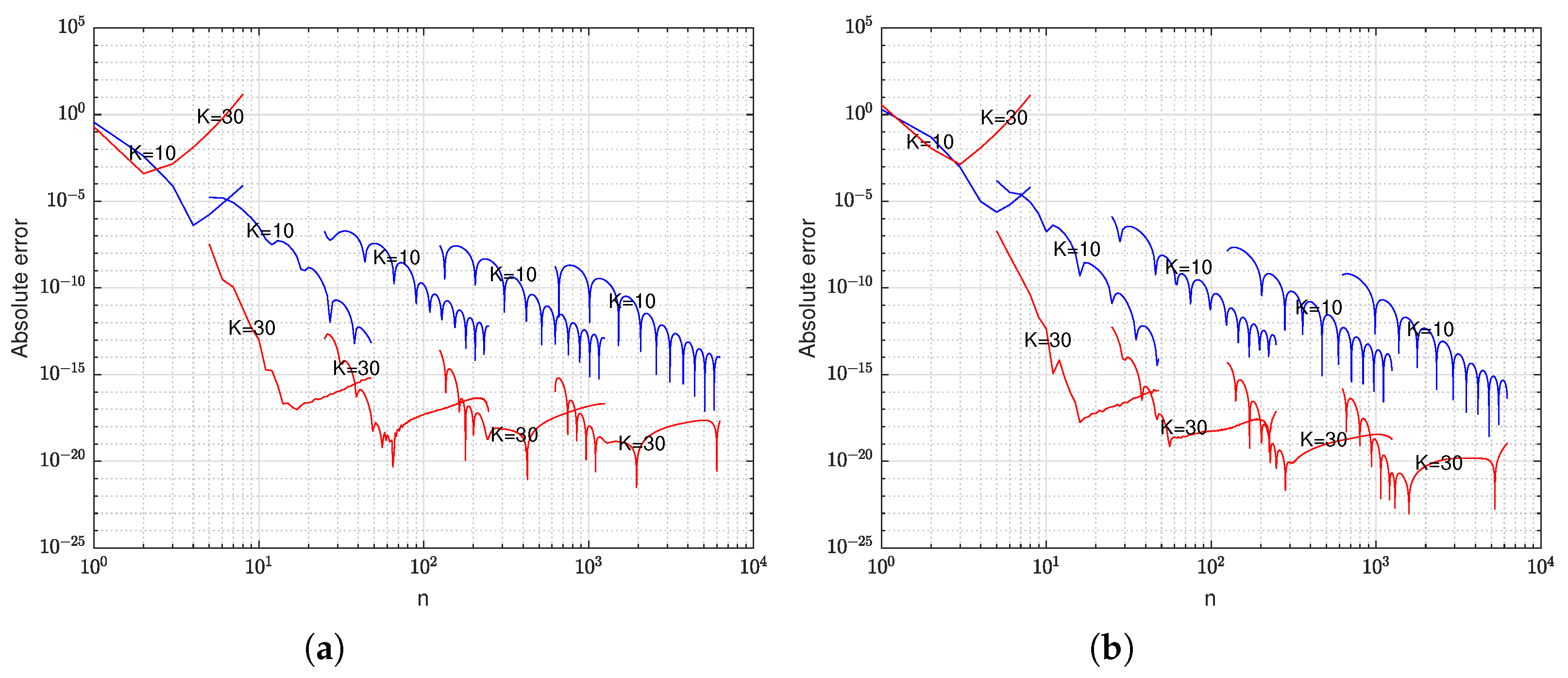
To demonstrate the effectiveness of the approximation, we subtract (57) from (9) and obtain the absolute value, which represents the absolute approximation error. Setting $B=5$, $I_l(l=1,2,3,4,5),$ and $K=10$ and 30, we plot the absolute approximation error in Figure 1.

Figure 1. (a) Absolute error for ${\omega }_n^{\left(0.3\right)}$ with $\tau ={10}^{-3}$, (b) absolute error for ${\omega }_n^{(-0.3)}$ with $\tau ={10}^{-3}$.

Figure 1 shows that the approximate effect of the first few weights is poor, so in the calculation process, we calculate the first few weights by (9) and find that the approximate effect of $K=30$ is generally better than that of $K=10$, which will be verified in Example 4. Referring to [32], we determine L and obtain $n=b_0>b_1>\cdots >b_{L-1}>b_L=0$.

Now, we rewrite (8) as

$$\begin{array}{cc}\hfill & D_{\tau ,\eta }^{n,\theta }\xi ={\tau }^{-\eta }{\omega }_0^{\left(\eta \right)}({\xi }^n-{\xi }^0)+{\tau }^{-\eta }\sum _{l=1}^L\sum _{k=b_l}^{b_{l-1}-1}{\omega }_{n-k}^{\left(\eta \right)}({\xi }^k-{\xi }^0),\hfill \\ \hfill & I_{\tau ,\eta }^{n,\theta }\xi ={\tau }^{\eta }{\omega }_0^{(-\eta )}({\xi }^n-{\xi }^0)+{\tau }^{\eta }\sum _{l=1}^L\sum _{k=b_l}^{b_{l-1}-1}{\omega }_{n-k}^{(-\eta )}({\xi }^k-{\xi }^0).\hfill \end{array}$$

(59)

We define $u_{n,\delta }^{\left(l\right)}$ as

$$u_{n,\delta }^{\left(l\right)}=\left\{\begin{array}{ccc}{\tau }^{-\delta }{\omega }_0^{\left(\delta \right)}({\xi }^n-{\xi }^0),\hfill & \hfill & l=0\hfill \\ {\tau }^{-\delta }\sum _{k=b_l}^{b_{l-1}-1}{\omega }_{n-k}^{\left(\delta \right)}({\xi }^k-{\xi }^0).\hfill & \hfill & l=1,2,\cdots ,L\hfill \end{array}\right.$$

(60)

Then, utilizing (57), (60), and the definitions for $e_n^{\left(i\right)}\left(z\right)(i=1,2)$, we obtain (for $l>0$)

$$\begin{array}{cc}\hfill u_{n,\delta }^{\left(l\right)}\approx & \sum _{j=-K}^K{w}_j^{\left(l\right)}\left[\tau \sum _{k=b_l}^{b_{l-1}-1}{e}_{n-k}^{\left(\kappa \right)}\left(\tau {\lambda }_j^{\left(l\right)}\right)({\xi }^k-{\xi }^0)\right]F_{\delta }\left({\lambda }_j^{\left(l\right)}\right)\hfill \\ \hfill =& \sum _{j=-K}^K{w}_j^{\left(l\right)}\tau \left[\sum _{k=b_l}^{b_{l-1}-1}{e}_{n-k}^{\left(1\right)}\left(\tau {\lambda }_j^{\left(l\right)}\right)({\xi }^k-{\xi }^0)-\sum _{k=b_l}^{b_{l-1}-1}{e}_{n-k}^{\left(2\right)}\left(\tau {\lambda }_j^{\left(l\right)}\right)({\xi }^k-{\xi }^0)\right]F_{\delta }\left({\lambda }_j^{\left(l\right)}\right)\hfill \\ \hfill =& \sum _{j=-K}^K{w}_j^{\left(l\right)}\left[r_1^{n-(b_{l-1}-1)}\left(\tau {\lambda }_j^{\left(l\right)}\right)v_j^{\left(1\right)}-r_2^{n-(b_{l-1}-1)}\left(\tau {\lambda }_j^{\left(l\right)}\right)v_j^{\left(2\right)}\right]F_{\delta }\left({\lambda }_j^{\left(l\right)}\right)\hfill \end{array}$$

(61)

where $v_j^{\left(i\right)}(i=1,2)$ is as follows

$$v_j^{\left(i\right)}=v_j^{\left(i\right)}(b_l,b_{l-1},{\lambda }_j^{\left(l\right)})=\tau \sum _{k=b_l}^{b_{l-1}-1}{e}_{(b_{l-1}-1)-k}^{\left(i\right)}\left(\tau {\lambda }_j^{\left(l\right)}\right)({\xi }^k-{\xi }^0).$$

(62)

We notice that $v_j^{\left(i\right)}(b_l,b_{l-1},{\lambda }_j^{\left(l\right)})$ has a recursive structure, which can be utilized to enhance the computation speed:

$$\begin{array}{cc}\hfill v_j^{\left(i\right)}(b_l,b_s,{\lambda }_j^{\left(l\right)})=& \tau \sum _{k=b_l}^{b_m-1}{e}_{(b_s-1)-k}^{\left(i\right)}\left(\tau {\lambda }_j^{\left(l\right)}\right)(u^k-u^0)+v_j^{\left(i\right)}(b_m,b_s,{\lambda }_j^{\left(l\right)})\hfill \\ \hfill =& r_i{\left(\tau {\lambda }_j^{\left(l\right)}\right)}^{b_s-b_m}{v}_j^{\left(i\right)}(b_l,b_m,{\lambda }_j^{\left(l\right)})+v_j^{\left(i\right)}(b_m,b_s,{\lambda }_j^{\left(l\right)}).\hfill \end{array}$$

(63)

The first few weights are not described well by (57) (refer to Figure 1). Thus, for $l=0,1,2,\cdots ,k$, we calculate the weights according to (9), and for $l=k+1,\cdots ,L$, we calculate the weights according to (57). Combining (59)–(61), we can obtain

$$\begin{array}{cc}& D_{\tau ,\eta }^{n,\theta }\xi =\sum _{l=0}^k{u}_{n,\eta }^{\left(l\right)}+\sum _{l=k+1}^L{u}_{n,\eta }^{\left(l\right)}\hfill \\ \hfill \approx & \sum _{l=0}^k{u}_{n,\eta }^{\left(l\right)}+\sum _{l=k+1}^L\sum _{j=-K}^K{w}_j^{\left(l\right)}\left[r_1^{n-(b_{l-1}-1)}\left(\tau {\lambda }_j^{\left(l\right)}\right)v_j^{\left(1\right)}-r_2^{n-(b_{l-1}-1)}\left(\tau {\lambda }_j^{\left(l\right)}\right)v_j^{\left(2\right)}\right]F_{\eta }\left({\lambda }_j^{\left(l\right)}\right).\hfill \\ & I_{\tau ,\eta }^{n,\theta }\xi =\sum _{l=0}^k{u}_{n,-\eta }^{\left(l\right)}+\sum _{l=k+1}^L{u}_{n,-\eta }^{\left(l\right)}\hfill \\ \hfill \approx & \sum _{l=0}^k{u}_{n,-\eta }^{\left(l\right)}+\sum _{l=k+1}^L\sum _{j=-K}^K{w}_j^{\left(l\right)}\left[r_1^{n-(b_{l-1}-1)}\left(\tau {\lambda }_j^{\left(l\right)}\right)v_j^{\left(1\right)}-r_2^{n-(b_{l-1}-1)}\left(\tau {\lambda }_j^{\left(l\right)}\right)v_j^{\left(2\right)}\right]F_{-\eta }\left({\lambda }_j^{\left(l\right)}\right).\hfill \end{array}$$

(64)

Below are listed the steps for implementing the fast algorithm:

1.

Input parameters $B$, $K$, ${\lambda }_j^{\left(l\right)}$, $w_j^{\left(l\right)}$, ${\vartheta }_j$.

2.

Compute $b_l$ and obtain $n=b_0>b_1>\cdots >b_{L-1}>b_L=0$.

3.

For $l=0,1,2,\cdots ,k$, compute the weights using (9), and calculate the weights using (57) for $l=k+1,\cdots ,L$.

4.

From step 3, compute (64).

6. Numerical Examples

In this section, we provide four examples of solving an FKGE utilizing our proposed scheme, and the results verify our theoretical analysis and the effectiveness of our method. The basis function was chosen as $\psi \left(x\right)=L_j\left(x\right)-L_{j+2}\left(x\right),j=0,1,\cdots ,N$ for $\forall v_N^k\in P_N^0,v_N^k={\sum }_{j=0}^{N-2}{\widehat{v}}_N^k{\psi }_j\left(x\right)$, where ${\widehat{v}}_N^k$ is the frequency coefficient. The codes were developed in MATLAB 2022a and executed on a Windows 10 operating system. The computer used for running these codes had a processor speed of 2.60 GHz and 8 GB of RAM.

Example 1.

Let $\rho =1$ in (1). We considered the following fractional dissipative Klein–Gordon equation with homogeneous initial condition $\varphi \left(x\right)=0,\phi \left(x\right)=0$:

$$\frac{{\partial }^{\alpha }\xi (x,t)}{\partial t^{\alpha }}+\frac{\partial \xi (x,t)}{\partial t}+\xi (x,t)=\frac{{\partial }^2\xi (x,t)}{\partial x^2}+f(x,t).$$

(65)

Assuming that the exact solution of Equation (65) is $\xi (x,t)=t^{4}sin\left(\pi x\right)$, the corresponding forcing term is given by

$$f(x,t)=\left[\frac{\mathsf{\Gamma }\left(5\right)}{\mathsf{\Gamma }(5-\alpha )}{t}^{4-\alpha }+4t^3+(1+{\pi }^2)t^4\right]sin\left(\pi x\right).$$

For $N=100$, the results are presented in Table 1, Table 2 and Table 3. It can be observed that our numerical scheme exhibited second-order convergence accuracy in the temporal direction, which aligned with the theoretical expectations.

Table 1. The $L^2$ error and $L^{\infty }$ error at $\alpha =1.5$, $\theta =0.3$, and $T=1$.

$\mathit{\tau }$	${\mathit{L}}^2$ Error	Rate	${\mathit{L}}^{\mathit{\infty }}$ Error	Rate	Time (s)
$2^{-6}$	5.044987 × 10${}^{-3}$		8.532442 × 10${}^{-4}$		0.306217
$2^{-7}$	1.280432 × 10${}^{-3}$	1.98	2.165557 × 10${}^{-4}$	1.98	0.766249
$2^{-8}$	3.225111 × 10${}^{-4}$	1.99	5.454538 × 10${}^{-5}$	1.99	3.059746
$2^{-9}$	8.092851 × 10${}^{-5}$	1.99	1.368721 × 10${}^{-5}$	1.99	15.242314
$2^{-10}$	2.026974 × 10${}^{-5}$	2.00	3.428163 × 10${}^{-6}$	2.00	78.373508

Table 2. Temporal convergence rates at $\alpha =1.2$, $\theta =0.5$, and $T=1$.

$\mathit{\tau }$	${\mathit{L}}^2$ Error	Rate	${\mathit{L}}^{\mathit{\infty }}$ Error	Rate	Time (s)
$2^{-6}$	6.613273 × 10${}^{-3}$		1.118484 × 10${}^{-3}$		0.279892
$2^{-7}$	1.674942 × 10${}^{-3}$	1.98	2.832782 × 10${}^{-4}$	1.98	0.749574
$2^{-8}$	4.214538 × 10${}^{-4}$	1.99	7.127927 × 10${}^{-5}$	1.99	3.058692
$2^{-9}$	1.057042 × 10${}^{-4}$	2.00	1.787745 × 10${}^{-5}$	2.00	14.168706
$2^{-10}$	2.646869 × 10${}^{-5}$	2.00	4.476574 × 10${}^{-6}$	2.00	78.849718

Table 3. The $L^2$ error and $L^{\infty }$ error at $\alpha =1.8$, $\theta =0.8$, and $T=1$.

$\mathit{\tau }$	${\mathit{L}}^2$ Error	Rate	${\mathit{L}}^{\mathit{\infty }}$ Error	Rate	Time (s)
$2^{-6}$	1.584784 × 10${}^{-2}$		2.680300 × 10${}^{-3}$		0.267496
$2^{-7}$	4.066127 × 10${}^{-3}$	1.96	6.876924 × 10${}^{-4}$	1.96	0.729302
$2^{-8}$	1.029638 × 10${}^{-3}$	1.98	1.741398 × 10${}^{-4}$	1.98	3.289171
$2^{-9}$	2.590520 × 10${}^{-4}$	1.99	4.381272 × 10${}^{-5}$	1.99	14.103777
$2^{-10}$	6.496853 × 10${}^{-5}$	2.00	1.098794 × 10${}^{-5}$	2.00	77.813919

To analyze the spatial accuracy, we set $\tau =0.001$ to eliminate temporal direction errors. In Figure 2, it can be observed that when $\alpha =1.8$ and $\theta =0.3,$ the error exhibited an exponential decrease. This behavior confirmed the spectral accuracy of the method, which in turn confirmed the validity of our theoretical analysis.

Figure 2. $\alpha =1.8, \theta =0.8$ for Example 1 at $T=1$.

Example 2.

Let $\rho =0$ in (1). We investigated the fractional linear Klein–Gordon equation with the non-homogeneous initial conditions $\varphi \left(x\right)=sin\left(\pi x\right),$$\phi \left(x\right)=0,$

$$\frac{{\partial }^{\alpha }\xi (x,t)}{\partial t^{\alpha }}+\xi (x,t)=\frac{{\partial }^2\xi (x,t)}{\partial x^2}+f(x,t).$$

(66)

Assuming that the exact solution of Equation (66) is $\xi (x,t)=(t^4+1)sin\left(\pi x\right)$, the corresponding forcing term is

$$f(x,t)=\left[\frac{\mathsf{\Gamma }\left(5\right)}{\mathsf{\Gamma }(5-\alpha )}{t}^{4-\alpha }+\frac{1}{\mathsf{\Gamma }(1-\alpha )}{t}^{-\alpha }+(t^4+1)(1+{\pi }^2)\right]sin\left(\pi x\right).$$

For $N=100$, the results are illustrated in Table 4, Table 5 and Table 6. Notably, even when considering non-homogeneous initial conditions, it was evident that our numerical scheme remained applicable. The results indicated the adaptability and flexibility of our method.

Table 4. The $L^2$ error and $L^{\infty }$ error at $\alpha =1.5$, $\theta =0.9$, and $T=1$.

$\mathit{\tau }$	${\mathit{L}}^2$ Error	Rate	${\mathit{L}}^{\mathit{\infty }}$ Error	Rate	Time (s)
$2^{-6}$	1.637673 × 10${}^{-2}$		2.769750 × 10${}^{-3}$		0.271781
$2^{-7}$	4.181892 × 10${}^{-3}$	1.97	7.072714 × 10${}^{-4}$	1.97	0.695502
$2^{-8}$	1.056485 × 10${}^{-3}$	1.98	1.786803 × 10${}^{-4}$	1.98	2.756914
$2^{-9}$	2.655010 × 10${}^{-4}$	1.99	4.490342 × 10${}^{-5}$	1.99	12.633774
$2^{-10}$	6.654790 × 10${}^{-5}$	2.00	1.125506 × 10${}^{-5}$	2.00	59.670061

Table 5. The $L^2$ error and $L^{\infty }$ error at $\alpha =1.2$, $\theta =0.7$, and $T=1$.

$\mathit{\tau }$	${\mathit{L}}^2$ Error	Rate	${\mathit{L}}^{\mathit{\infty }}$ Error	Rate	Time (s)
$2^{-6}$	1.012134 × 10${}^{-2}$		1.711793 × 10${}^{-3}$		0.275343
$2^{-7}$	2.568689 × 10${}^{-3}$	1.98	4.344350 × 10${}^{-4}$	1.98	0.765448
$2^{-8}$	6.469977 × 10${}^{-4}$	1.99	1.094249 × 10${}^{-4}$	1.99	2.744447
$2^{-9}$	1.623546 × 10${}^{-4}$	1.99	2.745857 × 10${}^{-5}$	1.99	13.364513
$2^{-10}$	4.066441 × 10${}^{-5}$	2.00	6.877456 × 10${}^{-6}$	2.00	60.118435

Table 6. The $L^2$ error and $L^{\infty }$ error at $\alpha =1.8$, $\theta =0.3$, and $T=1$.

$\mathit{\tau }$	${\mathit{L}}^2$ Error	Rate	${\mathit{L}}^{\mathit{\infty }}$ Error	Rate	Time (s)
$2^{-6}$	6.314916 × 10${}^{-3}$		1.068024 × 10${}^{-3}$		0.273913
$2^{-7}$	1.612247 × 10${}^{-3}$	1.97	2.726746 × 10${}^{-4}$	1.97	0.709604
$2^{-8}$	4.072641 × 10${}^{-4}$	1.99	6.887941 × 10${}^{-5}$	1.99	2.833458
$2^{-9}$	1.023419 × 10${}^{-4}$	1.99	1.730879 × 10${}^{-5}$	1.99	12.073551
$2^{-10}$	2.565123 × 10${}^{-5}$	2.00	4.338319 × 10${}^{-6}$	2.00	58.882522

Example 3.

Let $\rho =1$ in (1). The non-smooth solution $\xi (x,t)=(t^4+t^{min\{2-\alpha ,\alpha -1\}})sin\left(\pi x\right)$ was considered, with the corresponding forcing term

$$\begin{array}{cc}\hfill f(x,t)=& [\frac{\mathsf{\Gamma }(min\{3-\alpha ,\alpha \left\}\right)}{\mathsf{\Gamma }(min\{3-2\alpha ,0\left\}\right)}{t}^{min\{2-2\alpha ,-1\}}+\frac{\mathsf{\Gamma }\left(5\right)}{\mathsf{\Gamma }(5-\alpha )}{t}^{4-\alpha }+4t^3+\hfill \\ & min\{2-\alpha ,\alpha -1\}{t}^{min\{1-\alpha ,\alpha -2\}}+(t^4+t^{min\{2-\alpha ,\alpha -1\}})(1+{\pi }^2)]sin\left(\pi x\right).\hfill \end{array}$$

Assuming $N=100$, it is worth mentioning that due to the weak regularity of the solution, it was not possible to achieve the optimal convergence rate of $O\left({\tau }^2\right)$. Referring to Table 7, we can observe that the inclusion of correction terms led to an improved convergence rate. This result serves as evidence for the efficiency of our method.

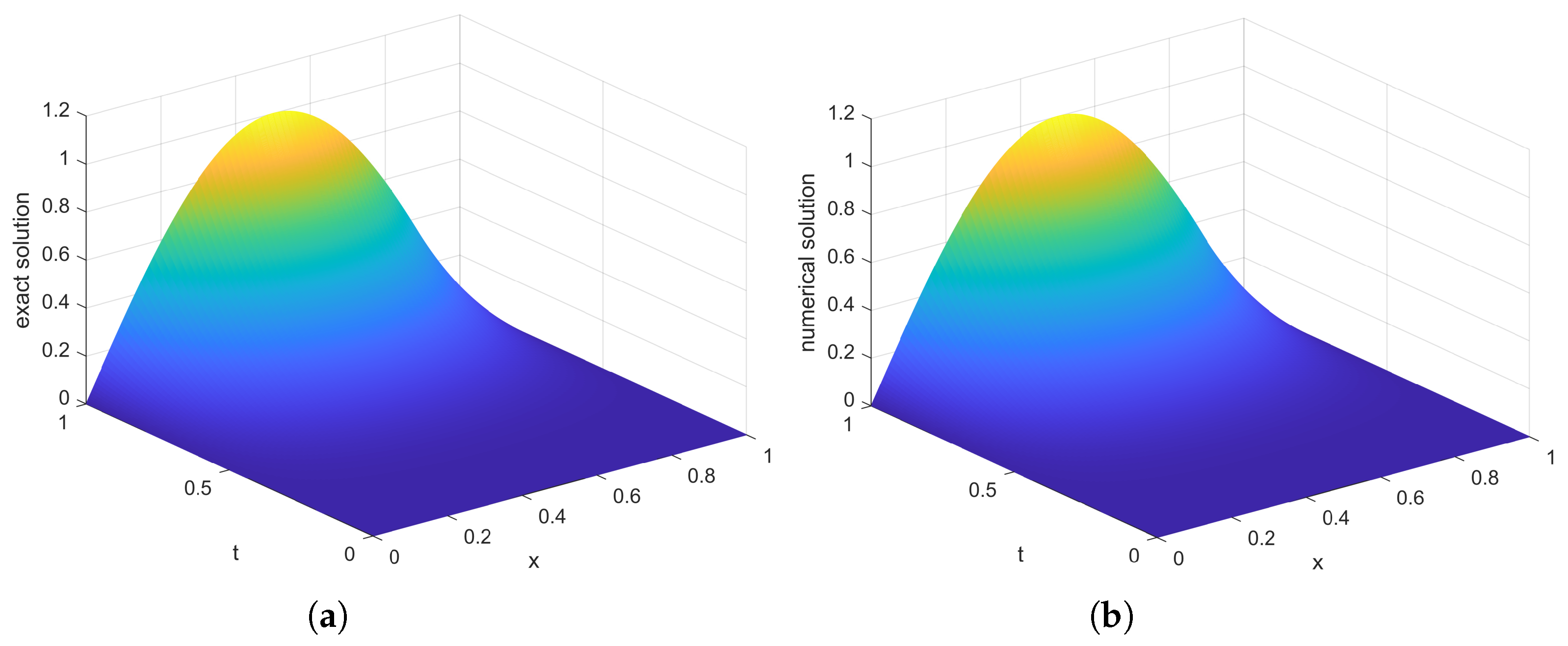
Table 7. Temporal convergence rates at $T=1$.

($\mathit{\alpha },\mathit{\theta }$)	$\mathit{\tau }$	Direct Method	Rate	Correction	Rate
(1.2, 0.1)	$2^{-4}$	1.154038 × 10${}^{-3}$		4.645596 × 10${}^{-4}$
	$2^{-5}$	3.103449 × 10${}^{-4}$	1.89	1.184401 × 10${}^{-4}$	1.97
	$2^{-6}$	8.260221 × 10${}^{-5}$	1.91	2.815017 × 10${}^{-5}$	2.07
	$2^{-7}$	2.255211 × 10${}^{-5}$	1.87	7.023850 × 10${}^{-6}$	2.00
(1.8, 0.3)	$2^{-4}$	1.538917 × 10${}^{-2}$		1.124338 × 10${}^{-2}$
	$2^{-5}$	4.237714 × 10${}^{-3}$	1.86	2.942242 × 10${}^{-3}$	1.93
	$2^{-6}$	1.171468 × 10${}^{-3}$	1.85	7.246667 × 10${}^{-4}$	2.02
	$2^{-7}$	3.333848 × 10${}^{-4}$	1.81	1.757115 × 10${}^{-4}$	2.04
(1.5, 0)	$2^{-4}$	1.457736 × 10${}^{-3}$		5.482971 × 10${}^{-4}$
	$2^{-5}$	4.355394 × 10${}^{-4}$	1.74	1.518084 × 10${}^{-4}$	1.85
	$2^{-6}$	1.323356 × 10${}^{-4}$	1.72	3.868906 × 10${}^{-5}$	1.97
	$2^{-7}$	4.106669 × 10${}^{-5}$	1.69	9.639184e × 10${}^{-6}$	2.00

Example 4.

Let $\rho =0$ in (1). We utilized the fast algorithm to solve the Equation (66). Assuming that the exact solution of Equation (66) is $\xi (x,t)=t^{4}sin\left(\pi x\right)$, the corresponding forcing term is

$$f(x,t)=\left[\frac{\mathsf{\Gamma }\left(5\right)}{\mathsf{\Gamma }(5-\alpha )}{t}^{4-\alpha }+(1+{\pi }^2)t^4\right]sin\left(\pi x\right).$$

We set $B=5$ and $N=100.$ To simplify the notation, we denoted the approximation of Equation (57) with $2K+1$ points as Fast${}_K$. We had two sets of solutions: $Z_S$, which were obtained using the direct method, and $Z_F$, which was obtained using the fast algorithm. We set $\theta =\frac{1-\alpha }{2}$ and defined the pointwise error as

$$e(\alpha ,M)=\underset{t=t_0,\cdots ,t_M,x=x_1,\cdots ,x_N}{max}|Z_S-Z_F|.$$

(67)

According to Table 8, it is evident that the fast algorithm significantly accelerated the computation process. Moreover, our approach not only attained exceptional precision, but also effectively reduced the computational cost. For example, for $K=30,$ the pointwise error was around ${10}^{-15}$, which was close to the machine accuracy. Figure 3a displays the exact solutions for $M=1000,\alpha =1.8.$ Figure 3b shows the numerical solutions for the given parameters: $M=1000$, $\alpha$ = 1.8, and $K=30$. Furthermore, in order to obtain the error contour plot shown in Figure 4a, we subtracted the corresponding solutions from Figure 3a,b. In Figure 4b, it is evident that the computational complexity of the fast algorithm was $O(MlogM)$, while the direct method had a computational complexity of $O\left(M^2\right)$. This result in Figure 4 aligned with the theoretical expectations and confirmed that the algorithms’ performances matched the expected efficiencies.

Table 8. Pointwise error with $\theta =\frac{1-\alpha }{2}$.

$\mathit{\alpha }$	M	Direct Method	Fast${}_{10}$	$\mathit{e}\mathbf{(}\mathit{\alpha }\mathbf{,}\mathit{M}\mathbf{)}$	Fast${}_{30}$	$\mathit{e}\mathbf{(}\mathit{\alpha }\mathbf{,}\mathit{M}\mathbf{)}$
$1.8$	$1\times {10}^3$	56.29 s	6.96 s	2.11210 × 10${}^{-8}$	16.08 s	3.16414 × 10${}^{-15}$
	$2\times {10}^3$	307.52 s	18.44 s	2.22114 × 10${}^{-8}$	42.53 s	7.16094 × 10${}^{-14}$
	$3\times {10}^3$	909.11 s	36.25 s	5.83438 × 10${}^{-8}$	84.64 s	1.33227 × 10${}^{-15}$
$1.5$	$1\times {10}^3$	57.41 s	6.51 s	3.94038 × 10${}^{-7}$	16.55 s	5.62052 × 10${}^{-16}$
	$2\times {10}^3$	310.38 s	18.48 s	4.21263 × 10${}^{-7}$	44.76 s	2.57572 × 10${}^{-14}$
	$3\times {10}^3$	998.17 s	37.36 s	3.67259 × 10${}^{-7}$	87.23 s	1.52101 × 10${}^{-14}$
$1.2$	$1\times {10}^3$	57.25 s	6.94 s	2.54602 × 10${}^{-7}$	16.55 s	1.85407 × 10${}^{-14}$
	$2\times {10}^3$	308.97 s	18.45 s	5.35331 × 10${}^{-7}$	44.76 s	7.86038 × 10${}^{-14}$
	$3\times {10}^3$	1014.26 s	35.09 s	7.14741 × 10${}^{-8}$	83.61 s	5.17364 × 10${}^{-14}$

Figure 3. (a) Exact solution, (b) numerical solution.

Figure 4. (a) Error contour, (b) computational complexity.

7. Conclusions

In this study, we developed a stable and efficient numerical method to solve an FKGE. A stability analysis and the convergence of the discrete scheme were provided in our method. Considering the weak regularity of the solutions, we improved the convergence order by incorporating correction terms into our approach. To optimize the computational complexity, we implemented a fast algorithm, which significantly reduced the runtime required for solving an FKGE. This allowed for quicker computations without sacrificing accuracy. We note the method can be extended to higher-dimensional cases.

References

- Akgul, A.; Partohaghighi, M. New fractional modelling and control analysis of the circumscribed self-excited spherical strange attractor. Chaos Solitons Fractals 2022, 158, 111956. [Google Scholar] [CrossRef]
- Nabi, K.N.; Kumar, P.; Erturk, V.S. Projections and fractional dynamics of covid-19 with optimal control strategies. Chaos Solitons Fractals 2021, 145, 110689. [Google Scholar] [CrossRef] [PubMed]
- de Sousa, F.B.; Babu, P.K.V.; Radmacher, M.; Oliveira, C.L.N.; de Sousa, J.S. Multiple power-law viscoelastic relaxation in time and frequency domains with atomic force microscopy. J. Phys. D Appl. Phys. 2021, 54, 335401. [Google Scholar] [CrossRef]
- Chen, Y.W.; Wen, G.G.; Rahmani, A.; Huang, T.W. Heterogeneous multiagent systems with different fractional order: An experience-based fusion controller. IEEE Trans. Circuits Syst. II Express Briefs 2022, 69, 3520–3524. [Google Scholar] [CrossRef]
- Dubey, V.P.; Kumar, D.; Singh, J.; Alshehri, A.M.; Dubey, S. Analysis of local fractional klein-gordon equations arising in relativistic fractal quantum mechanics. Waves Random Complex Media 2022, 32, 1–21. [Google Scholar] [CrossRef]
- Cheng, W.; Chen, R.P.; Yin, Z.Y.; Wang, H.L.; Meng, F.Y. A fractional-order two-surface plasticity model for over-consolidated clays and its application to deep gallery excavation. Comput. Geotech. 2023, 159, 105494. [Google Scholar] [CrossRef]
- Malik, S.A.; Mir, A.H. Fpga realization of fractional order neuron. Appl. Math. Model. 2020, 81, 372–385. [Google Scholar] [CrossRef]
- Gao, Y.F.; Yin, D.S.; Tang, M.; Zhao, B. A three-dimensional fractional visco-hyperelastic model for soft materials. J. Mech. Behav. Biomed. 2023, 137, 105564. [Google Scholar] [CrossRef]
- Feng, L.B.; Liu, F.W.; Turner, I.; Zheng, L.C. Novel numerical analysis of multi-term time fractional viscoelastic non-newtonian fluid models for simulating unsteady mhd couette flow of a generalized Oldroyd-B fluid. Fract. Calc. Appl. Anal. 2018, 21, 1073–1103. [Google Scholar] [CrossRef]
- Rekha, J.; Suma, S.P.; Shilpa, B.; Khan, U.; Hussain, S.M.; Zaibk, A.; Galal, A.M. Solute transport exponentially varies with time in an unsaturated zone using finite element and finite difference method. Int. J. Mod. Phys. B 2023, 37, 2350089. [Google Scholar] [CrossRef]
- Yin, B.L.; Liu, Y.; Li, H.; Zeng, F.H. A class of efficient time-stepping methods for multi-term time-fractional reaction-diffusion-wave equations. Appl. Numer. Math. 2021, 165, 56–82. [Google Scholar] [CrossRef]
- Liu, Y.; Du, Y.W.; Li, H.; Liu, F.W.; Wang, Y.J. Some second-order schemes combined with finite element method for nonlinear fractional cable equation. Numer. Algorithms 2019, 80, 533–555. [Google Scholar] [CrossRef]
- Yin, B.L.; Liu, Y.; Li, H.; Zhang, Z.M. Efficient shifted fractional trapezoidal rule for subdiffusion problems with nonsmooth solutions on uniform meshes. BIT Numer. Math. 2022, 62, 631–666. [Google Scholar] [CrossRef]
- Saffarian, M.; Mohebbi, A. Finite difference spectral element method for one and two dimensional Riesz space fractional advection dispersion equations. Math. Comput. Simulat. 2022, 193, 348–370. [Google Scholar] [CrossRef]
- Zheng, R.M.; Jiang, X.Y. Spectral methods for the time-fractional Navier-Stokes equation. Appl. Math. Lett. 2019, 91, 194–200. [Google Scholar] [CrossRef]
- Liu, Z.T.; Lu, S.J.; Liu, F.W. Fully discrete spectral methods for solving time fractional nonlinear sine-gordon equation with smooth and non-smooth solutions. Appl. Math. Comput. 2018, 333, 213–224. [Google Scholar] [CrossRef]
- Zeng, F.H.; Zhang, Z.Q.; Karniadakis, G.E. Second-order numerical methods for multi-term fractional differential equations: Smooth and non-smooth solutions. Comput. Methods Appl. Mech. Eng. 2017, 327, 478–502. [Google Scholar] [CrossRef]
- Dehghan, M.; Abbaszadeh, M. Spectral element technique for nonlinear fractional evolution equation, stability and convergence analysis. Appl. Numer. Math. 2017, 119, 51–66. [Google Scholar] [CrossRef]
- Hashemizadeh, E.; Ebrahimzadeh, A. An efficient numerical scheme to solve fractional diffusion-wave and fractional klein-gordon equations in fluid mechanics. Physica A 2018, 503, 1189–1203. [Google Scholar] [CrossRef]
- Zhang, X.; Yang, B.; Wei, C.Z.; Luo, M.K. Quantization method and Schrodinger equation of fractional time and their weak effects on Hamiltonian: Phase transitions of energy and wave functions. Commun. Nonlinear Sci. 2021, 93, 105531. [Google Scholar] [CrossRef]
- Dartora, C.A.; Zanella, F.; Cabrera, G.G. Emergence of fractional quantum mechanics in condensed matter physics. Phys. Lett. A 2021, 415, 127643. [Google Scholar] [CrossRef]
- Ghosh, U.; Banerjee, J.; Sarkar, S.; Das, S. Fractional Klein-Gordon equation composed of Jumarie fractional derivative and its interpretation by a smoothness parameter. Pramana 2018, 90, 74. [Google Scholar] [CrossRef]
- Vong, S.; Wang, Z.B. A high-order compact scheme for the nonlinear fractional klein-gordon equation. Numer. Methods Partial Differ. Equ. 2015, 31, 706–722. [Google Scholar] [CrossRef]
- Khader, M.M.; Kumar, S. An accurate numerical method for solving the linear fractional klein-gordon equation. Math. Methods Appl. Sci. 2014, 37, 2972–2979. [Google Scholar] [CrossRef]
- Saffarian, M.; Mohebbi, A. Numerical solution of two and three dimensional time fractional damped nonlinear klein-gordon equation using adi spectral element method. Appl. Math. Comput. 2021, 405, 126182. [Google Scholar] [CrossRef]
- Jin, B.; Li, B.; Zhou, Z. An analysis of the Crank-Nicolson method for subdiffusion. IMA J. Numer. Anal. 2018, 38, 518–541. [Google Scholar] [CrossRef]
- Zhang, H.; Jiang, X.Y.; Zeng, F.H. An H-1 convergence of the spectral method for the time-fractional non-linear diffusion equations. Adv. Comput. Math. 2021, 47, 63. [Google Scholar] [CrossRef]
- Zhang, H.; Zeng, F.H.; Jiang, X.Y.; Karniadakis, G.E. Convergence analysis of the time-stepping numerical methods for time-fractional nonlinear subdiffusion equations. Fract. Calc. Appl. Anal. 2022, 25, 453–487. [Google Scholar] [CrossRef]
- Zeng, F.H.; Turner, I.; Burrage, K. A stable fast time-stepping method for fractional integral and derivative operators. J. Sci. Comput. 2018, 77, 283–307. [Google Scholar] [CrossRef]
- Huang, Y.X.; Li, Q.G.; Li, R.X.; Zeng, F.H.; Guo, L. A unified fast memory-saving time-stepping method for fractional operators and its applications. Numer. Math. Theory Methods Appl. 2022, 5, 679–714. [Google Scholar] [CrossRef]
- Weideman, J. Optimizing Talbot’s contours for the inversion of the Laplace transform. SIAM J. Numer. Anal. 2006, 44, 2342–2362. [Google Scholar] [CrossRef]
- Schädle, A.; López-Fernández, M.; Lubich, C. Fast and oblivious convolution quadrature. SIAM J. Sci. Comput. 2006, 28, 421–438. [Google Scholar] [CrossRef]
Disclaimer/Publisher’s Note: The statements, opinions and data contained in all publications are solely those of the individual author(s) and contributor(s) and not of MDPI and/or the editor(s). MDPI and/or the editor(s) disclaim responsibility for any injury to people or property resulting from any ideas, methods, instructions or products referred to in the content. |
© 2023 by the authors. Licensee MDPI, Basel, Switzerland. This article is an open access article distributed under the terms and conditions of the Creative Commons Attribution (CC BY) license (https://creativecommons.org/licenses/by/4.0/).