Numerical Analysis of Direct and Inverse Problems for a Fractional Parabolic Integro-Differential Equation

Abstract

A mathematical model consisting of weakly coupled time fractional one parabolic PDE and one ODE equations describing dynamical processes in porous media is our physical motivation. As is often performed, by solving analytically the ODE equation, such a system is reduced to an integro-parabolic equation. We focus on the numerical reconstruction of a diffusion coefficient at finite number space-points measurements. The well-posedness of the direct problem is investigated and energy estimates of their solutions are derived. The second order in time and space finite difference approximation of the direct problem is analyzed. The approach of Lagrangian multiplier adjoint equations is utilized to compute the Fréchet derivative of the least-square cost functional. A numerical solution based on the conjugate gradient method (CGM) of the inverse problem is studied. A number of computational examples are discussed.

1. Introduction

The second-order hyperbolic and parabolic systems of partial differential equations, as well as coupled PDE-ODE systems, are a substantial theoretical foundation for many mathematical and engineering problems [1,2,3,4,5,6,7,8,9,10]. In the present paper, we concentrate on the features of a parabolic PDE-ODE system.

Recently, because of the the many applications, fractional integro-differential equations are the focus of a large body of results. The classical integer order derivative is a local operator, which is not adequate for a description of many processes in physics, mechanics, industrial finance, etc. The fractional derivative is a nonlocal operator, which is often used to model phenomena in heat mass transfer [4,5,11], medicine [12], viscoelastic materials [8,13], porous media [1,5,7,10,14,15], mathematical biology and in particularly the honeybee population [16], mathematical finance and economics—see [17,18] and references therein—and atmosphere pollution [6,19].

In [4], analytical exact solutions to the neutron fractional parabolic PDE-ODE system are derived. The inverse problems (IPs) of differential equations with time fractional derivatives concern the recovery of a variety unknown parameters, such as source term, fractional order, coefficients, etc. For instance, Georgiev and Vulkov [16] present a numerical study of the inverse problem for coefficient determination in honeybee population models with Caputo and Caputo–Fabrizio time fractional derivative, and in [13] a parameter identification inverse problem is studied.

In this work, we numerically recover the unknown diffusion coefficient for a time fractional integro-diffusion convection reaction equation, obtained from a model system of differential equations.

A System of a Parabolic and a Ordinary Differential Equation

As a simple physical motivation, we consider a model of non-Darcian flow in transport media used to describe different real processes, see, e.g., [3,5,7,8,10,20].

Suppose that diffusion and solute transport initiate within the mobile phase, while the change in solute concentration within the immobile phase is a dynamic process influenced by the porous media’s low permeability and significant heterogeneity. The fractional calculus has been introduced as an efficient tool for modeling. A general form of a differential equation system that describes such processes reads as follows [3,5,7,20]:

$$\begin{array}{c}\frac{{\partial }^{\alpha }u}{\partial t^{\alpha }}-\frac{\partial }{\partial x}\left(a\left(x\right)\frac{\partial u}{\partial x}-v\left(x\right)u\right)+r\lambda \left(x\right)(u-w)=0\mathrm{in}{Q}_T=\Omega \times (0,T),\Omega =(0,l),\hfill \end{array}$$

(1)

$$\begin{array}{c}\frac{{\partial }^{{\alpha }_1}w}{\partial t^{{\alpha }_1}}+\lambda \left(x\right)w=\lambda \left(x\right)u\mathrm{in}{Q}_T.\hfill \end{array}$$

(2)

with the initial condition and appropriate boundary conditions. Here, $0<\alpha ,{\alpha }_1\le 1$ and

$$\frac{{\partial }^{\alpha }v}{\partial t^{\alpha }}=\frac{1}{\Gamma (1-\alpha )}{\int }_0^t{(t-s)}^{-\alpha }\frac{\partial v}{\partial s}(x,s)\mathrm{d}s$$

(3)

is the pointwise Caputo derivative [13,21,22,23]. With u and w are denoted the concentration of a contaminant in the relevant phases. The authors of [24] using Equation (2) write an integral formula for $w(x,t)$ and placed it in (1) to obtain an integro-differential equation for $u(x,t)$, $(x,t)\in Q_T$. On this basis, we consider a more general equation:

$$\begin{array}{c}\hfill \begin{array}{cc}\hfill \frac{{\partial }^{\alpha }u}{\partial t^{\alpha }}=& \frac{\partial }{\partial x}\left(a(x,t)\frac{\partial u}{\partial x}\right)+b(x,t)\frac{\partial u}{\partial x}+c(x,t)u+{\int }_0^t\rho (x,t,s)u(x,s)ds+f(x,t)\hfill \\ \hfill =& Zu+f.\hfill \end{array}\end{array}$$

(4)

The remainder of the paper is constructed as follows. In Section 2, we give some notations and discuss the well-posedness of the direct problem. Section 3 is devoted to the numerical solution of the direct problem. In Section 4, we introduce the IP and study its quasisolution. In Section 5, we introduce a finite difference method, combined with the conjugate gradient method (CGM) to solve the IP. Section 6 presents computational results that validate the analysis and demonstrate the efficiency of the proposed algorithm. Some comments and conclusions finalized this paper.

2. Well-Posedness of the Direct Problem

In the IP, it is assumed in advance that the corresponding direct problem is well-posed. The main purpose of this section is the discussion of this question. In this section, our main focus is on the discussion of this question. We consider the Equation (4), $0<a_0\le a(x,t)\le a_1$, $(x,t)\in {\overline{Q}}_T$ and with no loss of generality, zero Dirichlet boundary conditions

$$u(0,t)=0,u(l,t)=0,$$

(5)

and initial condition

$$u(x,0)=u_0\left(x\right).$$

(6)

2.1. Notations and Preliminaries

In the following, we assume classical interpretations of fractional calculus and equations and will refer to monographs [22,23]. Further, let

$$L^p(0,T):=\left\{v:{\int }_0^T{\left|v\left(t\right)\right|}^p\mathrm{d}t<\infty \right\}$$

with $p\ge 1$ and

$$W^{1,1}(0,T):=\left\{v\in L^1(0,T):\frac{\mathrm{d}v}{\mathrm{d}t}\in L^1(0,T)\right\},$$

where the norms are conventionally established by

$${\parallel v\parallel }_{L^p(0,T)}:={\left({\int }_0^T{\left|v\left(t\right)\right|}^{p}dt\right)}^{1/p}{,\parallel v\parallel }_{W^{1,1}(0,T)}:={\parallel v\parallel }_{L^1(0,T)}+{∥\frac{\mathrm{d}v}{\mathrm{d}t}∥}_{L^1(0,T)}.$$

In view of the Young inequality on the convolution, it could be directly established that the classical Caputo derivative (3) could be well-defined for

$$v\in W^{1,1}(0,T)\mathrm{and}\frac{{\mathrm{d}}^{\alpha }v}{\mathrm{d}{t}^{\alpha }}\in L^1(0,T).$$

The Riemann–Liouville left and right integrals of fractional order $\alpha$ are defined as follows [22,23]:

$$\left(I_{0+}^{\alpha }u\right)\left(t\right)=\frac{1}{\Gamma \left(\alpha \right)}{\int }_0^t\frac{u\left(s\right)}{{(t-s)}^{1\alpha }}\mathrm{d}s,\left(I_{T-}^{\alpha }u\right)\left(t\right)=\frac{1}{\Gamma \left(\alpha \right)}{\int }_t^T\frac{u\left(s\right)}{{(s-t)}^{1\alpha }}\mathrm{d}s,$$

and the corresponding Riemann–Liouville left and right fractional derivatives for $0<\alpha <1$ are defined as

$$\begin{array}{cc}\hfill \left(D_{0+}^{\alpha }u\right)\left(t\right)& =\frac{1}{\Gamma (1-\alpha )}\frac{\mathrm{d}}{\mathrm{d}t}{\int }_0^t\frac{u\left(s\right)}{{(t-s)}^{\alpha }}\mathrm{d}s=\frac{\mathrm{d}}{\mathrm{d}t}\left(\left(I_{0+}^{1-\alpha }u\right)\left(t\right)\right),\hfill \\ \hfill \left(D_{T-}^{\alpha }u\right)\left(t\right)& =\frac{-1}{\Gamma (1-\alpha )}\frac{\mathrm{d}}{\mathrm{d}t}{\int }_t^T\frac{u\left(s\right)}{{(s-t)}^{\alpha }}\mathrm{d}s=-\frac{\mathrm{d}}{\mathrm{d}t}\left(\left(I_{T-}^{1-\alpha }u\right)\left(t\right)\right),\hfill \end{array}$$

Further, the notations $I_{0+}^{\alpha }u$ and $D_{0+}^{\alpha }u$ will be used instead of $\left(I_{0+}^{\alpha }u\right)\left(t\right)$ and $\left(D_{0+}^{\alpha }u\right)\left(t\right)$, respectively, etc.

Let us recall the integration by parts formula, see, e.g., [25] (Proposition 2.19). Let $0<\alpha <1$ and assume that $w\left(t\right)\in AC[0,T]$, $w^{\prime }\left(t\right)\in C_{1-\alpha }[0,T]$, and $v\left(t\right)\in A{C}_{1-\alpha }^T[0,T]$, where

$$\begin{array}{cc}\hfill C_{\alpha }[0,T]& :=\left\{y\left(t\right):y\left(t\right)t^{\alpha }\in C[0,T]\right\}\hfill \\ \hfill A{C}_{\alpha }^T[0,T]& :=\left\{y\left(t\right):y\left(t\right){(T-t)}^{\alpha }\in AC[0,T]\right\},\hfill \end{array}$$

with $C[0,T]$ and $AC[0,T]$ being the classes of continuous and absolutely continuous functions in $[0,T]$ [22,23].

Then, we have the integration by parts formula

$${\int }_0^T\frac{{\partial }^{\alpha }w}{\partial t^{\alpha }}\left(t\right)v\left(t\right)\mathrm{d}t=w\left(T\right)I_{T^{-}}^{1-\alpha }v\left(T\right)-w\left(0\right)I_{T^{-}}^{1-\alpha }v\left(0\right)+{\int }_0^{T}w\left(t\right)D_{T^{-}}^{\alpha }v\left(t\right)\mathrm{d}t.$$

The subsequent Gronwall-type inequality is established in [26].

Lemma 1.

Let the absolutely continuous function $y\left(t\right)\ge 0$ satisfy the inequality

$$\frac{{\mathrm{d}}^{\alpha }y\left(t\right)}{\partial t^{\alpha }}\le c_{1}y\left(t\right)+c_2\left(t\right),0<\alpha \le 1$$

for almost all t in $[0,T]$, where $c_1$ is a positive constant and $c_2\left(t\right)\ge 0$ is an integrable function on $[0,T]$. Then,

$$y\left(t\right)\le y\left(0\right)E_{\alpha }\left(c_1{t}^{\alpha }\right)+\Gamma \left(\alpha \right)E_{\alpha ,\alpha }\left(c_1{t}^{\alpha }\right)D_{0t}^{-\alpha }{c}_2\left(t\right),$$

where

$$E_{\alpha }\left(z\right)=\sum _{k=0}^{\infty }{z}^k/\Gamma (\alpha k+1)\mathrm{and}{E}_{\alpha ,\mu }\left(z\right)=\sum _{k=0}^{\infty }{z}^k/\Gamma (\alpha k+\mu )$$

are the Mittag–Leffler functions.

Further, we also use the relation between Caputo and Rieamann–Liouville derivatives

$$\frac{d_0^{\alpha }y\left(t\right)}{d{t}^{\alpha }}=D_{0+}^{\alpha }y\left(t\right)-\frac{y\left(0\right)}{\Gamma (1-\alpha )}{t}^{-\alpha },t\in (0,T],$$

(7)

2.2. Solution of the Direct Problem

Now, following the results of Section 3 in [24] we show first the forward (direct) problem (4)–(6) and present a priory estimates for the corresponding solutions.

Theorem 1.

Suppose that the smoothness conditions hold:

$$\begin{array}{cc}& {\displaystyle 0<a_0<a\left(x\right)\le a_1,}\\ & {\displaystyle max\left\{\left|b(x,t)\right|,\left|\frac{\partial b}{\partial x}(x,t)\right|,\left|c(x,t)\right|,\left|\rho (x,t)\right|\right\}\le C,}\end{array}$$

and

$$a(x,t)\in C^{1,0}\left(Q_T\right),b(x,t),c(x,t),f(x,t)\in C\left(Q_T\right).$$

Then,

$$u(x,t)\in C^{2,0}\left(Q_T\right)\cap C^{1,0}\left({\overline{Q}}_T\right),\frac{{\partial }^{\alpha }u(x,t),}{\partial t^{\alpha }}\in C\left(Q_T\right).$$

and the a priori estimate holds

$${\parallel u\parallel }_0^2+I_{0+}^{\alpha }{∥\frac{\partial u}{\partial x}∥}_0^2\le C\left(\parallel u_0{\parallel }_0^2+I_{0+}^{\alpha }{\parallel f\parallel }_0^2\right),$$

(8)

where $C>0$ is a constant, which does not depend on $u_0$ and f.

Here, we use standard notations [23,27]

$${(f,g)}_{L_2}=\underset{0}{\overset{l}{\int }}fgdx,{(f,f)}_{L_2}={\parallel f\parallel }_0^2,$$

as well as for the Hölder spaces $C^{1,0}$, $C^{2,0}$.

The proof of Theorem 1 resembles the one of Theorem 1 in [24], namely, first we take the scalar product of Equation (4) with u. Then, we use Lemma 3 from [26] (continuous version of Lemma 3 in the current study). Next, we apply several times the $\epsilon$-Cauchy inequality to estimate the terms of the scalar product and to obtain a basic inequality. Further, we act with integral operator $I_{0+}^{\alpha }$ to both sides of this inequality and obtain (8).

It follows from (8) that the uniqueness and stability of the solution of (4)–(6) in the sense of the Sobolev norm

$${\parallel u\parallel }_0^2+I_{0+}^{\alpha }{∥\frac{\partial u}{\partial x}∥}_0^2,$$

i.e., the well-posedness of the direct problem.

3. Numerical Solution of the Direct Problem

Here we construct a monotone finite difference discretization for (4)–(6) and investigate the stability and convergence.

3.1. Difference Scheme

We construct a second-order monotone Samarskii-type [28] finite difference scheme for the discretization in space and $L2-1_{\sigma }$ scheme [29] of order $3-\alpha$ for the temporal approximation.

On the rectangle ${\overline{Q}}_T$, we build the uniform mesh

$${\overline{w}}_{h\tau }={\overline{w}}_h\times {\overline{w}}_{\tau }=\{(x_i,t_n),x_i\in {\overline{w}}_h,t_n\in {\overline{w}}_{\tau }\},$$

where

$$\begin{array}{ccc}& & {\overline{w}}_h=\{x_i=ih,i=0,1,\cdots ,N,Nh=l\},\hfill \\ & & {\overline{w}}_{\tau }=\{t_n=n\tau ,n=0,1,\cdots ,M,M\tau =T\}.\hfill \end{array}$$

Further, we set $u_i=u_i\left(t\right)=u(x_i,t)$, $U_i^n=U(x_i,t_n)\approx u(x_i,t_n)$.

To build a monotone scheme for (4)–(6), that satisfies the maximum principle for arbitrary mesh step sizes, we consider the perturbation of Equation (4), see [28]

$$\begin{array}{cc}\hfill & {\displaystyle \frac{{\partial }^{\alpha }u}{\partial t^{\alpha }}=\tilde{L}u+\underset{0}{\overset{t}{\int }}\rho (x,t,s)u(x,s)ds+f(x,t),\tilde{L}u=\tilde{a}\left(x\right)\frac{\partial }{\partial x}\left(a(x,t)\frac{\partial u}{\partial x}\right)+b(x,t)\frac{\partial u}{\partial x},}\\ & {\displaystyle \tilde{a}(x,t)=\frac{1}{1+R(x,t)},R(x,t)=\frac{h\left|b\right(x,t\left)\right|}{2a(x,t)}.}\end{array}$$

We write $b(x,t)$ as a sum

$$b=b^{+}+b^{-},b^{+}=\frac{1}{2}(b+|b\left|\right)\ge 0,b^{-}=\frac{1}{2}(b-|b\left|\right)\le 0,$$

and approximate $b\frac{\partial u}{\partial x}$ in space as follows:

$${\left(b\frac{\partial u}{\partial x}\right)}_i={\left(\frac{b}{a}\left(a\frac{\partial u}{\partial x}\right)\right)}_i\approx q_i^{+}{p}_{i+1}\left(a\right)u_{x,i}+q_i^{-}{p}_i\left(a\right)u_{\overline{x},i},$$

where

$$\begin{array}{cc}& {\displaystyle q_i^{+}=\frac{b^{+}(x_i,t)}{a(x_i,t)}\ge 0,q_i^{-}=\frac{b^{-}(x_i,t)}{a(x_i,t)}\le 0,}\\ & {\displaystyle p_i\left(a\right)=\frac{1}{2}(a(x_i,t)+a(x_{i-1},t))\mathrm{or}{p}_i\left(a\right)=a(x_{i-1/2},t),}\\ & {\displaystyle u_{x,i}=\frac{u_{i+1}-u_i}{h},u_{\overline{x},i}=\frac{u_i-u_{i-1}}{h}.}\end{array}$$

Thus, the resulting semidiscretization

$$\frac{{\partial }^{\alpha }u}{\partial t^{\alpha }}={\tilde{a}}_i{\left(p_i{u}_{\overline{x},i}\right)}_{x,i}+{\left(q^{+}\right)}_i{p}_{i+1}{u}_{x,i}+{\left(q^{-}\right)}_i{p}_i{u}_{\overline{x},i}+f_i\left(t\right),$$

achieves a second-order of convergence in space, as is proved in [28], since

$$\begin{array}{cc}& {\displaystyle q^{\pm }=b^{\pm }+O\left(h^2\right),a{q}^{\pm }=b^{\pm },b^{+}-b^{-}=\left|b\right|,}\\ & {\displaystyle {\left(p\left(a\right)\right)}^{(+1)}{u}_x=a\frac{\partial u}{\partial x}+0.5h\frac{\partial }{\partial x}\left(p\left(a\right)\frac{\partial u}{\partial x}\right)+O\left(h^2\right),{\left(p\left(a\right)\right)}^{(+1)}=p_{i+1}\left(a\right),}\\ & {\displaystyle p\left(a\right)u_{\overline{x}}=a\frac{\partial u}{\partial x}-0.5h\frac{\partial }{\partial x}\left(a\frac{\partial u}{\partial x}\right)+O\left(h^2\right),{\left(p{u}_{\overline{x}}\right)}_x=\frac{\partial }{\partial x}\left(k\frac{\partial u}{\partial x}\right)+O\left(h^2\right).}\end{array}$$

The temporal derivative is discretized by $L2-1_{\sigma }$ formula of order $O\left({\tau }^{3-\alpha }\right)$ at $(x_i,t_{n+\sigma })$, $t_{n+\sigma }=(n+\sigma )\tau$, $\sigma =1-\alpha /2$, $n=0,1,\cdots ,M-1$, derived in [29].

$$\frac{{\partial }^{\alpha }u}{\partial t^{\alpha }}\approx D^{\alpha }{U}_{t,i}:=\frac{{\tau }^{-\alpha }}{\Gamma (2-\alpha )}\sum _{j=0}^n{c}_j^{(n,\alpha ,\sigma )}\left(u(x_i,t_{n-j+1})-u(x_i,t_{n-j})\right),$$

(9)

where, $c_0^{(0,\alpha ,\sigma )}=d_0^{(\alpha ,\sigma )}$ for $n=0$ and for $n\ge 1$

$$c_j^{(n,\alpha ,\sigma )}=\left\{\begin{array}{cc}{d}_0^{(\alpha ,\sigma )}+b_1^{(\alpha ,\sigma )},\hfill & j=0,\hfill \\ d_j^{(\alpha ,\sigma )}+b_{j+1}^{(\alpha ,\sigma )}-b_j^{(\alpha ,\sigma )},\hfill & 1\le j\le n-1,\hfill \\ d_n^{(\alpha ,\sigma )}-b_n^{(\alpha ,\sigma )},\hfill & j=n,\hfill \end{array}\right.$$

$$\begin{array}{c}{d}_m^{(\alpha ,\sigma )}=\left\{\begin{array}{c}{\sigma }^{1-\alpha },m=0,\hfill \\ {(l+\sigma )}^{1-\alpha }-{(m-1+\sigma )}^{1-\alpha },m\ge 1,\hfill \end{array}\right.\hfill \\ b_m^{(\alpha ,\sigma )}=\frac{1}{2-\alpha }\left[{(m+\sigma )}^{2-\alpha }-{(m-1+\sigma )}^{2-\alpha }\right]-\frac{1}{2}\left[{(m+\sigma )}^{1-\alpha }+{(m-1+\sigma )}^{1-\alpha }\right], m\ge 1.\hfill \end{array}$$

Using (9), the $\sigma$—weighted finite difference discretization of the Equation (4) is

$$D_c^{\alpha }{U}_{t,i}=\sigma \tilde{\Lambda }{U}_i^{n+1}+(1-\sigma )\tilde{\Lambda }{U}_i^n+c_i^{n+\sigma }\left(\sigma U_i^{n+1}+(1-\sigma )U_i^n\right)+I_i^{n+\sigma }+f_i^{n+\sigma },$$

(10)

$i=1,2,\cdots ,N-1$, where

$$\begin{array}{ccc}& & \tilde{\Lambda }{U}_i^{n+1}={\tilde{a}}_i^{n+\sigma }{\left(p_i^{n+\sigma }{U}_{\overline{x},i}^{n+1}\right)}_{x,i}+{\left(q^{+}\right)}_i^{n+\sigma }{p}_{i+1}^{n+\sigma }{U}_{x,i}^{n+1}+{\left(q^{-}\right)}_i^{n+\sigma }{p}_i^{n+\sigma }{U}_{\overline{x},i}^{n+1},\hfill \\ & & \tilde{\Lambda }{U}_i^n=\frac{1}{h}\left(a_{i+1/2}^n{U}_{x,i}^n-a_{i-1/2}^n{U}_{\overline{x},i}^n\right)+b_i^{n+\sigma }\frac{U_{x,i}^n+U_{\overline{x},i}^n}{2},\hfill \\ & & p_i^{n+\sigma }=\frac{a_i^{n+\sigma }+a_{i-1}^{n+\sigma }}{2}\mathrm{or}{p}_i^{n+\sigma }=a_{i-1/2}^{n+\sigma },\hfill \\ & & a_i^{n+\sigma }=a(x_i,t_{n+\sigma }),a_{i\pm 1/2}^n=a(x_i\pm h/2,t_n)\hfill \end{array}$$

and similarly for $b_i^{n+\sigma }$, ${\left(q^{\pm }\right)}_i^{n+\sigma }$ and $f_i^{n+\sigma }$.

By $I_i^n$ in (10), we denote the approximation of the integral in the Equation (4), namely,

$$\begin{array}{ccc}\hfill I_i^{n+\sigma }& \approx & \underset{0}{\overset{t_n+\sigma }{\int }}\rho (x_i,t_{n+\sigma },s)u(x_i,s)ds\hfill \\ & =& \sum _{j=1}^n\underset{t_{j-1}}{\overset{t_j}{\int }}\rho (x_i,t_{n+\sigma },s)u(x_i,s)ds+\underset{t_n}{\overset{t_{n+\sigma }}{\int }}\rho (x_i,t_{n+\sigma },s)u(x_i,s)ds\hfill \\ & \approx & \sum _{j=1}^{n}u(x_i,t_{j-1/2})\underset{t_{j-1}}{\overset{t_j}{\int }}\rho (x,t_{n+\sigma },s)ds+u(x_i,t_n)\underset{t_n}{\overset{t_{n+\sigma }}{\int }}\rho (x,t_{n+\sigma },s)ds\hfill \\ & \approx & \sum _{j=1}^n\frac{U_i^{j-1}+U_i^j}{2}\underset{t_{j-1}}{\overset{t_j}{\int }}\rho (x_i,t_{n+\sigma },s)ds+U_i^n\underset{t_n}{\overset{t_{n+\sigma }}{\int }}\rho (x_i,t_{n+\sigma },s)ds.\hfill \end{array}$$

(11)

The approximation (11) is obtained in the same fashion as the discretization of the fractional integral operator.

Further, the integrals in (11) can be computed by the trapezoidal rule, midpoint rule or exactly, depending on the function $\rho$.

The Dirichlet boundary conditions (5) and initial condition (6) are incorporated into the numerical scheme straightforwardly:

$$\begin{array}{c}\hfill \begin{array}{cc}\hfill & \sigma U_0^{n+1}+(1-\sigma )U_0^n=0,\sigma U_N^{n+1}+(1-\sigma )U_N^n=0,n=1,2,\cdots ,M,\hfill \\ & U_i^0=u_0\left(x_i\right),i=0,1,\cdots ,N.\hfill \end{array}\end{array}$$

(12)

Lemma 2

([30]). Suppose that the non-negative $U^n$, ${\phi }^n$, $n=0,1,\dots$ fulfill the inequalities

$$D_{t_j+\tau }^{\alpha }{U}^n\le {\epsilon }_1{U}^{n+1}+{\epsilon }_2{U}^n+{\phi }^n,n\ge 1,$$

where ${\epsilon }_1>{\epsilon }_2\ge 0$ are constants. Then, there exists ${\tau }^{*}$, such that: for $\tau \le {\tau }^{*}$, we have

$$U^n\le 2\left(U^0+\frac{t_n^{\alpha }}{\Gamma (1+\alpha )}\underset{0\le \tilde{n}\le n}{max}{\phi }^{\tilde{n}}\right)E_{\alpha }\left(2ϵt_n^{\alpha }\right),1\le n\le M,$$

where $ϵ={ϵ}_1+{ϵ}_2{(2-2^{1-\alpha })}^{-1}$.

Further, we use the difference scheme inequality as well.

Lemma 3

([29]). For every mesh function $U\left(t\right)$, defined on ${\overline{w}}_{\tau }$, the inequality holds:

$$U^{\left(\sigma \right)}{D}_{t_{j+\sigma }}^{\alpha }U\ge \frac{1}{2}{D}_{t_{j+\sigma }}^{\alpha }\left(U^2\right),$$

where $U^{\left(\sigma \right)}=\sigma U^{n+1}+(1-\sigma )U$, where $U=U^n$.

3.2. Solvability and Convergence

In the following theorem, we present the energy estimate of the difference scheme (10)–(12).

Theorem 2.

Let the conditions Theorem 1 be satisfied. Then, there exists ${\tau }^{*}$ such that, if $\tau \le {\tau }^{*}$, for the problem (10), (12) the a priori estimate holds:

$$\parallel U^{n+1}{\parallel }_0\le C(\parallel U^0{\parallel }_0^2+max\parallel F^{\tilde{n}}{\parallel }_0^2),$$

(13)

where the positive constant C is independent on h and τ.

Proof. 

We apply the energy method of Samarskii [28] for the case $d=I_0$. With this aim, we introduce the scalar product along with its corresponding norms:

$$(U,V)=\sum _{i=1}^{N-1}{U}_i{V}_{i}h,(U,V]=\sum _{i=1}^N{U}_i{V}_{i}h,(U,U)=(1,U^2)={\parallel U\parallel }_0^2.$$

We obtain the scalar product of $U^{\left(\sigma \right)}$ with (10):

$$\begin{array}{c}\hfill \begin{array}{cc}\hfill & \left(D_{t_n+\sigma }^{\alpha }U,U^{\left(\sigma \right)}\right)=\left(\tilde{a}{\left(p\left(a\right)U_{\overline{x}}^{\left(\sigma \right)}\right)}_x,U^{\left(\sigma \right)}\right)+\left(q^{+}{\left(p\left(a\right)\right)}^{(+1)}{U}_x^{\left(\sigma \right)},U^{\left(\sigma \right)}\right)\hfill \\ & +\left(q-p\left(a\right)U_x^{\left(\sigma \right)},U^{\left(\sigma \right)}\right)+\left(\sum _{m=0}^{n+\sigma }{\tilde{\rho }}_{i,m}^n{U}_i^m\tilde{\tau },U^{\left(\sigma \right)}\right)+\left(F,U^{\left(\sigma \right)}\right).\hfill \end{array}\end{array}$$

(14)

We estimate each term of the equality (14) using Lemma 3:

$$\begin{array}{ccc}& & \left(D_{t_n+\sigma }^{\alpha }U,U^{\left(\sigma \right)}\right)\ge \frac{1}{2}\left(1,D_{t_n+\sigma }^{\alpha }{U}^2\right)\ge \frac{1}{2}{D}_{t_n+\sigma }^{\alpha }{\parallel U\parallel }_0^2,\hfill \\ & & \left(\tilde{a}{\left(p\left(a\right)U_{\overline{x}}^{\left(\sigma \right)}\right)}_x,U^{\left(\sigma \right)}\right)=\tilde{a}p\left(a\right)U_x^{\left(\sigma \right)}{U}^{\left(\sigma \right)}{|}_{x=x_0}^{x=x_N}-\left(p\left(a\right)U_{\overline{x}}^{\left(\sigma \right)},{\left(\tilde{a}{U}^{\left(\sigma \right)}\right)}_{\overline{x}}\right]\hfill \\ & & -\left(p\left(a\right){\tilde{a}}_{\overline{x}}{U}_{\overline{x}}^{\left(\sigma \right)}{U}^{\left(\sigma \right)}\right]-\left(p\left(a\right){\tilde{a}}^{(-1)},{\left(U_{\overline{x}}^{\left(\sigma \right)}\right)}^2\right]\hfill \\ & & \le -\frac{1}{1+h{C}_1}\left(p\left(a\right)\tilde{a},{\left(U_{\overline{x}}^{\left(\sigma \right)}\right)}^2\right]+\epsilon \parallel U_{\overline{x}}^{\left(\sigma \right)}{\left]\right|}_0^2+C_2\left(\epsilon \right){\parallel U^{\left(\sigma \right)}\parallel }_0^2,\hfill \\ & & \left(q^{-}p\left(a\right)U_{\overline{x}}^{\left(\sigma \right)},U^{\left(\sigma \right)}\right)+\left(q^{+}{\left(p\left(a\right)\right)}^{(+1)}{U}_x^{\left(\sigma \right)},U^{\left(\sigma \right)}\right)\le \epsilon \parallel U_{\overline{x}}^{\left(\sigma \right)}{\left]\right|}_0^2+C_3\left(\epsilon \right){\parallel U^{\left(\sigma \right)}\parallel }_0^2,\hfill \\ & & \left(\sum _{m=0}^{n+\sigma }{\tilde{\rho }}_{i,m}^n{U}_i^m\tilde{\tau },U^{\left(\sigma \right)}\right)\le \frac{1}{2}{\left(U^{\left(\sigma \right)}\right)}^2+{\left(\sum _{m=0}^{n+\sigma }{\tilde{\rho }}_{i,m}^n{U}_i^m\overline{\tau }\right)}^2\hfill \\ & & \le \frac{1}{2}{\parallel U^{\left(\sigma \right)}\parallel }_0^2+\frac{1}{2}\left(\sum _{m=0}^{n+\sigma }{\tilde{\rho }}_{i,m}^n\sum _{m=0}^{n+\sigma }{U}_m^2\overline{\tau }\right)\hfill \\ & & \le \frac{1}{2}{\parallel U^{\left(\sigma \right)}\parallel }_0^2+C_4\sum _{m=0}^{n+\sigma }(1,U_m^2)\tilde{\tau }\hfill \\ & & \le \frac{1}{2}\parallel U^{\left(\sigma \right)}{\parallel }_0^2+C_4\sum _{m=0}^{n+\sigma }{\parallel U^m\parallel }_0^2\overline{\tau },\hfill \\ & & \left(F,U^{\left(\sigma \right)}\right)\le \frac{1}{2}\parallel U^{\left(\sigma \right)}{\parallel }_0^2+\frac{1}{2}{\parallel F\parallel }_0^2.\hfill \end{array}$$

Finally, inserting the last estimates in (14), we obtain

$$\begin{array}{ccc}& & D_{t_n+\sigma }^{\alpha }{\parallel U\parallel }_0^2+{\parallel U_{\overline{x}}^{\left(\sigma \right)}\parallel }_0^2\hfill \\ & & \le \epsilon C_5\parallel U_{\overline{x}}^{\left(\sigma \right)}{\left]\right|}_0^2+C_6\left(\epsilon \right)\parallel U^{\left(\sigma \right)}{\parallel }_0^2+C_7\sum _{m=0}^{n+\sigma }\parallel U^m{\parallel }_0^2\overline{\tau }+C_8{\parallel F\parallel }_0^2.\hfill \end{array}$$

Then, taking $\epsilon =1/\left(2C_5\right)$, we obtain

$$\begin{array}{c}\hfill D_{t_n+\sigma }^{\alpha }{\parallel U\parallel }_0^2+\frac{1}{2}\parallel U_{\overline{x}}^{\left(\sigma \right)}{\parallel }_0^2\le C_9\parallel U^{\left(\sigma \right)}{\parallel }_0^2+C_{10}\sum _{m=0}^{n+\sigma }\parallel U^m{\parallel }_0^2\overline{\tau }+C_{11}{\parallel F\parallel }_0^2.\end{array}$$

(15)

In view of

$$\begin{array}{c}\hfill \sum _{m=0}^{n+\sigma }\parallel U^m{\parallel }_0^2\overline{\tau }=\sum _{m=0}^n\parallel U^m{\parallel }_0^2\overline{\tau }+0.5\tau {\parallel U^n\parallel }_0^2,\end{array}$$

we rewrite (15) as follows:

$$D_{t_n+\sigma }^{\alpha }{\parallel U\parallel }_0^2\le C_{12}\left(\sigma \right)\parallel U^{n+1}{\parallel }_0^2+C_{13}\left(\sigma \right){\parallel U^n\parallel }_0^2+C_{14}{G}^n,$$

where

$$G^n=\sum _{m=0}^n\parallel U^m{\parallel }_0^2\overline{\tau }+{\parallel F\parallel }_0^2.$$

Now, the application of Lemma 1 to the last inequality results in

$$\parallel U^{j+1}{\parallel }_0^2\le C_{15}\left(\parallel U^0{\parallel }_0^2+\frac{t_n^{\alpha }}{\Gamma (1+\alpha )}\underset{0\le \tilde{n}\le n}{max}{G}^{\tilde{n}}\right),$$

where the constant $C_{15}>0$ does not depend on h and $\tau$.

In view of the expression for $G^n$, we restate the last inequality in the following:

$$\parallel U^{n+1}{\parallel }_0^2\le C_{15}{\parallel U^0\parallel }_0^2+\underset{0\le \tilde{n}\le n}{max}\sum _{m=0}^{\tilde{n}}\left(\parallel U^n{\parallel }_0^2\overline{\tau }+{\parallel F^{\tilde{n}}\parallel }_0^2\right).$$

Letting $z^{n+1}={max}_{0\le \tilde{n}\le n}{\parallel U^{\tilde{n}}\parallel }_0^2$ we obtain from the last inequality

$$z^{n+1}\le C_{16}\sum _{m=0}^n{z}^m\tau +C_{17}{G}_1^n,$$

(16)

where

$$G_1^n=\parallel U^0{\parallel }_0^2+\frac{t_n^{\alpha }}{\Gamma (1+\alpha )}max{\parallel F^{\tilde{n}}\parallel }_0^2.$$

The application of the Gronwall lemma from [S, Ch.3] to (16) gives the a priori estimate (13). □

The inequality (13) provides the unicity and stability of the difference scheme (10), (12) with respect to the right-hand side and initial data.

Further, again using Theorem 1, we will obtain an accuracy estimate for the difference problem (10), (12). Let $V_i^n=U_i^n-u_i^n$, where $u_i^n=u(x_i,t_n)$ and $u(x,t)$ is the solution of the differential problem (4)–(6), while $U(x_i,t_n)=U_i^{\dot{n}}$ is the solution of the difference problem (10), (12). Then, inserting $U=V+u$ in (10), (12), for the mesh function V, we derive the following discrete problem:

$$\begin{array}{c}\hfill \begin{array}{cc}& {\displaystyle D_{t_n+\sigma }^{\alpha }V=\tilde{L}{V}^{\left(\sigma \right)}+\sum _{m=1}^{n+\sigma }{\tilde{\rho }}_{im}^n{V}_i^m+{\phi }_i^n,(x,t)\in w_{h,\tau },}\hfill \\ & {\displaystyle V_0^{\left(\sigma \right)}=V_N^{\left(\sigma \right)}=0,V(x,0)=0,}\hfill \end{array}\end{array}$$

(17)

with approximation error $\phi =O(h^2+{\tau }^2)$.

Applying Theorem 1 to the problem (17), we find

$$\parallel V^{n+1}{\parallel }_0^2\le C\underset{0\le \tilde{n}\le n}{max}\parallel {\phi }^{\tilde{n}}\parallel ,$$

where the constant $C>0$ is independent on h and $\tau$. From this inequality follows the convergence of the discretization (10), (12) towards the solution of the differential problem (4)–(6) on the each time level, so that there exists ${\tau }^{*}$ s.t. for $\tau \le {\tau }_0$ the estimate holds $\parallel U^{n+1}-u^{n+1}{\parallel }_0\le C(h^2+{\tau }^2).$

4. Quasi Solution of the IP

For the ease of simplicity we further consider space space-dependent coefficient $a=a\left(x\right)$ in the Equation (4). Then, the IP is to reconstruct $a\left(x\right)$ under the measurements

$$u(x_i^{*},t)=g_i\left(t\right),i=1,\cdots ,I,x_i^{*}\in (0,l).$$

(18)

We employ the Lagrange multiplier technique [2,27,31] to obtain the Fréchet gradient of the least-squares discrepancy functional associated with the quasisolution of the IP (4)–(6), (18). Because of the instability of their solutions with respect to (18), these IPs are ill-posed [2,27,31].

Moreover, in our case, the solution’s uniqueness of the IP is dependent on the placement of the points $x_i^{*}$ in (18) along with the initial and boundary conditions.

Consider the operator form $\mathcal{A}\left(a\right)=g$ of the problem (4)–(6), (18). Here, $\mathcal{A}:A\to G$ denotes an injective operator, $a\in A=\{a_0\le a\left(x\right)\le a_1,a\in C\left(\overline{\Omega }\right)\}$ represents the admissible set and $g=(g_1\left(t\right),\cdots ,g_I\left(t\right))\in G$, where G is Euclidian space. Our IP is reformulated as a minimization problem:

$$a^{*}=\underset{a\in A}{argmin}J\left(a\right),J\left(a\right)=\sum _{i=1}^I{\int }_0^T{(u(x_i^{*},t;a)-g_i\left(t\right))}^2\mathrm{d}t,$$

(19)

with $u(x^{*},t;a)$ being the solution to the problem (4)–(6).

In order to numerically investigate the recovering of the diffusion coefficient $a\left(x\right)$ from the observations at interior points, we employ the conjugate gradient method (CGM). It is grounded in the utilization of the Fréchet gradient of the objective functional (19). The increment of the functional $\delta J\left(a\right)=J(a+\delta a)-J\left(a\right)$ could be express as follows [2,27,31,32]:

$$\delta J\left(a\right)={⟨\mathcal{U},\delta a⟩}_H,$$

where with $⟨·,·⟩$ we denote the scalar product in $H=L^2(\Omega )$. Therefore, $\nabla J\left(a\right)=\mathcal{U}$. We use the adjoint operator

$${\mathcal{Z}}^{*}\psi :=\frac{\partial }{\partial x}\left(a(x,t)\frac{\partial \psi }{\partial x}-b(x,t)\psi \right)+\left(c(x,t)-\frac{\partial b(x,t)}{\partial x}\right)\psi +{\int }_t^T\rho (x,s,t)\psi (x,s)\mathrm{d}s.$$

Theorem 3.

The functional $J\left(a\right)$ in (19) is Fréchet differentiable and its gradient is defined by

$$\nabla J\left(a\right)={\int }_0^T\frac{\partial \psi }{\partial x}\frac{\partial u}{\partial x}\mathrm{d}t,$$

(20)

where $\psi (x,t)$ is the solution of the backward adjoint problem to the forward problem (4)–(6), (18), i.e.,

$$D_{T-}^{\alpha }\psi ={\mathcal{Z}}^{*}\psi +\sum _{i=1}^{I}2(u-g_i)\delta (x-x_i^{*})in{Q}_T,$$

(21)

$$I_{T^{-}}^{1-\alpha }\psi (x,T)=0,x\in \Omega ,$$

(22)

and

$$\psi (0,t)=0,\psi (l,t)=0,t\in (0,T).$$

(23)

The proof resembles the one of Theorem 3 in [24]. A key role has the so-called sensitivity problem. By $u(x,t;a):=u(x,t)$ we denote that $u(x,t)$ depends on the parameter $a\left(x\right)$. Assume that for $a\in A$ and $a+\delta a\in A$, $\delta u(x,t;\delta a):=u(x,t;a+\delta a)-u(x,t;a)$.

Hence, the deviation $\delta u:=\delta u(x,t;\delta a)$ fulfills the next IBVP with an accuracy up to terms of order $o{\left(\right|\delta a\left|\right)}^2$:

$$\begin{array}{ccc}& & \frac{{\partial }^{\alpha }\delta u}{\partial t^{\alpha }}=\mathcal{Z}\left(\delta u\right)+\frac{\partial }{\partial x}\left(\delta a\frac{\partial u}{\partial x}\right)in{Q}_T,\hfill \end{array}$$

(24)

$$\begin{array}{ccc}& & \delta u(x,0)=0,x\in \Omega ,\hfill \end{array}$$

(25)

$$\begin{array}{ccc}& & \delta u(0,t)=0,\delta u(l,t)=0,t\in (0,T).\hfill \end{array}$$

(26)

Next, for the minimization of the functional (19), we apply the Lagrange multiplier method [2,27,31] and follow the procedure outlined in [24] to obtain the gradient (20).

5. Conjugate Gradient Steepest Descent Method

We explore the CGM [2,24,27,31,33] in developing a numerical algorithm to solve the IP for recovering the diffusion coefficient from interior concentration observations in porous media. As is common knowledge, the Fréchet gradient (20) plays a key role.

The iterative procedure is implemented by applying the CGM (see, e.g., [2,27,31,33])

$$a^{k+1}\left(x\right)=a^k\left(x\right)+{\beta }^k{d}^k\left(x\right),k=0,1,\dots ,$$

(27)

where k denotes the number of iteration, $a^k$ and $a^{k+1}$ correspond to consecutive approximations of the minimizer, and $d^k\left(x\right)$ and ${\beta }^k$ refer to the search direction and the search step size, respectively.

At each step, the search direction $d^k\left(x\right)$ is computed as a linear combination of the steepest descent direction at the current approximation and the search direction from previous iterations, namely,

$$d^0\left(x\right)=-\nabla J\left[a^0\left(x\right)\right],d^k\left(x\right)=-\nabla J\left[a^k\left(x\right)\right]+{\gamma }^k{d}^{k-1}\left(x\right),i=1,2,\dots ,$$

(28)

with ${\gamma }^k$ being the conjugation coefficient. An often-used choice of ${\gamma }^k$ is as follows [2,27,32]:

$${\gamma }^0=0,{\gamma }^k=\frac{{\displaystyle {\int }_0^l{|\nabla J\left[a^k\left(x\right)\right]|}^2\mathrm{d}x}}{{\displaystyle {\int }_0^l{|\nabla J\left[a^{k-1}\left(x\right)\right]|}^2\mathrm{d}x}},k=1,2,\dots$$

first proposed by Fletcher and Reeves [34]. The coefficient ${\beta }^k$ is determined through the use of line search, which involves minimizing along the specified search direction, ${\beta }^k=\arg {\min }_{\beta }J(a^k\left(x\right)+\beta d^k\left(x\right))$. Applying the sensitivity problem (24)–(26), a method similar to [35] can be employed to linearize the objective functional $J(a^k\left(x\right)+\beta d^k\left(x\right))$ with respect to $\beta$ and obtain the search step size

$${\beta }^k=\frac{{\sum }_{i=1}^I\underset{0}{\overset{t}{\int }}(u^k{x}_i^{*},t;a^k)-g_i\left(t\right))\delta u^k{x}_i^{*},t;a^k)}{{\sum }_{i=1}^I\underset{0}{\overset{t}{\int }}{\left[\delta u^k(x_i^{*},t;a^k)\right]}^2}dt,$$

(29)

where $u^k$ and $\delta u^k$ are the corresponding direct and sensitivity problems solutions and $a\left(x\right)=a^k\left(x\right)$, $\delta a=d^k\left(x\right)$.

6. Numerically Solving the Inverse Problem

In this section, we will develop numerical discretizations for solving the IP. To this aim, we need to approximate adjoint problem (21)–(23), sensitivity problem (24)–(26), gradient of the functional (20), etc.

6.1. Discretization of the Adjoint Problem

Now, we consider (21)–(23). Applying the temporal inversion $t^{*}=T-t$ in (21), we obtain a forward problem with an initial instead of terminal condition and $\psi (x,t)=\psi (x,T-t^{*})={\psi }^{*}(x,t^{*})$, $a(x,T-t)=a^{*}(x,t^{*})$, $b(x,T-t)=b^{*}(x,t^{*})$, $c(x,T-t)=c^{*}(x,t^{*})$, $u(x,T-t)=u^{*}(x,t^{*})$. With the fractional derivative $D_{T-}^{\alpha }\psi$, we deal as in [14], applying also the variable change $s^{*}=T-s$, namely,

$$\begin{array}{ccc}\hfill D_{T-}^{\alpha }\psi (x_i,t)& =& \frac{-1}{\Gamma (1-\alpha )}\frac{d}{dt}\underset{t}{\overset{T}{\int }}\frac{\psi (x_i,s)}{{(s-t)}^{{\alpha }_i}}ds=\frac{-1}{\Gamma (1-{\alpha }_i)}\frac{d}{d{t}^{*}}\underset{t^{*}}{\overset{0}{\int }}\frac{{\psi }^{*}(x_i,s^{*})}{{(T-s^{*}-(T-t^{*}))}^{{\alpha }_i}}d{s}^{*}\hfill \\ & =& \frac{1}{\Gamma (1-{\alpha }_i)}\frac{d}{d{t}^{*}}\underset{0}{\overset{t^{*}}{\int }}\frac{{\psi }^{*}(x_i,s^{*})}{{(t^{*}-s^{*})}^{{\alpha }_i}}d{s}^{*}=D_{0+}^{\alpha }{\psi }^{*}(x_i,t^{*}).\hfill \end{array}$$

Next, in view of (7), considering ${\psi }_i(x,T)={\psi }_i^{*}(x,0)$, we obtain

$$D_{0+}^{{\alpha }_i}{\psi }^{*}(x_i,t^{*})=\frac{{\partial }^{\alpha }{\psi }^{*}(x_i,t^{*})}{\partial {\left(t^{*}\right)}^{\alpha }}+\frac{{\psi }^{*}(x_i,0)}{\Gamma (1-\alpha )}{\left(t^{*}\right)}^{-\alpha }.$$

We take ${\psi }^{*}(x_i,0)=0$, since in this case (22), (23) are satisfied for $t^{*}=T-t$.

We treat the time integral in (21) similarly

$$\begin{array}{c}\hfill \underset{t}{\overset{T}{\int }}\rho (x,t,s)u(x,s)ds=\underset{0}{\overset{t^{*}}{\int }}{\rho }^{*}(x,t^{*},s^{*})u^{*}(x,s^{*})d{s}^{*},\end{array}$$

where ${\rho }^{*}(x,t^{*},s^{*})=\rho (x,T-t^{*},T-s^{*})$, $u^{*}(x,s^{*})=u(x,T-s^{*})$.

Then, we approximate the adjoint problem in the same fashion as the direct problem and derive

$$\begin{array}{c}\hfill \begin{array}{cc}\hfill D_c^{\alpha }{\left({\Psi }^{*}\right)}_{t^{*},i}=& \sigma {\tilde{\Lambda }}^{*}{\left({\Psi }^{*}\right)}_i^{n+1}+(1-\sigma ){\tilde{\Lambda }}^{*}{\left({\Psi }^{*}\right)}_i^n+{\left({\tilde{c}}^{*}\right)}_i^{n+\sigma }\left(\sigma {\left({\Psi }^{*}\right)}_i^{n+1}+(1-\sigma ){\left({\Psi }^{*}\right)}_i^n\right)\hfill \\ & +{\left(I^{*}\right)}_i^{n+\sigma }+{\left(f^{*}\right)}_i^{n+\sigma },i=1,2,\cdots ,N-1,\hfill \end{array}\end{array}$$

(30)

where ${\left(y^{*}\right)}_i^{n+\sigma }=y^{*}(x_i,t_{n+\sigma }^{*})$, ${\tilde{c}}^{*}=c^{*}-2\frac{\partial b^{*}}{\partial x}$, (${\Psi }^{*}{)}_i^n={\psi }^{*}(x_i,t_n)$ and

$$\begin{array}{ccc}\hfill {\tilde{\Lambda }}^{*}{\left({\Psi }^{*}\right)}_i^{n+1}& =& {\left({\tilde{a}}^{*}\right)}_i^{n+\sigma }{\left({\left(p^{*}\right)}_i^{n+\sigma }{\left({\Psi }^{*}\right)}_{\overline{x},i}^{n+1}\right)}_{x,i}-{\left({\left(q^{*}\right)}^{+}\right)}_i^{n+\sigma }{\left(p^{*}\right)}_{i+1}^{n+\sigma }{\left({\Psi }^{*}\right)}_{x,i}^{n+1}\hfill \\ & & -{\left({\left(q^{*}\right)}^{-}\right)}_i^{n+\sigma }{\left(p^{*}\right)}_i^{n+\sigma }{\left({\Psi }^{*}\right)}_{\overline{x},i}^{n+1},\hfill \\ \hfill {\tilde{\Lambda }}^{*}{\left({\Psi }^{*}\right)}_i^n& =& \frac{1}{h}\left({\left(a^{*}\right)}_{i+1/2}^n{\left({\Psi }^{*}\right)}_{x,i}^n-{\left(a^{*}\right)}_{i-1/2}^n{\left({\Psi }^{*}\right)}_{\overline{x},i}^n\right)-{\left(b^{*}\right)}_i^{n+\sigma }\frac{{\left({\Psi }^{*}\right)}_{x,i}^n+{\left({\Psi }^{*}\right)}_{\overline{x},i}^n}{2},\hfill \\ \hfill {\left(I^{*}\right)}_i^{n+\sigma }& =& \sum _{j=1}^n\frac{{\left({\Psi }^{*}\right)}_i^{j-1}+{\left({\Psi }^{*}\right)}_i^j}{2}\underset{t_{j-1}^{*}}{\overset{t_j^{*}}{\int }}\rho (x,t_{n+\sigma }^{*},s^{*})d{s}^{*}+{\left({\Psi }^{*}\right)}_i^j\underset{t_n^{*}}{\overset{t_{n+\sigma }^{*}}{\int }}{\rho }^{*}(x,t_{n+\sigma }^{*},s^{*})d{s}^{*}.\hfill \end{array}$$

For Dirichlet boundary conditions (23), we have

$$\sigma {\left({\Psi }^{*}\right)}_0^{n+1}+(1-\sigma ){\left({\Psi }^{*}\right)}_0^n=0,\sigma {\left({\Psi }^{*}\right)}_N^{n+1}+(1-\sigma ){\left({\Psi }^{*}\right)}_N^n=0.$$

(31)

6.2. Discretization of the Sensitivity Problem

To obtain numerical the solution $\delta U_i^n$ of the sensitivity problem (24)–(26), we proceed in the same manner as for the direct problem:

$$\begin{array}{c}\hfill \begin{array}{cc}\hfill D_c^{\alpha }\delta U_{t,i}=& \sigma \tilde{\Lambda }\delta U_i^{n+1}+(1-\sigma )\tilde{\Lambda }\delta U_i^n+{\left(c\right)}_i^{n+\sigma }\left(\sigma \delta U_i^{n+1}+(1-\sigma )\delta U_i^n\right)\hfill \\ & +\frac{\delta a_{i+1/2}}{h}\left(\sigma \delta U_{x,i}^{n+1}+(1-\sigma )\delta U_{x,i}^n\right)-\frac{\delta a_{i-1/2}}{h}\left(\sigma \delta U_{\overline{x},i}^{n+1}+(1-\sigma )\delta U_{\overline{x},i}^n\right),\hfill \\ & \sigma \delta U_0^{n+1}+(1-\sigma )\delta U_0^n=0,\sigma \delta U_N^{n+1}+(1-\sigma )\delta U_N^n=0,\hfill \\ & \delta U_i^0=0,i=0,1,\cdots ,N,\hfill \end{array}\end{array}$$

(32)

where $\delta a_{i-1/2}=0.5(a_{i-1}+a_i)$.

6.3. Discretization of the Gradient of the Functional and ${\gamma }^k$

For the approximation of the gradient of the functional at spatial grid node $x_i$, $i=1,2,\cdots ,N-1$, we apply central second order discretization and the trapezoidal rule:

$$\begin{array}{c}\hfill \begin{array}{cc}\hfill \nabla J\left(a^k\right)\left(x_i\right)=& \sum _{j=1}^M\underset{t_{j-1}}{\overset{t_j}{\int }}\frac{\partial \psi (x_i,s)}{\partial x}\frac{\partial u(x_i,s)}{\partial x}ds\approx \frac{1}{4h^2}\sum _{j=1}^M\underset{t_{j-1}}{\overset{t_j}{\int }}{\tilde{\Psi }}_i\left(s\right){\tilde{U}}_i\left(s\right)ds\hfill \\ \hfill \approx & \frac{\tau }{8h^2}\left({\tilde{\Psi }}_i^0{\tilde{U}}_i^0+2\sum _{j=1}^M{\tilde{\Psi }}_i^j{\tilde{U}}_i^j+{\tilde{\Psi }}_i^{M-1}{\tilde{U}}_i^M\right),\hfill \end{array}\end{array}$$

(33)

where ${\tilde{\Psi }}_i={\Psi }_{i+1}-{\Psi }_{i-1}$ and ${\tilde{U}}_i=U_{i+1}-U_{i-1}$.

In order to obtain the conjugate coefficient at iteration number $k>0$, we need to solve the integral

$$\begin{array}{c}\hfill \begin{array}{c}\hfill \underset{0}{\overset{l}{\int }}\nabla J\left(a^k\right)=\underset{0}{\overset{l}{\int }}\underset{0}{\overset{T}{\int }}\frac{\partial \psi }{\partial x}\frac{\partial u}{\partial x}dsdx\approx \frac{\tau }{16h}\sum _{l=0}^{M-1}\sum _{i=0}^{N-1}({\tilde{\Psi }}_i^j{\tilde{U}}_i^j+{\tilde{\Psi }}_{i+1}^j{\tilde{U}}_{i+1}^j\\ \hfill +{\tilde{\Psi }}_i^{j+1}{\tilde{U}}_i^{j+1}+{\tilde{\Psi }}_{i+1}^{j+1}{\tilde{U}}_{i+1}^{j+1}).\end{array}\end{array}$$

6.4. Realization

The CGM for solving the IP is realized by the Algorithm 1.

Algorithm 1 Inverse problem

Require:  $a^0$, $\epsilon$ Ensure: $a^{*}$, $U(x_i,t_n;a^{*})$  $k\leftarrow 0$  Calculate$J\left(a^k\right)$, using (19)  while$J\left(a_k\right)-J\left(a_{k-1}\right)>{\epsilon }_J$ do   $U(x_i,t_n;a^k)\leftarrow$ direct problem (10), (12)   $\Psi (x_i,t_n;a^k)\leftarrow$ adjoint problem (30), (31)   Calculate $\nabla J\left(a^k\right)$, using (33)   Calculate $d^k$, using (28)   $\delta a^{k+1}\leftarrow d^k$   $\delta U(x_i,t_n;a^k)\leftarrow$ sensitivity problem (32)   Calculate ${\beta }_k$, using (29)   $a_{k+1}\leftarrow a^k+{\beta }^k{d}^k$ in view of (27)   $k\leftarrow k+1$ end while $a^{*}\leftarrow a^{k+1}$ $U(x_i,t_n;a^{*})\leftarrow$ (10), (12)

7. Computational Results

Here, we provide numerical results from computations for both direct and inverse problems in order to illustrate the effectiveness and accuracy of the suggested numerical method. The computational domain is $[0,1]\times [0,1]$.

We consider (4)–(6), with r.h.s $f(x,t)$, initial and boundary conditions, such that $u(x,t)=t^{4+\alpha }sin\left(\pi x\right)$, is the exact solution. The other model parameters are

$$\begin{array}{cc}& {\displaystyle a\left(x\right)=2x^2+3,b(x,t)=x+t,c(x,t)=-3x+t-2,}\\ & {\displaystyle \rho (x,t)=2x+t^2,u_0\left(t\right)=u_1\left(t\right)=0.}\end{array}$$

Example 1 

(Direct problem). In this test, we check the accuracy of the numerical scheme (10), (12) for the direct problem. We give errors and convergence rates in maximal norm for $N=M$, namely,

$${\mathcal{E}}^N=\underset{0\le i\le N}{max}\underset{0\le n\le N}{max}|u(x_i,t_n)-U_i^n|,{\mathcal{CR}}_h={log}_2\frac{{\mathcal{E}}^N}{{\mathcal{E}}^{2N}}.$$

In Table 1, we illustrate the order of convergence in space and time. As a benchmark test, we also include the case of integer time derivative, namely $\alpha =1$. The computations are conducted for $\tau =h$. Results show that the order of convergence is $O({\tau }^2+h^2)$.

Table 1. Errors and spatial convergence rate of the solution of the direct problem.

$\mathit{\alpha }$		$\mathit{N}=40$	$\mathit{N}=80$	$\mathit{N}=160$	$\mathit{N}=320$	$\mathit{N}=640$	$\mathit{N}=1280$
0.25	$\mathcal{E}$	1.536 × 10${}^{-4}$	3.916 × 10${}^{-5}$	9.886 × 10${}^{-6}$	2.4838 × 10${}^{-6}$	6.221 × 10${}^{-7}$	1.557 × 10${}^{-7}$
	${\mathcal{CR}}_h$		1.972	1.986	1.993	1.997	1.999
0.5	$\mathcal{E}$	5.351 × 10${}^{-4}$	1.398 × 10${}^{-4}$	3.507 × 10${}^{-5}$	8.739 × 10${}^{-6}$	2.191 × 10${}^{-6}$	5.489 × 10${}^{-7}$
	${\mathcal{CR}}_h$		1.936	1.995	2.005	1.996	1.997
0.85	$\mathcal{E}$	9.656 × 10${}^{-4}$	2.559 × 10${}^{-4}$	6.393 × 10${}^{-5}$	1.586 × 10${}^{-5}$	3.974 × 10${}^{-6}$	9.969 × 10${}^{-7}$
	${\mathcal{CR}}_h$		1.916	2.001	2.012	1.997	1.997
1	$\mathcal{E}$	1.086 × 10${}^{-3}$	2.891 × 10${}^{-4}$	7.226 × 10${}^{-5}$	1.792 × 10${}^{-5}$	4.498 × 10${}^{-6}$	1.129 × 10${}^{-6}$
	${\mathcal{CR}}_h$		1.909	2.000	2.011	1.995	1.996

Example 2 

(Inverse problem). With this test, we demonstrate the efficiency in recovering the diffusion coefficient $a\left(x\right)$ and solution u of the IP. The initial guess for the diffusion coefficient is generated by [36]

$$a^0=a\left(x\right)+2{\rho }_{a}a\left(x\right)(\varrho \left(x\right)-0.5),$$

(34)

where $\varrho \left(x\right)$ is a uniformly distributed random function in the interval $[0,1]$ and $a\left(x\right)$ is the exact diffusion coefficient. In the same fashion, we generate noisy data

$$g_i\left(t_n\right)=u(x_i,t_n)+2{\rho }_{u}u(x_i,t_n)(\varrho \left(x\right)-0.5),i=1,2,\cdots ,I,n=1,2,\dots ,M,$$

(35)

where $u(x_i,t_n)$ is the exact solution at points of measurements $(x_i,t_n)$.

The measurements are located at grid nodes; namely, we take seven spatial nodes $I=7$, at $x_i^{*}=[0.1,0.2,0.5,0.6,0.7,0.8,0.9]$ and all time layers. The initial data are regularized by smoothing the function $a^0$ using fifth-degree polynomial curve fitting. The stopping accuracy is ${\epsilon }_J={10}^{-3}$. Actually, for all presented experiments at the first 2–3 iterations, the functional J decreases more rapidly and then, the decreasing is very small. On Figure 1 and Figure 2, we plot the true (exact) and restored diffusion coefficient $a\left(x\right)$ and error $|u-U|$ of the computed by the inverse problem solution U for $N=M=80$, $\alpha =0.5$ and $\alpha =0.9$, ${\rho }_a=0.05$, ${\rho }_u=0.01$.

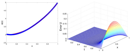
Figure 1. Exact (solid line) and restored (line with circles) diffusion coefficient $a\left(x\right)$ (left) and solution u (right), $\alpha =0.5$, ${\rho }_a=0.05$, ${\rho }_u=0.01$.

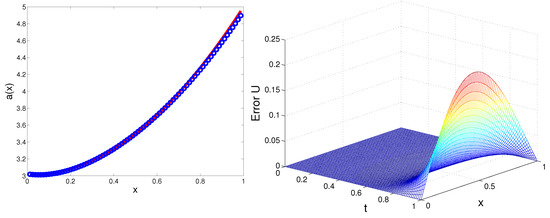
Figure 2. Exact (solid line) and restored (line with circles) diffusion coefficient $a\left(x\right)$ (left) and solution u (right), $\alpha =0.9$, ${\rho }_a=0.05$, ${\rho }_u=0.01$.

In Figure 3, we depict the exact and restored diffusion $a\left(x\right)$ for $N=M=80$, $\alpha =0.25$ and $\alpha =0.95$, ${\rho }_a=0.1$ and ${\rho }_u=0.05$. We observe that for both values of the fractional order, the accuracy of the restored function is very close.

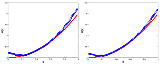
Figure 3. Exact (solid line) and restored (line with circles) diffusion coefficient $a\left(x\right)$, $\alpha =0.25$ (left) and $\alpha =0.95$ (right), ${\rho }_a=0.1$, ${\rho }_u=0.03$.

The results show that the main factor for the accuracy of the solution is the deviation of the measurements, rather than the fractional order.

Next, we take initial function, right-hand side

$$u_0\left(x\right)=2sin\left(\pi x\right),f(x,t)=5\left(\Gamma (1+{\alpha }_1)+\frac{\Gamma (1+2{\alpha }_1)}{\Gamma (1+{\alpha }_1)}{t}^{{\alpha }_1}+\frac{\Gamma (1+3{\alpha }_1)}{\Gamma (1+2{\alpha }_1)}{t}^{2{\alpha }_1}\right)sin\left(\pi x\right)$$

and generate perturbed data from (34), (35), replacing the exact solution u with a numerical solution of the direct problem, computed for the exact diffusion coefficient. Then, the solution of the discrete inverse problem U will be compared with the corresponding numerical solution of the direct problem. The computations are performed for $N=M=80$ and the same points of measurements as in previous test. On Figure 4 (left), we illustrate the impact of the fractional order on the accuracy for ${\rho }_a=0.1$, ${\rho }_u=0.08$. As before, we deduce that it is not so significant. On Figure 4 (right), we examine the impact of the perturbation on the accuracy for $\alpha =0.5$. We observe that the deviation has a larger impact on accuracy than the fractional order. On Figure 5, we plot the error of the solution for $\alpha =0.5$ and two sets of perturbation ${\rho }_a={\rho }_u=0.01$ and ${\rho }_a={\rho }_u=0.1$. In spite of the noise affecting the accuracy of the solution, it is evident that the precision of the solution is quite satisfactory when employing the recovered diffusion coefficient.

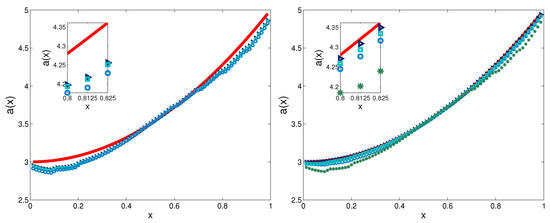
Figure 4. Dependence on the fractional order (left): exact (solid line) and restored diffusion coefficient $a\left(x\right)$, $\alpha =0.25$ (line with triangles), $\alpha =0.5$ (line with squares), $\alpha =0.95$ (line with circles), ${\rho }_a=0.1$, ${\rho }_u=0.08$; dependence on the perturbation (right): Exact (solid line) and restored diffusion coefficient $a\left(x\right)$, ${\rho }_a=0.01$, ${\rho }_u=0.01$ (line with triangles), ${\rho }_a=0.05$, ${\rho }_u=0.01$ (line with circles), ${\rho }_a=0.01$, ${\rho }_u=0.05$ (line with squares), ${\rho }_a=0.1$, ${\rho }_u=0.1$ (line with stars).

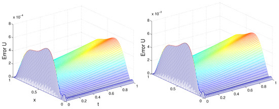
Figure 5. Error of the solution for ${\rho }_a={\rho }_u=0.01$ (left) and ${\rho }_a={\rho }_u=0.1$ (right).

The computational simulations, presented in this section to test the proposed approach are implemented by MATLAB^® R2022a.

8. Conclusions

In this paper, we have solved a single fractional parabolic integro-differential equation, derived by reducing a coupled fractional parabolic PDE-ODE system. First, we discussed the well-posedness of the Dirichlet problem and then we performed an analysis for stability and convergence of Alikhanov’s scheme [29]. We have developed an approach for numerical recovering of the space-dependent diffusion coefficient using a finite number of space points observations. We have experimentally illustrated the efficacy of the suggested method. The order of the fractional derivative does not significantly affect the results. The numerical tests with perturbed data showed the accurate recovery of the diffusion coefficient with a satisfactory error.

We intend to expand the investigation presented in this paper to other inverse problems of type [37,38,39,40,41,42] for one and multidimensional systems of fractional differential equations.

References

- Alaimo, G.; Piccolo, V.; Cutolo, A.; Deseri, L.; Fraldi, M.; Zingales, M. A fractional order theory of poroelasticity. Mech. Res. Commun. 2019, 100, 103395. [Google Scholar] [CrossRef]
- Alifanov, O.M.; Artioukhine, E.A.; Rumyantsev, S.V. Extreme Methods for Solving Ill-Posed Problems with Applications to Inverse Heat Transfer Problems; Begell House: Danbury, CT, USA, 1995. [Google Scholar]
- Armstrong, J.E.; Frind, E.O.; McClellan, R.D. Nonequilibrium mass transfer between the vapor, aqueous, and solid phases in unsaturated soils during vapor extraction. Water Resour. Res. 1994, 30, 355–368. [Google Scholar] [CrossRef]
- Burqan, A.; Shqair, M.; El-Ajou, A.; Ismaeel, S.M.E.; AlZhour, Z. Analytical solutions to the coupled fractional neutron diffusion equations with delayed neutrons system using Laplace transform method. AIMS Math. 2023, 8, 19297–19312. [Google Scholar] [CrossRef]
- Gao, G.; Zhan, H.; Feng, S.; Fu, B.; Ma, Y.; Huang, G. A new mobile-immobile model for reactive solute transport with scale-dependent dispersion. Water Resour. Res. 2010, 46, 1–16. [Google Scholar] [CrossRef]
- Goulart, A.G.; Lazo, M.J.; Suarez, J.M.S. A new parameterization for the concentration flux using the fractional calculus to model the dispersion of contaminants in the planetary boundary layer. Phys. A Stat. Mech. Appl. 2019, 518, 38–49. [Google Scholar] [CrossRef]
- Li, X.; Wen, Z.; Zhu, Q.; Jakada, H. A mobile-immobile model for reactive solute transport in a radial two-zone confined aquifer. J. Hydrol. 2020, 580, 124347. [Google Scholar] [CrossRef]
- Mahiudin, M.; Godhani, D.; Feng, L.; Liu, F.; Langrish, T.; Karim, M. Application of Caputo fractional rheological model to determine the viscoelastic and mechanical properties of fruit and vegetables. J. Postharvest Biol. Technol. 2020, 163, 111147. [Google Scholar] [CrossRef]
- Vougalter, V. Inverse problems for some systems of parabolic equations with coefficient depending on time. In Mathematical Methods in Modern Complexity Science; Springer International Publishing: Berlin/Heidelberg, Germany, 2021; pp. 189–197. [Google Scholar]
- Zhou, H.; Yang, S.; Zhang, S. Modeling non-darcian flow and solute transport in porous media with the caputo–fabrizio derivative. Appl. Math. Model. 2019, 68, 603–615. [Google Scholar] [CrossRef]
- Gyulov, T.B.; Vulkov, L.G. Reconstruction of the lumped water-to-air mass transfer coefficient from final time or time-averaged concentration measurement in a model porous media. In Proceedings of the 16th Annual Meeting of the Bulgarian Section of SIAM, Sofia, Bulgaria, 21–23 December 2021. [Google Scholar]
- Georgiev, S.; Vulkov, L. Numerical coefficient reconstruction of time-depending integer- and fractional-order SIR models for economic analysis of COVID-19. Mathematics 2022, 10, 4247. [Google Scholar] [CrossRef]
- Caputo, M.; Plastino, W. Diffusion in porous layers with memory. Geophys. J. Int. 2004, 158, 385–396. [Google Scholar] [CrossRef]
- Koleva, M.N.; Vulkov, L.G. Parameters Estimation in a Time-Fractiona Parabolic System of Porous Media. Fractal Fract. 2023, 7, 443. [Google Scholar] [CrossRef]
- Shen, S.; Weizhong Dai, W.; Cheng, J. Fractional parabolic two-step model and its accurate numerical scheme for nanoscale heat conduction. J. Comput. Appl. Math. 2020, 375, 112812. [Google Scholar] [CrossRef]
- Georgiev, S.; Vulkov, L. Parameters identification and numerical simulation for a fractional model of honeybee population dynamics. Fractal Fract. 2023, 7, 311. [Google Scholar] [CrossRef]
- Koleva, M.N.; Vulkov, L.G. Fast Positivity Preserving Numerical Method for Time-Fractional Regime-Switching Option Pricing Problem. In Advanced Computing in Industrial Mathematics. BGSIAM 2020; Studies 295 in Computational Intelligence; Georgiev, I., Kostadinov, H., Lilkova, E., Eds.; Springer: Cham, Switzerland, 2023; Volume 1076. [Google Scholar]
- Tarasov, V.E. (Ed.) Special Issue “Fractional Calculus in Economics and Finance”. Fractal Fract. 2018. Available online: https://www.mdpi.com/journal/fractalfract/special_issues/Fractional_Calculus_Economics_Finance (accessed on 26 June 2023).
- Kandilarov, J.; Vulkov, L. Determination of concentration source in a fractional derivative model of atmospheric pollution. AIP Conf. Proc. 2021, 2333, 090014. [Google Scholar] [CrossRef]
- Liu, W.; Li, G.; Jia, X. Numerical simulation for a fractal MIM model for solute transport in porous media. J. Math. Res. 2021, 13, 31–44. [Google Scholar] [CrossRef]
- Jovanović, B.S.; Vulkov, L.G.; Delić, A. Boundary value problems for fractional PDE and their numerical approximation. In Numerical Analysis and Its Applications; Lecture Notes in Computer Science; Springer: Berlin/Heidelberg, Germany, 2013; Volume 8236, pp. 38–49. [Google Scholar]
- Kilbas, A.A.; Srivastava, H.M.; Trujillo, J.J. Theory and Applications of Fractional Differential Equations; North-Holland Mathematics Studies; Elsevier: Amsterdam, The Netherlands, 2006; Volume 204. [Google Scholar]
- Podlubny, I. Fractional Differential Rquations; Academic Theory and Applications of Fractional Differential Equations; Elsevier: Amsterdam, The Netherlands, 1998. [Google Scholar]
- Gyulov, T.; Vulkov, L. Gradient Optimization in Reconstruction of the Diffusion Coefficient in a Time Fractional Integro-Differential Equation of Pollution in Porous Media. In Modelling and Development of Intelligent Systems MDIS; Communications in Computer and Information Science; Simian, D., Stoica, L.F., Eds.; Springer: Cham, Switzerland, 2022; Volume 1761. [Google Scholar]
- Wei, T.; Xian, J. Variational method for a backward problem for a time-fractional diffusion equation. ESAIM M2AN 2019, 53, 1223–1244. [Google Scholar] [CrossRef]
- Alikhanov, A.A. A priori estimates for solutions of boundary value problems for fractional-order equations. Differ. Equ. 2010, 46, 660–666. [Google Scholar] [CrossRef]
- Hasanov, A.H.; Romanov, V.G. Introduction to Inverse Problems for Differential Equations; Springer: Cham, Switzerland, 2017. [Google Scholar] [CrossRef]
- Samarskii, A.A. The Theory of Difference Schemes; Marcel Dekker: New York, NY, USA, 2001. [Google Scholar]
- Alikhanov, A.A. A new difference scheme for the time fractional diffusion equation. J. Comput. Phys. 2015, 280, 424–438. [Google Scholar] [CrossRef]
- Li, D.; Liao, H.-L.; Sun, W.; Wang, J.; Zhang, J. Analysis of L1 Galerkin FEMs for time-fractional nonlinear parabolic problems. Commun. Comput. Phys. 2018, 24, 86–103. [Google Scholar] [CrossRef]
- Chavent, G. Nonlinear Least Squares for Inverse Problems: Theoretical Foundations and Step-by-Step Guide for Applications; Scientific Computation; Springer: Dordrecht, The Netherlands, 2010. [Google Scholar] [CrossRef]
- Hanke, M. Conjugate Gradient Type Methods for Ill-Posed Problems, 1st ed.; Chapman and Hall/CRC: New York, NY, USA, 1995. [Google Scholar]
- Vabishchevich, P.N.; Denisenko, A.Y. Numerical methods for solving the coefficient inverse problem. Comput. Math. Model. 1992, 3, 261–267. [Google Scholar] [CrossRef]
- Fletcher, R.; Reeves, C.M. Function minimization by conjugate gradients. Comput. J. 1964, 7, 149–154. [Google Scholar] [CrossRef]
- Fakhraie, M.; Shidfar, A.; Garshasbi, M. A computational procedure for estimation of an unknown coefficient in an inverse boundary value problem. Appl. Math. Comput. 2007, 187, 1120–1125. [Google Scholar] [CrossRef]
- Samarskii, A.A.; Vabishchevich, P.N. Numerical Methods for Solving Inverse Problems in Mathematical Physics; De Gruyter: Berlin, Germany, 2007; 438p. [Google Scholar]
- Durdiev, D.K.; Zhumaev, Z.Z. One-dimensional inverse problems of finding the kernel of integrodifferential heat equation in a bounded domain. Ukr. Math. J. 2022, 73, 1723–1740. [Google Scholar] [CrossRef]
- Li, Z.; Yamamoto, M. Uniqueness for inverse problems of determining orders of multi-term time-fractional derivatives of diffusion equations. Appl. Anal. 2015, 94, 570–579. [Google Scholar] [CrossRef]
- Li, Z.; Huang, X.; Yamamoto, M. A stability result for the determination of order in time-fractional diffusion equations. J. Inverse -Ill-Posed Probl. 2020, 28, 379–388. [Google Scholar] [CrossRef]
- Sun, L.; Wei, T. Identification of the zeroth-order coefficient in a time fractional diffusion equation. Appl. Numer. Math. 2017, 111, 160–180. [Google Scholar] [CrossRef]
- Tikhonov, A.; Arsenin, V. Solutions of Ill-Posed Problems; V. H. Winston: Winston, WA, USA, 1977. [Google Scholar]
- Li, Z.; Yamamoto, M. Inverse Problems of Determining Coefficients of the Fractional Partial Differential Equations; Kochubei, A., Luchko, Y., Eds.; Volume 2 Fractional Differential Equations; De Gruyter: Berlin, Germany; Boston, MA, USA, 2019; pp. 443–464. [Google Scholar]
Disclaimer/Publisher’s Note: The statements, opinions and data contained in all publications are solely those of the individual author(s) and contributor(s) and not of MDPI and/or the editor(s). MDPI and/or the editor(s) disclaim responsibility for any injury to people or property resulting from any ideas, methods, instructions or products referred to in the content. |
© 2023 by the authors. Licensee MDPI, Basel, Switzerland. This article is an open access article distributed under the terms and conditions of the Creative Commons Attribution (CC BY) license (https://creativecommons.org/licenses/by/4.0/).