Daughter Coloured Noises: The Legacy of Their Mother White Noises Drawn from Different Probability Distributions

Abstract

White noise is fundamentally linked to many processes; it has a flat power spectral density and a delta-correlated autocorrelation. Operators acting on white noise can result in coloured noise, whether they operate in the time domain, like fractional calculus, or in the frequency domain, like spectral processing. We investigate whether any of the white noise properties remain in the coloured noises produced by the action of an operator. For a coloured noise, which drives a physical system, we provide evidence to pinpoint the mother process from which it came. We demonstrate the existence of two indices, that is, kurtosis and codifference, whose values can categorise coloured noises according to their mother process. Four different mother processes are used in this study: Gaussian, Laplace, Cauchy, and Uniform white noise distributions. The mother process determines the kurtosis value of the coloured noises that are produced. It maintains its value for Gaussian, never converges for Cauchy, and takes values for Laplace and Uniform that are within a range of its white noise value. In addition, the codifference function maintains its value for zero lag-time essentially constant around the value of the corresponding white noise.

1. Introduction

Noise is an inherent property of any physical system. The perception of noise, whether constructive or destructive, differs from one scientific field to another. In information theory, noise stands for whatever masks the information content of a signal; noise is a nuisance that should be eliminated or minimised as much as possible in order to detect a signal. On the contrary, in biology, physics, chemistry, and neuroscience, noise refers to background fluctuations that can interfere with the system itself. The constructive role of noise in the last few decades has been pointed out, for example, in stochastic resonance or Brownian ratchets, where additive or multiplicative noises drive the system behaviour, even increasing its efficiency [1].

White noise is probably the most commonly used descriptor for fluctuations in physical, chemical, and biological systems. It typically represents thermal effects at equilibrium. A random process is “white noise”, when the distribution of its power spectrum density (PSD) in the frequency domain is flat across all available frequencies. In addition to that, the auto-correlation function (ACF) of white noise is delta-correlated. In discrete space, a white noise sequence has the form of time-ordered and hierarchically distributed, uncorrelated random variables. A sequence formed by independent and identically distributed (i.i.d.) random variables whose values are drawn from a probability distribution function (PDF) is a white noise. The opposite statement, that white noise is a collection of i.i.d. random variables, is not necessarily true. Numerically, white noise is created as a sequence of uncorrelated pseudorandom numbers repeated only after a significantly large number of steps. The i.i.d. values of white noise can be uniformly or normally distributed around a zero mean value. They can also satisfy various PDFs.

As opposed to systems at equilibrium, where white noise can be used to encode all fast-decaying interactions, systems close to or far from equilibrium are better described by coloured noises. The colour of a noise is defined by the value of the slope of PSD of the linear regression on the log–log scale. If the PSD of a noise scales as a power law of the frequency, f, that is, $1/f^{\beta }$, then the value of $\beta$ classifies the colour. It is purple for $\beta =-2$, blue for $\beta =-1$, white for $\beta =0$, pink for $\beta =1$, red for $\beta =2$, and black for $\beta >2$. Coloured noises can be associated with the presence of a drift term or a gradient, with the presence of a restoring mechanism, or with a synergic action or even brain functioning. For example, red noise has long been linked to the motion of molecules and particles (Brownian motion) [2,3,4,5]. A pink or flickering noise can drive animal populations and result in synchronization and co-operativity [6]. Black noises are associated with the frequency of natural disasters [7]. In recent years, coloured noises have therefore acquired increasing importance. They can either deliver information related to the environment where a random process takes place or they can drive a system. The latter requires the formation of a memory, that is, the process should follow up to a point or trend, which can either be persistent or anti-persistent. Persistence is accompanied by a slowly varying ACF, thus reflecting the trend of a process that will likely follow its latest values. On the other hand, anti-persistence points to a process that reverses itself more often than white noise, and the ACF takes negative values.

Coloured noises can be numerically produced starting from a white noise sequence through the action of a proper operator (filter). There are various algorithms available to create coloured noises, and it is important to distinguish between those working in the time domain and those in the frequency domain. Auto-regressive approaches [8,9], physics-inspired algorithms based on Langevin-type equations [10,11], and Fractional Calculus [12] work in the time domain. In the frequency domain, fast-Fourier transform (FFT)-based algorithms are commonly used [13,14]. All algorithms convert the white noise input into coloured noise output. This means that under the same transformation, white noises (mother processes) drawn from various probability distributions “give birth” to coloured noises (daughter processes), whose colour is the same regardless of the initial distribution of white noise. The question is whether and to what extent the daughter process retains some of the properties of the mother process.

The colour (that is the spectral exponent, $\beta$) as an index for describing a random process is second order statistics [15,16], and accordingly it roughly describes a random process around its mean and variance, while the mean necessarily does not exist for a plethora of random processes. A classification based only on the colour code cannot distinguish daughter processes coming from different mother processes, and thus a study limited to the PSD is not able to shed light on differences in coloured noises produced by different white noise distributions. The auto-correlation function (ACF) is a widely used metric for analyzing stochastic process characteristics. ACF is second-order statistics, just like PSD; it tells us whether a noise is persistent or anti-persistent (i.e., the kind of memory it retains). Apart from ACF and PSD, fractal dimension (FD) [17], Hurst exponent, (H), and generalised moments method (GMM) have been used to characterise noise properties [18]. In general, FD and H values describe a random process around its mean and are precise for monofractal processes. On the other hand, GMM can accurately describe the properties of non-stationary processes, while for stationary processes, GMM returns a zero Hurst exponent, and the evaluation of the latter goes through Rescale range analysis (R/S); see details in [19].

In order to detect mother process imprints on the daughter ones, we estimate the kurtosis of each produced coloured noise and compare it to the value of the kurtosis of the corresponding white noise. The value of the kurtosis of data series formed by the time average mean square displacement of single trajectories has been used to classify the input trajectories either as ergodic or not [20,21]. This parameter is called the ergodicity breaking parameter (EB), and it has become a widely used measure to quantify fluctuations from trajectory to trajectory [22]. Kurtosis, however, does not always exist since there are distributions with non-existent moments; for example, the first moment is not defined for the Cauchy distribution, and the higher moments diverge. To overcome this obstacle, we use the codifference function (CD) [23]. CD makes use of the characteristic function and thus it always exists.

In this work, we create symmetric alpha stable (SaS) white noises, which draw values from either a Gaussian (G), a Laplace (L), a Cauchy (C), or a Uniform (U) distribution. For each one of them, we create coloured noises with a spectral exponent, $\beta \in [-1,1)$. Two techniques are used, namely, fractional calculus (FC), operating in the time domain, and spectral processing (SP), operating in the frequency domain. Each produced noise is characterized in terms of ACF, PSD, CD, and kurtosis. We show that ACF and PSD cannot discriminate between coloured noises produced by different white noise distributions. On the other hand, kurtosis and CD can be used as indicators of the mother process traits that have persisted in the daughter process.

2. White Noises and Probability Distributions

Let $X_t$ be an i.i.d. random variable drawing values from a probability distribution $P(X;\mu ,\sigma )$. A sequence of time-ordered events, $X_{t_i}$, with $i=1,2,3,\cdots ,n$, and $0<t_1<t_2<t_3<\cdots <t_n$ defines a random process. Such a process is called white noise and it is strictly stationary, as all i.i.d. random processes are. Strictly stationary means that the statistical properties of a process do not change over time, or in other words, the distribution of a number of random variables is the same as we shift them along the time indexed axis. Strictly stationary does not imply the existence of finite moments. Random processes with a constant mean, a finite second moment, and cross-correlation that depends only on the time lag are called weak stationary. Gaussian distributed i.i.d. random variables fulfill the criteria of both strict and weak stationary. It is important to notice that neither strict nor weak stationary imply one another.

Let two i.i.d. random variables have a common distribution, then if any linear combination of the two has the same distribution up to location and scale parameters then the distribution is called stable (unchanged shape). Stable distributions is an important class of probability distributions with interesting properties [24]. Stable distributions are also known as $\alpha$-stable Lévy distributions. An $\alpha$-stable distribution, $L_{\alpha }(X;\mu ,b,\sigma )$, requires four parameters for its complete description and is defined through its characteristic function, $CF\left(k\right)$. $CF\left(k\right)=P(k;\alpha ,b,\mu ,\sigma )={\int }_{-\infty }^{\infty }{e}^{ikX}P(X;\alpha ,b,\mu ,\sigma )$ is the Fourier transform of $P(X;\alpha ,b,\mu ,\sigma )$, and it always exists for any real-valued random variable as opposed to the moment’s generating function. The $CF\left(k\right)$ of an $\alpha$-stable distribution reads [25]

$$ln\left(C{F}_{\alpha }\left(k\right)\right)=\left\{\begin{array}{cc}\hfill -{\sigma }^{\alpha }{\left|k\right|}^{\alpha }\left\{1-ibsign\left(k\right)tan\left(\frac{\pi \alpha }{2}\right)\right\}+i\mu k\hfill & \hfill \alpha \ne 1\hfill \\ \hfill -\sigma \left|k\right|\{1+ibsign\left(k\right)\frac{2}{\pi }ln|k\left|\right\}+i\mu k\hfill & \hfill \alpha =1\hfill \end{array}\right.$$

(1)

where $\alpha \in (0,2]$ is the index of stability or characteristic exponent, $b\in [-1,1]$ is a skewness parameter, $\sigma \in R_{+}^{*}$ is a scale parameter, and $\mu \in R$ is a location parameter or mean. For $b=0$, Equation (1) returns the characteristic function of the stretched exponential centred around its mean, $\mu$. For $\alpha <2$, the distribution has undefined variance, while for $\alpha \le 1$ it has undefined mean. For $\alpha =2$ and for $\alpha =1$, Equation (1) returns the Gaussian and the Cauchy distributions, respectively, which read

$$L_2(X;\mu ,0,\sigma )=P_G(x;\mu ,\sigma )=\frac{1}{\sqrt{2\pi }\sigma }{e}^{-\frac{{(x-\mu )}^2}{2{\sigma }^2}}$$

(2)

and

$$L_1(X;\mu ,0,\sigma )=P_C(x;\mu ,\sigma )=\frac{1}{\pi \sigma }\frac{{\sigma }^2}{{(x-\mu )}^2+{\sigma }^2}$$

(3)

Mean, variance, skewness and kurtosis are expressed by the moments of the probability distribution up to 4th order. The qth order integer moment with $q\in {\mathbb{Z}}_{+}$ is derived directly from Equation (1) as

$$S\left(q\right)={(-i)}^q\frac{{\partial }^{q}CF\left(k\right)}{\partial k^q}{|}_{k=0}$$

(4)

(Alternatively, the moments can be obtained directly from the integral $S\left(q\right)=<X^q>={\int }_{-\infty }^{\infty }{X}^{q}P\left(X\right)dX$, when the pdf $P\left(X\right)$ is known).

Equation (4) can be generalized to also include fractional order moments and reads [26]

$$S(q+m)=\frac{1}{cos\left(\frac{(q+m)\pi }{2}\right)}\mathbb{R}\left[\frac{{\partial }^{q+m}CF\left(k\right)}{\partial k^{q+m}}{|}_{k=0}\right]$$

(5)

where $q\ge 0\in {\mathbb{Z}}_{+}$, $0<m<1$, and $\mathbb{R}$ stands for the real part of the complex number. Having Equation (5) as a starting point, one can obtain absolute moments centered around the mean; see, for example, [27].

Geometric stable laws constitute a class of limiting distributions of appropriately normalized sums of i.i.d. random variables [28]. $C{F}_G\left(k\right)$ is the characteristic function of a geometric stable distribution if and only if it is connected to the characteristic function of an $\alpha$-stable distribution, $C{F}_{\alpha }\left(k\right)$, through the relation

$$C{F}_G\left(k\right)=\frac{1}{1-ln\left(C{F}_{\alpha }\left(k\right)\right)}={\int }_{-\infty }^{\infty }{\left[C{F}_{\alpha }\left(k\right)\right]}^u{e}^{-u}du$$

(6)

with stability index, $\alpha$, mean or location parameter, $\mu$, scale parameter, $\sigma$, and asymmetry parameter, b, are used to describe a geometric stable distribution. For $\alpha =2$, $\mu =0$, $b=0$, and scale parameter $\sqrt{2}\sigma$, Equation (6) gives the characteristic function of the standard Laplace distribution, whose analytic form reads

$$P_L(x;\mu ,\sigma )=\frac{1}{2\sigma }{e}^{-}\frac{|x-\mu |}{\sigma }$$

(7)

In addition, Equation (7) for $\sigma =1$ returns the classical Laplace distribution whose PDF can be expressed as addition or multiplication of i.i.d. random processes; see Table 2.3 in [29].

Finally, we also use the uniform distribution (U) with pdf

$$P_U(x;a,b)=\left\{\begin{array}{cc}\frac{1}{b-a}\hfill & \hfill a\le x\le b\hfill \\ \hfill 0\hfill & \hfill \mathrm{otherwise}\hfill \end{array}\right.$$

(8)

with a and b being the values range of the distribution. For $a=-\sqrt{3}$ and $b=\sqrt{3}$, Equation (8) returns the uniform (U) distribution with zero mean and variance 1. The U-distribution is used as an auxiliary one for constructing L and C distributions in discrete space see below.

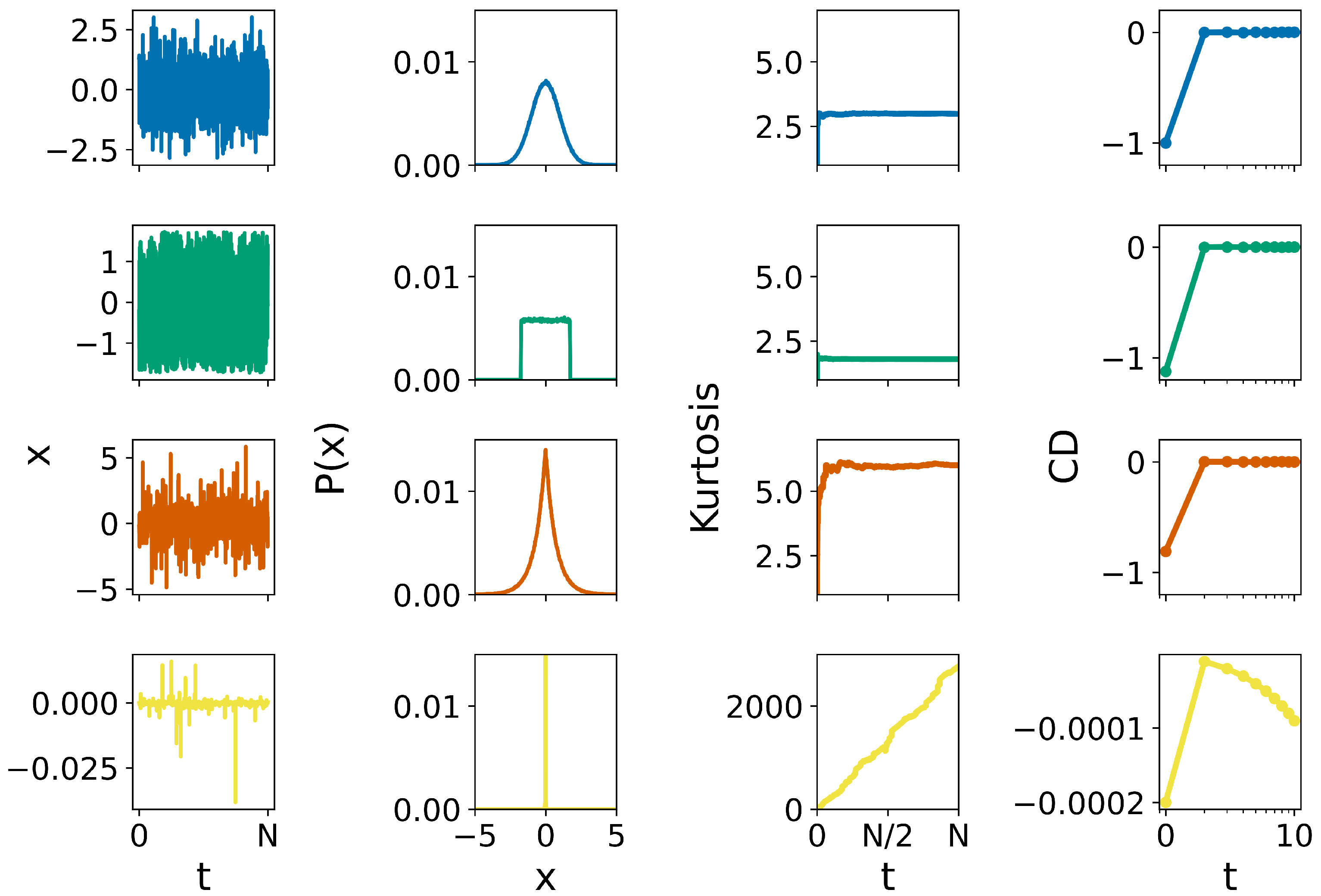
The discrete white noise time series shown in Figure 1 were generated using Matlab [30]. Technically speaking, the function $\mathit{rand}$ of [30] has been used to create uniformly distributed random numbers, $x_U\in (0,1)$. The function $\mathit{randn}$ of [30], which is based on the Box–Muller algorithm [31] as $x_G=randn=\sqrt{-ln\left(x_U^1\right)}cos\left(2\pi x_U^2\right)$, where $x_U^1$ and $x_U^2$ are two uniformly distributed random numbers in the range (0,1) [32], has been used to produce Gaussian distributed random numbers. A Laplace (L) distributed white noise sequence is generated as the ratio of two uniformly distributed random numbers, $x_U^1$ and $x_U^2$, taken as values in the range (0,1), $x_L=ln(\frac{x_U^1}{x_U^2})$ [33]. A Cauchy (C) white noise distribution is generated as $x_C=tan\left(\pi (x_U-0.5)\right)$, where $x_U$ is uniformly distributed random number in (0,1) [34]. Notice also that a Cauchy distribution can be constructed as the ratio of two i.i.d. discrete random variables with values drawn from the Gaussian distribution. All white noise sequences used in this work were shifted properly to have a zero mean and unitary variance. The length of each of them was set to $N={10}^6$ steps, and for the sake of simplicity, we convert steps/realizations to time steps (arbitrary units). Codifference is estimated as a function of the time lag, whose values fall within the range $[0,N/100]$, and its value is estimated from Equations (A6) and (A7); see Appendix A.

Typical statistical measures of classifying time series are the autocorrelation function (ACF), power spectral density (PSD), mean square displacement (MSD), and its generalization (generalized moments method, GMM), which includes moments smaller and higher than two, including also fractional moments [18]. For all white noises used in this study, ACF is by definition delta-correlated, and thus no distinction can be made based on it. Similar, PSD is flat for all noises, and GMM depends on ${\sigma }^q$, q being the order of the moment, and only the prefactor changes from one white noise to another; see the analytical forms of the absolute central moments in

Table 1. Characteristic Function (CF), absolute central moments ($S\left(q\right)$), mean, variance (var), skewness (Sk), and Kurtosis (Ku) for Uniform (U), Gaussian (G), Laplacian (L), and Cauchy (C) i.i.d. random variables. Variance, skewness, and kurtosis can be obtained from the absolute central moments. In addition, for $q\ge 1$ all moments of the Cauchy distribution are either undefined or go to infinity; however, after a suitable renormalization, for example, dividing each component of the probability distribution by its highest value, all the moments of a Cauchy distribution may exist.

	$\mathbf{CF}\left(\mathit{k}\right)$	$\mathit{S}\left(\mathit{q}\right)={|\mathit{x}-\mathit{\mu }|}^{\mathit{q}}$	mean	var	Sk	Ku
U	$-i\frac{e^{ikb}-e^{ika}}{k(b-a)}$	$\frac{(1+{(-1)}^q){(b-a)}^q}{2^{q+1}(q+1)}$	$\frac{b+a}{2}$	$\frac{{(b-a)}^2}{12}$	0	1.8
G	$e^{ik\mu -\frac{k^2{\sigma }^2}{2}}$	$\frac{2^{q/2}}{\sqrt{\pi }}\Gamma \left(\frac{q+1}{2}\right){\sigma }^q$	$\mu$	${\sigma }^2$	0	3
L	$\frac{e^{i\mu k}}{1+{\sigma }^2{k}^2}$	$\Gamma (q+1){\sigma }^q$	$\mu$	$2{\sigma }^2$	0	6
C	$e^{i\mu k-\sigma \left|k\right|}$	${\sigma }^{q}Sec\left(\frac{\pi q}{2}\right),-1<q<1$	undefined	∞	∞	∞

. In addition, by construction, the produced white noises are of symmetric $\alpha$-stable sequences (SaS), and accordingly, skewness is zero. Kurtosis provides the first indication regarding the differences between the white noise sequences [35]. The values of the kurtosis for the different white noises shown in Figure 1 are exactly in line with theory; see Table 1. A standard Gaussian white noise is characterized by a kurtosis of 3 and has a mesokurtic distribution. Distributions with kurtosis values greater than 3 are named leptokurtic, while PDFs with kurtosis values smaller than 3 are said to be platykurtic. In this frame, Laplace and Cauchy white noise are leptokurtic, while Uniform white noise is platykurtic. The codifference function for each white noise is also shown in Figure 1. The definitions for the codifference function are given in Appendix A; see Equations (A5)–(A7). For Gaussian white noise, the codifference function is equal to $CD(G\left(t\right),G\left(s\right))=-{\sigma }^2$ for $t=s$ and zero otherwise. Equation (A8), and the result depicted in Figure 1 is in perfect agreement with theory. Equation (A12) provides the codifference function for Cauchy white noise, and is zero, in agreement with our findings presented in Figure 1. The codifference function takes the values $-1$ for Gaussian, $-0.81$ for Laplace, and $-1.12$ for Uniform; see also

Table 2. Codifference values for lag-time $\tau =0$, $CD(1,-1;0)$, obtained from numerical simulations of the mother white noises, namely, Gaussian, Laplace, and Uniform, as well as for all their daughter coloured noises ($\beta =[-1,0.75]$), produced either with FC or with SP. For Cauchy white and coloured noises, CD $(\tau =0)=0$.

$\mathit{\beta }$	$-1$	$-0.75$	$-0.50$	$-0.25$	0	0.25	0.50	0.75
Gaussian					$-1.0$
FC	$-1.0$	$-1.0$	$-1.0$	$-1.0$		$-1.0$	$-1.0$	$-1.0$
SP	$-1.0$	$-1.0$	$-1.0$	$-1.0$		$-1.0$	$-1.0$	$-1.0$
Laplace					$-0.81$
FC	$-0.87$	$-0.85$	$-0.83$	$-0.82$		$-0.82$	$-0.86$	$-0.92$
SP	$-0.84$	$-0.83$	$-0.82$	$-0.81$		$-0.82$	$-0.84$	$-0.90$
Uniform					$-1.12$
FC	$-1.08$	$-1.09$	$-1.10$	$-1.12$		$-1.12$	$-1.09$	$-1.04$
SP	$-1.09$	$-1.10$	$-1.11$	$-1.12$		$-1.12$	$-1.09$	$-1.05$

and discussion in Appendix A. Given that the codifference provides the similarity of the bulk of the distribution and has a value of $-1$ for Gaussian noise, we expect that this value will be smaller in absolute value for Laplace white noise (less similarity) and higher in absolute value for Uniform white noise (higher similarity).

Table 1 shows the absolute moments, the mean, the variance, the skewness, and the kurtosis for Gaussian, Laplace, Cauchy, and Uniform white noise distributions. Notice that the Cauchy distribution, Equation (3), has an undefined first moment and non-converging second moment. However, we can form white noise discrete distributions that have a constant mean and a time-dependent variance, which draw values from a Cauchy distribution by imposing a kind of truncation.

3. Generating $\alpha$- and Geometric Stable Noises in Discrete Space: Time and Frequency Domain Techniques

The white noise sequences of the previous section are the mother processes on which the action of the proper operator will create new time sequences, or daughter processes. The goal is to ascertain which characteristics of the mother process and to what extent they are carried over into the daughter process. We use two distinct operators: fractional calculus (FC), which operates in the time domain, and spectral processing (SP), which operates in the frequency domain.

3.1. Fractional Calculus (FC)

When white noise is integrated or differentiated in the time domain, red ($\beta =2$) and purple ($\beta =-2$) noises are produced, respectively. The operator (derivative/integral) can be extended to include non-integer orders, fractional calculus (FC) [36,37], and accordingly various colours may be produced from its action on a white noise sequence. The Riemann–Liouville fractional integral of order $\nu$ on a white noise reads

$${}_{t_0}{D}_t^{-\nu }w\left(t\right)=\frac{1}{\Gamma \left(\nu \right)}{\int }_{t_0}^t{(t-\tau )}^{\nu -1}w\left(\tau \right)d\tau =Y_{\beta }\left(t\right)$$

(9)

and we limit $\nu \in [0,1]$ for this work. Equation (9) also provides the fractional derivative of a white noise sequence, since fractional derivatives are defined through fractional integrals. Given that limit $\nu \in [0,1]$, a fractional derivative of order $\nu$ reads

$${}_{t_0}{D}_t^{\nu }w\left(t\right)={}_{t_0}{D}_t\times {}_{t_0}{D}_t^{-(1-\nu )}w\left(t\right)=\frac{d}{dt}\frac{1}{\Gamma (1-\nu )}{\int }_{t_0}^t{(t-\tau )}^{-\nu }w\left(\tau \right)d\tau =Y_{\beta }\left(t\right)$$

(10)

For integer $\nu$, Equations (9) and (10) return classical integration, derivation. The order of the fractional integration, differentiation is related to the power spectral exponent, $\beta$, of the coloured noise $Y_{\beta }\left(t\right)$, $\nu =\beta /2$. For $\nu =1$ and $\nu =1/2$, fractional integration of white noise returns red or Brownian noise and pink, respectively (correlated noises), while fractional differentiation of white noise delivers purple and blue noise, respectively, anti-correlated noise. Fractional derivatives/integrals are non-local operators [36,38,39] and thus can model memory effects whose implications modify properties of a physical system.

We use the Grunwald–Letnikov (GL) definition for the discrete implementation of FC [40]. Alternative definitions of fractional derivatives and integrals, such as Riemann–Liouville, Caputo, etc., could be used [41,42]. The GL left-sided definition of fractional derivative reads [42]

$${}_a{D}_t^{\nu }w\left(t\right)=\underset{h\to 0}{lim}\frac{1}{h^{\nu }}\sum _{j=0}^{⌊\frac{t-a}{h}⌋}{(-1)}^j\frac{\Gamma (\nu +1)}{\Gamma (j+1)\Gamma (\nu -j+1)}w(t-jh)$$

(11)

where $a\in R$ is constant and expresses a limit value, h is the discretization step, $⌊\frac{t-a}{h}⌋$ is the floor function, and $\Gamma \left(\right)$ is Euler’s Gamma function. Fractional integration and derivation were implemented in Matlab code [30].

3.2. Spectral Processing Method (SP)

Coloured noises can be produced by the spectral processing, frequency domain, of a white noise sequence. The algorithm is based on transforming a time series of white noise into the frequency domain, processing it spectrally, and then transforming it back into the time domain [14,43]. The algorithm consists of the following steps:

• Let N be the length/number of points of the sequence,
• Generate a pseudo-random white noise vector, $w\left(t\right)$, with $t=1,2,...,N$ sampled from a given probability distribution (U, G, L or C).
• Fast Fourier Transform of the white noise vector to $W\left(f\right)=FFT\left(w\right)$.
• Multiply the complex spectral coefficients of the white noise by h, $W^{\prime }\left(f\right)=W\left(f\right)f^h$, where $h=\beta /2$ and $\beta$ is the classifier of the colours.
• Back Fast Fourier transform of the spectral coefficients to obtain the coloured noise, $y\left(t\right)=IFFT(W’(f\left)\right)$.

Fractional coloured noises have been created using spectral processing with Matlab code [30].

4. Results and Discussion

Each white noise sequence depicted in Figure 1 is subject to the action of both fractional calculus (FC) and spectral processing (SP), and seven coloured sequences for each operator are produced. Therefore, each white noise (mother process) yields 14 daughter processes (7 with FC and 7 with SP), each of length $N={10}^6$. In total, we generate $4\times 14$ = 56 new sequences, which we analyze.

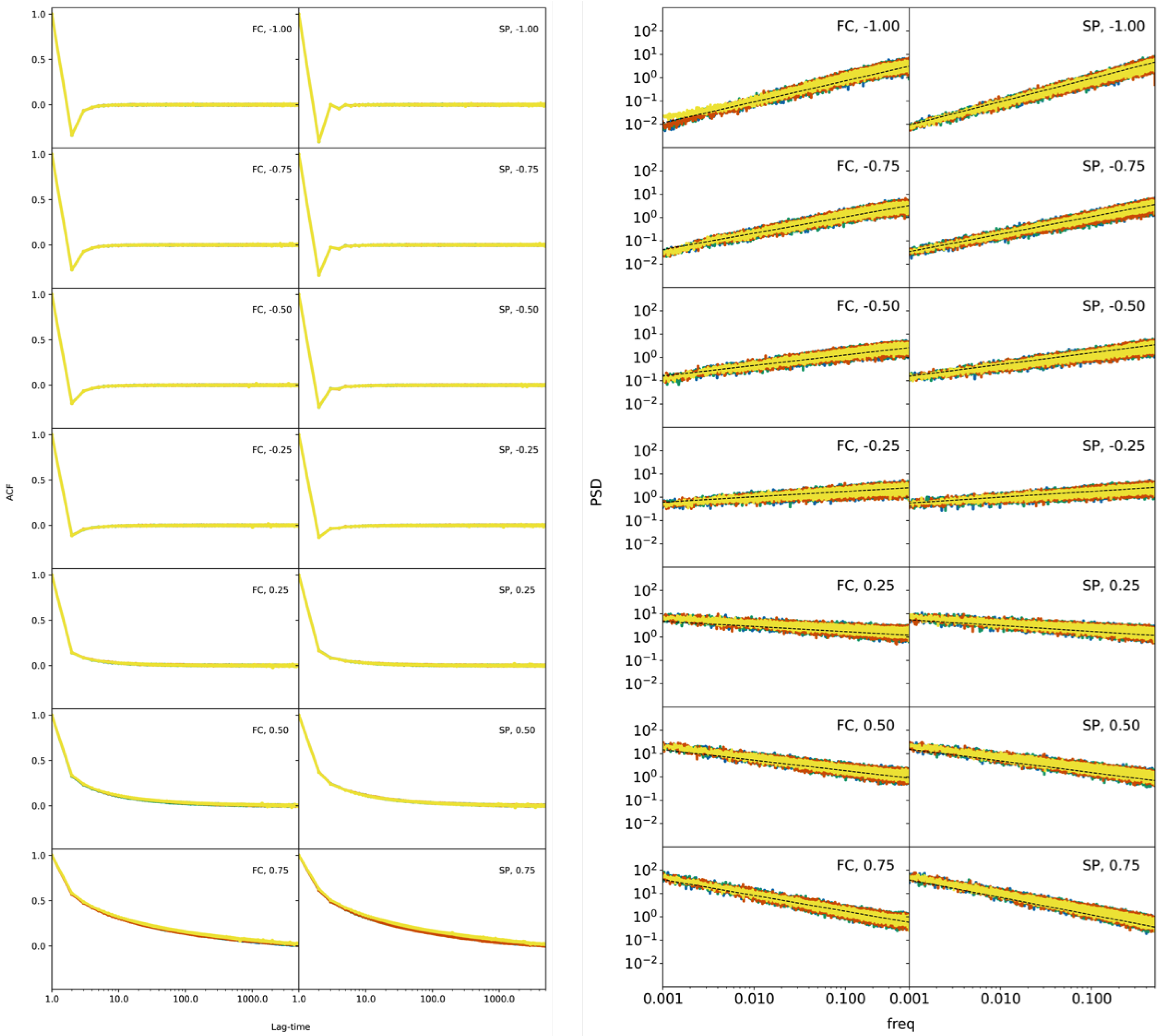
ACFs for daughter processes derived from the various white noises (G, L, C, and U) are essentially identical when a colour is used for comparative analysis (see Figure 2), and yet, the operator involved in the creation of each daughter process has no significant impact on the sequence that is produced in terms of this property. In addition, ACFs display the fundamental characteristics of the generated noises, i.e., correlated (smoother trajectories) and anti-correlated (rough trajectories). Contrary to non-vanishing ACFs for $0<\beta <1$, which indicate correlation, the small negative part of ACFs for $-1\le \beta <0$ highlights processes that are anti-correlated. Notice also that the effects of correlation, long tails, and anti-correlation, deeper minima, are stronger the higher the absolute value of $\beta$.

The PSDs do not distinguish between noise sequences of the same colour generated by various white noise distributions (G, L, C, and U). Actually, as it should be, the slope of the PSDs in log–log linear regression is maintained constant for at least four orders of magnitude, and its value relates to a particular colour. PSDs produced by the SP present some differences with respect to those produced by the FC. The SP method exerts a “brutal force” on the flat spectrum of white noise and reverts it by a given slope (colour), and thus all data points fit well into a linear regression on a log–log scale (see Figure 2). Instead, FC creates a memory that does not last for ever, and thus, in the long-time limit, this memory is washed out, and the spectrum in this region looks flat, retaining properties of the mother process from which it came. In addition, it has been noted that spectral methods accurately predict the scaling of synthetic time series produced in the frequency domain, while for those produced in the time domain, half of the spectra estimates deviate significantly for the nominal value of the scaling exponent [44].

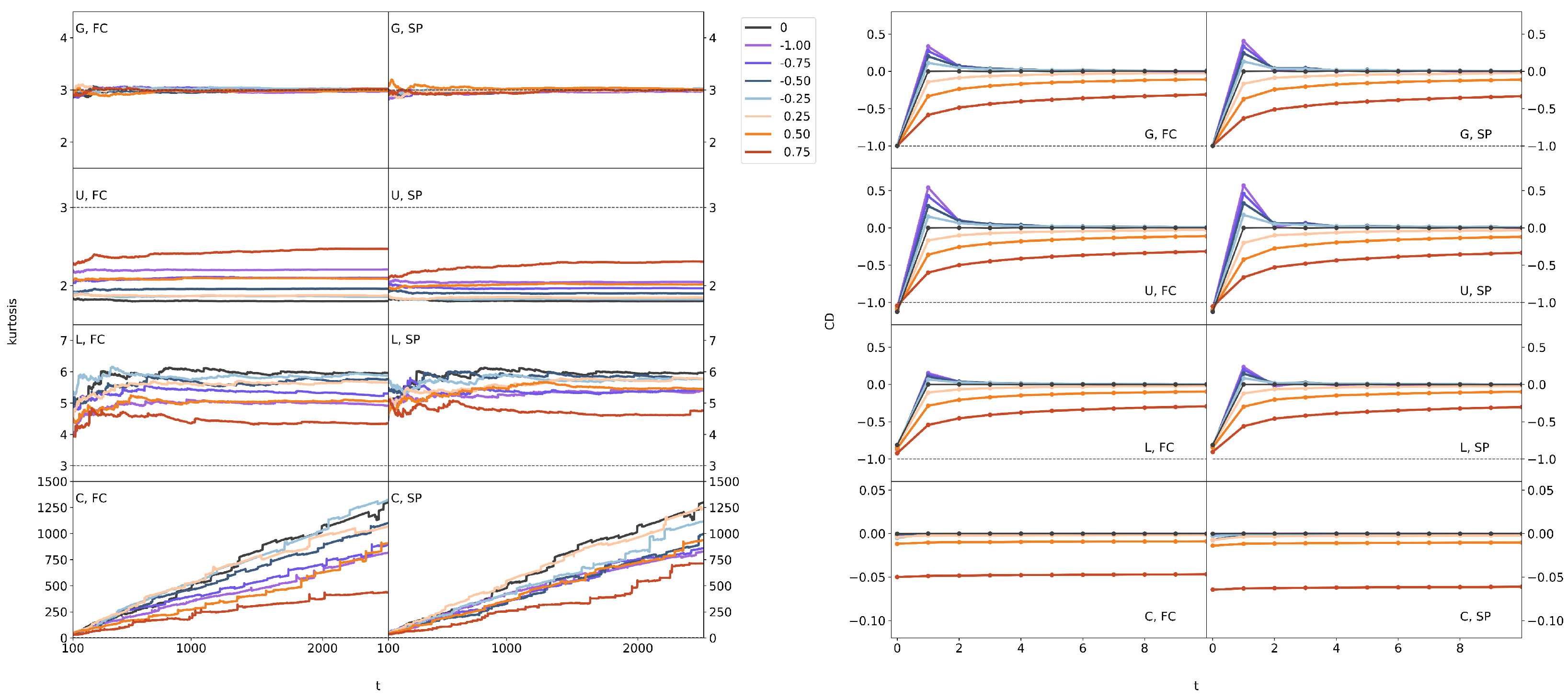
The first proof of discrimination between noises of the same colour producing white noise sampled from different PDFs is provided by kurtosis. The value of kurtosis for mother processes is equal to 3 for Gaussian, 6 for Laplace, and 1.8 for Uniform, and it is very large for Cauchy white noise (see Figure 1). Remarkably, daughter processes of the same colour but generated from different mother processes (i.e., different PDFs) differ (see Figure 3). Gaussian coloured noises (whatever the colour is) retain the mesokurtic behaviour, as expected for a linear transformation of a Gaussian distribution, while all the other daughter processes diverge from the value of 3. Laplace and Cauchy coloured noises are leptokurtic (kurtosis > 3) and Uniform ones are platykurtic (kurtosis < 3), but the value of kurtosis depends on the colour of the noise. Interestingly, in non-mesokurtic daughter processes, kurtosis tends to 3 as the absolute value of $\beta$ increases.

Codifference is the second index that distinguishes coloured noises with the same spectral exponent but produced by different mother processes. The codifference function, $CD(1,-1;x(t),x(s\left)\right)=CD(1,-1;\tau )$, see Appendix A, where $\tau =t-s$, takes the value $-1$ for $\tau =0$ for all coloured noises coming from Gaussian white noise. On the contrary, all coloured noises derived from a uniform mother process are characterized by CD $(\tau =0)<-1$, and those derived from Laplace white noise have CD $(\tau =0)>-1$ (see Figure 3 and Table 2). A completely different behaviour is displayed for Cauchy coloured noises whose CD function is characterized by a constant value around zero. Table 2 reports the values of CD at lag-time $\tau =0$ obtained from numerical simulations. CD takes the value of $-0.81$ for Laplace white noise at $\tau =0$, and this value is in agreement with theoretical expectations; see Appendix A. The corresponding value of CD ($\tau =0$) for coloured daughter processes of a Laplace white noise present small changes with respect to the value of the mother process. The value of CD ($\tau =0)=-1.12$, obtained for uniform white noise, is in perfect agreement with theory, see Appendix A. All the daughter processes derived from uniform white noise are characterized by a CD value close to $-1.12$, and this confirms that all retain imprints of the mother process. This is the value of the codifference for lag zero. It takes the value of $-1.12$ for white noise and all produced noises from it, and independent of the used operator (FC or SP), have a value of equal or very similar to $-1.12$; see Table 2. The value of $-1.12$ is in perfect agreement with theory; see Appendix A. For Cauchy white noise, the codifference function is zero for lag zero; see Equation (A12) in Appendix A, and it is zero independent of the time lag, Figure 3. The same is true for all daughter processes that originated from Cauchy white noise; see Figure 3, where the line in yellow stands for Cauchy noises. The zero value of codifference, for $\alpha$-stable distributions, states that the processes involved in its definition are independent of each other if $0<\alpha <1$ or $\alpha =2$. For $\alpha =1$, Cauchy distribution, it is not clear if the involved processes are independent of each other or not; see also discussion in Appendix A.

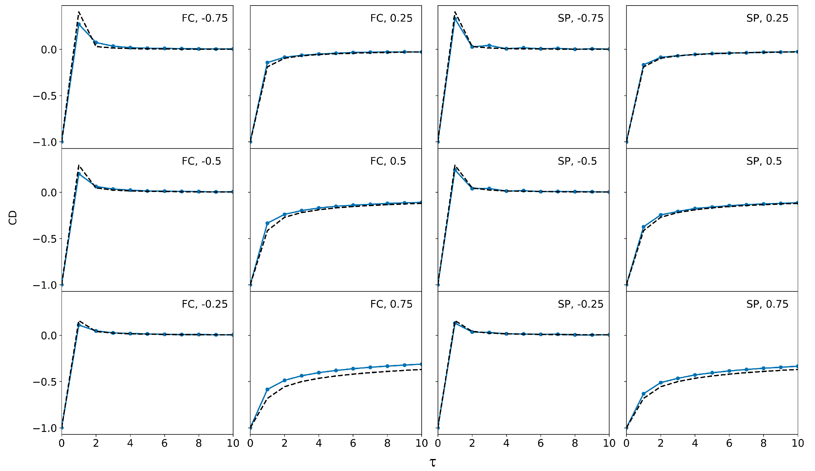
In order to validate the results obtained from the analysis of the codifference function, we compared the analytical form of $CD(1,-1;\tau )$ given by Equation (A9) for Gaussian coloured noises with the results of the numerical simulations for the same coloured noises and for $\beta \in [-0.75,0.75]$; in our simulations, we produced coloured noises by both fractional calculus and spectral processing (see Figure 4). The values obtained from numerical simulations match nicely with theoretical predictions. The characterization of the daughter processes demonstrates that second-order statistics, such as PSD and ACF, can detect the colour of a noise but cannot discriminate the PDF of the original mother noise. On the contrary, kurtosis and CD are effective tools to separate coloured noises generated from various white noise distributions. For all coloured noises produced from the original mother process, kurtosis can provide information regarding the PDF of the mother process; it will be greater than 3 for leptokurtic mother white noise and smaller than 3 for a platykurtic one. Furthermore, CD for lag-time zero effectively maintains the value, within a small fluctuating range, of the original mother process for all coloured noises that are derived from it, and consequently it can be used as a fingerprint for the detection of the PDF family (lepto-, platy- or meso-kurtic) it belongs to. The lag-time dependence of the co-difference function is interesting. No matter from which PDF of white noise a daughter process was derived, CD exhibits nearly the same time dependence when a colour value is within the expected range [0.25, 0.75] (see Figure 3). On the other hand, there is a definite distinction between the same colour derived from different white noise PDF’s when the colour value is within the range $[-0.75,-0.25]$. According to Figure 3, the uniform distribution-generated coloured noises have the absolute maximum in comparison to the other noises, followed by the coloured noises generated by the Gaussian distribution. Conversely, noise generated based on the Laplace distribution always has the lowest maxima. The properties under consideration do not appear to be impacted by whether coloured noise is produced using FC or SP. One can note the best placements of the power spectrum, but the latter has to do with how to produce a coloured noise, as already discussed in the text.

Four distinct white noise distributions were chosen, and the coloured noises produced by them have been analysed in the present work. These distributions find application in many different branches of the sciences; just to name a few: (i) any aspect of science for Gaussian white noise; (ii) resonance, spectroscopy, prices of speculative assets in economy, distribution of hypocenters on focal spheres of earthquakes in geophysics [25,45] for Cauchy; (iii) formation of images by the eyes [46] in decision making for systems by maximising the information for Uniform; and (iv) communications, economics, engineering, and finance for Laplace [29]. The present work can be extended in many different ways. First, the same initial white noise distributions can be chosen without the condition of SaS, and thus, apart from kurtosis and CD, the skewness can also be examined in order to see if this property for coloured noises also retains characteristics of the initial white noises. In addition, different white noises than those used in this work can be selected as seeds, and of interest will be if kurtosis and CD maintain some of the properties of the initial white noises in the way we found in this work. A detailed investigation of various white noise distributions can lead to a general conclusion about the behaviour of kurtosis and CD. A positive answer—common behaviour—will support studies where a coloured noise finding (non-equilibrium process) can directly indicate the form of equilibrium from which it came, thus indicating possible mechanisms acting on the equilibrium state.

5. Conclusions

In summary, we report the characterization of stationary coloured noises with spectral exponents ranging from $-0.75$ to 0.75 (i.e., fractional noises) generated from different types of white noises using appropriate operators acting either in the time domain (fractional calculus) or in the frequency domain (spectral processing). In particular, we chose four different probability distributions (Gaussian, Uniform, Laplace, and Cauchy) from which we sampled white noise vectors (mother processes). Two indices, kurtosis and codifference, perform well in discriminating the white noise distributions that stationary coloured noises originate from. Both of them actually preserve, to some extent, the properties of the original white noise distribution, in contrast to second-order statistics such as power spectral density and the autocorrelation function, which only return the main noise characteristics, power spectral exponent, and persistent or anti-persistent character. The value of kurtosis for the initial white noises depends on the existence or absence of outliers in excess with respect to Gaussian distribution. Its reference value is 3 for Gaussian white noise, goes up to 6 for Laplace white noise (leptokurtic), and reduces to 1.8 for Uniform white noise (platykurtic). Daughter processes have values of kurtosis close to those of the mother process for power spectrum exponents that are small in absolute value. As the exponent increases in absolute value, kurtosis decreases for coloured noises that come from Laplace white noise and increases for coloured noises created by uniform white noise. In all these cases, the values of kurtosis are above (for Laplace) or below (for Uniform) the reference value of 3. This behaviour states that daughter distributions have a lower (for Laplace) or higher (for Uniform) number of outliers with respect to their mother’s processes. The codifference function, for lag zero, provides a characteristic value for each white noise distribution, and this value is preserved for all coloured noises produced by it.

References

1. McClintock, P.V.E. Unsolved problems of noise. Nature 1999, 401, 23–25. [Google Scholar] [CrossRef] [Green Version]
2. Ceriotti, M.; Bussi, G.; Parrinello, M. Colored-Noise Thermostats à la Carte. J. Chem. Theor. Comput. 2010, 6, 1170. [Google Scholar] [CrossRef] [Green Version]
3. Yamamoto, E.; Akimoto, T.; Yesui, M.; Yasuoka, K. Origin of 1/f noise in hydration dynamics on lipid membrane surfaces. Sci. Rep. 2015, 5, 8876. [Google Scholar] [CrossRef] [Green Version]
4. Zhu, Z.; Sheng, N.; Fang, H.P.; Wan, R.Z. Colored spectrum characteristics of thermal noise on the molecular scale. Phys. Chem. Chem. Phys. 2016, 18, 30189. [Google Scholar] [CrossRef]
5. Lugli, F.; Zerbetto, F. Dynamic Self-Organization and Catalysis: Periodic versus Random Driving Forces. J. Phys. Chem. C 2019, 123, 825. [Google Scholar] [CrossRef]
6. Halley, J.M.; Kunin, E. Extinction risk and the 1/f family of noise models. Theor. Biol. 1999, 56, 215. [Google Scholar] [CrossRef] [PubMed]
7. Cuddington, K.M.; Yodzis, P. Black noise and population persistence. Philos. Trans. R. Soc. Lond. B Biol. Sci. 1999, 266, 969. [Google Scholar] [CrossRef]
8. Kasdin, N.J. Discrete Simulation of Colored Noise and Stochastic Processes and 1/fα Power Law Noise Generation. Proc. IEEE 1995, 83, 802–827. [Google Scholar] [CrossRef]
9. Greenhall, C.A. FFT-Based Methods for Simulating Flicker Fm. In Proceedings of the 34th Annual Precise Time and Time Interval Systems and Applications Meeting, Reston, VA, USA, 3–5 December 2002; pp. 481–491. [Google Scholar]
10. Fox, R.F.; Gatland, I.R.; Roy, R.; Vemuri, G. Fast, accurate algorithm for numerical simulation of exponentially correlated colored noise. Phys. Rev. A 1988, 38, 5938. [Google Scholar] [CrossRef] [Green Version]
11. Gillespie, D.T. Exact numerical simulation of the Ornstein-Uhlenbeck process and its integral. Phys. Rev. E 1996, 54, 2084. [Google Scholar] [CrossRef] [Green Version]
12. Miller, K.S.; Ross, B. An Introduction to Fractional Calculus and Fractional Differential Equations; Wiley: New York, NY, USA, 1993. [Google Scholar]
13. Kasdin, N.J.; Walter, D. Discrete simulation of power law noise. In Proceedings of the IEEE Frequency Control Symposium, Hershey, PA, USA, 27–29 May 1992; pp. 274–283. [Google Scholar]
14. Timmer, J.; Köning, M. On generating power law noise. Astron. Astrophys. 1995, 300, 707–710. [Google Scholar]
15. Di Matteo, T. Multi-scaling in finance. Quant. Financ. 2007, 1, 21–36. [Google Scholar] [CrossRef]
16. Krapf, D.; Lukat, N.; Marinari, E.; Metzler, R.; Oshanin, G.; Selhuber-Unkel, C.; Squarcini, A.; Stadler, L.; Weiss, M.; Xu, X. Spectral Content of a Single Non-Brownian Trajectory. Phys. Rev. X 2019, 9, 011019. [Google Scholar] [CrossRef] [Green Version]
17. Bakalis, E.; Ferraro, A.; Gavriil, V.; Pepe, F.; Kollia, Z.; Cefalas, A.C.; Malapelle, U.; Sarantopoulou, E.; Troncone, G.; Zerbetto, F. Universal Markers Unveil Metastatic Cancerous Cross-Sections at Nanoscale. Cancers 2022, 14, 3728. [Google Scholar] [CrossRef] [PubMed]
18. Bakalis, E.; Parent, L.R.; Vratsanos, M.; Park, C.; Gianneschi, N.C.; Zerbetto, F. Complex Nanoparticle Diffusional Motion in Liquid-Cell Transmission Electron Microscopy. J. Phys. Chem. C 2020, 124, 14881–14890. [Google Scholar] [CrossRef]
19. Bakalis, E.; Gavriil, V.; Cefalas, A.C.; Kollia, Z.; Zerbetto, F.; Sarantopoulou, E. Viscoelasticity and Noise Properties Reveal the Formation of Biomemory in Cells. J. Phys. Chem. B 2021, 125, 10883–10892. [Google Scholar] [CrossRef] [PubMed]
20. He, Y.; Burov, S.; Metzler, R.; Barkai, E. Random Time-Scale Invariant Diffusion and Transport Coefficients. Phys. Rev. Lett. 2008, 101, 058101. [Google Scholar] [CrossRef] [Green Version]
21. Burov, S.; Jeon, J.H.; Metzler, R.; Barkai, E. Single particle tracking in systems showing anomalous diffusion: The role of weak ergodicity breaking. Phys. Chem. Chem. Phys. 2011, 13, 1800–1812. [Google Scholar] [CrossRef] [Green Version]
22. Schwarzl, M.; Godec, A.; Metzler, R. Quantifying non-ergodicity of anomalous diffusion with higher order moments. Sci. Rep. 2017, 7, 378. [Google Scholar] [CrossRef] [Green Version]
23. Kokoszka, P.S.; Taqqu, M.S. Infinite variance stable ARMA processes. J. Time Ser. Anal. 1994, 15, 203–220. [Google Scholar] [CrossRef]
24. Fama, E.F.; Roll, R. Some properties of symmetric stable distributions. Am. Stat. Assoc. J. 1968, 63, 817–836. [Google Scholar]
25. Samorodnitsky, G.; Taqqu, M. Stable Non-Gaussian Random Processes: Stochastic Models with Infinte Variance, 1st ed.; Chapman and Hall: London, UK, 1994. [Google Scholar]
26. Laue, G. Remarks on the relation between fractional moments and fractional derivatives of characteristic functions. J. Appl. Probab. 1980, 17, 456–466. [Google Scholar] [CrossRef]
27. Matsui, M.; Pawlas, Z. Fractional absolute moments of heavy tailed distributions. Braz. J. Probab. Stat. 2016, 30, 272–298. [Google Scholar] [CrossRef]
28. Kozubowski, T.J.; Rachev, S.T. The theory of Geometric Stable Distributions and its use in modeling financial data. Eur. J. Oper. Res. 1994, 74, 310–324. [Google Scholar] [CrossRef]
29. Kotz, S.; Kozubowski, T.J.; Podgórski, K. The Laplace Distribution and Generalizations: A Revisit with Applications to Communications, Economics, Engineering, and Finance; Birkhäuser: Boston, MA, USA, 2001. [Google Scholar]
30. MATLAB and Statistics Toolbox, Release 2012b; The MathWorks, Inc.: Natick, MA, USA, 2012.
31. Box, G.E.P.; Muller, M.E. A Note on the Generation of Random Normal Deviates. Ann. Math. Stat. 1958, 29, 610. [Google Scholar] [CrossRef]
32. Lee, D.U.; Villasenor, J.D.; Luk, W.; Leong, P.H.W. A Hardware Gaussian Noise Generator Using the Box-Muller Method and Its Error Analysis. IEEE Trans. Comput. 2006, 55, 659. [Google Scholar] [CrossRef] [Green Version]
33. Eltoft, T.; Taesu, K.; Te-Won, L. On the multivariate Laplace distribution. IEEE Signal Process. Lett. 2006, 13, 300. [Google Scholar] [CrossRef]
34. Johnson, N.L.; Kotz, S.; Balakrishnan, N. Continuous Univariate Distributions, 2nd ed.; Wiley: New York, NY, USA, 1994; Volume 1. [Google Scholar]
35. Beck, C.; Cohen, E.G.D. Superstatistics. Physica A 2003, 322, 267–275. [Google Scholar] [CrossRef] [Green Version]
36. Poldubny, I. Fractional Differential Equations; Academic Press: Cambridge, MA, USA, 1999. [Google Scholar]
37. Regadio, A.; Tabero, J.; Sanchez-Prieto, S. A Method for Colored Noise Generation. Nucl. Instrum. Methods Phys. Res. A 2016, 811, 25. [Google Scholar] [CrossRef]
38. West, B.; Bologna, M.; Grigolini, P. Physics of Fractal Operator; Springer: New York, NY, USA, 2003. [Google Scholar]
39. West, B.J. Colloquium: Fractional calculus view of complexity: A tutorial. Rev. Mod. Phys. 2014, 86, 1169. [Google Scholar] [CrossRef]
40. Scherer, R.; Kalla, S.L.; Tang, Y.; Huang, J. The Grünwald–Letnikov method for fractional differential equations. Comput. Math. Appl. 2011, 62, 902. [Google Scholar] [CrossRef] [Green Version]
41. Gorenflo, R.; Mainardi, F. Fractional Calculus; Springer: Vienna, Austria, 1997. [Google Scholar]
42. de Oliveira, E.C.; Tenreiro Machado, J.A. A Review of Definitions for Fractional Derivatives and Integral. Math. Probl. Eng. 2014, 2014, 238459. [Google Scholar] [CrossRef] [Green Version]
43. Zhivomirov, H. A Method for Colored Noise Generation. J. Acoust. Vibr. 2018, 15, 14. [Google Scholar]
44. Fougere, P.F. On the Accuracy of Spectrum Analysis of Red Noise Processes Using Maximum Entropy and Periodogram Methods: Simulation Studies and Application to Geophysical Data. J. Geophys. Res. 1985, 90, 4355. [Google Scholar] [CrossRef]
45. Moss, F.; McClintock, P.V.E. Noise in Nonlinear Dynamical Systems: Theory of Noise Induced Processes in Special Applications; Cambridge University Press: Cambridge, UK, 1989; Volume 2. [Google Scholar]
46. Bakalis, E.; Fujie, H.; Zerbetto, F.; Tanaka, Y. Multifractal structure of microscopic eye–head coordination. Physica A 2018, 512, 945–953. [Google Scholar] [CrossRef]
47. Beran, J. Statistics for Long-Memory Processes; Chapman and Hall: New York, NY, USA, 1994. [Google Scholar]
48. Rosadi, D. Testing for independence in heavy-tailed time series using the codifference function. Comput. Stat. Data Anal. 2009, 53, 4516–4529. [Google Scholar] [CrossRef]
49. Eke, A.; Herman, P.; Bassingthwaighte, J.B.; Raymond, G.M.; Percival, D.B.; Cannon, M.; Balla, I.; Ikrenyi, C. Physiological time series: Distinguishing fractal noises from motions. Pflüg. Arch. Eur. J. Physiol. 2000, 439, 403. [Google Scholar] [CrossRef]
50. Wyłomańska, A.; Chechkin, A.; Gajda, J.; Sokolov, I.M. Codifference as a practical tool to measure interdependence. Physica A 2015, 421, 412–429. [Google Scholar] [CrossRef] [Green Version]
Figure 1. White Noises: Trajectories (first column), probability distribution (second column), kurtosis (third column), and codifference function (fourth column) are displayed for Gaussian (blue), uniform (green), Laplace (orange), and Cauchy (yellow) PDFs.
Fractalfract 07 00600 g001
Figure 2. Autocorrelation (ACF) and Power Spectral Density (PSD) for all produced coloured noises. The inset defines the operator used for the creation of noise sequence and the β value of the fractional noise: blue for daughter noises coming from Gaussian white noise, green for daughter noises coming from Uniform white noise, orange for those coming from Laplace white noise, and yellow for those coming from Cauchy white noise.
Fractalfract 07 00600 g002
Figure 3. Kurtosis and codifference functions for all produced coloured noises. The inset defines the PDF of the mother process and the operator used for the creation of a noise sequence.
Fractalfract 07 00600 g003
Figure 4. Codifference function as a function of the lag time as predicted by simulations and by Equation (A9).
Fractalfract 07 00600 g004