Influences of the Order of Derivative on the Dynamical Behavior of Fractional-Order Antisymmetric Lotka–Volterra Systems

Abstract

This paper studies the dynamic behavior of a class of fractional-order antisymmetric Lotka–Volterra systems. The influences of the order of derivative on the boundedness and stability are characterized by analyzing the first-order and $0<\alpha <1$-order antisymmetric Lotka–Volterra systems separately. We show that the order does not affect the boundedness but affects the stability. All solutions of the first-order system are periodic, while the $0<\alpha <1$-order system has no non-trivial periodic solution. Furthermore, the $0<\alpha <1$-order system can be reduced on a two-dimensional space and the reduced system is asymptotically stable, regardless of how close to zero the order of the derivative used is. Some numerical simulations are presented to better verify the theoretical analysis.

1. Introduction

The classical Lotka–Volterra equations (LVE for short) can be expressed in a compact form as

$$\frac{\mathrm{d}{x}_i\left(t\right)}{\mathrm{d}t}=x_i{\left(Ax\right)}_i,i=1,2,\cdots ,n,$$

where $A={\left(a_{ij}\right)}_{n\times n}$ is a real matrix, $x={(x_1,x_2,\cdots ,x_n)}^{\mathrm{T}}\in {\mathbb{R}}^n$. It was first introduced by Volterra [1] in the context of predator–prey oscillations in population biology. Under the background of the predator–prey relationship, LVE is used to study the dynamic change of an individual population. The different species are labeled by i (or j) with $i,j=1,2,\cdots ,n$, $x_i\left(t\right)$ represents the density of population of species i at the time of t, and the parameter $a_{ij}$ represents the impact of species j on species i: $a_{ij}>0$ indicates that species i preys on species j, $a_{ij}<0$ indicates that species i is the prey of j, and $a_{ij}=0$ means that species i and j have no predation relationship. The size of $a_{ij}$ is seen as the predatory efficiency. Nowadays it is also of central importance to many other fields of science (e.g., plasma physics and chemical kinetics [2]). Mathematically speaking, many important results on the Lotka–Volterra system have been produced, such as global asymptotic behavior and bifurcation [3,4,5]. In particular, the three-dimensional antisymmetric LVE is known as the replicator equation of the rock–paper–scissors game [6]. Furthermore, the rock–paper–scissors dynamical system is found to be rather common for biological systems, for example, polymorphic groups of side-blotched lizards [7], microbial laboratory communities [8].

In recent years, fractional calculus has attracted much attention from researchers [9,10,11,12,13,14]. The fractional derivative at time t is not defined locally and depends on the total effects of the classical integer-order derivatives on the interval $[0,t]$, so it can be used to describe the variation of a system in which the instantaneous change rate depends on the past state, which is called the memory effect in a visualized manner [15,16,17]. We refer to [18,19,20,21,22,23] for some interpretations of physical and biological significance of fractional operators by supplying specific examples. Nowadays, many dynamical systems with integer order have been extended to the fractional-order systems. This extension allows us to explore and obtain some new behaviors. From the mathematical viewpoint, many researchers consider the influence of fractional derivatives on dynamic behavior [24,25,26]. In [27,28], the authors discuss that the chaos in integer-order systems disappears in their fractional-order counterparts with sufficiently small values of fractional order. In [29], the authors extend the classical model of the prey–predator model to a new model based on the Caputo fractional derivatives and propose that the new model is very sensitive to varying the fractional order. Reference [30] considers a three-dimensional fractional-order slow–fast prey–predator model and reveals that the fractional-order exponent has an impact on the stability and the existence of Hopf bifurcations in this model.

In this paper, we consider a fractional-order antisymmetric Lotka–Volterra system composed of three species

$${}_0{D}_t^{\alpha }{x}_i\left(t\right)=x_i{\left(Ax\right)}_i,i=1,2,3,$$

(1)

with the initial value

$$x\left(0\right)=b,$$

(2)

where ${}_0{D}_t^{\alpha }$ is the Caputo fractional derivative with $\alpha \in (0,1]$, $A={\left(a_{ij}\right)}_{3\times 3}$ is an antisymmetric matrix ($a_{ij}=-a_{ji}$), $x={(x_1,x_2,x_3)}^{\mathrm{T}}$ and $b={(b_1,b_2,b_3)}^{\mathrm{T}}$. Considering the practical significance, we always assume that $b_i>0$, $i=1,2,3$. We assume that three species dominate each other according to the popular rock–paper–scissors game rules, as illustrated in Figure 1; that is, $a_{12},a_{23},a_{31}>0$, which means that each predator has an effective predation probability.

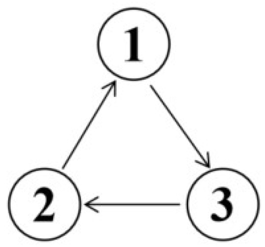
Figure 1. Illustration of the predation interaction rules among species in the rock–paper–scissors model. Arrows from j to i indicate $a_{ij}>0$, i.e., species i preys on species j in a predator–prey relationship.

The model is an extension of the classical antisymmetric Lotka–Volterra model to a fractional order, but there are essential differences between $\alpha =1$ and $0<\alpha <1$ on the dynamical behavior. Our aim is to characterize the influences of the order of derivative on antisymmetric Lotka–Volterra systems (1).

We first prove that for any $\alpha \in (0,1]$, ${\sum }_{i=1}^3{x}_i\left(t\right)$ is a conserved quantity, and all $x_i$ stays away from zero for all times. Note that in the context of population dynamics, this means that the total number of individuals for all species is conserved and all species coexist independently of the predatory efficiency. We further analyze the influences of the order of derivative on the stability of the system (1). The results show that all solutions of the first-order system are periodic, while the $0<\alpha <1$-order system has no non-trivial periodic solution. Furthermore, for any choice of $a_{12},a_{23},a_{31}>0$, all solutions of the $0<\alpha <1$-order system starting near equilibrium points go towards a unique equilibrium point on the plane depending on ${\sum }_{i=1}^3{b}_i$, regardless of how close to zero the order of the derivative used is. This means that in this model if the equilibrium state is slightly disturbed, as long as the total number of species remains unchanged, it will always return to the original equilibrium state after a long time. This may reflect the memory of the fractional-order system. Finally, we give some numerical simulations.

The paper is organized as follows. In Section 2, some basic concepts and preliminary results are presented. In Section 3, the conclusions of the boundedness of solutions are given. In Section 4, the influences of the order of derivative on stability are characterized. Some numerical simulations are provided in Section 5. Section 6 gives the conclusions.

2. Preliminaries

This section includes some basic preliminaries. We review some definitions and preliminary results that will be required for our theorems.

Definition 1

([16]). The Riemann–Liouville fractional integral ${}_{0}I_t^{\alpha }f$ of order $\alpha >0$ is defined by

$$\left({}_{0}I_t^{\alpha }f\right)\left(t\right):=\frac{1}{\mathsf{\Gamma }\left(\alpha \right)}{\int }_0^t{(t-s)}^{\alpha -1}f\left(s\right)ds,t>0,$$

where $\mathsf{\Gamma }\left(\alpha \right)$ is the Gamma function.

The Riemann–Liouville fractional derivative ${}_0{}^{\mathit{RL}}D_t^{\alpha }y$ of order $\alpha >0$ is defined by

$$\left({}_0^{RL}{D}_t^{\alpha }y\right)\left(t\right):={\left(\frac{\mathrm{d}}{\mathrm{d}t}\right)}^n\left({}_0{I}_t^{n-\alpha }y\right)\left(t\right),n=\left[\alpha \right]+1,$$

where $\left[\alpha \right]$ means the integer part of α.

Definition 2

([16]). The Caputo fractional derivative ${}_0{D}_t^{\alpha }y$ of order $\alpha >0$ is defined by

$$\left({}_0{D}_t^{\alpha }y\right)\left(t\right):=\left({}_0^{RL}{D}_s^{\alpha }\left[y\left(s\right)-\sum _{k=0}^{n-1}\frac{y^{\left(k\right)}\left(0\right)}{k!}{s}^k\right]\right)\left(t\right),$$

where

$$n=\left[\alpha \right]+1\mathrm{for}\alpha \notin {\mathbb{N}}_0;n=\alpha \mathrm{for}\alpha \in {\mathbb{N}}_0.$$

Lemma 1

([16]). Let $0\le \alpha \le 1$. If $y\left(t\right)$ is an absolutely continuous function on $[0,c]$$(c\in \mathbb{R}+)$, then the Caputo fractional derivative $\left({}_0{D}_t^{\alpha }y\right)\left(t\right)$ exists almost everywhere on $[0,c]$.

(a)

If $0<\alpha <1$, $\left({}_0{D}_t^{\alpha }y\right)\left(t\right)$ is represented by

$$\left({}_0{D}_t^{\alpha }y\right)\left(t\right)=\frac{1}{\mathsf{\Gamma }(1-\alpha )}{\int }_0^t\frac{y^{\prime }\left(t\right)}{{(t-s)}^{\alpha }}\mathrm{d}s.$$

(b)

If $\alpha =1$, $\left({}_0{D}_t^{\alpha }y\right)\left(t\right)=y^{\prime }\left(t\right)$.

Definition 3

([16]). The Mittag–Leffler function is defined as

$$E_{\alpha }\left(z\right)=\sum _{k=0}^{\infty }\frac{z^k}{\mathsf{\Gamma }(\alpha k+1)},\alpha >0,z\in \mathbb{C}.$$

Lemma 2

([16]). The solution to the problem

$${}_0{D}_t^{\alpha }u\left(t\right)-\lambda u\left(t\right)=0,u\left(0\right)=c$$

with $0<\alpha <1$ and $\lambda ,c\in \mathbb{R}$ has the form

$$u\left(t\right)=c{E}_{\alpha }\left(\lambda t^{\alpha }\right).$$

Lemma 3.

Assume that $0<\alpha <1$ and $f:[0,+\infty )\to {\mathbb{R}}^{+}$ is continuously differentiable. Then

$${}_0{D}_t^{\alpha }lnf\left(t\right)\ge \frac{{}_0{D}_t^{\alpha }f\left(t\right)}{f\left(t\right)},t>0.$$

Proof. 

According to Definition 2, we only need to show that

$${}_0{D}_t^{\alpha }f\left(t\right)-f\left(t\right){}_0{D}_t^{\alpha }lnf\left(t\right)={\int }_0^t{(t-s)}^{-\alpha }\left[f^{\prime }\left(s\right)-\frac{f\left(t\right)f^{\prime }\left(s\right)}{f\left(s\right)}\right]\mathrm{d}s\le 0,t>0.$$

(3)

By the integration-by-part formula, we conclude that

$$\begin{array}{cc}\hfill & {\int }_0^t{(t-s)}^{-\alpha }\left[f^{\prime }\left(s\right)-\frac{f\left(t\right)f^{\prime }\left(s\right)}{f\left(s\right)}\right]\mathrm{d}s\hfill \\ =\hfill & {\int }_0^t{(t-s)}^{-\alpha }\frac{\mathrm{d}}{\mathrm{d}s}\left[f\left(s\right)-f\left(t\right)-f\left(t\right)ln\frac{f\left(s\right)}{f\left(t\right)}\right]\mathrm{d}s\hfill \\ =\hfill & \underset{s\to t}{lim}\frac{f\left(s\right)-f\left(t\right)-f\left(t\right)ln\frac{f\left(s\right)}{f\left(t\right)}}{{(t-s)}^{\alpha }}-t^{-\alpha }\left(f\left(0\right)-f\left(t\right)-f\left(t\right)ln\frac{f\left(0\right)}{f\left(t\right)}\right)\hfill \\ \hfill & -\alpha {\int }_0^t\left(f\left(s\right)-f\left(t\right)-f\left(t\right)ln\frac{f\left(s\right)}{f\left(t\right)}\right){(t-s)}^{-\alpha -1}\mathrm{d}s.\hfill \end{array}$$

(4)

First, by L’Hôpital’s rule, we can obtain the first term on the right side of Equation (4) equal to

$$\underset{s\to t}{lim}\frac{f^{\prime }\left(s\right)-f\left(t\right)\frac{f^{\prime }\left(s\right)}{f\left(s\right)}}{\alpha {(t-s)}^{\alpha -1}}=0.$$

(5)

Next, we estimate the other two items. It is understood that

$$\xi -ln\xi -1\ge 0,\forall \xi \in {\mathbb{R}}^{+}.$$

Then, for any fixed t and $\tau$, we have

$$f\left(\tau \right)-f\left(t\right)-f\left(t\right)ln\frac{f\left(\tau \right)}{f\left(t\right)}\ge 0.$$

Therefore, we have that the second term on the right side of Equation (4) is non-positive when $\tau =0$. For any $s\in (0,t)$, $f\left(s\right)-f\left(t\right)-f\left(t\right)ln\frac{f\left(s\right)}{f\left(t\right)}\ge 0$, which shows that the last integral item of Equation (4) is non-positive. Therefore, (4) is non-positive; that is, (3) holds. □

Lemma 4

(Fractional Comparison Principle [16]). Let ${}_0{D}_t^{\alpha }x\left(t\right)\le {}_0{D}_t^{\alpha }y\left(t\right)$ and $x\left(0\right)=y\left(0\right)$, where $0<\alpha <1$. Then $x\left(t\right)\le y\left(t\right)$.

Lemma 5.

Let $L\left(x\right)$ be a differentiable function defined on an open set U containing $x^{*}$ in ${\mathbb{R}}^n$. Suppose that $L\left(x^{*}\right)=0$ and $L\left(x\right)>0$ if $x\ne x^{*}$. Then, if $c>0$ is small enough, each connected component of $L\left(x\right)=c$ is a closed surface surrounding $x^{*}$.

Proof. 

Let $\delta >0$ be small enough that a closed ball centering at $x^{*}$ of radius $\delta$ lies entirely in U, that is,

$$B_{\delta }\left(x^{*}\right)=\{x\in {\mathbb{R}}^n|\parallel x-x^{*}\parallel \le \delta \}\subset U.$$

The boundary of $B_{\delta }\left(x^{*}\right)$ is the sphere $S_{\delta }\left(x^{*}\right)$ of radius $\delta$ and center $x^{*}$, i.e.,

$$S_{\delta }\left(x^{*}\right):=\{x\in B_{\delta }\left(x^{*}\right)|\parallel x-x^{*}\parallel =\delta \}.$$

By the compactness of $S_{\delta }\left(x^{*}\right)$ and the continuity of L, there is a minimum $x_{*}\in S_{\delta }^{*}$ of L restricted on the sphere. Let $\gamma$ be the minimum value of L on the sphere $S_{\delta }^{*}$, i.e.,

$$\gamma =\underset{x\in S_{\delta }\left(x^{*}\right)}{min}L\left(x\right)=L\left(x_{*}\right).$$

For any $0<c<\gamma$, let

$$W_c=\{x\in U|L\left(x\right)=c\}\subseteq B_{\delta }\left(x^{*}\right).$$

For any continuous curve $\xi \subseteq B_{\delta }\left(x^{*}\right)$ connecting $x^{*}$ and any point on $S_{\delta }\left(x^{*}\right)$, there exists at least one point $z\in \xi$ satisfying $L\left(\xi \right)=c$ by the intermediate value theorem of the continuous function ${L|}_{\xi }$ and $L\left(x^{*}\right)=0$. Then no curve starting from $x^{*}$ to $S_{\delta }\left(x^{*}\right)$ meets the set $W_c$. Hence, each connected component of $W_c$ is a closed surface. This proves that $W_c$ is a closed surface or a family of closed surfaces surrounding $x^{*}$. □

Lemma 6

([31]). Let $n>0$, $r>0$, $\phi \in [-\pi ,\pi ]$ and $\lambda =rexp\left(\mathrm{i}\phi \right)$. Denote $y\left(t\right):=E_n\left(-\lambda t^n\right)$. Then,

(a)

$\underset{x\to \infty }{lim}y\left(t\right)=0$ if $\left|\phi \right|<n\pi /2$,

(b)

$y\left(t\right)$ is unbounded as $x\to \infty$ if $\left|\phi \right|>n\pi /2$.

Let $0<\alpha <1$. The homogeneous linear system is given by

$${}_0{D}_t^{\alpha }x\left(t\right)=Bx\left(t\right),x\left(t\right)\in {\mathbb{R}}^n$$

(6)

with $x\left(0\right)=b$, where B is an $n\times n$ real matrix. The nonlinear system is given by

$${}_0{D}_t^{\alpha }x\left(t\right)=f\left(x\left(t\right)\right),x\left(t\right)\in {\mathbb{R}}^n$$

(7)

with $x\left(0\right)=b$, where $f\left(x\right)$ is continuous.

Definition 4

([32]). The system (6) is said to be asymptotically stable if $\underset{t\to +\infty }{lim}\parallel x\left(t\right)\parallel =0$.

Definition 5

([32]). The point e is an equilibrium point of system (7) if and only if $f\left(e\right)=0$.

Definition 6

([32]). Suppose that e is an equilibrium point of system (7) and $Df\left(e\right)$ is linearized matrix of f at e. If all the eigenvalues λ of $Df\left(e\right)$ satisfy $\left|\lambda \right|\ne 0$ and $|arg\left(\lambda \right)|\ne \frac{\pi \alpha }{2}$, then we call e a hyperbolic equilibrium point.

Lemma 7

([32]). If e is a hyperbolic equilibrium point of (7), then vector field $f\left(x\right)$ is topologically equivalent with its linearization vector field $Df\left(e\right)x$ in the neighborhood of e.

3. Boundedness Results

In this section, we will find the significantly common property between the first-order and the $0<1<\alpha$-order system (1). The boundedness is independent of the order of derivative. For any choice of $a_{12},a_{23},a_{31}>0$, all solutions of the systems are bounded for all time, and the lower bound is away from zero for each solution.

Lemma 8.

For arbitrary solutions $x={(x_1,x_2,x_3)}^{\mathrm{T}}$ of system (1) with initial value (2), $H\left(x\right):={\displaystyle \sum _{i=1}^3}{x}_i$ is a conserved quantity.

Proof. 

From the antisymmetry of A, it can be obtained that x satisfies

$${}_0{D}_t^{\alpha }\left(\sum _{i=1}^3{x}_i\left(t\right)\right)=\sum _{i=1}^3{}_0{D}_t^{\alpha }{x}_i\left(t\right)=\sum _{i=1}^3{x}_i{\left(Ax\right)}_i=0,\forall t>0.$$

(8)

If $0<\alpha <1$, from Lemma 2, we have

$$\sum _{i=1}^3{x}_i\left(t\right)=\sum _{i=1}^3{x}_i\left(0\right)\mathrm{for}t>0.$$

(9)

If $\alpha =1$, it is clear that (8) implies (9). The proof is complete. □

We next show that $x_i\left(t\right)$ remains bounded away from 0. By calculating the $Ar=0$, we can obtain the kernel of A is

$$ker\left(A\right)=\{r\in {\mathbb{R}}^3|r=s{(a_{23},a_{31},a_{12})}^{\mathrm{T}},s\in \mathbb{R}\}.$$

By assumption $a_{12},a_{23},a_{31}>0$, we have $ker\left(A\right)\ne \varnothing$. On the domain ${\mathbb{R}}_{+}^3$, we define a function

$$V\left(z\right)=\sum _{i=1}^3\left(z_i-y_i-y_{i}ln\frac{z_i}{y_i}\right)$$

(10)

for one fixed $y\in ker\left(A\right)$ with $y={(y_1,y_2,y_3)}^{\mathrm{T}}>0$.

Lemma 9.

For any solution $x\left(t\right)={(x_1\left(t\right),x_2\left(t\right),x_3\left(t\right))}^{\mathrm{T}}$ of the system (1) with initial value (2), $V\left(x\right)$ has the following properties along $x\left(t\right)$.

(i)

If $\alpha =1$, $V\left(x\right(t\left)\right)\equiv V\left(b\right)$ for all $t>0$.

(ii)

If $0<\alpha <1$, $V\left(x\right(t\left)\right)\le V\left(b\right)$ for all $t>0$.

Proof. 

For case (i), considering the time derivative of $V\left(x\right(t\left)\right)$ and employing Equation (1) yields

$$\begin{array}{cc}\hfill & \frac{\mathrm{d}}{\mathrm{d}t}\left(\sum _{i=1}^3\left(x_i\left(t\right)-y_i-y_{i}ln\frac{x_i\left(t\right)}{y_i}\right)\right)\hfill \\ =\hfill & \frac{\mathrm{d}}{\mathrm{d}t}\left(\sum _{i=1}^3{x}_i\left(t\right)\right)-\sum _{i=1}^3\left(\frac{y_i}{x_i\left(t\right)}\frac{\mathrm{d}{x}_i\left(t\right)}{\mathrm{d}t}\right)\hfill \\ =\hfill & \frac{\mathrm{d}}{\mathrm{d}t}\left(\sum _{i=1}^3{x}_i\left(t\right)\right)-\sum _{i=1}^3{y}_i{\left(Ax\left(t\right)\right)}_i.\hfill \end{array}$$

(11)

From Lemma 8, $\frac{\mathrm{d}}{\mathrm{d}t}{\displaystyle \sum _{i=1}^3}{x}_i\left(t\right)=0$. According to the antisymmetry of A and $y\in ker\left(A\right)$, we have

$$-\sum _{i=1}^3{y}_i{\left(Ax\right)}_i=\sum _{i=1}^3{x}_i{\left(Ay\right)}_i=0,\forall x\in {\mathbb{R}}_{+}^3.$$

Then (11) implies $\frac{\mathrm{d}}{\mathrm{d}t}V\left(x\left(t\right)\right)=0$. Therefore, case (i) holds.

For case (ii), we consider the Caputo fractional derivative of $V\left(x\right(t\left)\right)$. By (8) and Lemma 3, we deduce that

$$\begin{array}{cc}{}_0{D}_t^{\alpha }V\left(x\left(t\right)\right)=\hfill & {}_0{D}_t^{\alpha }\left(\sum _{i=1}^3{x}_i\right)-{}_0{D}_t^{\alpha }\left(\sum _i{y}_{i}ln{x}_i\right)\hfill \\ \hfill =& -\sum _i{y}_i{}_0{D}_t^{\alpha }\left(ln{x}_i\left(t\right)\right)\hfill \\ \hfill \le & -\sum _i{y}_i\frac{{}_0{D}_t^{\alpha }\left(x_i\left(t\right)\right)}{x_i\left(t\right)}\hfill \\ \hfill =& -\sum _{i=1}^3{y}_i{\left(Ax\right)}_i.\hfill \end{array}$$

(12)

Then, using the antisymmetry of A and definition of y, we have

$$-\sum _{i=1}^3{y}_i{\left(Ax\right)}_i=\sum _{i=1}^3{x}_i{\left(Ay\right)}_i=0.$$

Therefore, (12) leads to

$${}_0{D}_t^{\alpha }V\left(x\left(t\right)\right)\le 0,\forall t>0.$$

(13)

Let $y\left(t\right)\equiv V\left(x\right(0\left)\right)$, $\forall t>0$. Then, by Definition 2, we have ${}_0{D}_t^{\alpha }y\left(t\right)=0$. Therefore, combining (13) with the Fractional Comparison Principle (Lemma 4), we can obtain

$$V\left(x\right(t\left)\right)\le V\left(x\right(0\left)\right)\mathrm{for}\mathrm{all}t>0.$$

(14)

Case (ii) is complete. □

Corollary 1.

For $0<\alpha <1$, for any solution $x\left(t\right)={(x_1\left(t\right),x_2\left(t\right),x_3\left(t\right))}^{\mathrm{T}}$ of the system (1) with initial value (2), if $b\notin ker\left(A\right)$, then $V\left(x\right(t\left)\right)<V\left(b\right)$ for all $t>0$.

Proof. 

For $x\left(0\right)=b\notin ker\left(A\right)$, we can obtain $x\left(t\right)\not\equiv x\left(0\right)$. Then, by the proof of Lemma 3, we have $D_t^{\alpha }\left(\ln x_i\left(t\right)\right)\ne \frac{D_t^{\alpha }\left(x_i\left(t\right)\right)}{x_i\left(t\right)}$. Therefore, combining (12), we can derive from (13) that ${}_0{D}_t^{\alpha }V\left(x\left(t\right)\right)<0$ for $t>0$, which implies $V\left(x\right(t\left)\right)<V\left(x\right(0\left)\right)$ for all $t>0$. □

Theorem 1.

For arbitrary solutions $x={(x_1,x_2,x_3)}^{\mathrm{T}}$ of the system (1) with initial value (2), there exist constants $\delta ,\eta >0$ such that

$$\delta \le x_i\left(t\right)\le \eta ,\forall t>0,i=1,2,3.$$

(15)

Proof. 

By Lemma 8, the existence of $\eta$ is clear. Next, we will show the existence of $\delta$.

On the contrary, if there is no $\delta >0$ such that $\delta \le x_i\left(t\right)$ for all $t>0$ and $i=1,2,3,$ then there exists sequence $\left\{t_n\right\}$ with $t_n\to \infty$ as $n\to \infty$ satifying

$$\underset{n\to \infty }{lim}{x}_i\left(t_n\right)=0\mathrm{for}\mathrm{some}i\in \{1,2,3\}.$$

Then, $\underset{n\to \infty }{lim}ln{x}_i\left(t_n\right)=-\infty$ and $\underset{n\to \infty }{lim}V\left(x\left(t_n\right)\right)=+\infty$ by (10). This is contradictory with $V\left(x\right(t\left)\right)\le V\left(b\right)=const.$ by Lemma 9. Therefore, the assumption is false; that is, there exists $\delta >0$ satisfying (15). The proof is complete. □

4. Stability Results

In this section, we will characterize the effects of order $\alpha$ on the stability of the systems (1) by analyzing the long-time dynamical behaviors of first-order and $0<\alpha <1$-order systems, respectively.

We will use the conserved quantity $H\left(x\right)$, defined in Lemma 8, to reduce the system (1), so that the dynamics of the original system can be limited to the two-dimensional space. For any constant $c>0$, denote an open and bounded plane in ${\mathbb{R}}_{+}^3$ as

$$S_c:=\left\{v\in {\mathbb{R}}_{+}^3|v={(v_1,v_2,v_3)}^{\mathrm{T}},\sum _{i=1}^3{v}_i=c\right\}.$$

By Lemma 8, the solution to the system (1) with initial value $b=(b_1,b_2,b_3)\in {\mathbb{R}}_{+}^3$ contained in the plane $S_{H\left(b\right)}$. For convenience, we reduce the system (1) on the plane $S_1$. Consider the reduced system

$$\left\{\begin{array}{c}{}_0{D}_t^{\alpha }{x}_1=(a_{12}{x}_2+a_{13}(1-x_1-x_2))x_1:=f_1(x_1,x_2)\hfill \\ {}_0{D}_t^{\alpha }{x}_2=(-a_{12}{x}_1+a_{23}(1-x_1-x_2))x_2:=f_2(x_1,x_2)\hfill \end{array}\right.$$

(16)

on the domain $Z=\{x\in {\mathbb{R}}_{+}^2|x={(x_1,x_2)}^{\mathrm{T}},x_1+x_2<1\}$.

Lemma 10.

If $\alpha =1$, the system (16) has a unique equilibrium point, and all the solution curves are closed and around the equilibrium point on Z.

Proof. 

By assumption $a_{12},a_{23},a_{31}>0$, the two-dimensional system (16) has a unique equilibrium point

$$p=(p_1,p_2)=\left(\frac{a_{23}}{a_{23}+a_{31}+a_{12}},\frac{a_{31}}{a_{23}+a_{31}+a_{12}}\right).$$

Note that the function V restricted on the plane S can be rewritten as

$$\tilde{V}\left(w\right):=-p_{1}ln\frac{w_1}{p_1}-p_{2}ln\frac{w_2}{p_2}-(1-p_1-p_2)ln\frac{1-w_1-w_2}{1-p_1-p_2}.$$

In addition, $\tilde{V}$ is differentiable on domain Z. By simple calculation, we can find that $\tilde{V}$ satisfies

(a)

$\tilde{V}\left(z\right)>0$ if $z\in Z\backslash \left\{p\right\}$ and $\tilde{V}\left(p\right)=0,$

(b)

$\tilde{V}\left(z\right)\to +\infty$ as z goes to the boundary of domain $Z.$

For any $x_0\in Z$, there is a unique solution $x\left(t\right)=(x_1\left(t\right),x_2\left(t\right))$ to the system (16) with $x\left(0\right)=x_0$ in domain Z. First, we claim that the level set

$$W_{x_0}=\{x\in Z|\tilde{V}\left(x\right)=\tilde{V}\left(x_0\right)\}$$

is actually the orbit $x\left(t\right)$ and prove it with two steps.

Step 1. By Theorem 1, there are $0<\delta <\eta <1$ such that $\delta <x_1\left(t\right),x_2\left(t\right)<\eta$ for all $t>0$. We define a domain

$$Z_{\delta ,\eta }=\left\{x=(x_1,x_2)\in Z|\delta <x_1,x_2<\eta ,x_1+x_2<max\{1-\delta ,\eta \}\right\}.$$

Take the minimum value ${\gamma }_{\delta ,\eta }$ of $\tilde{V}$ on the boundary of domain $Z_{\delta ,\eta }$. According to property (b), we can choose $\delta >0$ sufficiently small and $\eta <1$ sufficiently close to 1 such that ${\gamma }_{\delta ,\eta }>\tilde{V}\left(x_0\right)$. Then $W_{x_0}$ is a family of closed curves around p by Lemma 5.

Step 2. Connect the origin and p with the segment $\xi \left(t\right)=t(p_1,p_2),t\in [0,1]$. For any $t\in (0,1]$, by direct calculation, we obtain

$$\frac{\mathrm{d}}{\mathrm{d}t}\tilde{V}\left(\xi \left(t\right)\right)<0.$$

This means that the function $\tilde{V}$ is monotonic along the segment $\xi$ from p to the origin. Hence, segment $\xi$ meets the set $W_{x_0}$ only one time. In conclusion, $W_{x_0}$ is one closed curve; that is, the solution curve starting from $x_0$ is a closed curve. The claim is proved.

By the arbitrariness of the initial value $x_0\in Z$, all the solution curves of the system (16) are closed curves around the equilibrium point. The proof is complete. □

In the following, we describe the entire behavior of the first-order antisymmetric Lotka–Volterra system (1).

Theorem 2.

If $\alpha =1$, all solutions of the systems (1) are periodic. Moreover, any solution curve is around the unique equilibrium point on one plane parallel with $S_1$.

Proof. 

For any initial value $b\in {\mathbb{R}}_{+}^3$, there is a plane $S_{H\left(b\right)}.$ By Lemma 8, the solution to the system (1) with initial value b is on the plane $S_{H\left(b\right)}$. By Lemma 10, the solution curve is closed and around the unique equilibrium point on $S_{H\left(b\right)}$. By the arbitrariness of the initial value b, all solutions of the system (1) are periodic. The proof is complete. □

We point out that the behaviors of the fractional system are entirely different from the first-order antisymmetric Lotka–Volterra around the equilibrium point.

Lemma 11.

If $0<\alpha <1$, the system (16) is locally asymptotically stable on Z.

Proof. 

According to Definition 5, $p={(\frac{a_{23}}{a_{23}+a_{31}+a_{12}},\frac{a_{31}}{a_{23}+a_{31}+a_{12}})}^{\mathrm{T}}$ is the only equilibrium point on Z. The linearization matrix of the vector field $f\left(x\right)={(f_1(x_1,x_2),f_2(x_1,x_2))}^{\mathrm{T}}$ at point p is given by

$$Df\left(p\right)=\left(\begin{array}{cc}{a}_{31}{p}_1& (a_{12}+a_{31})p_1\\ (-a_{12}-a_{23})p_2& -a_{23}{p}_2\end{array}\right).$$

The eigenvalues of $Df\left(p\right)$ are ${\lambda }_1,{\lambda }_2=\pm \sqrt{\frac{a_{12}{a}_{31}{a}_{23}}{a_{12}+a_{31}+a_{23}}}\mathrm{i}$. From Lemma 6, p is a hyperbolic equilibrium point. According to Lemma 7, the vector field $f\left(x\right)$ is topologically equivalent to its linearization vector field $Df\left(p\right)x$ in the neighborhood of p. Therefore, it is sufficient to consider the homogeneous linear system

$${}_0{D}_t^{\alpha }\epsilon \left(t\right)=J_p\epsilon \left(t\right),$$

(17)

where $J_p=Df\left(p\right)$ and $\epsilon ={({\epsilon }_1,{\epsilon }_2)}^{\mathrm{T}}$. Denote $\mathsf{\Lambda }=\mathrm{diag}\{{\lambda }_1,{\lambda }_2\}$. Then there exists a matrix Q such that $J_p=Q\mathsf{\Lambda }{Q}^{-1}$, which implies

$${}_0{D}_t^{\alpha }\epsilon =\left(Q\mathsf{\Lambda }{Q}^{-1}\right)\epsilon ,$$

and

$${}_0{D}_t^{\alpha }\left(Q^{-1}\epsilon \right)=\mathsf{\Lambda }\left(Q^{-1}\epsilon \right).$$

Let $z={(z_1,z_2)}^{\mathrm{T}}=Q^{-1}\epsilon$. Then

$${}_0{D}_t^{\alpha }{z}_i={\lambda }_i{z}_i,i=1,2.$$

(18)

By Lemma 2, the solutions of the equations (18) are given by the Mittag–Leffler function

$$z_i\left(t\right)=E_{\alpha }\left({\lambda }_i{t}^{\alpha }\right)z_i\left(0\right),i=1,2.$$

Since $\left|arg\left({\lambda }_i\right)\right|=\frac{\pi }{2}>\alpha \frac{\pi }{2}$, we can derive $\underset{t\to \infty }{lim}{z}_i\left(t\right)=0$ by Lemma 6, and then $\underset{t\to \infty }{lim}{\epsilon }_i\left(t\right)=0$. From Definition 4, the system (17) is asymptotically stable, which implies system (16) is locally asymptotically stable in the neighborhood of the equilibrium point p by Lemma 7. The proof is complete. □

Theorem 3.

If $0<\alpha <1$, the system (1) has no non-trivial periodic solution and the solution goes towards a unique equilibrium point on the plane $S_{H\left(b\right)}$ provided the initial value b closed to $ker\left(A\right)$.

Proof. 

From Lemma 9 and Corollary 1, if the initial value $b\notin ker\left(A\right)$, then

$$V\left(x\right(T\left)\right)\ne V\left(x\right(0\left)\right)\mathrm{for}\mathrm{any}T>0$$

along the solution $x\left(t\right)$ of the system (16) starting from b. If the initial value $b\in ker\left(A\right)$, then b is the unique equilibrium point on $S_{H\left(b\right)}$. Hence, the system (1) has no periodic solution except the equilibrium points.

For any b, restrict the system (1) on the plane $S_{H\left(b\right)}$. By Lemma 11, the reduced system has a locally asymptotically stable equilibrium point on $S_{H\left(b\right)}$. The proof is complete. □

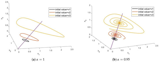
Remark 1.

The equilibrium points are degenerated and set up the ray from the origin to infinity in ${\mathbb{R}}_{+}^3$. Since the quality $H\left(x\right)$ is conserved along the solution of system (1), any solution is towards the line on the plane $S_{H\left(b\right)}$, which is determined by the initial value near the line. Therefore, there are local asymptotic behaviors. However, it is not a strictly asymptotically stable phenomenon. Furthermore, we find that there are solutions spiraling towards the ray for some $\alpha \in (0,1)$ and the initial value b by numerical simulation. In Section 5, we give descriptions of this phenomenon in detail.

5. Numerical Simulations

Consider a system

$$\left\{\begin{array}{c}{D}_t^{\alpha }{x}_1=\left(x_2-x_3\right)x_1\hfill \\ D_t^{\alpha }{x}_2=\left(-x_1+x_3\right)x_2\hfill \\ D_t^{\alpha }{x}_3=\left(x_1-x_2\right)x_3,\hfill \end{array}\right.$$

(19)

with the initial value $x\left(0\right)={(0.35,0.35,0.3)}^{\mathrm{T}}$, where the $D_t^{\alpha }$ is the Caputo fractional derivative with $\alpha \in (0,1]$, $A=\left(\begin{array}{ccc}0& 1& -1\\ -1& 0& 1\\ 1& -1& 0\end{array}\right)$. By Lemma 8, ${\displaystyle \sum _{i=1}^3}{x}_i\equiv 1$; then, the solution to the system (19) with initial value $x\left(0\right)$ contained in the plane

$$S_1:=\left\{v\in {\mathbb{R}}_{+}^3|v={(v_1,v_2,v_3)}^{\mathrm{T}},\sum _{i=1}^3{v}_i=1\right\}.$$

Direct calculations yield that the equilibrium points are

$$\left\{r\in {\mathbb{R}}^3{|r=(s,s,s)}^{\mathrm{T}},s\in \mathbb{R}\right\}$$

and $p={(\frac{1}{3},\frac{1}{3},\frac{1}{3})}^{\mathrm{T}}$ is a unique equilibrium point on plane $S_1$. For $\alpha =1$, any solution curve is closed and around p on $S_1$ by Theorem 2. For $0<\alpha <1$, the solution goes towards p on the plane $S_1$ by Theorem 3.

Next, using Matlab, based on the fractional Adams–Bashforth–Moulton Method (see Appendix C of [31]), numerical simulations are provided to substantiate the theoretical results established in the previous sections of this paper. Next we will monitor the effect of varying order $\alpha$ on the dynamical behavior of the model.

Take the time step as 0.01 and draw the change curve of x with time t in the system (19). Simulations are then run with varying values of $\alpha$ and initial values as in Figure 2, Figure 3, Figure 4, Figure 5, Figure 6 and Figure 7, where the grid-like plane is $S_{H\left(b\right)}$ and $u1={(2,3,5)}^{\mathrm{T}}$, $u2={(4,3,3)}^{\mathrm{T}}$, $u3={(2,4,4)}^{\mathrm{T}}$, $v1={(0.5,0.5,0.3)}^{\mathrm{T}}$, $v2={(1,0.5,0.3)}^{\mathrm{T}}$, $v3={(1,2,0.3)}^{\mathrm{T}}$.

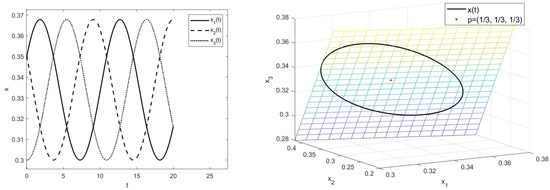
Figure 2. Simulations of system (19) for $\alpha =1$ with initial value $b=(0.35,0.35,0.3)$.

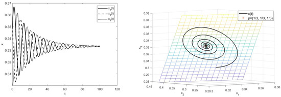
Figure 3. Simulations of system (19) for $\alpha =0.95$ with initial value $b=(0.35,0.35,0.3)$.

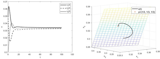
Figure 4. Simulations of system (19) for $\alpha =0.7$ with initial value $b=(0.35,0.35,0.3)$.

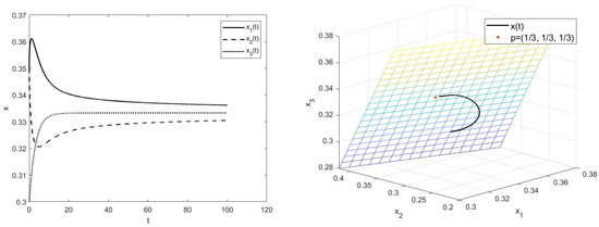
Figure 5. Simulations of system (19) for $\alpha =0.5$ with initial value $b=(0.35,0.35,0.3)$.

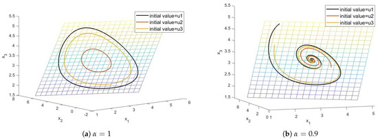
Figure 6. Simulations of system (19) for $\alpha =1$ and $\alpha =0.9$ with initial values $u1,u2$ and $u3$ separately.

Figure 7. Simulations of system (19) for $\alpha =1$ and $\alpha =0.95$ with initial values $v1,v2$ and $v3$ separately (where the rays from the origin are degenerate equilibrium points of system (19)).

We have the following conclusions.

(i)

By Figure 2, Figure 3, Figure 4 and Figure 5, all $x_i\left(t\right)$ have a positive below bound, and all solution curves are on the plane $S_1$ for all times, no matter what $\alpha$.

(ii)

By Figure 6, all solution curves are on one plane if the totals of $x_i\left(0\right)$ are same, no matter what $\alpha$.

(iii)

By Figure 6a and Figure 7a, all solution curves of the first-order system (19) are closed curves and around the equilibrium point.

(iv)

By Figure 7b, all solution curves of the $0.95$-order system (19) go towards the equilibrium point.

The numerical simulation results show that the order does not affect the boundedness but affects the stability.

In addition, an interesting asymptotic behavior can be seen from the Figure 2, Figure 3, Figure 4 and Figure 5, Figure 6b and Figure 7b. To be specific, the equilibrium points set up the ray from the origin to infinity in ${\mathbb{R}}_{+}^3$, and any solution is towards the line on the plane, which is determined by the initial value near the line. Furthermore, there are solutions spiraling towards the ray for some $\alpha \in (0,1)$.

6. Conclusions

Since biological systems have memory properties, fractional differential equations provide an excellent tool in this respect. Thus, this paper studied a class of fractional antisymmetric Lotka–Volterra equations composed of three species under the rock–paper–scissors game rules. The first-order and $0<\alpha <1$-order antisymmetric Lotka–Volterra systems are studied separately. The results show that the order does not affect the boundedness but affects the stability:

(1)

For any $\alpha \in (0,1]$, ${\displaystyle \sum _{i=1}^3}{x}_i\left(t\right)={\displaystyle \sum _{i=1}^3}{x}_i\left(0\right)$ for all times $t>0$, and all $x_i$ bounded away from zero for all times for any choice of $a_{12},a_{23},a_{31}>0$. In the context of population dynamics, this means that the total number of individuals for all species is conserved and all species coexist independently of the predatory efficiency.

(2)

All the solutions of the first-order system are periodic. However, the $0<\alpha <1$-order system can be reduced on a two-dimensional space and the reduced system is asymptotically stable, regardless of how close to zero the order of the derivative used is. This implies that if the equilibrium state is slightly disturbed, as long as the total number of species remains unchanged, it will always return to the original equilibrium state after a long time. This may reflect the memory of the fractional-order system.

References

- Volterra, V. Leçons sur la Théorie Mathématique de la Lutte pourla Vie; Gauthier-Villars: Paris, France, 1931. [Google Scholar]
- Van Kampen, N.G. Stochastic Process in Physics and Chemistry, 3rd ed.; Elsevier: Amsterdam, The Netherlands, 2007. [Google Scholar]
- Zhou, P.; Tang, D.; Xiao, D. On Lotka-Volterra competitive parabolic systems: Exclusion, coexistence and bistability. J. Differ. Equ. 2021, 282, 596–625. [Google Scholar] [CrossRef]
- Ahmed, E.; El-Sayed, A.M.A.; El-Saka, H.A.A. Equilibrium points, stability and numerical solutions of fractional-order predator-prey and rabies models. J. Math. Anal. Appl. 2007, 325, 542–553. [Google Scholar] [CrossRef]
- Nowak, M. Evolutionary Dynamics; Harvard University Press: Cambridge, MA, USA, 2006. [Google Scholar]
- Menezes, J. Antipredator behavior in the rock-paper-scissors model. Phys. Rev. Lett. E 2021, 103, 052216. [Google Scholar] [CrossRef] [PubMed]
- Sinervo, B.; Lively, C. The rock-paper-scissors game and the evolution of alternative male strategies. Nature 1996, 380, 240–243. [Google Scholar] [CrossRef]
- Kirkup, B.; Riley, M. Antibiotic-mediated antagonism leads to a bacterial game of rock-paper-scissors in vivo. Nature 2004, 428, 412–414. [Google Scholar] [CrossRef]
- Wang, Y.; Liu, S. Fractal analysis and control of the fractional Lotka-Volterra model. Nonlinear Dyn. 2019, 95, 1457–1470. [Google Scholar] [CrossRef]
- Zhao, Y.; Sun, S.; Han, Z.; Zhang, M. Positive solutions for boundary value problems of nonlinear fractional differential equations. Appl. Math. Comput. 2011, 217, 6950–6958. [Google Scholar] [CrossRef]
- Elsadany, A.A.; Matouk, A.E. Dynamical behaviors of fractional-order Lotka-Volterra predator-prey model and its discretization. J. Appl. Math. Comput. 2015, 49, 269–283. [Google Scholar] [CrossRef]
- Xu, M.; Sun, S. Positivity for integral boundary value problems of fractional differential equations with two nonlinear terms. J. Appl. Math. Comput. 2019, 59, 271–283. [Google Scholar] [CrossRef]
- Xu, M.; Sun, S.; Han, Z. Solvability for impulsive fractional Langevin equation. J. Appl. Anal. Comput. 2020, 10, 486–494. [Google Scholar] [CrossRef]
- Yavuz, M.; Sene, N. Stability Analysis and Numerical Computation of the Fractional Predator-Prey Model with the Harvesting Rate. Fractal Fract. 2020, 4, 35. [Google Scholar] [CrossRef]
- Podlubny, I. Fractional Differential Equation; Academic Press: New York, NY, USA, 1999. [Google Scholar]
- Kilbas, A.; Srivastava, H.; Trujillo, J. Theory and Applications of Fractional Differential Equations; Elsevier: Amsterdam, The Netherlands, 2006. [Google Scholar]
- Tarasov, V.E. Predator-prey models with memory and kicks: Exact solution and discrete maps with memory. Math. Methods Appl. Sci. 2021, 44, 11514–11525. [Google Scholar] [CrossRef]
- Zhou, P.; Ma, J.; Tang, J. Clarify the physical process for fractional dynamical systems. Nonlinear Dyn. 2020, 100, 2353–2364. [Google Scholar] [CrossRef]
- Tarasov, V.E. Applications in Physics, Part A. In Handbook of Fractional Calculus with Applications; De Gruyter: Berlin, Germany, 2019; Volume 4. [Google Scholar]
- Heymans, N.; Podlubny, I. Physical interpretation of initial conditions for fractional differential equations with Riemann–Liouville fractional derivatives. Rheol. Acta 2006, 45, 765–771. [Google Scholar] [CrossRef]
- Tavassoli, M.H.; Tavassoli, A.; Rahimi, M.R.O. The geometric and physical interpretation of fractional order derivatives of polynomial functions. Differ. Geom. Dyn. Syst. 2013, 15, 93–104. [Google Scholar]
- Ionescu, C.; Lopes, A.; Copot, D.; Machado, J.A.T.; Bates, J.H.T. The role of fractional calculus in modeling biological phenomena: A review. Commun. Nonlinear Sci. Numer. Simul. 2017, 51, 141–159. [Google Scholar] [CrossRef]
- Echenausía-Monroy, J.L.; Gilardi-Velázquez, H.E.; Jaimes-Reátegui, R.; Aboites, V.; Huerta-Cuéllar, G. A physical interpretation of fractional-order-derivatives in a jerk system: Electronic approach. Commun. Nonlinear Sci. Numer. Simul. 2020, 90, 105413. [Google Scholar] [CrossRef]
- Bhalekara, S.; Patilb, M. Singular points in the solution trajectories of fractional order dynamical systems. Chaos 2018, 28, 113123. [Google Scholar] [CrossRef]
- El-Dib, Y.; Elgazery, N. Effect of fractional derivative properties on the periodic solution of the nonlinear oscillations. Fractals 2020, 28, 2050095. [Google Scholar] [CrossRef]
- Monroy, J.; Cuellar, G.; Reategui, R.; García-López, J.H.; Aboites, V.; Cassal-Quiroga, B.B.; Gilardi-Velázquez, H.E. Multistability Emergence through Fractional-Order-Derivatives in a PWL Multi-Scroll System. Electronics 2020, 9, 880. [Google Scholar] [CrossRef]
- Daftardar-Gejji, V.; Bhalekar, S. Chaos in fractional ordered Liu system. Comput. Math. Appl. 2010, 59, 1117–1127. [Google Scholar] [CrossRef]
- Li, C.; Chen, G. Chaos, hyperchaos in the fractional-order Rossler equations. Phys. A Stat. Mech. Appl. 2004, 341, 55–61. [Google Scholar] [CrossRef]
- Moustafa, M.; Abdullah, F.A.; Shafie, S. Dynamical behavior of a fractional-order prey-predator model with infection and harvesting. J. Appl. Math. Comput. 2022, 68, 4777–4794. [Google Scholar] [CrossRef]
- Das, S.; Mahato, S.; Mondal, A.; Kaslik, E. Emergence of diverse dynamical responses in a fractional-order slow-fast pest-predator model. Nonlinear Dyn. 2023, 111, 8821–8836. [Google Scholar] [CrossRef]
- Kai, D. The Analysis of Fractional Differential Equations; Springer: Berlin/Heidelberg, Germany, 2010. [Google Scholar]
- Li, C.; Ma, Y. Fractional dynamical system and its linearization theorem. Nonlinear Dyn. 2013, 71, 621–633. [Google Scholar] [CrossRef]
Disclaimer/Publisher’s Note: The statements, opinions and data contained in all publications are solely those of the individual author(s) and contributor(s) and not of MDPI and/or the editor(s). MDPI and/or the editor(s) disclaim responsibility for any injury to people or property resulting from any ideas, methods, instructions or products referred to in the content. |
© 2023 by the author. Licensee MDPI, Basel, Switzerland. This article is an open access article distributed under the terms and conditions of the Creative Commons Attribution (CC BY) license (https://creativecommons.org/licenses/by/4.0/).