A Non-Convex Hybrid Overlapping Group Sparsity Model with Hyper-Laplacian Prior for Multiplicative Noise

Abstract

Multiplicative noise removal is a quite challenging problem in image denoising. In recent years, hyper-Laplacian prior information has been successfully introduced in the image denoising problem and significant denoising effects have been achieved. In this paper, we propose a new hybrid regularizer model for removing multiplicative noise. The proposed model consists of the non-convex higher-order total variation and overlapping group sparsity on a hyper-Laplacian prior regularizer. It combines the advantages of the non-convex regularization and the hybrid regularization, which may simultaneously preserve the fine-edge information and reduce the staircase effect at the same time. We develop an effective alternating minimization method for the proposed nonconvex model via an alternating direction method of multipliers framework, where the majorization–minimization algorithm and the iteratively reweighted algorithm are adopted to solve the corresponding subproblems. Numerical experiments show that the proposed model outperforms the most advanced model in terms of visual quality and certain image quality measurements.

1. Introduction

Image noise removal is an extremely significant pre-processing step in the image-processing task. Multiplicative noise frequently presents in synthetic aperture radars, ultrasound imaging, and laser images, which causes image quality degradation. Therefore, the problem of multiplicative noise removal is very important. Mathematically, the degraded observation image model with multiplicative noise is represented as

$$\begin{array}{c}\hfill f=u·\eta ,\end{array}$$

(1)

where f denotes the degraded image, u denotes an original image, and the multiplicative noise $\eta$ follows a Gamma distribution with the probability density function (PDF):

$$\begin{array}{ccc}\hfill P(\eta ,L)=\frac{L^L}{\Gamma \left(L\right)}{\eta }^{L-1}{e}^{-L\eta },& \hfill & \hfill L>1,\end{array}$$

(2)

where $\Gamma (·)$ is a Gamma function, and L is an integer to represent the noise level. The smaller the value of L, the more severe the damage of the noise becomes. The mean value of $\eta$ is 1 and the variance of $\eta$ is $1/L$.

Variational methods are effectively used for removing multiplicative noise. Among these variational methods, the total variation (TV)-based method is the best known and the most popular and efficient, since it can effectively preserve the image edges while suppressing noise [1,2]. In [3], a famous TV-based multiplicative noise removal model (RLO model) with two equality constraints was first designed by Rudin et al., which can be addressed by a gradient projection algorithm. Unfortunately, the RLO model can only deal with the noise that follows Gaussian distribution and cannot yield satisfactory recovery results for Gamma distribution. For the removal of the multiplicative Gamma noise, Aubert and Aujol [4] proposed the following variational model (the AA model) based on total variational regularization:

$$\underset{u}{\min }\left\{\begin{array}{c}\hfill \alpha ⟨logu+\frac{f}{u},1⟩+{\parallel \nabla u\parallel }_1\end{array}\right\},$$

(3)

where $\alpha$ is a positive regular parameter. The problem (3) is a non-convex optimization problem, so it is difficult to obtain a globally optimal solution. To overcome the effects of non-convex objective functions, many researchers have considered many convex models over the past decade. In [5,6,7], the authors used logarithm transforming to derive the corresponding strictly convex model:

$$\underset{z}{\min }\left\{\begin{array}{c}\hfill \alpha ⟨z+f{e}^{-z},1⟩+{\parallel \nabla z\parallel }_1\end{array}\right\},$$

(4)

where $z=logu$. In addition, Steidl and Teuber [8] chose to use the I-divergence as the data fidelity term of the objective function and proposed a convex optimization model:

$$\underset{z}{\min }\left\{\begin{array}{c}\hfill \alpha ⟨z-flogz,1⟩+{\parallel \nabla z\parallel }_1\end{array}\right\}.$$

(5)

The advantage of the above model is that a nonlinear log transformation is not required. By introducing an overlapping group sparsity total variation regularization term into an I-divergence data fidelity term, Liu et al. [9] proposed the convex variational model (“OGSTVD” for short) for removing multiplicative noise:

$$\underset{z}{\min }\left\{\begin{array}{c}\hfill \alpha ⟨logz+\frac{f}{z},1⟩+\varphi (\nabla z)\end{array}\right\},$$

(6)

where the $\varphi (\nabla z)$ is the OGSTV regular function. They also illustrate the effectiveness of their model in image restoration by some numerical results.

All of the above models are TV-based convex regularizer ones. Although many studies showed that TV-based models have a good performance in keeping sharp edges, they tend to produce undesired staircase effects. To compensate for these shortcomings, many higher-order TV regularization terms are also proposed. By combining the first-order and second-order TV, Liu [10] proposed a hybrid regularization model for multiplicative noise removal. Shama et al. [11] proposed a model based on second-order total generalized variational regularization (TGV) to remove multiplicative noise. Influenced by model (4), Lv [12] proposed a TGV-based model (M-TGV for short) for multiplicative noise removal with multilook M. To obtain high-quality recovered images, some non-convex regularizers were introduced into the variational models. The non-convex regularizer can effectively smooth the homogeneous region of the image while preserving the edge details of the image. Chartrand [13] gives a non-convex optimization problem whose objective function is the $l_p$ norm, giving an arbitrary sparse signal under the theoretical constitutability condition. The models with non-convex regularizers can also be found in [14,15,16,17]. Extensive studies show that the models with non-convex regularizers have outperformed the models with convex regularizers in preserving the edges of the image.

Natural image gradients obey a heavy-tailed distribution, and hyper-Laplacian (HL) prior is more approximated to the heavy-tailed distribution than the Gaussian or Laplacian prior. Krishnan et al. [18] proposed a fast non-blurred image deblurring method based on a super-Laplace prior. Many scholars studied multispectral image denoising [19,20,21,22,23] based on the global spectral structure of the HL prior regularization term. Shi et al. [24] combined the OGSTV and HL prior regularizer (OGSHL) to remove Gaussian noise. They showed that their proposed model can effectively utilize more texture information and find a satisfying balance between suppressing staircase effects and recovering the structure information.

Using the above strategy as inspiration, we develop a novel hybrid regularization model to eliminate multiplicative noise. The model combines the advantages of nonconvex regularization and OGSHL regularization. More specifically, the model can be expressed as follows:

$$\underset{z}{\min }\left\{\begin{array}{c}\hfill \alpha ⟨z-flogz,1⟩+{\varphi }_{OH}(\nabla z)+\omega {\parallel {\nabla }^{2}z\parallel }_p^p\end{array}\right\},$$

(7)

where the ${\varphi }_{OH}(\nabla z)$ is the OGSHL regular function and $0<p<1$. According to what we know, there has been no attempt to combine overlapping group sparsity on a hyper-Laplacian (OGSHL) prior with higher-order non-convex total variation regularizers to remove multiplicative noise. The main contributions of this paper are summarized as follows: (1) We propose a new hybrid regular denoising model that combines a non-convex higher-order total variation and overlapping group sparsity total variation on a hyper-Laplacian prior. It can suppress the staircase effect while retaining more image detail information. (2) To make the optimization model easy to handle, we propose an efficient alternating minimization method. (3) The experimental results verify that the proposed method outperforms many state-of-the-art methods.

The remaining portions of this article are outlined below. Section 2 introduces the definitions of the higher-order TV and an OGSHL. In Section 3, based on the alternating direction method of multipliers, we develop an efficient algorithm to solve the corresponding multiplicative removal problem. In Section 4, numerical results show the effectiveness of the proposed method. In Section 5, a summary of the paper is presented.

2. Preliminaries

We present some relevant background knowledge in this section.

2.1. Second-Order TV

For any $z\in R^{m\times n}$, $z_{i,j}$ denotes the intensity value of z at pixel $(i,j)$ for $i=1,\cdots ,m,j=1,\cdots ,n$. The definitions of the first-order forward and backward difference operators are given below:

$$\begin{gathered} \hspace{1em}\begin{array}{cc}\hfill {\left({\nabla }_x^{+}z\right)}_{i,j}=\left\{\begin{array}{ccc}{z}_{i+1,j}-z_{i,j}\hfill & & i<m,\hfill \\ z_{1,j}-z_{n,j}\hfill & & i=m,\hfill \end{array}\right.& \end{array}\hspace{1em}\begin{array}{cc}\hfill {\left({\nabla }_y^{+}z\right)}_{i,j}=\left\{\begin{array}{ccc}{z}_{i,j+1}-z_{i,j}\hfill & & j<n,\hfill \\ z_{i,1}-z_{i,n}\hfill & & j=n,\hfill \end{array}\right.& \end{array} \\ {\left({\nabla }_x^{-}z\right)}_{i,j}=\left\{\begin{array}{ccc}{z}_{1,j}-z_{n,j}\hfill & & i=1,\hfill \\ z_{i+1,j}-z_{i,j}\hfill & & i>1.\hfill \end{array}\right.\hspace{1em}\hspace{1em} {\left({\nabla }_y^{-}z\right)}_{i,j}=\left\{\begin{array}{ccc}{z}_{i,1}-z_{i,n}\hfill & & j=1,\hfill \\ z_{i,j+1}-z_{i,j}\hfill & & j>1.\hfill \end{array}\right. \end{gathered}$$

By introducing the operators above, the second-order differential operator is expressed as

$$\begin{gathered} \begin{array}{c}{\left({\nabla }_{xx}^{-+}z\right)}_{i,j}={\left({\nabla }_x^{-}\left({\nabla }_x^{+}z\right)\right)}_{i,j},\hfill \end{array}\begin{array}{c}{\left({\nabla }_{yy}^{-+}z\right)}_{i,j}={\left({\nabla }_y^{-}\left({\nabla }_y^{+}z\right)\right)}_{i,j},\hfill \end{array} \\ \begin{array}{c}{\left({\nabla }_{xy}^{++}z\right)}_{i,j}={\left({\nabla }_x^{+}\left({\nabla }_y^{+}z\right)\right)}_{i,j},\hfill \end{array}\begin{array}{c}{\left({\nabla }_{yx}^{++}z\right)}_{i,j}={\left({\nabla }_y^{+}\left({\nabla }_x^{+}z\right)\right)}_{i,j},\hfill \end{array} \end{gathered}$$

$$\begin{array}{c}{\parallel \nabla z\parallel }_1={\displaystyle \sum _{i,j}}\mid {(\nabla z)}_{i,j}\mid ={\displaystyle \sum _{i,j}}\sqrt{{\left({\nabla }_x^{+}z\right)}_{i,j}^2+{\left({\nabla }_y^{+}z\right)}_{i,j}^2}.\hfill \\ \parallel {\nabla }^2{z\parallel }_1={\displaystyle \sum _{i,j}}\mid {\left({\nabla }^{2}z\right)}_{i,j}\mid ={\displaystyle \sum _{i,j}}\sqrt{{\left({\nabla }_{xx}^{-+}z\right)}_{i,j}^2+{\left({\nabla }_{xy}^{++}z\right)}_{i,j}^2+{\left({\nabla }_{yx}^{++}z\right)}_{i,j}^2+{\left({\nabla }_{yy}^{-+}z\right)}_{i,j}^2}.\hfill \end{array}$$

2.2. Overlapping Group Sparsity on Hyper-Laplacian Prior

With respect to the two-dimensional image matrix $z\in {\mathbb{R}}^{n\times n}$, a $K\times K$-point group is defined in [25] as

$$\begin{array}{c}\hfill {\tilde{z}}_{(i,j),K}=\left[\begin{array}{ccc}z(i-m_1,j-m_1)& \cdots & z(i-m_1,j+m_2)\\ z(i-m_1+1,j-m_1)& \cdots & z(i-m_1+1,j+m_2)\\ ⋮& \ddots & ⋮\\ z(i+m_2,j-m_1)& \cdots & z(i+m_2,j+m_2)\end{array}\right]\in R^{K\times K},\end{array}$$

where $m_1=⌊\frac{K-1}{2}⌋$ and $m_2=⌊\frac{K}{2}⌋$, $⌊t⌋$ denotes the nearest integer that is not nearer than t. It is clear that ${\tilde{z}}_{(i,j),K}$ can be seen as a square block of continuous $K\times K$ sampling of z. According to the dictionary parsimonious search, Liu et al. [25] arranged $\tilde{z}$ as a set of column vectors z, i.e., $z_{(i,j),K}={\tilde{z}}_{(i,j),K}(:)$. Then, the two-dimensional overlapping group sparsity regularizer is defined as

$$\begin{array}{c}\hfill \phi \left(z\right)=\sum _{i,j=1}^n\parallel z_{(i,j),K}{\parallel }_2=\sum _{i,j=1}^n\sqrt{\sum _{k_1,k_2=-m_1}^{m_2}\mid z(i+k_1,j+k_2){\mid }^2}.\end{array}$$

From the above definition, the definition of the overlapping group sparse total variation $\varphi (\nabla z)$ can be expressed as

$$\begin{array}{c}\hfill \varphi \left(\nabla z\right)=\phi \left({\nabla }_x^{+}z\right)+\phi \left({\nabla }_y^{+}z\right).\end{array}$$

The hyper-Laplacian prior theory has recently attracted much attention since it offers a benign approximation to the heavy-tailed distribution of natural image gradients. Kyongson et al. [26] define the OGS-HL regularizer ${\varphi }_{OH}(\nabla z)$ by

$$\begin{array}{c}\hfill {\varphi }_{OH}\left(\nabla z\right)={\phi }_{OH}\left({\nabla }_x^{+}z\right)+{\phi }_{OH}\left({\nabla }_y^{+}z\right).\end{array}$$

with

$$\begin{array}{c}\hfill {\phi }_{OH}\left(z\right)=\sum _{i,j=1}^n\parallel \mid z_{(i,j),K}{\mid }^r{\parallel }_2=\sum _{i,j=1}^n\sqrt{\sum _{k_1,k_2=-m_1}^{m_2}\mid z(i+k_1,j+k_2){\mid }^{2r}},\end{array}$$

where $|z_{(i,j),K}{|}^r$ is a vector whose elements are the r-th power of the absolute value of the corresponding element, r is the scale parameter of the hyper-Laplacian distribution, $0<r<1$, see [26]. If $r=1$, ${\varphi }_{OH}\left(z\right)=\varphi \left(z\right)$.

3. Proposed Method with Adaptive Parameter Adjustment

In the framework of the alternating direction method of multipliers (ADMM), the variable splitting technique is used to solve the proposed model. We first introduce new auxiliary variables $w,v$, and q. Then, the original unconstrained optimization problem (7) can be converted into an equivalent constrained minimization problem as follows:

$$\begin{array}{cc}\hfill & \underset{z,w,v,q}{\min }\alpha ⟨w-flogw,1⟩+{\varphi }_{OH}\left(v\right)+\omega {\parallel q\parallel }_p^p,\hfill \\ \hfill & s.t.w=z,v=\nabla z,q={\nabla }^{2}z.\hfill \end{array}$$

(8)

We define the corresponding augmented Lagrangian function of (8) as follows:

$$\begin{array}{cc}\hfill & {\mathcal{L}}_A(z,w,v,q;{\mu }_1,{\mu }_2,{\mu }_3)\hfill \\ \hfill =& \alpha ⟨w-flogw,1⟩+{\varphi }_{OH}\left(v\right)+{\omega \parallel q\parallel }_p^p-{\mu }_1^T(w-z)+\frac{{\beta }_1}{2}{\parallel w-z\parallel }_2^2\hfill \\ \hfill & -{\mu }_2^T(v-\nabla z)+\frac{{\beta }_2}{2}{\parallel v-\nabla z\parallel }_2^2-{\mu }_3^T(q-{\nabla }^{2}z)+\frac{{\beta }_3}{2}{\parallel q-{\nabla }^{2}z\parallel }_2^2,\hfill \\ \hfill =& \alpha ⟨w-flogw,1⟩+{\varphi }_{OH}\left(v\right)+\omega {\parallel q\parallel }_p^p\hfill \\ \hfill & +\frac{{\beta }_1}{2}\parallel w-z-\frac{{\mu }_1}{{\beta }_1}{\parallel }_2^2+\frac{{\beta }_2}{2}\parallel v-\nabla z-\frac{{\mu }_2}{{\beta }_2}{\parallel }_2^2+\frac{{\beta }_3}{2}\parallel q-{\nabla }^{2}z-\frac{{\mu }_3}{{\beta }_3}{\parallel }_2^2,\hfill \end{array}$$

where ${\beta }_i(i=1,2,3)$ are positive penalty parameters, and ${\mu }_i(i=1,2,3)$ are the Lagrange multipliers, respectively. The optimal solution of (8) can be obtained by finding the saddle point of ${\mathcal{L}}_A(z,w,v,q;{\mu }_1,{\mu }_2,{\mu }_3)$ under the framework of the ADMM. We alternately solve the following subproblems in the framework:

$$\left\{\begin{array}{c}{w}^{k+1}=\underset{w}{\mathrm{argmin}}{\mathcal{L}}_A(z^k,w,v^k,q^k;{\mu }_1^k,{\mu }_2^k,{\mu }_3^k),\hfill \\ q^{k+1}=\underset{q}{\mathrm{argmin}}{\mathcal{L}}_A(z^k,w^{k+1},v^k,q;{\mu }_1^k,{\mu }_2^k,{\mu }_3^k),\hfill \\ v^{k+1}=\underset{v}{\mathrm{argmin}}{\mathcal{L}}_A(z^k,w^{k+1},v,q^{k+1};{\mu }_1^k,{\mu }_2^k,{\mu }_3^k),\hfill \\ z^{k+1}=\underset{z}{\mathrm{argmin}}{\mathcal{L}}_A(z,w^{k+1},v^{k+1},q^{k+1};{\mu }_1^k,{\mu }_2^k,{\mu }_3^k),\hfill \end{array}\right.$$

and the Lagrange multiplier parameters are updated as follows:

$$\left\{\begin{array}{c}{\mu }_1^{k+1}={\mu }_1^k-{\beta }_1(w^{k+1}-z^{k+1}),\hfill \\ {\mu }_2^{k+1}={\mu }_2^k-{\beta }_2(v^{k+1}-\nabla z^{k+1}),\hfill \\ {\mu }_3^{k+1}={\mu }_3^k-{\beta }_3(q^{k+1}-{\nabla }^2{z}^{k+1}).\hfill \end{array}\right.$$

Firstly, fixing $z=z^k$, $v=v^k$ and $q=q^k$, the w-subproblem is following optimization problem:

$$\begin{array}{cc}\hfill w^{k+1}=\underset{w}{\mathrm{argmin}}& {\mathcal{L}}_A(w,q^k,v^k,z^k;{\mu }_1^k,{\mu }_2^k,{\mu }_3^k)\hfill \\ \hfill =\underset{w}{\mathrm{argmin}}& \alpha ⟨w-flogw,1⟩+\frac{{\beta }_1}{2}\parallel w-z^k-\frac{{\mu }_1^k}{{\beta }_1}{\parallel }_2^2.\hfill \end{array}$$

(9)

Using the Euler–Lagrange equation of (9), we can obtain the optimal solution of the w subproblem:

$$\begin{array}{c}\hfill \alpha (1-\frac{f}{w})+{\beta }_1(w-z^k-\frac{{\mu }_1^k}{{\beta }_1})=0.\end{array}$$

Then, the solution of w is

$$\begin{array}{c}\hfill w^{k+1}=\frac{1}{2}\{(z^k+\frac{{\mu }_1^k}{{\beta }_1}-\frac{\alpha }{{\beta }_1})+\sqrt{{(z^k+\frac{{\mu }_1^k}{{\beta }_1}-\frac{\alpha }{{\beta }_1})}^2+\frac{4\alpha f}{{\beta }_1}}\}.\end{array}$$

(10)

Secondly, the q-subproblem is equivalent to the following nonconvex optimization problem:

$$\begin{array}{cc}\hfill q^{k+1}=& \underset{q}{\mathrm{argmin}}{\mathcal{L}}_A(z^k,v^k,w^{k+1},q;{\mu }_1^k,{\mu }_2^k,{\mu }_3^k)\hfill \\ \hfill =& \underset{q}{\mathrm{argmin}}{\omega \parallel q\parallel }_p^p+\frac{{\beta }_3}{2}\parallel q-{\nabla }^2{z}^k-\frac{{\mu }_3^k}{{\beta }_3}{\parallel }_2^2.\hfill \end{array}$$

(11)

The q-subproblem (11) is rewritten as

$$\begin{array}{c}\hfill q^{k+1}=\underset{q}{\mathrm{argmin}}\tau {\parallel q\parallel }_p^p+\frac{1}{2}\parallel q-y^k{\parallel }_2^2,\end{array}$$

(12)

where $y^k={\nabla }^2{z}^k+\frac{{\mu }_3^k}{{\beta }_3},\tau =\omega /{\beta }_3$. In this paper, we adopted the the iterative re-weighted ${\ell }_1$ algorithm (IRL1) method [27] to solve this non-convex ${\ell }_p$ regularized problem (12). As in [27], we approximated the nonconvex minimization (12) to the following weighted ${\ell }_1$ problem:

$$\begin{array}{c}\hfill q^{k+1}=\underset{q}{\mathrm{argmin}}\sum _i{\eta }_i\mid q_i\mid +\frac{1}{2}\parallel q-y^k{\parallel }_2^2,\end{array}$$

(13)

where $\eta$ is a weight vector with each component of ${\eta }_i=\frac{\tau p}{{(\mid q_i^k\mid +ϵ)}^{1-p}}$ and $ϵ>0$ is a number close to zero. The minimization problem (13) has a optimal solution and is obtained by the one-dimensional shrink operator:

$$\begin{array}{c}\hfill q^{k+1}=max\left\{\mid y^k\mid -{\eta }_i,0\right\}\circ sgn\left(y^k\right).\end{array}$$

(14)

Thirdly, the minimization of v-subproblem can be expressed as

$$\begin{array}{cc}\hfill v^{k+1}& =\underset{v}{\mathrm{argmin}}{\mathcal{L}}_A(z^k,w^{k+1},v,q^{k+1};{\mu }_1^k,{\mu }_2^k,{\mu }_3^k)\hfill \\ \hfill & =\underset{v}{\mathrm{argmin}}{\varphi }_{OH}\left(v\right)+\frac{{\beta }_2}{2}\parallel v-\nabla z^k-\frac{{\mu }_2^k}{{\beta }_2}{\parallel }_2^2.\hfill \end{array}$$

(15)

By using the majorization–minimization (MM) [26], the problem (15) can be iteratively solved as

$$v^{k+1}=arg\underset{v}{min}\frac{{\beta }_2}{2}\parallel v-v_0{\parallel }_2^2+\frac{r}{2}\parallel \Lambda \left(v^k\right)\left(\mid v^k{\mid }^{r-1}\odot \mid v\mid \right){\parallel }_2^2,$$

(16)

where $\Lambda \left(v\right)$ is a diagonal matrix whose elements of each diagonal are

$${[\Lambda \left(v\right)]}_{l,l}=\sqrt{\sum _{i,j=-m_1}^{m_2}({\sum _{k_1,k_2=-m_1}^{m_2}\mid v(s-i+k_1,t-j+k_2){\mid }^{2r})}^{\frac{1}{2}}},$$

with $l=(s-1)n+t$, for $s,t=1,\cdots ,n,$ and $r\in (0,1)$, ⊙ denotes element-wise multiplication, $v_0=\nabla z^k+\frac{{\mu }_2^k}{{\beta }_2}$. Therefore, the explicit optimal solution to the v subproblem is given as follows:

$$\begin{array}{c}\hfill v^{k+1}={\left(I+\frac{r}{{\beta }_2}\Lambda {\left(v^k\right)}^T\Lambda \left(v^k\right)S\left(v^k\right)\right)}^{-1}{v}_0,\end{array}$$

(17)

where I denotes an $n^2$ identity matrix, and $S\left(v\right)=diag(\mid v{\mid }^{2r-2})$.

Finally, the z subproblem can be simplified as

$$\begin{array}{cc}\hfill z^{k+1}=\underset{z}{\mathrm{argmin}}& {\mathcal{L}}_A(z,v^{k+1},w^{k+1},q^{k+1};{\mu }_1^k,{\mu }_2^k,{\mu }_3^k)\hfill \\ \hfill =\underset{z}{\mathrm{argmin}}& \frac{{\beta }_1}{2}\parallel w^{k+1}-z-\frac{{\mu }_1^k}{{\beta }_1}{\parallel }_2^2+\frac{{\beta }_2}{2}\parallel v^{k+1}-\nabla z-\frac{{\mu }_2^k}{{\beta }_2}{\parallel }_2^2\hfill \\ \hfill & +\frac{{\beta }_3}{2}\parallel q^{k+1}-{\nabla }^{2}z-\frac{{\mu }_3^k}{{\beta }_3}{\parallel }_2^2,\hfill \end{array}$$

(18)

By differentiating the minimization problem (18) directly, its optimal solution can be obtained from the following Euler–Lagrange equation:

$$\begin{array}{cc}\hfill & \left({\beta }_{1}I+{\beta }_2{\nabla }^T\nabla +{\beta }_3{\left({\nabla }^2\right)}^T{\nabla }^2\right)z^{k+1}\hfill \\ \hfill =& {\beta }_1(w^{k+1}-\frac{{\mu }_1^k}{{\beta }_1})+{\beta }_2{\nabla }^T(v^{k+1}-\frac{{\mu }_2^k}{{\beta }_2})+{\beta }_3{({\nabla }^2)}^T(q^{k+1}-\frac{{\mu }_3^k}{{\beta }_3}).\hfill \end{array}$$

(19)

By using the fast Fourier transform, the optimal solution of (19) can be given as

$$\begin{array}{c}\hfill z^{k+1}={\mathcal{F}}^{-1}(\frac{\mathcal{F}({\beta }_1(w^{k+1}-\frac{{\mu }_1^k}{{\beta }_1})+{\beta }_2{\nabla }^T(v^{k+1}-\frac{{\mu }_2^k}{{\beta }_2})+{\beta }_3{({\nabla }^2)}^T(q^{k+1}-\frac{{\mu }_3^k}{{\beta }_3}))}{\mathcal{F}({\beta }_{1}I+{\beta }_2{\nabla }^T\nabla +{\beta }_3{({\nabla }^2)}^T{\nabla }^2)}).\end{array}$$

(20)

We give a detailed description of the proposed method (named Algorithm 1: NHOGSHL) for removing multiplicative noise as follows.

Algorithm 1: NHOGSHL for image restoration under multiplicative noise

Input: $f,\alpha ,\omega ,{\beta }_1,{\beta }_2,{\beta }_3,K,Niter,\epsilon ={10}^{-5}.$

Initialize: $k=0,z^0=f,t_0=1,{\mu }_1^0=\mathbf{0},{\mu }_2^0=\mathbf{0},{\mu }_3^0=\mathbf{0}.$

While $\frac{\Vert z^{k+1}-z^k{\parallel }_2}{\parallel z^k{\parallel }_2}<\epsilon$

(1): Update $w^{k+1}$ by solving (10);

(2): Update $q^{k+1}$ by solving (14);

(3): Update $v^{k+1}$ by solving (17);

(4): Update $z^{k+1}$ by solving (20);

(5): Update ${\mu }_1^{k+1},{\mu }_2^{k+1},{\mu }_3^{k+1}$ $$\begin{array}{cc}\hfill & {\mu }_1^{k+1}={\mu }_1^k-{\beta }_1(w^{k+1}-z^{k+1}),\hfill \\ \hfill & {\mu }_2^{k+1}={\mu }_2^k-{\beta }_2(v^{k+1}-\nabla z^{k+1}),\hfill \\ \hfill & {\mu }_3^{k+1}={\mu }_3^k-{\beta }_3(q^{k+1}-{\nabla }^2{z}^{k+1}).\hfill \end{array}$$    End

Output $z^{k+1}.$

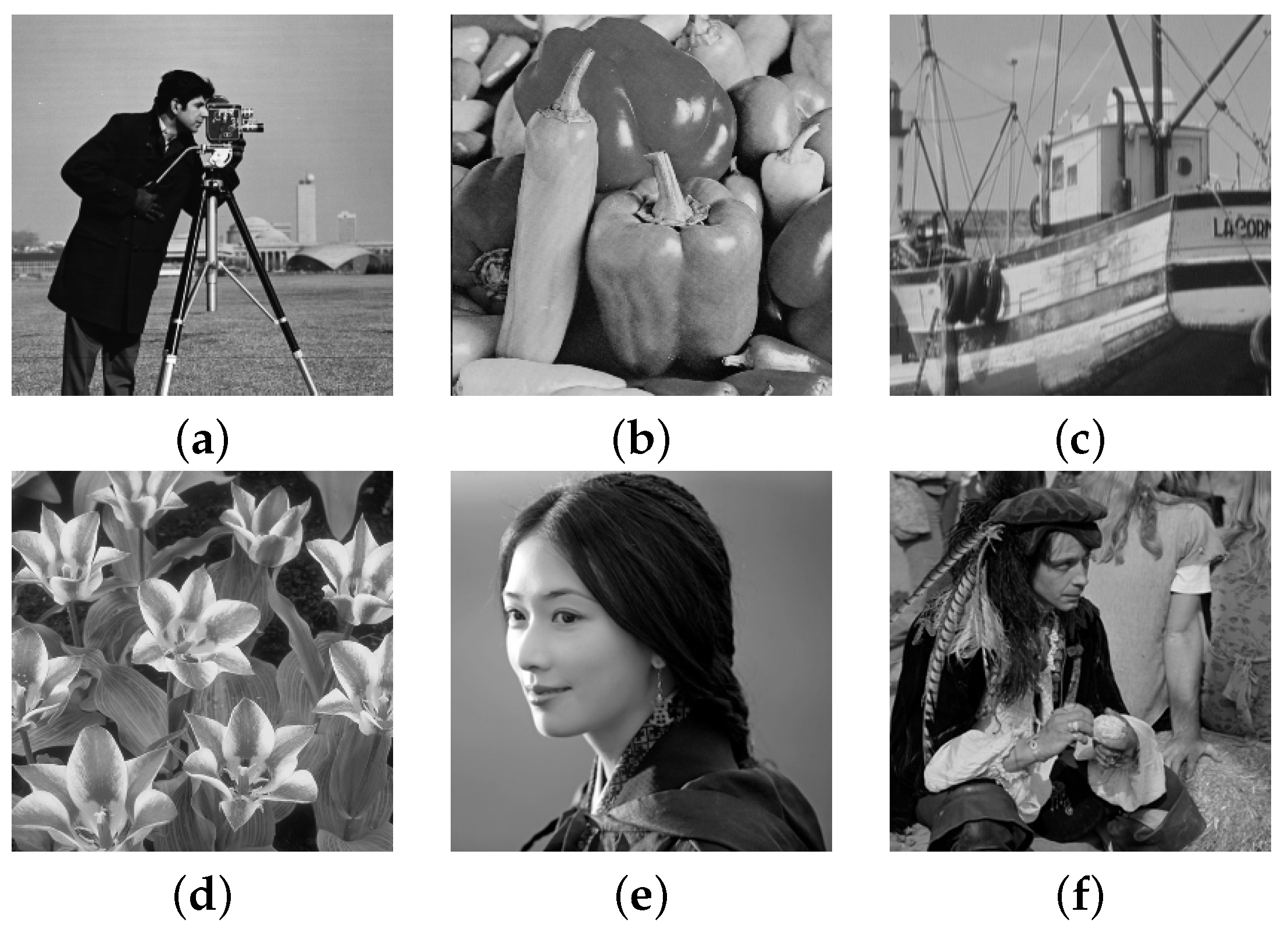
4. Numerical Experiments

In this section, we illustrate the effectiveness of the NHOGSHL model (7), compared with the following three models: the CONVEX model in [28], the OGSTVD model in [9], and the M-TGV model in [12]. The six gray-scale images shown in Figure 1, whose sizes are all $256\times 256$, were used in the experiment. All the experimental results of this article were obtained under MATLAB R2014a running Matlab code on a PC equipped with 4.00 GB RAM and Intel(R) Core(TM) i5-6500U CPU(3.20 GHz). In addition to selecting the peak signal-to-noise ratio (PSNR, unit: dB) as a quantitative and qualitative index to measure image quality, the structural similarity index measurement (SSIM) [29] was also calculated to assess the visual quality. They are defined as follows:

$$\begin{array}{c}\hfill PSNR=10lo{g}_{10}\left(\frac{{255}^2}{\frac{1}{n^2}{\Vert z^0-z\Vert }_2^2}\right),\end{array}$$

where $z^0$ denotes the original image and z denotes the recovered clean image.

$$\begin{array}{c}\hfill SSIM=\frac{(2{\mu }_{z^0}{\mu }_z+c_1)(2{\sigma }_{z^{0}z}+c_2)}{({\mu }_{z^0}^2+{\mu }_z^2+c_1)({\sigma }_{z^0}^2+{\sigma }_z^2+c_2)},\end{array}$$

where ${\mu }_{z^0}$ and ${\mu }_z$ are the means of the $z^0$ and z, respectively. ${\sigma }_{z^0}^2$ and ${\sigma }_z^2$ represent the standard deviation of the $z^0$ and z, respectively, and ${\sigma }_{z^{0}z}$ represents the covariance of the $z^0$ and z. $c_1$ and $c_2$ are normal numbers with denominator values close to zero. As the PSNR value is higher, the SSIM value is nearer to 1, and the image recovery is better. In all experiments, the stop criterion is set to

$$\begin{array}{c}\hfill \frac{\Vert z^{k+1}-z^k{\parallel }_2}{\parallel z^k{\parallel }_2}<{10}^{-5}.\end{array}$$

Figure 1. Test images: (a) Camera, (b) Peppers, (c) Boats, (d) Tulips, (e) Lin, (f) Man.

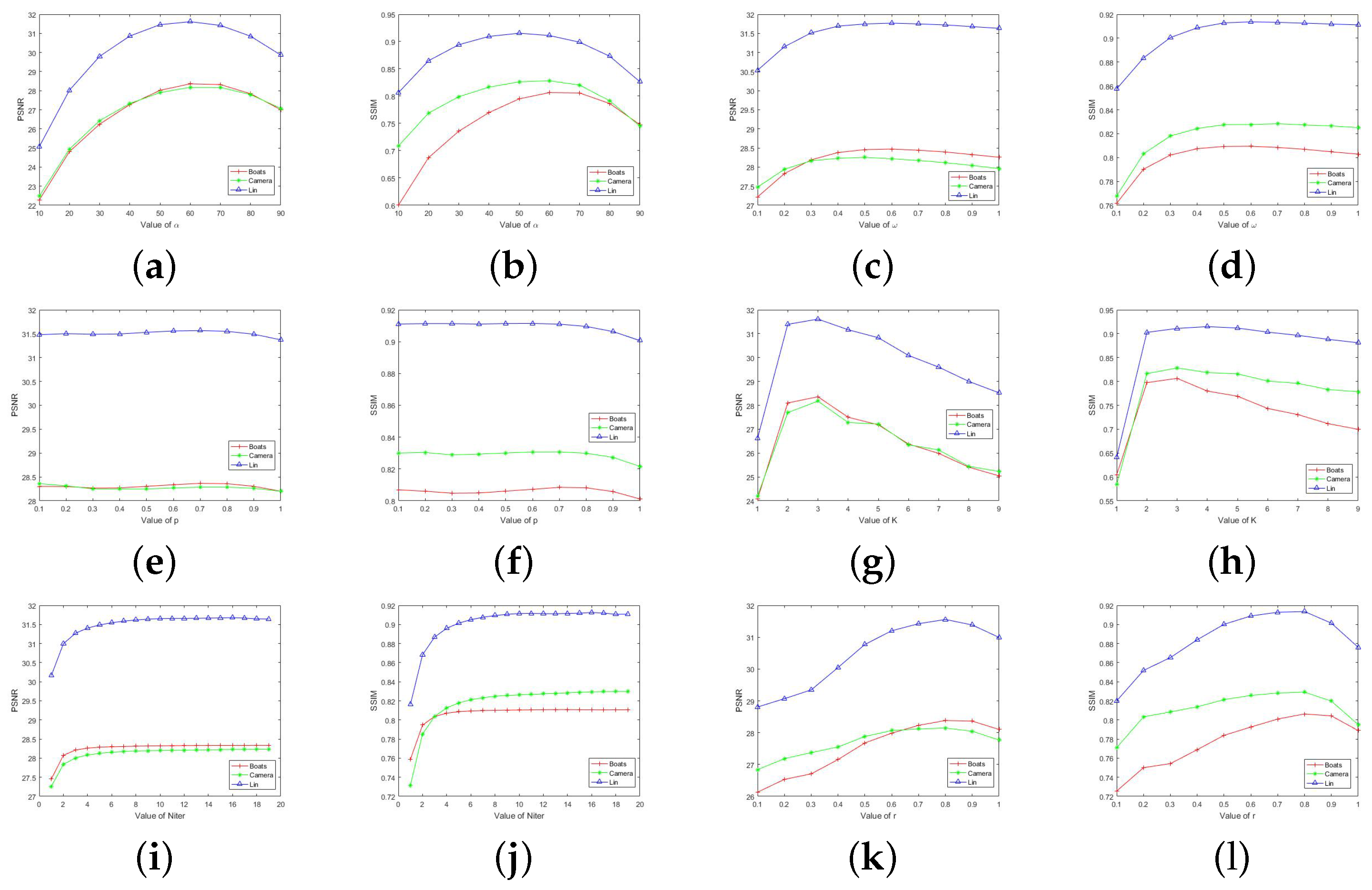
4.1. Parameters Setting

In this section, we will describe in detail the best values for the different parameters $\alpha ,\omega ,p,K,Niter$, and r. We take three images of “Boats”, “Camera”, and “Lin” as examples to illustrate the process of parameter selection. We added multiplicative noise level with $L=20$ to these three images.

First, we assume that the other parameters are known and let $\alpha$ change between 10 and 90, so as to determine the optimal value of parameter $\alpha$. The variation in PSNR and SSIM with the value of parameter $\alpha$ is plotted in Figure 2. We can see that when the $\alpha$ value is around 60, the proposed method has the best effect. Similarly, the optimal value of $\omega$ can be obtained. When the parameter $\omega$ is around 0.7, both PSNR and SSIM reach the maximum. Therefore, the parameter $\omega$ was set to $0.7$ in the following experiments.

Figure 2. (a–l) The PSNR and SSIM values with respect to the parameters $\alpha$, $\omega$, p, K, $Niter$, and r.

Next, Figure 2 plots the PSNR and SSIM and the relationship between the parameters p and r. From Figure 2, we can see that the optimal results can be obtained when $p\in (0.5,0.7)$ and $r=0.8$. Therefore, we set $p=0.6$ and $r=0.8$.

Finally, Figure 2 shows that the optimal value of the group size $K=3$. The experimental results tend to converge to the optimum when the number of iterations is $Niter>10$. Therefore, we set $Niter=10$ in our experiments.

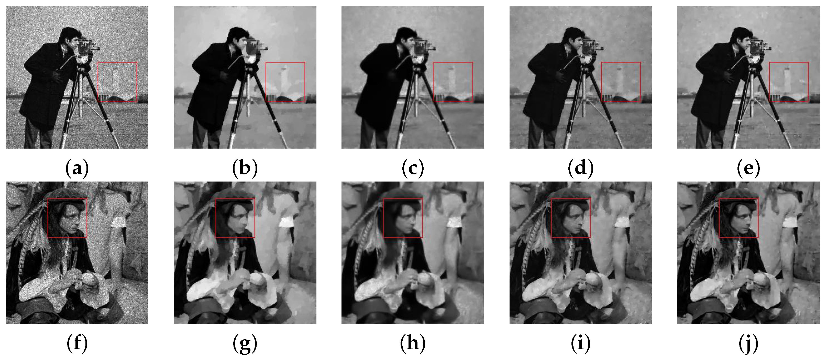
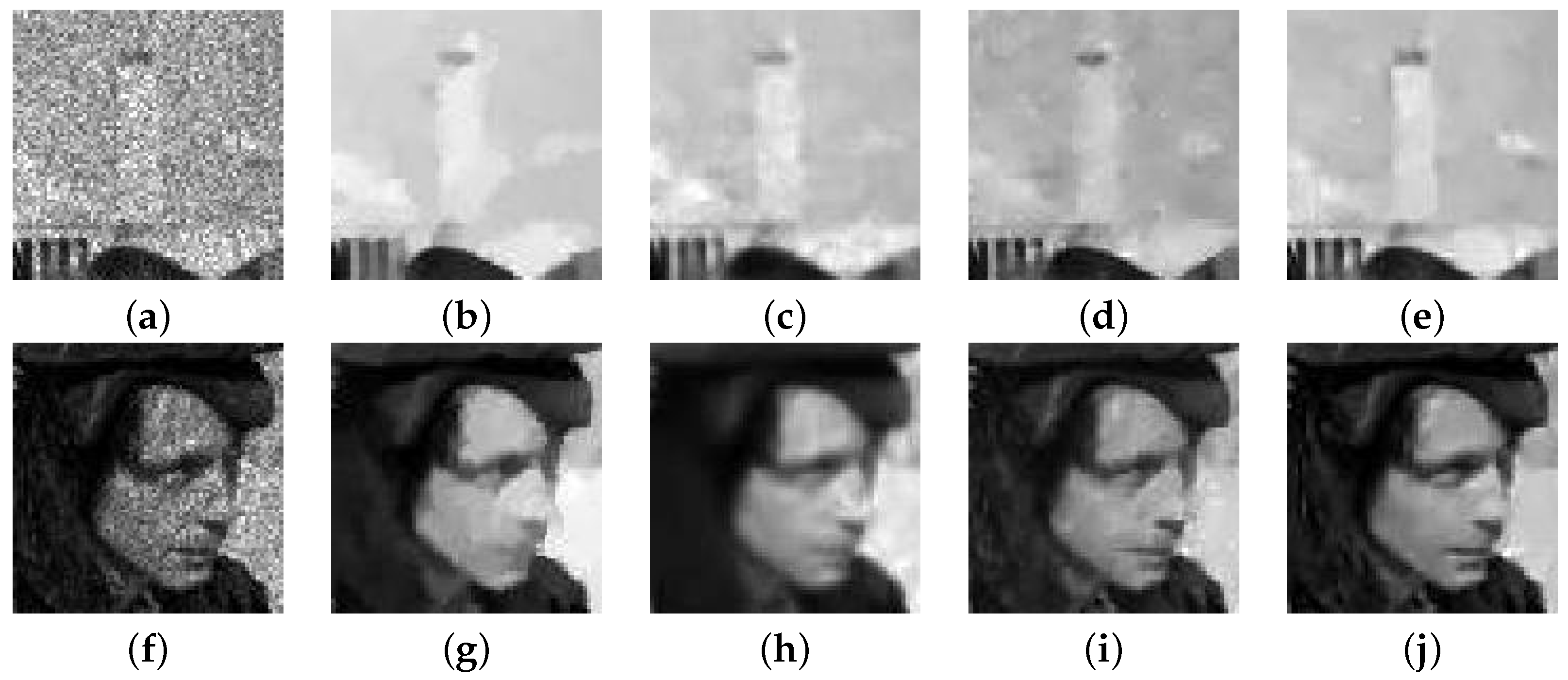
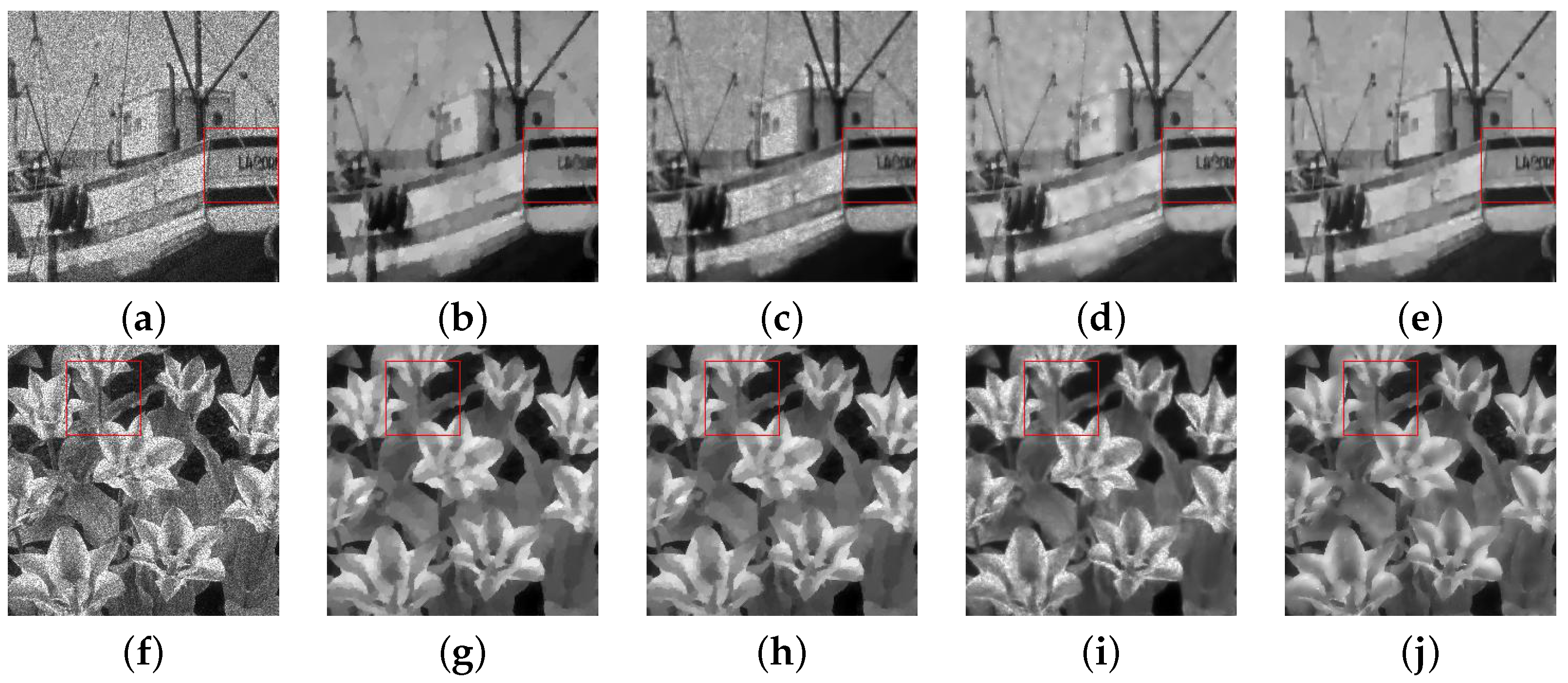
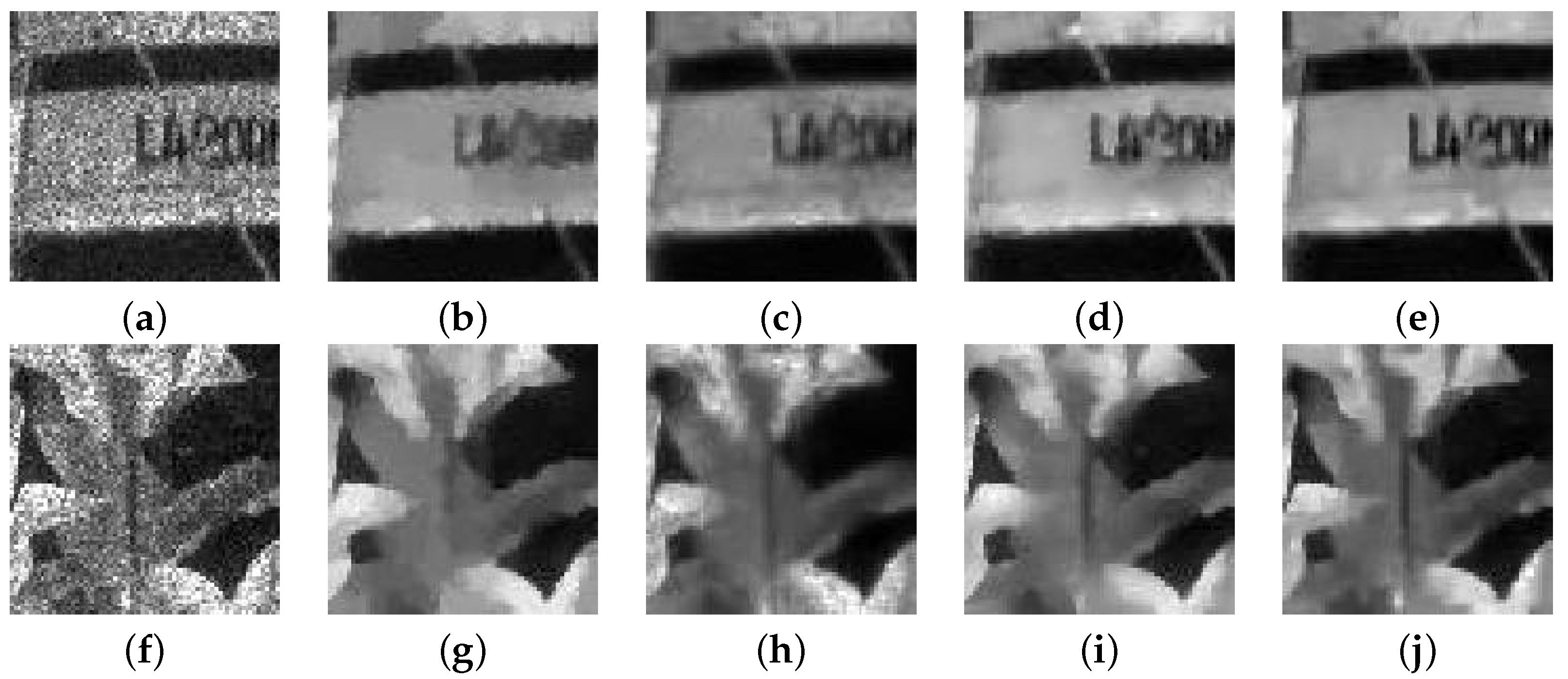
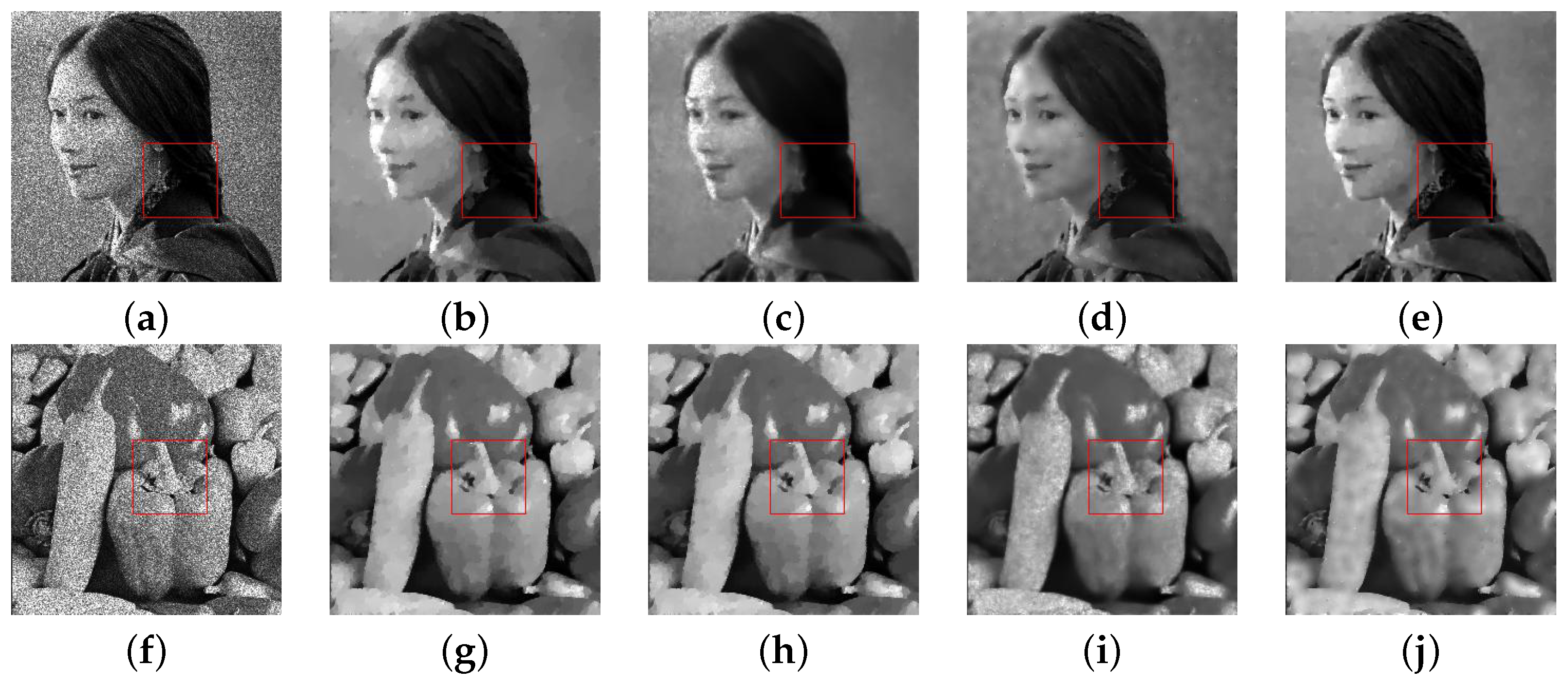
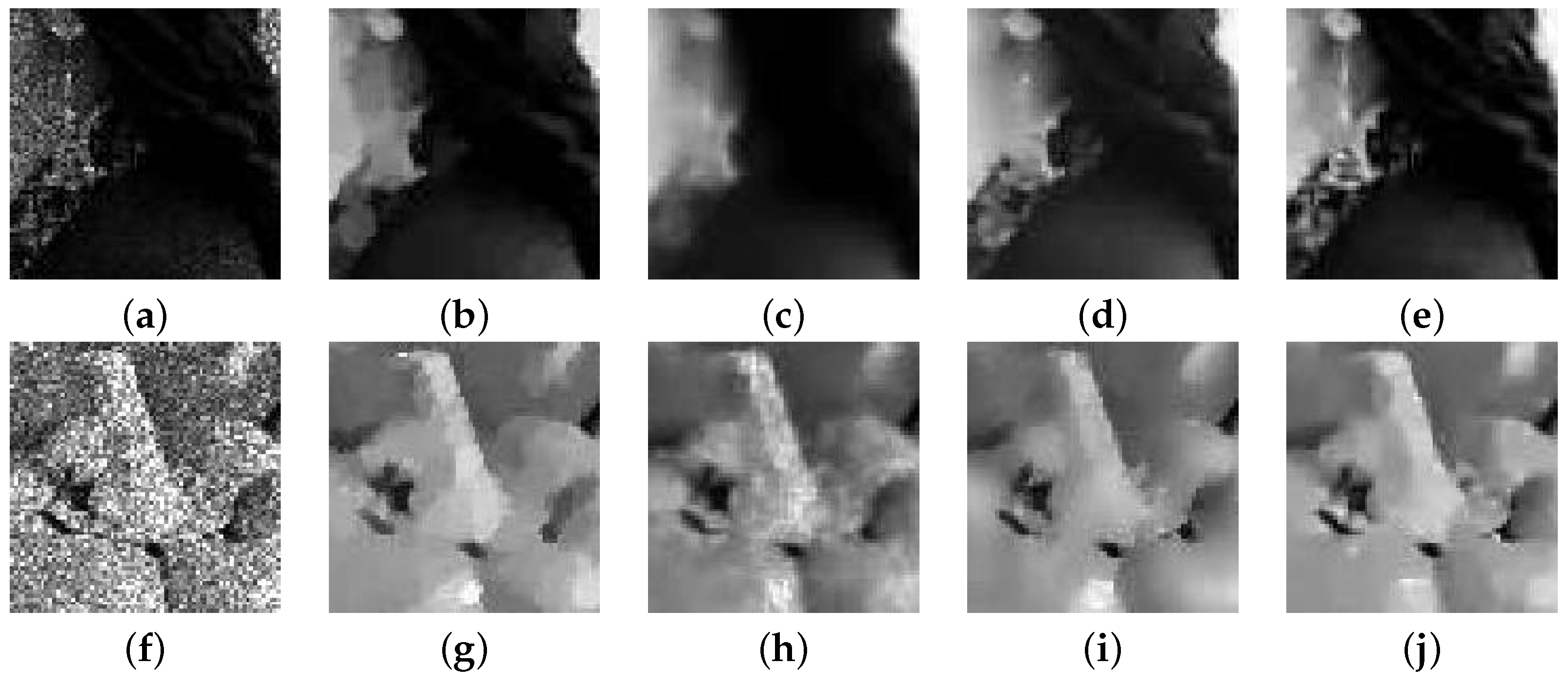
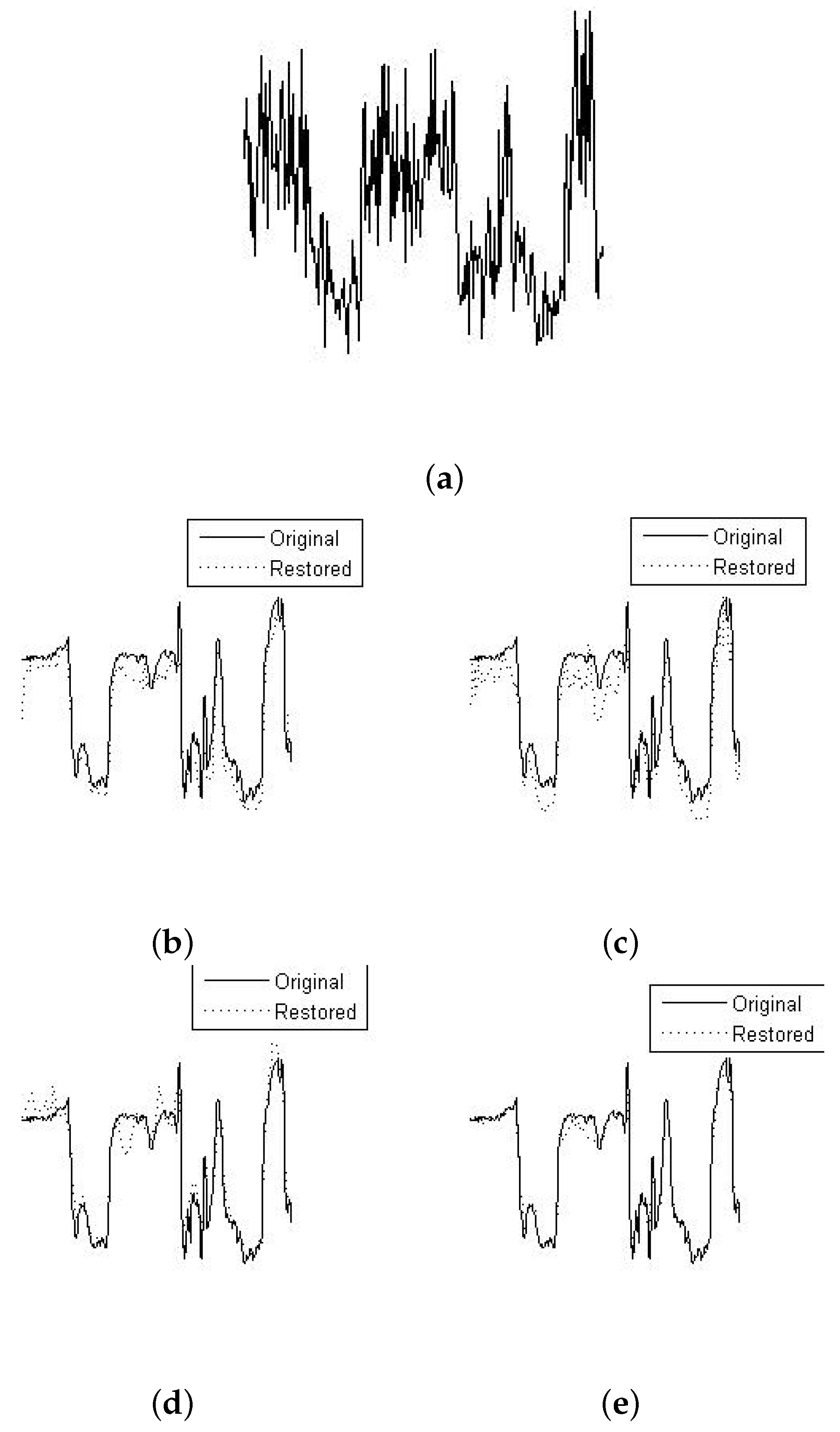
4.2. Experimental Results

In this section, we conducted some experiments to verify the good performance of the proposed algorithm. Firstly, we gave the denoising results of the different methods a noise level of $L=30$ in Figure 3. Figure 3 shows that our method is more competitive in both visual effect and quantitative analysis. We selected the region of the images (the marked red box area in Figure 3) to enlarge to better observe the recovered image. As seen in Figure 3 and Figure 4, our method provides superior recovery for the structure of the restored image. Next, in Figure 5 and Figure 6, the recovery images of “Boats” and “Tulips” are shown for four different methods at a noise level of $L=20$. The other compared methods produce staircase artifacts and lose a lot of detail, while our method successfully overcomes the above shortcomings. Finally, under the noise level $L=10$, the recovered images of “Lin” and “Peppers” by the different methods are shown in Figure 7 and Figure 8. As can be seen in the figures, our method has a great advantage in restoring sharp edges, such as the earrings of “Lin” and the terriers of “Peppers”. Compared with the two models, M-TGV and our method have better performance in restoring detail information and texture structure. Compared with the M-TGV method, our method can restore more details and textures.

Figure 3. Recovery results of four algorithms on different images with the noise at $L=30$: (a) Degraded. (b) CONVEX. (c) OGSTVD. (d) M-TGV. (e) NHOGSHL. (f) Degraded. (g) CONVEX. (h) OGSTVD. (i) M-TGV. (j) NHOGSHL.

Figure 4. Zoomed-in region of Figure 3: (a) Degraded. (b) CONVEX. (c) OGSTVD. (d) M-TGV. (e) NHOGSHL. (f) Degraded. (g) CONVEX. (h) OGSTVD. (i) M-TGV. (j) NHOGSHL.

Figure 5. Recovery results of four algorithms on different images with the noise at $L=20$: (a) Degraded. (b) CONVEX. (c) OGSTVD. (d) M-TGV. (e) NHOGSHL. (f) Degraded. (g) CONVEX. (h) OGSTVD. (i) M-TGV. (j) NHOGSHL.

Figure 6. Zoomed-in region of Figure 5: (a) Degraded. (b) CONVEX. (c) OGSTVD. (d) M-TGV. (e) NHOGSHL. (f) Degraded. (g) CONVEX. (h) OGSTVD. (i) M-TGV. (j) NHOGSHL.

Figure 7. Recovery results of four algorithms on different images with the noise at $L=10$: (a) Degraded. (b) CONVEX. (c) OGSTVD. (d) M-TGV. (e) NHOGSHL. (f) Degraded. (g) CONVEX. (h) OGSTVD. (i) M-TGV. (j) NHOGSHL.

Figure 8. Zoomed-in region of Figure 7: (a) Degraded. (b) CONVEX. (c) OGSTVD. (d) M-TGV. (e) NHOGSHL. (f) Degraded. (g) CONVEX. (h) OGSTVD. (i) M-TGV. (j) NHOGSHL.

To clearly highlight the competitiveness of our method, Figure 9 plots the fifth column of the zoomed “Boats” image under the noise level $L=20$. From the fitting results shown in Figure 9, our method can obtain much better fitting results than the other three methods.

Figure 9. Slice of Boats (the 5th column) and their corresponding denoising results under the noise level $L=20$: (a) Noise image. (b) CONVEX. (c) OGSTVD. (d) M-TGV. (e) NHOGSHL.

Table 1, Table 2 and Table 3 summarize all the PSNRs and SSIMs of the different methods under the different noise levels. From the results in the tables, it is obvious that our method has a higher PSNR and SSIM. These also demonstrate the effectiveness of our method in terms of visual effect and quantitative analysis.

Table 1. Summary of the results of PSNR values and SSIM values restored by different algorithms under the noise level of $L=30$.

Level	Image	CONVEX [28]	OGSTVD [9]	M-TGV [12]	NHOGSHL
		PSNR/SSIM	PSNR/SSIM	PSNR/SSIM	PSNR/SSIM
L = 30	Tulips	25.23/0.7615	25.39/0.7609	27.14/0.8312	27.29/0.8344
	Man	26.19/0.7527	26.08/0.7288	28.39/0.8326	29.04/0.8583
	Camera	25.91/0.7958	26.75/0.7930	29.06/0.8260	29.17/0.8453
	Boats	26.74/0.7603	27.56/0.7869	27.87/0.7926	29.46/0.8372
	Lin	30.88/0.8814	29.93/0.8468	32.47/0.8970	32.61/0.9194
	Peppers	27.01/0.7922	27.40/0.7949	28.99/0.8186	29.56/0.8377

Table 2. Summary of the results of PSNR values and SSIM values restored by different algorithms under the noise level of $L=20$.

Level	Image	CONVEX [28]	OGSTVD [9]	M-TGV [12]	NHOGSHL
		PSNR/SSIM	PSNR/SSIM	PSNR/SSIM	PSNR/SSIM
L = 20	Tulips	24.46/0.7310	24.89/0.7447	25.96/0.7822	26.04/0.7971
	Man	25.63/0.7338	25.88/0.7211	27.07/0.7826	27.90/0.8212
	Camera	25.58/0.7870	26.16/0.7274	27.84/0.8113	28.13/0.8294
	Boats	26.06/0.7434	26.77/0.7350	26.78/0.7623	28.35/0.8122
	Lin	29.03/0.8696	29.39/0.8229	31.39/0.8983	31.82/0.9164
	Peppers	26.28/0.7773	26.69/0.7474	27.90/0.8012	28.78/0.8220

Table 3. Summary of the results of PSNR values and SSIM values restored by different algorithms under the noise level of $L=10$.

Level	Image	CONVEX [28]	OGSTVD [9]	M-TGV [12]	NHOGSHL
		PSNR/SSIM	PSNR/SSIM	PSNR/SSIM	PSNR/SSIM
$L=10$	Tulips	22.85/0.6842	23.52/0.6845	24.38/0.7165	24.51/0.7466
	Man	24.34/0.6968	24.48/0.6590	25.65/0.7280	26.46/0.7787
	Camera	23.78/0.7564	23.91/0.7214	26.30/0.7697	26.80/0.7986
	Boats	23.91/0.6858	25.28/0.6817	25.05/0.6966	26.57/0.7553
	Lin	26.67/0.8451	27.70/0.7851	29.50/0.8555	29.93/0.8835
	Peppers	24.25/0.7401	25.22/0.7090	26.41/0.7650	27.03/0.7804

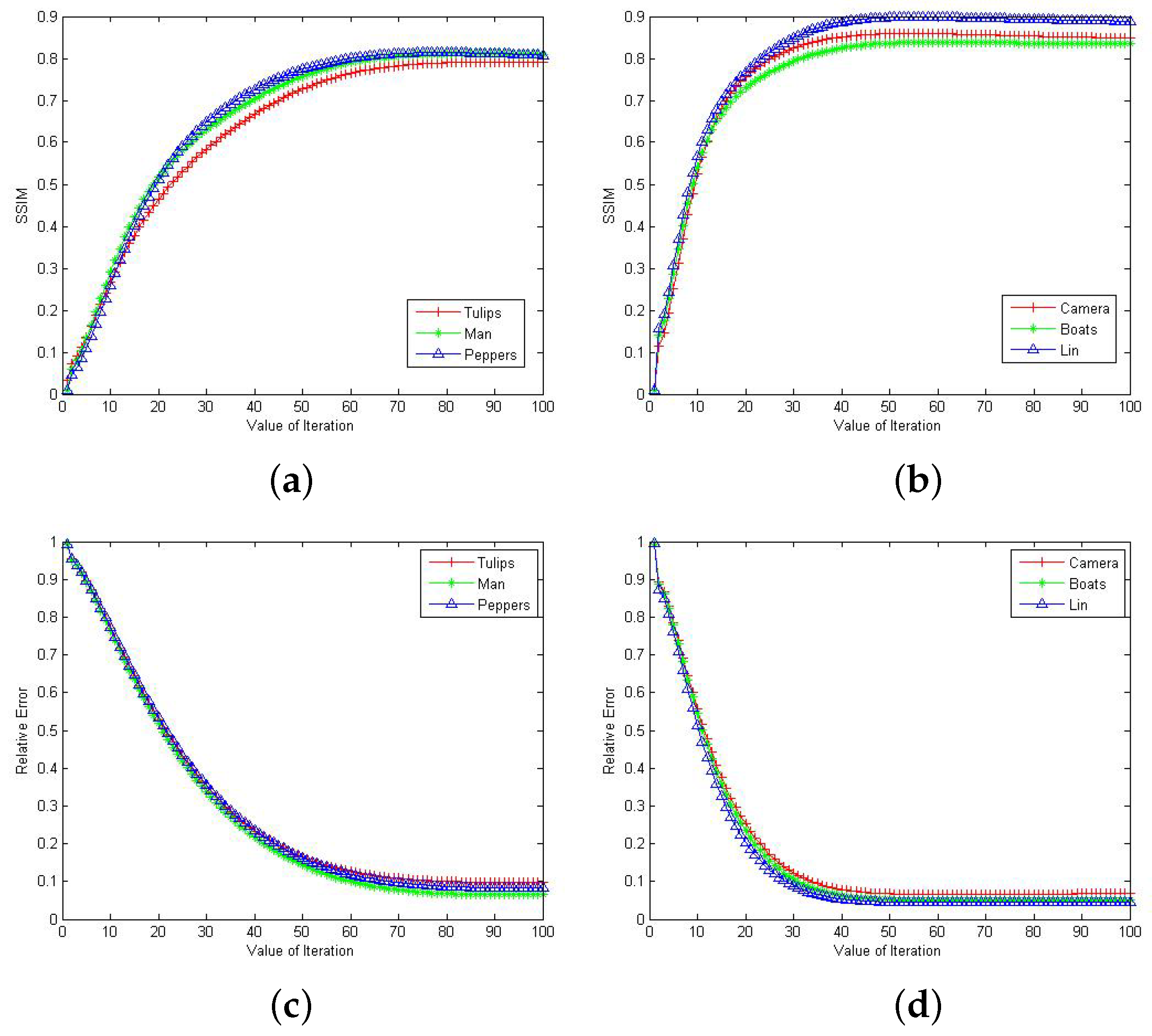
4.3. Convergence Analysis

In this section, we verify the convergence of our method. We plot the curves of SSIM and RelErr values of the restored images versus the iterations under different noise levels in Figure 10. As seen in Figure 10, the curves of relative error are stable as the number of iterations rises.

Figure 10. The SSIM and the ReErr values versus iteration in our model for different images with different noise levels: (a) $L=20$. (b) $L=30$. (c) $L=20$. (d) $L=30$.

5. Conclusions

This paper presents a new nonconvex regularization model for multiplicative noise removal. The new model employs non-convex ${\ell }_p$ norm regularization and OGSHL regularization as a hybrid regularizer. An efficient alternating method is proposed based on an MM algorithm and the iteratively reweighted algorithm to solve the NHOGSHL model under the framework of ADMM. Numerical experiments demonstrate that the NHOGSHL model is competitive against the compared methods. In future work, we hope to extend this method to deal with problems related to removed mixed noises.

References

- Li, F.; Ng, M.K.; Shen, C.M. Multiplicative noise removal with spatially varying regularization parameters. Siam J. Imaging Sci. 2010, 3, 1–20. [Google Scholar] [CrossRef]
- Shi, B.L.; Huang, L.H.; Pang, Z.F. Fast algorithm for multiplicative noise removal. J. Vis. Commun. Image Represent. 2012, 23, 126–133. [Google Scholar] [CrossRef]
- Rudin, L.; Lions, P.L.; Osher, S. Multiplicative denoising and deblurring: Theory and algorithms. In Geometric Level Set Methods in Imaging, Vision, and Graphics; Springer: Berlin/Heidelberg, Germany, 2003; pp. 103–119. [Google Scholar]
- Aubert, G.; Aujol, J.F. A variational approach to removing multiplicative noise. Siam J. Appl. Math. 2008, 68, 925–946. [Google Scholar] [CrossRef]
- Bioucas-Dias, J.M.; Figueiredo, A.T. Multiplicative noise removal using variable splitting and constrained optimization. IEEE Trans. Image Process. 2010, 19, 1720–1730. [Google Scholar] [CrossRef]
- Huang, Y.M.; Ng, M.K.; Wen, Y.W. A new total variation method for multiplicative noise removal. Siam J. Imaging Sci. 2009, 2, 20–40. [Google Scholar] [CrossRef]
- Shi, J.; Osher, S. A nonlinear inverse scale space method for a convex multiplicative noise model. Siam J. Imaging Sci. 2008, 1, 294–321. [Google Scholar] [CrossRef]
- Steidl, G.; Teuber, T. Removing mulitiplicative noise by Douglas-Rachford splitting method. J. Math. Imaging Vis. 2010, 36, 168–184. [Google Scholar] [CrossRef]
- Liu, J.; Huang, T.Z.; Liu, G.; Wang, S.; Lv, X.G. Total variation with overlapping group sparsity for speckle noise reduction. Neurocomputing 2016, 216, 502–513. [Google Scholar] [CrossRef]
- Liu, P. Hybrid higher-order total variation model for multiplicative noise removal. Iet Image Process. 2020, 14, 862–873. [Google Scholar] [CrossRef]
- Shama, M.G.; Huang, T.Z.; Liu, J.; Wang, S. A convex total generalized variation regularized model for multiplicative noise and blur removal. Appl. Math. Comput. 2016, 276, 109–121. [Google Scholar] [CrossRef]
- Lv, Y.H. Total generalized variation denoising of speckled images using a primal-dual algorithm. J. Appl. Math. Comput. 2020, 62, 489–509. [Google Scholar] [CrossRef]
- Chartrand, R. Exact reconstruction of sparse signals via nonconvex minimization. IEEE Signal Process. Lett. 2007, 14, 707–710. [Google Scholar] [CrossRef]
- Han, Y.; Feng, X.C.; Baciu, G.; Wang, W.W. Nonconvex sparse regularizer based speckle noise removal. Pattern Recognit. 2013, 46, 989–1001. [Google Scholar] [CrossRef]
- Chen, X.J.; Zhou, W.J. Smoothing nonlinear conjugate gradient method for image restoration using nonsmooth nonconvex minimization. Siam J. Imaging Sci. 2010, 3, 765–790. [Google Scholar] [CrossRef]
- Nikolova, M. Analysis of the recovery of edges in images and signals by minimizing nonconvex regularized least-squares. Multiscale Model. Simul. 2005, 4, 960–991. [Google Scholar] [CrossRef]
- Nikolova, M.; Ng, M.K.; Zhang, S.; Ching, W.K. Efficient reconstruction of piecewise constant images using nonsmooth nonconvex mininmization. Siam J. Imaging Sci. 2008, 1, 2–25. [Google Scholar] [CrossRef]
- Krishnan, D.; Fergus, R. Fast image deconvolution using hyper-Laplacian priors. In Proceedings of the Advances in Neural Information Processing Systems 22: 23rd Annual Conference on Neural Information Processing Systems 2009, Vancouver, BC, Canada, 7–10 December 2009; pp. 1033–1041. [Google Scholar]
- Levin, A.; Weiss, Y.; Durand, F.; Freeman, W.T. Understanding and evaluating blind deconvolution algorithms. In Proceedings of the IEEE Conference on Computer Vision and Pattern Recognition 2009, Miami, FL, USA, 20–25 June 2009; pp. 1964–1971. [Google Scholar]
- Fergus, R.; Singh, B.; Hertzmann, A.; Roweis, S.T.; Freeman, W.T. Removing camera shake from a single photograph. ACM Trans. Graphics 2006, 25, 787–794. [Google Scholar] [CrossRef]
- Chang, Y.; Yan, L.; Zhong, S. Hyper-Laplacian regularized unidirectional lowrank tensor recovery for multispectral image denoising. In Proceedings of the IEEE Conference on Computer Vision and Pattern Recognition 2017, Honolulu, HI, USA, 21–26 July 2017; pp. 5901–5909. [Google Scholar]
- Kong, J.; Lu, K.; Jiang, M. A new blind deblurring method via hyper-Laplacian prior. Procedia Comput. Sci. 2017, 107, 789–795. [Google Scholar] [CrossRef]
- Zuo, W.M.; Meng, D.Y.; Zhang, L.; Feng, X.C.; Zhang, D. A generalized iterated shrinkage algorithm for non-convex sparse coding. In Proceedings of the IEEE International Conference on Computer Vision 2013, Sydney, Australia, 3–6 December 2013; pp. 217–224. [Google Scholar]
- Shi, M.Z.; Han, T.T.; Liu, S.Q. Total variation image restoration using hyper-Laplacian prior with overlapping group sparsity. Signal Process. 2016, 126, 65–76. [Google Scholar] [CrossRef]
- Liu, J.; Huang, T.Z.; Selesnick, I.W.; Lv, X.G.; Chen, P.Y. Image restoration using total variation with overlapping group sparsity. Inf. Sci. 2015, 295, 232–246. [Google Scholar] [CrossRef]
- Jon, K.; Sun, Y.; Li, Q.X.; Liu, J.; Wang, X.F.; Zhu, W.S. Image restoration using overlapping group sparsity on hyper-Laplacian prior of image gradient. Neurocomputing 2021, 420, 57–69. [Google Scholar] [CrossRef]
- Candès, E.J.; Wakin, M.B.; Boyd, S.P. Enhancing sparsity by reweighted ℓ1 minimization. J. Fourier Anal. Appl. 2008, 14, 877–905. [Google Scholar] [CrossRef]
- Zhao, X.L.; Wang, F.; Ng, M.K. A new convex optimization model for multiplicative noise and blur removal. Siam J. Imaging Sci. 2014, 7, 456–475. [Google Scholar] [CrossRef]
- Wang, Z.; Bovik, A.C.; Sheikh, H.R.; Simoncelli, E.P. Image quality assessment: From error visibility to structural similarity. IEEE Trans. Image Process. 2004, 13, 600–612. [Google Scholar] [CrossRef] [PubMed]
Disclaimer/Publisher’s Note: The statements, opinions and data contained in all publications are solely those of the individual author(s) and contributor(s) and not of MDPI and/or the editor(s). MDPI and/or the editor(s) disclaim responsibility for any injury to people or property resulting from any ideas, methods, instructions or products referred to in the content. |
© 2023 by the authors. Licensee MDPI, Basel, Switzerland. This article is an open access article distributed under the terms and conditions of the Creative Commons Attribution (CC BY) license (https://creativecommons.org/licenses/by/4.0/).