Numerical Approximations for the Solutions of Fourth Order Time Fractional Evolution Problems Using a Novel Spline Technique

Abstract

Developing mathematical models of fractional order for physical phenomena and constructing numerical solutions for these models are crucial issues in mathematics, physics, and engineering. Higher order temporal fractional evolution problems (EPs) with Caputo’s derivative (CD) are numerically solved using a sextic polynomial spline technique (SPST). These equations are frequently applied in a wide variety of real-world applications, such as strain gradient elasticity, phase separation in binary mixtures, and modelling of thin beams and plates, all of which are key parts of mechanical engineering. The SPST can be used for space discretization, whereas the backward Euler formula can be used for time discretization. For the temporal discretization, the method’s convergence and stability are assessed. To show the accuracy and applicability of the proposed technique, numerical simulations are employed.

1. Introduction

Fractional derivatives (FD) and Fractional integrals (FI) are no longer a novel concept. FDs gain considerable attention, because of its non-local property, in few decades. FDs are the leading tool for description of problems in biology, physics, chemistry and in many other areas. FDs may also be used to describe the memory and heredity features of different materials and processes. Non-integer order derivatives and integrals are demonstrably more effective than classical models for expressing some electrochemical difficulties. Extensions of the wave and diffusion equations are also done with the FD and FI operators. The brief history and detailed analysis of this area are provided by Podlubny [1] and Oldham and Spanier [2].

At the same time, applications of the fourth order differential equations are reported in various real life problems. Floor systems, bridge slabs, aeroplane wings, and window panes, for example, may be modelled as plates with various types of boundary supports which can be governed by 4th-order PDEs.

A higher-order EP with time-fractional CD is examined in this study, as follows:

$$\begin{array}{ccc}\hfill \frac{{\partial }^{\gamma }\chi }{\partial t^{\gamma }}+\eta \frac{{\partial }^4\chi }{\partial s^4}& =& g(s,t),s\in \mathrm{\Lambda }=[0,b],t\in (0,T],\hfill \end{array}$$

(1)

subject to the initial condition (IC)

$$\begin{array}{ccc}\hfill \chi (s,0)& =& v_0\left(s\right),0\le s\le b,\hfill \end{array}$$

and boundary conditions (BCs)

$$\left\{\begin{array}{c}\chi (0,t)=\chi (b,t)=0,\hfill \\ {\chi }_{ss}(0,t)={\chi }_{ss}(b,t)=0,t\in (0,T].\hfill \end{array}\right.$$

(2)

where $\gamma$$(0<\gamma <1)$ denotes the order of the FDs in the Caputo sense, $\eta$ denotes the ratio of the beam’s flexural stiffness to its mass per unit length, and $\chi$ denotes the beam’s transverse displacement. The $g(s,t)$ represents dynamic driving force per unit mass, and $v_0\left(s\right)$ is a continuous function. Berdyshev et al. [3] discussed the existence and uniqueness of the solution of suggested problem as a special case where the authors applied the separation-variables method to prove the unique solvability of direct and inverse problems for a fourth-order mixed type equation, which coincides with suggested problem for $t>0$. As hereditary properties and memory of various materials can be depicted more precisely using the time-fractional derivatives, thus they are useful tool for modeling of different processes.

Several descriptions for the notion of fractional operators, e.g., Caputo, Riemann–Liouville and He’s are presented in the last few years. For any discontinuous problems, it is appropriate to use He’s fractal derivative [4,5,6]. Also, with the help of two-scale transform, the differential equations of fractional order can be converted into classical differential ones, which can be solved easily [7,8]. In this work, the Caputo’s fractional derivative will be used because of its suitability to describe physical systems in the real-world as it guarantees to allow the classical IC and BCs in the mathematical modeling of the system. In this work, for description of fractional derivative, the Caputo derivative is used. The time-fractional CD of order $\gamma$ is defined as:

$$\frac{{\partial }^{\gamma }\chi (s,t)}{\partial t^{\gamma }}=\left\{\begin{array}{c}\frac{1}{\mathrm{\Gamma }(1-\gamma )}{\int }_0^t\frac{\partial \chi (s,p)}{\partial p}\frac{dp}{{(t-p)}^{\gamma }},0<\gamma <1,\hfill \\ \frac{\partial \chi (s,t)}{\partial t},\gamma =1.\hfill \end{array}\right.$$

(3)

When $\gamma =1$, Equation (1) provides 4th-order PDE

$$\begin{array}{ccc}\hfill \frac{\partial \chi }{\partial t}+\eta \frac{{\partial }^4\chi }{\partial s^4}& =& g(s,t),s\in \mathrm{\Lambda }=[0,b],t\in (0,T].\hfill \end{array}$$

(4)

The analytical results of many FDEs cannot be obtained using the existing solutions techniques. Therefore, various numerical techniques have been proposed for the approximate solutions of fractional order differential equations.

A numerical technique for solving 4th-order integro PDE with a weakly singular kernel developed by Yang et al. [9]. Liu et al. [10] constructed a computational scheme using the mixed finite element scheme to obtain numerical solution of fractional order fourth-order differential equation. Khan et al. [11] utilized variational iteration technique to obtain the numerical solution of FDEs of order four. Moghaddam et al. [12] presented a integro quadratic spline scheme to obtain the approximate solution for the class of fractional order problems. Roul et al. [13] constructed a collocation approach for fractional order diffusion equation. They used $L1$ scheme for the time-discretization, whereas the space discretization was observed using sextic B-spline. Abdeljawad et al. [14] proposed some fixed point results to determine the numerical solutions of fractional differential equations. El-Sayed et al. [15] introduced a new numerical approach based on Jacobi polynomials for multi term variable order FDEs.

Fractional Bagely-Torvik equation solved numerically using a non-polynomial spline technique [16]. Pedas and Vikerpuur [17] discussed the spline collocation method for multi-term fractional integro-differential equations with weakly singular kernels. Youssri [18] constructed orthonormal ultraspherical operational matrix algorithm for fractal-fractional Riccati equation via generalized Caputo fractional derivative. Cardone et al. [19] discussed the Nordsieck GLM collocation methods for ordinary differential equations, and on two-step spline collocation methods for fractional differential equations. A predictor-corrector method introduced for the approximate solutions of uncertain FDEs [20]. The fractional Drinfeld-Sokolov-Wilson equation was investigated using a novel numerical computational method [21]. Approximate solution of the fractional stochastic Tricomi-type equation was investigated using a finite difference scheme with Caputo’s derivative [22]. Legendre wavelet method was implemented successfully for the numerical computations of the solution of a system of fractional order Volterra integral-differential equations [23]. It is well-known that there is a wide range of effective and robust tools for the solutions of fractional differential equations, namely, the Chun-Hui He’s iteration method [24], the Fourier spectral method [25], reproducing kernel method [26], the variational method [27], spline method [28], the He-Laplace method [29], Integral balance methods [30], lower and upper solutions method [31], and Li-He method [32]. Although existing tools are useful for solving these problems, the expansion of applications and the introduction of new-found and generalized forms for existing equations can be considered the best reason to explore new, useful, and more effective tools.

The main goal of this work to achieve the numerical solution of 4th-order time-fractional boundary value problem using a spline technique based on sextic polynomials. In order to solve PDEs, a sextic spline is broadly applied. If the numerical solutions of FPDE are required at several knots within a particular region, spline solutions ensure that the information about spline interpolation between mesh points is provided. The proposed method uses the piecewise defined spline functions over the spatial domain and it offers a continuous differentiable approximation to the solution with great accuracy but despite any insight into generalizations are not guaranteed. Also, its straightforward applicability provides a reliable base for utilizing it in the framework of numerical solutions for partial differential equations.

The following is how the paper is structured: Section 2 presents materials and methods including some preliminary, a brief overview of SPST, the consistency relations (CR) between the values of the spline and its derivatives at knots are derived using derivative continuities at knots, temporal discretization of the given problem, the first order backward Euler technique, the topic of temporal discretization’s stability and error analysis and the SPST for spatial discretization. In Section 3, numerical results are presented to demonstrate the method’s efficacy. The closing remarks are noted in Section 4.

2. Materials and Methods

2.1. Preliminary Results

Definition 1.

The inner product and norm of $L^2\left(\mathrm{\Lambda }\right)$ can be defined as follows:

$$\begin{array}{c}\hfill ⟨\varphi ,\psi ⟩={\int }_{\mathrm{\Lambda }}vwds,{∥\psi ∥}_0={⟨\psi ,\psi ⟩}^{\frac{1}{2}},\end{array}$$

where the $L^2\left(\mathrm{\Lambda }\right)$ is the space of measurable functions whose square is Lebesgue integrable in Λ.

In order to verify the accuracy of the proposed method, the maximum norm errors and $L_2$ norm errors between numerical and exact solutions are given by the following definitions:

Definition 2.

The maximum norm error is defined as follows:

$$\parallel e_K{\parallel }_{\infty }=\underset{0\le i\le N}{max}|\chi (s_i,t_K)-{\mathbf{Ø}}_{\mathbf{i}}^{\mathbf{K}}|.$$

Definition 3.

The $L_2$ norm error is defined as follows:

$$\parallel e_K{\parallel }_2=\frac{1}{N}{\left(\sum _{i=0}^N{|\chi (s_i,t_K)-{\mathbf{Ø}}_{\mathbf{i}}^{\mathbf{K}}|}^2\right)}^{\frac{1}{2}}.$$

2.2. Sextic Polynomial Spline Functions

The interval $[0,b]$ is uniformly partitioned into the subintervals $[s_{j-1},s_j]$ defined on the grid points $s_j=j\rho$$(j=0,1,\dots ,k,\rho =\frac{b}{k},k>0)$ . It is assumed that the function $u\left(s\right)$ is a differentiable function on given domain $[0,b]$ which is to be approximated by a SPS, $P\left(s\right)$. Each SPS segment $T_j\left(s\right)$ is considered, as:

$$T_j\left(s\right)=a_j{(s-s_j)}^6+b_j{(s-s_j)}^5+c_j{(s-s_j)}^4+d_j{(s-s_j)}^3+e_j{(s-s_j)}^2+g_j(s-s_j)+v_j,$$

(5)

$j=0,1,\dots ,k,$ along with the requirement that

• $T_j\left(s\right)\in C^5[0,b],$
• $P\left(s\right)=T_j\left(s\right),$    $\forall s\in [s_j,s_{j+1}]$, $j=0,1,\dots ,k-1$.

To determine the CR between the values of a spline and its derivatives at knots, the following relations must exist

$$\begin{array}{cc}T{}_j\left(s_j\right)=P_j,\hfill & T_j\left(s_{j+1}\right)=P_{j+1},T_j^{\left(1\right)}\left(s_j\right)=Z_j,\hfill \\ T{}_j^{\left(2\right)}\left(s_j\right)=S_j,\hfill & T_j^{\left(2\right)}\left(s_{j+1}\right)=S_{j+1},T_j^{\left(4\right)}\left(s_j\right)=G_j,\hfill \\ T{}_j^{\left(4\right)}\left(s_{j+1}\right)=G_{j+1}.\hfill \end{array}$$

It should be noted that the spline P can be stated in terms of $P_j$’s and any three derivatives at the subinterval precincts. The coefficients introduced in Equation (5) to express the spline in positions of $P_j$’s, $S_j$’s, $Z_j$’s, and $G_j$’s are determined as follows:

$$\begin{array}{cc}\hfill a_j& =\frac{1}{3{\rho }^6}(P_{j+1}-P_j)-\frac{1}{3{\rho }^5}{Z}_j-\frac{1}{18{\rho }^4}(S_{j+1}+2S_j)+\frac{1}{1080{\rho }^2}(7G_{j+1}+8G_j),\hfill \\ \hfill b_j& =-\frac{1}{{\rho }^5}(P_{j+1}-P_j)+\frac{1}{{\rho }^4}{Z}_j+\frac{1}{6{\rho }^3}(S_{j+1}+2S_j)-\frac{1}{360\rho }(4G_{j+1}+11G_j),\hfill \\ \hfill c_j& =\frac{1}{24}{G}_j,\hfill \\ \hfill d_j& =\frac{5}{3{\rho }^3}(P_{j+1}-P_j)-\frac{5}{3{\rho }^2}{Z}_j-\frac{1}{18\rho }(2S_{j+1}+13S_j)+\frac{\rho }{216}(G_{j+1}-4G_j),\hfill \\ \hfill e_j& =\frac{1}{2}{S}_j,\hfill \\ \hfill g_j& =Z_j,\hfill \\ \hfill v_j& =P_j.\hfill \end{array}$$

At the knots, the 1st, 3rd, and 5th derivative continuities are applied, i.e., $T_j^{\left(\xi \right)}\left(s_j\right)=T_{j-1}^{\left(\xi \right)}\left(s_j\right),$ $\xi =1,3$ and 5, yield the following relations:

$$Z_j+Z_{j-1}=\frac{2}{\rho }(P_j-P_{j-1})+\frac{\rho }{6}(S_j-S_{j-1})-\frac{{\rho }^3}{360}(G_j-G_{j-1}),$$

(6)

$$Z_j+Z_{j-1}=\frac{1}{\rho }(P_{j+1}-P_{j-1})-\frac{\rho }{30}(2S_{j+1}+21S_j+7S_{j-1})+\frac{{\rho }^3}{360}(G_{j+1}-9G_j+2G_{j-1}),$$

(7)

$$Z_j+Z_{j-1}=\frac{1}{\rho }(P_{j+1}-P_{j-1})-\frac{\rho }{6}(S_{j+1}+3S_j+2S_{j-1})+\frac{{\rho }^3}{360}(4G_{j+1}+21G_j+5G_{j-1}),$$

(8)

From Equations (6) and (7), we get

$$P_{j+1}-2P_j+P_{j-1}=\frac{{\rho }^2}{15}(S_{j+1}+13S_j+S_{j-1})-\frac{{\rho }^4}{360}(G_{j+1}-8G_j+G_{j-1}).$$

(9)

Equations (6) and (8) yield

$$P_{j+1}-2P_j+P_{j-1}=\frac{{\rho }^2}{6}(S_{j+1}+4S_j+S_{j-1})-\frac{{\rho }^4}{180}(2G_{j+1}+11G_j+2G_{j-1}).$$

(10)

Using Equations (9) and (10), the following relations are obtained

$${\rho }^2{S}_j=P_{j+1}-2P_j+P_{j-1}-\frac{{\rho }^4}{360}(G_{j+1}+28G_j+G_{j-1}),$$

(11)

$${\rho }^4{G}_j=20(P_{j+1}-2P_j+P_{j-1})-\frac{2{\rho }^2}{3}(S_{j+1}+28S_j+S_{j-1}).$$

(12)

Eliminating $S_i$, $i=j-1,j,j+1$, from Equation (9) using Equation (11) to obtain the following CR in positions of the 4th-order derivative of $G_j$ and $P_j$, as:

$$\begin{array}{c}{P}_{j+2}-4P_{j+1}+6P_j-4P_{j-1}+P_{j-2}=\frac{{\rho }^4}{360}(G_{j+2}+56G_{j+1}+246G_j+56G_{j-1}+G_{j-2}),\hfill \\ \hfill j=2,3,\dots ,k-2.\end{array}$$

(13)

In the $(k-1)$ unknowns, the system (13) generates $(k-3)$ linear algebraic equations. Two further equations (end conditions) are required for $(P_j,j=1,2,\dots ,k-1)$. Taylor series and the technique of undetermined coefficients can be used to derive the two end conditions. Following two end equations are used for unique solution

$$-2P_0+5P_1-4P_2+P_3=-{\rho }^2{S}_0+\frac{{\rho }^4}{360}(28G_0+245G_1+56G_2+G_3),$$

(14)

and

$$P_{k-3}-4P_{k-2}+5P_{k-1}-2P_k=-{\rho }^2{S}_k+\frac{{\rho }^4}{360}(G_{k-3}+56G_{k-2}+245G_{k-1}+28G_k).$$

(15)

An alternative derivation of Equation (13) is given in Appendix A.

2.3. Temporal Discretization

In this section, we discretize the Caputo time-fractional derivative using the Backward Euler scheme. Let us consider $t_n=n\mathrm{\Delta }t$, $n=0,1,\dots ,K$, where $\mathrm{\Delta }t=\frac{T}{K}$ is called the time step size. The Caputo FD at time $t=t_{n+1}$, can be taken as:   

$$\begin{array}{cc}\hfill {\int }_0^{t_{n+1}}\frac{\partial \chi (s,\psi )}{\partial \psi }{(t_{n+1}-\psi )}^{-\gamma }d\psi =& \sum _{i=0}^n{\int }_{t_i}^{t_{i+1}}\frac{\partial \chi (s,\psi )}{\partial \psi }{(t_{n+1}-\psi )}^{-\gamma }d\psi \hfill \\ \hfill =& \sum _{i=0}^n\frac{\chi (s,t_{i+1})-\chi (s,t_i)}{\mathrm{\Delta }t}{\int }_{t_i}^{t_{i+1}}{(t_{n+1}-\psi )}^{-\gamma }d\psi +l_{\mathrm{\Delta }t}^{n+1}\hfill \\ \hfill =& \sum _{i=0}^n\frac{\chi (s,t_{i+1})-\chi (s,t_i)}{\mathrm{\Delta }t}{\int }_{t_{n-i}}^{t_{n+1-i}}{\sigma }^{-\gamma }d\sigma +l_{\mathrm{\Delta }t}^{n+1}\hfill \\ \hfill =& \sum _{i=0}^n\frac{\chi (s,t_{n-i+1})-\chi (s,t_{n-i})}{\mathrm{\Delta }t}{\int }_{t_i}^{t_{1+i}}{\sigma }^{-\gamma }d\sigma +l_{\mathrm{\Delta }t}^{n+1}\hfill \\ \hfill =& \frac{1}{1-\gamma }\sum _{i=0}^n\frac{\chi (s,t_{n-i+1})-\chi (s,t_{n-i})}{\mathrm{\Delta }{t}^{\gamma }}({(i+1)}^{1-\gamma }-i^{1-\gamma })\hfill \\ \hfill & +l_{\mathrm{\Delta }t}^{n+1}\hfill \\ \hfill =& \frac{1}{1-\gamma }\sum _{i=0}^n{q}_i\frac{\chi (s,t_{n-i+1})-\chi (s,t_{n-i})}{\mathrm{\Delta }{t}^{\gamma }}+l_{\mathrm{\Delta }t}^{n+1},\hfill \end{array}$$

(16)

where $q_i={(i+1)}^{1-\gamma }-i^{1-\gamma }$ and $\sigma =(t_{n+1}-\psi )$. From definition of CTFD, we have

$$\frac{{\partial }^{\gamma }\chi (s,t_{n+1})}{\partial t^{\gamma }}=\frac{1}{\mathrm{\Gamma }(2-\gamma )}\sum _{i=0}^n{q}_i\frac{\chi (s,t_{n-i+1})-\chi (s,t_{n-i})}{\mathrm{\Delta }{t}^{\gamma }}+l_{\mathrm{\Delta }t}^{n+1}.$$

(17)

Define the semi-discrete FD operator $V_t^{\gamma }$ as:

$$V_t^{\gamma }\chi (s,t_{n+1}):=\frac{1}{\mathrm{\Gamma }(2-\gamma )}\sum _{i=0}^n{q}_i\frac{\chi (s,t_{n-i+1})-\chi (s,t_{n-i})}{\mathrm{\Delta }{t}^{\gamma }}.$$

Then, Equation (17) can be taken as:

$$\frac{{\partial }^{\gamma }\chi (s,t_{n+1})}{\partial t^{\gamma }}=V_t^{\gamma }\chi (s,t_{n+1})+l_{\mathrm{\Delta }t}^{n+1},$$

(18)

where $l_{\mathrm{\Delta }t}^{n+1}$ is the truncation error (TE) between $\frac{{\partial }^{\gamma }\chi (s,t_{n+1})}{\partial t^{\gamma }}$ and $V_t^{\gamma }\chi (s,t_{n+1})$ in [20]. The scheme (1) using $V_t^{\gamma }\chi (s,t_{n+1})$ may be expressed below as an approximation of time-fractional CD at time point $t=t_{n+1}$,

$$V_t^{\gamma }\chi (s,t_{n+1})+\eta \frac{{\partial }^4\chi (s,t_{n+1})}{\partial s^4}=g(s,t_{n+1}).$$

The given equation yields the following form when using Equation (17)

$$ch{i}^{n+1}\left(s\right)+\mu \eta {\chi }_{ssss}^{n+1}=(1-q_1){\chi }^n\left(s\right)+\sum _{i=1}^{n-1}(q_i-q_{i+1}){\chi }^{n-i}\left(s\right)+q_n{\chi }^0\left(s\right)+\mu g^{n+1}\left(s\right),n=1\left(1\right)K-1,$$

(19)

where ${\chi }^{n+1}\left(s\right)=\chi (s,t_{n+1})$ and $\mu =\mathrm{\Delta }{t}^{\gamma }\mathrm{\Gamma }(2-\gamma )$, with BCs and the following IC

$$\begin{array}{ccc}\hfill {\chi }^0& =& v_0\left(s\right),0\le s\le b.\hfill \end{array}$$

Remark 1.

These are the characteristics of the coefficients $q_i$ in Equation (16)

• $q_i$’s are non-negative when $i=0,1,\dots ,n$
• $1=q_0>q_1>q_2>q_3>\dots >q_n$, $q_n\to 0$ as $n\to \infty$
• ${\sum }_{i=0}^n(q_i-q_{i+1})+q_{n+1}=(1-q_1)+{\sum }_{i=1}^{n-1}(q_i-q_{i+1})+q_n=1$

Also the term $l_{\mathrm{\Delta }t}^{n+1}$ is bounded. i.e.,

$$l_{\mathrm{\Delta }t}^{n+1}\le c\mathrm{\Delta }{t}^{2-\gamma },$$

(20)

where c is a constant that is determined by χ.

To apply this three time level approach, the ${\chi }^0$ and ${\chi }^1$ time levels are required. The scheme (19) can be stated in the following way for $n=1$ as:

$$\begin{array}{ccc}\hfill {\chi }^2\left(s\right)+\mu \eta {\chi }_{ssss}^2& =& (1-q_1){\chi }^1\left(s\right)+q_1{\chi }^0\left(s\right)+\mu g^2\left(s\right).\hfill \end{array}$$

(21)

For $n=0$, the scheme can be written as:

$$\begin{array}{ccc}\hfill {\chi }^1\left(s\right)+\mu \eta {\chi }_{ssss}^1& =& v_0\left(s\right)+\mu g^1\left(s\right).\hfill \end{array}$$

(22)

Also, the Equations (19) and (22), as well as BCs and IC, make up the entire semi-discrete issue of Equation (1). The term $l^{n+1}$ is defined as follows [20]:

$$\begin{array}{c}\hfill l^{n+1}:=\mu \left(\frac{{\partial }^{\gamma }\chi (s,t_{n+1})}{\partial t^{\gamma }}-V_t^{\gamma }\chi (s,t_{n+1})\right).\end{array}$$

(23)

The error term $l^{n+1}$ derives from Equations (18) and (20) and has the following form:

$$\begin{array}{c}\hfill \left|l^{n+1}\right|=\varpi \left|l_{\mathrm{\Delta }t}^{n+1}\right|\le c_{\chi }\mathrm{\Delta }{t}^2,\end{array}$$

(24)

where $\varpi =\mathrm{\Gamma }(2-\gamma )\mathrm{\Delta }{t}^{\gamma }$.

In order to bring the weak representation of the problem, several functional spaces, along with their established norms and inner product (IP), are defined as follows:

$$\begin{array}{c}\hfill P^2\left(\mathrm{\Lambda }\right)=\left\{\psi \in L^2\left(\mathrm{\Lambda }\right),{\psi }_s,{\psi }_{ss}\in L^2\left(\mathrm{\Lambda }\right)\right\},\end{array}$$

$$\begin{array}{c}\hfill P_0^2\left(\mathrm{\Lambda }\right)=\left\{\psi \in P^2\left(\mathrm{\Lambda }\right),\psi {{|}_{\partial \mathrm{\Lambda }}=0,{\psi }_s|}_{\partial \mathrm{\Lambda }}=0\right\},\end{array}$$

$$\begin{array}{c}\hfill P^k\left(\mathrm{\Lambda }\right)=\left\{\psi \in L^2\left(\mathrm{\Lambda }\right),\frac{d^r\psi }{d{s}^r}\in L^2\left(\mathrm{\Lambda }\right),\mathrm{for}\mathrm{all}\mathrm{positive}\mathrm{integer}r\le k\right\},\end{array}$$

where ${\psi }_s=\frac{d\psi }{ds}$ and ${\psi }_{ss}=\frac{d^2\psi }{d{s}^2}$. The IP and norm of $P^2\left(\mathrm{\Lambda }\right)$ can be determined by

$$\begin{array}{c}\hfill {⟨\varphi ,\psi ⟩}_2=⟨\varphi ,\psi ⟩+⟨{\varphi }_s,{\psi }_s⟩+⟨{\varphi }_{ss},{\psi }_{ss}⟩,{∥\psi ∥}_2={⟨\psi ,\psi ⟩}_2^{\frac{1}{2}}.\end{array}$$

The norm $∥.∥$ of the space $P^k\left(\mathrm{\Lambda }\right)$ is defined as:

$$\begin{array}{c}\hfill {∥\psi ∥}_k={\left(\sum _{r=0}^k{∥\frac{d^r\psi }{d{s}^r}∥}_0^2\right)}^{\frac{1}{2}}.\end{array}$$

It is preferable to define ${\parallel .\parallel }_2$ by instead of using the above usual $P^2$-norm

$$\begin{array}{c}\hfill {\parallel \psi \parallel }_2={\left({\parallel \psi \parallel }_0^2+\mu \eta {∥{\psi }_{ss}∥}_0^2\right)}^{1/2}.\end{array}$$

(25)

The following required variational weak version of Equations (19) and (22) is used to investigate the stability and convergence, i.e., finding ${\chi }^{k+1}\in P_0^2\left(\mathrm{\Lambda }\right)$, such that $\forall \psi \in P_0^2\left(\mathrm{\Lambda }\right)$,   

$$\begin{array}{ccc}\hfill & & ⟨{\chi }^{n+1},\psi ⟩+\mu \eta ⟨\frac{{\partial }^4{\chi }^{n+1}}{\partial s^4},\psi ⟩\hfill \\ \hfill & =& \left(1-q_1\right)⟨{\chi }^n,\psi ⟩+\sum _{i=1}^{n-1}\left(q_i-q_{i+1}\right)⟨{\chi }^{n-i},\psi ⟩+q_n⟨{\chi }^0,\psi ⟩+\mu ⟨g^{n+1},\psi ⟩,\hfill \end{array}$$

(26)

and

$$\begin{array}{ccc}\hfill & & ⟨{\chi }^1,\psi ⟩+\mu \eta ⟨\frac{{\partial }^4{\chi }^1}{\partial s^4},\psi ⟩=⟨{\chi }^0,\psi ⟩+\mu ⟨g^1,\psi ⟩.\hfill \end{array}$$

(27)

2.4. The Stability Analysis

The following theorem discusses the semi-discrete problem’s stability analysis.

Theorem 1.

In the sense that it holds for every $\mathrm{\Delta }t>0$, the semi-discrete issue is unconditionally stable

$$\begin{array}{c}\hfill {∥{\chi }^{n+1}∥}_2\le \left({∥{\chi }^0∥}_0+\mu \sum _{i=1}^{n+1}{∥g^i∥}_0\right),n=0,1,\dots ,K-1,\end{array}$$

(28)

where ${\parallel .\parallel }_2$ is defined in Equation (25).

Proof. 

To establish the result, mathematical induction is utilized. When $n=0$ and $\psi ={\chi }^1$ are used in Equation (27), it may be expressed as follows:

$$\begin{array}{ccc}\hfill & & ⟨{\chi }^1,{\chi }^1⟩+\mu \eta ⟨\frac{{\partial }^4{\chi }^1}{\partial s^4},{\chi }^1⟩=⟨{\chi }^0,{\chi }^1⟩+\mu ⟨g^1,{\chi }^1⟩.\hfill \end{array}$$

(29)

The preceding equation becomes the following when by parts integration is used

$$\begin{array}{c}\hfill ⟨{\chi }^1,{\chi }^1⟩+\mu \eta ⟨\frac{{\partial }^2{\chi }^1}{\partial s^2},\frac{{\partial }^2{\chi }^1}{\partial s^2}⟩=⟨{\chi }^0,{\chi }^1⟩+\mu ⟨g^1,{\chi }^1⟩,\end{array}$$

(30)

Because of BCs on $\psi$, all boundary-related contributions have vanished. Using ${∥\psi ∥}_0\le {∥\psi ∥}_2$ and Schwarz inequality, Equation (30) yields

$$\begin{array}{ccc}\hfill {∥{\chi }^1∥}_2^2& \le & {∥{\chi }^0∥}_0{∥{\chi }^1∥}_0+\mu {∥g^1∥}_0{∥{\chi }^1∥}_0\hfill \\ \hfill & \le & {∥{\chi }^0∥}_0{∥{\chi }^1∥}_2+\mu {∥g^1∥}_0{∥{\chi }^1∥}_2\hfill \\ \hfill {∥{\chi }^1∥}_2& \le & \left({∥{\chi }^0∥}_0+\mu {∥g^1∥}_0\right).\hfill \end{array}$$

(31)

Next, suppose that the result holds for $\psi ={\chi }^i$. i.e.,

$$\begin{array}{ccc}\hfill {∥{\chi }^i∥}_2& \le & \left({∥{\chi }^0∥}_0+\mu \sum _{j=1}^i{∥g^j∥}_0\right),i=2,3,\dots ,n.\hfill \end{array}$$

(32)

Let $\psi ={\chi }^{n+1}$ in Equation (26), it can be written as:

$$\begin{array}{ccc}\hfill & & ⟨{\chi }^{n+1},{\chi }^{n+1}⟩+\mu \eta ⟨\frac{{\partial }^4{\chi }^{n+1}}{\partial s^4},{\chi }^{n+1}⟩\hfill \\ \hfill & =& \left(1-q_1\right)⟨{\chi }^n,{\chi }^{n+1}⟩+\sum _{i=1}^{n-1}\left(q_i-q_{i+1}\right)⟨{\chi }^{n-i},{\chi }^{n+1}⟩+q_n⟨{\chi }^0,{\chi }^{n+1}⟩\hfill \\ & & +\mu ⟨g^{n+1},{\chi }^{n+1}⟩.\hfill \end{array}$$

(33)

The preceding equation becomes the following when by parts integration is used

$$\begin{array}{ccc}\hfill & & ⟨{\chi }^{n+1},{\chi }^{n+1}⟩+\mu \eta ⟨\frac{{\partial }^2{\chi }^{n+1}}{\partial s^2},\frac{{\partial }^2{\chi }^{n+1}}{\partial s^2}⟩\hfill \\ \hfill & =& \left(1-q_1\right)⟨{\chi }^n,{\chi }^{n+1}⟩+\sum _{i=1}^{n-1}\left(q_i-q_{i+1}\right)⟨{\chi }^{n-i},{\chi }^{n+1}⟩\hfill \\ \hfill & & +q_n⟨{\chi }^0,{\chi }^{n+1}⟩+\mu ⟨g^{n+1},{\chi }^{n+1}⟩,\hfill \end{array}$$

(34)

Because of BCs on $\psi$, all boundary-related contributions have vanished. Using Schwarz inequality and ${∥\psi ∥}_0\le {∥\psi ∥}_2$, the above equation yields

$$\begin{array}{ccc}\hfill {∥{\chi }^{n+1}∥}_2^2& \le & \left(1-q_1\right){∥{\chi }^n∥}_0{∥{\chi }^{n+1}∥}_0+\sum _{i=1}^{n-1}\left(q_i-q_{i+1}\right){∥{\chi }^{n-i}∥}_0{∥{\chi }^{n+1}∥}_0\hfill \\ \hfill & & +q_n{∥{\chi }^0∥}_0{∥{\chi }^{n+1}∥}_0+\mu {∥g^{n+1}∥}_0{∥{\chi }^{n+1}∥}_0,\hfill \end{array}$$

(35)

or

$$\begin{array}{ccc}\hfill {∥{\chi }^{n+1}∥}_2^2& \le & \left(1-q_1\right){∥{\chi }^n∥}_0{∥{\chi }^{n+1}∥}_2+\sum _{i=1}^{n-1}\left(q_i-q_{i+1}\right){∥{\chi }^{n-i}∥}_0{∥{\chi }^{n+1}∥}_2\hfill \\ \hfill & & +q_n{∥{\chi }^0∥}_0{∥{\chi }^{n+1}∥}_2+\mu {∥g^{n+1}∥}_0{∥{\chi }^{n+1}∥}_2,\hfill \end{array}$$

(36)

or

$$\begin{array}{ccc}\hfill {∥{\chi }^{n+1}∥}_2& \le & \left(1-q_1\right){∥{\chi }^k∥}_0+\sum _{i=1}^{n-1}\left(q_i-q_{i+1}\right){∥{\chi }^{n-i}∥}_0+q_n{∥{\chi }^0∥}_0+\mu {∥g^{n+1}∥}_0.\hfill \end{array}$$

(37)

Using Equation (32), the above equation becomes

$$\begin{array}{ccc}\hfill {∥{\chi }^{n+1}∥}_2& \le & \left[{∥{\chi }^0∥}_0+\mu \sum _{i=1}^n{∥g^i∥}_0\right]\left(\left(1-q_1\right)+\sum _{i=1}^{n-1}\left(q_i-q_{i+1}\right)+q_n\right)\hfill \\ & & +\mu {∥g^{n+1}∥}_0.\hfill \end{array}$$

Using properties of $q_i$, it can be rewritten as:

$$\begin{array}{ccc}\hfill {∥{\chi }^{n+1}∥}_2& \le & \left({∥{\chi }^0∥}_0+\mu \sum _{i=1}^{n+1}{∥g^i∥}_0\right).\hfill \end{array}$$

(38)

   □

Lemma 1.

Consider $\chi (s,t)$ be the exact solution of problem (1) and ${\left\{{\chi }^n\right\}}_{n=0}^K$ be the time-discrete solution of Equations (26) and (27) with IC. Then it holds

$$\begin{array}{ccc}\hfill {∥\chi \left(t_n\right)-{\chi }^n∥}_2& \le & c_{\chi }{q}_{n-1}^{-1}\mathrm{\Delta }{t}^2,n=1,2,\dots ,K.\hfill \end{array}$$

(39)

Proof. 

Let $e^n=\chi (s,t_n)-{\chi }^n\left(s\right)$, for $n=1$, by coalescing Equations (1), (25) and (27), the error equation can be expressed in following form as:

$$\begin{array}{c}\hfill ⟨e^1,\psi ⟩+\mu \eta ⟨\frac{{\partial }^2{e}^1}{\partial s^2},\frac{{\partial }^2\psi }{\partial s^2}⟩=⟨e^0,\psi ⟩+⟨l^1,\psi ⟩,\forall \psi \in P_0^2\left(\mathrm{\Lambda }\right).\end{array}$$

Let $\psi =e^1$, noting $e^0=0$ gives

$$\begin{array}{c}\hfill {∥e^1∥}_2\le {∥l^1∥}_0.\end{array}$$

From above equation and Equation (24),

$$\begin{array}{c}\hfill {∥\chi \left(t_1\right)-{\chi }^1∥}_2\le c_{\chi }{q}_0^{-1}\mathrm{\Delta }{t}^2.\end{array}$$

(40)

Thus, the Equation (39) is completed for $n=1$.

The Equation (39) satisfies for $n=1\left(1\right)r$, i.e.,

$$\begin{array}{c}\hfill {∥\chi \left(t_n\right)-{\chi }^n∥}_2\le c_{\chi }{q}_{n-1}^{-1}\mathrm{\Delta }{t}^2.\end{array}$$

(41)

The Equations (1), (25) and (26) can be used for $n=r+1$, the error equation for all $\psi \in P_0^2\left(\mathrm{\Lambda }\right)$ can be written as:

$$\begin{array}{ccc}\hfill & & ⟨e^{n+1},\psi ⟩+\mu \eta ⟨\frac{{\partial }^2{e}^{n+1}}{\partial s^2},\frac{{\partial }^2\psi }{\partial s^2}⟩\hfill \\ \hfill & =& \left(1-q_1\right)⟨e^n,\psi ⟩+\sum _{i=1}^{n-1}\left(q_i-q_{i+1}\right)⟨e^{n-i},\psi ⟩+q_n⟨e^0,\psi ⟩+⟨l^{n+1},\psi ⟩.\hfill \end{array}$$

Take $\psi =e^{n+1}$, use the induction assumption and the relation $\frac{q_i^{-1}}{q_{i+1}^{-1}}<1$ for all non negative integer i, then above equation becomes

$$\begin{array}{ccc}\hfill {∥e^{n+1}∥}_2& \le & c_{\chi }{q}_n^{-1}\mathrm{\Delta }{t}^2.\hfill \end{array}$$

   □

Using the definition of $q_n$, the following equation may be derived as:

$$\begin{array}{ccc}\hfill \underset{n\to \infty }{lim}\frac{q_{n-1}^{-1}}{n^{\gamma }}& =& \underset{n\to \infty }{lim}\frac{n^{-\gamma }}{n^{1-\gamma }-{(n-1)}^{1-\gamma }}\hfill \\ \hfill & & =\underset{n\to \infty }{lim}\frac{n^{-1}}{1-{(1-\frac{1}{n})}^{1-\gamma }}\hfill \\ \hfill & & =\frac{1}{(1-\gamma )}.\hfill \end{array}$$

The function $\mathrm{\Theta }\left(y\right)$ can be defined as: $\mathrm{\Theta }\left(y\right):=\frac{y^{-\gamma }}{y^{1-\gamma }-{(y-1)}^{1-\gamma }}$. This function is increasing on y for all $y>1$ since ${\mathrm{\Theta }}^{{}^{\prime }}\left(y\right)\ge 0,\forall y>1$. It can be concluded that $1<n\to \infty$, $\frac{q_{n-1}^{-1}}{n^{\gamma }}$ is increasingly tends to $\frac{1}{(1-\gamma )}$. As, $n^{-\gamma }{q}_{n-1}^{-1}=1$ for $n=1$, hence it can written in following form

$$\begin{array}{c}\hfill n^{-\gamma }{q}_{n-1}^{-1}\le \frac{1}{(1-\gamma )},n=1,2,\dots ,K.\end{array}$$

Consequently, for all n such that $n\mathrm{\Delta }t\le T$,

$$\begin{array}{ccc}\hfill {∥\chi \left(t_n\right)-{\chi }^n∥}_2& \le & c_{\chi }{q}_{n-1}^{-1}\mathrm{\Delta }{t}^2\hfill \\ \hfill & =& c_{\chi }{n}^{-\gamma }{q}_{n-1}^{-1}{n}^{\gamma }\mathrm{\Delta }{t}^{2-\gamma +\gamma }\hfill \\ \hfill & \le & c_{\chi }\frac{1}{1-\gamma }{\left(n\mathrm{\Delta }t\right)}^{\gamma }\mathrm{\Delta }{t}^{2-\gamma }\hfill \\ \hfill & \le & c_{\chi ,\gamma }{T}^{\gamma }\mathrm{\Delta }{t}^{2-\gamma }.\hfill \end{array}$$

The above results can be summarized in the following theorem as:

Theorem 2.

Let χ be the exact solution of Equation (1) and ${\left\{{\chi }^n\right\}}_{n=0}^K$ be the time-discrete solution of Equations (26) and (27) with IC ${\chi }^0=v_0\left(s\right),0\le s\le b$, then it holds

$$\begin{array}{ccc}\hfill {∥\chi \left(t_n\right)-{\chi }^n∥}_2& \le & c_{\chi ,\gamma }{T}^{\gamma }\mathrm{\Delta }{t}^{2-\gamma },n=1,2,\dots ,K.\hfill \end{array}$$

(42)

2.5. Space Discretization

Consider the grid points $(s_j,t_n)$ of a uniform mesh with, to discretize the region $[0,b]\times [0,T]$, where $s_j=jh$, $j=0,1,\dots ,k$, and $t_n=n\mathrm{\Delta }t$, $n=0,1,\dots ,K$, $T=K\mathrm{\Delta }t$. The $\mathrm{\Delta }t$ and $\rho$ are the step sizes in the time and space, respectively.

The space discretization of Equation (19) using SPS is carried out as:

$$P_j^{n+1}+\mu \eta G_j^{n+1}=(1-q_1)P_j^n+\sum _{i=1}^{n-1}(q_i-q_{i+1})P_j^{n-i}+q_n{v}_j+\mu g_j^{n+1}.$$

(43)

The operator $\mathrm{\Omega }$ is defined as follows:

$$\mathrm{\Omega }{p}_i=246p_i+56(p_{i-1}+p_{i+1})+(p_{i-2}+p_{i+2}).$$

(44)

Now, Equation (13) can be written as:

$$\mathrm{\Omega }{G}_j=\frac{360}{{\rho }^4}(P_{j-2}-4P_{j-1}+6P_j-4P_{j+1}+P_{j+2}).$$

(45)

Using operator $\mathrm{\Omega }$, the Equation (43) yields,

$$\begin{array}{ccc}\hfill & & \left(P_{j-2}^{n+1}+56P_{j-1}^{n+1}+246P_j^{n+1}+56P_{j+1}^{n+1}+P_{j+2}^{n+1}\right)\hfill \\ \hfill & & +\mu \eta \frac{360}{{\rho }^4}\left(P_{j-2}^{n+1}-4P_{j-1}^{n+1}+6P_j^{n+1}-4P_{j+1}^{n+1}+P_{j+2}^{n+1}\right)\hfill \\ \hfill & =& \left(1-q_1\right)\left(P_{j-2}^n+56P_{j-1}^n+246P_j^n+56P_{j+1}^n+P_{j+2}^n\right)\hfill \\ \hfill & & +\sum _{i=1}^{n-1}\left(q_i-q_{i+1}\right)\left(P_{j-2}^{n-i}+56P_{j-1}^{n-i}+246P_j^{n-i}+56P_{j+1}^{n-i}+P_{j+2}^{n-i}\right)\hfill \\ \hfill & & +q_n\left(v_{j-2}+56v_{j-1}+246v_j+56v_{j+1}+v_{j+2}\right)\hfill \\ \hfill & & +\mu (g_{j-2}^{n+1}+56g_{j-1}^{n+1}+246g_j^{n+1}+56g_{j+1}^{n+1}+g_{j+2}^{n+1}),\hfill \end{array}$$

(46)

$$\begin{array}{ccc}& & n=1,2,\dots ,K-1.\hfill \end{array}$$

(47)

The system gets simpler once, it has been simplified

$$\begin{array}{ccc}\hfill & & \left(\left(1+\mu \eta \frac{360}{{\rho }^4}\right)P_{j-2}^{n+1}+\left(56-4\mu \eta \frac{360}{{\rho }^4}\right)P_{j-1}^{n+1}+\left(246+6\mu \eta \frac{360}{{\rho }^4}\right)P_j^{n+1}\right.\hfill \\ \hfill & & \left.+\left(56-4\mu \eta \frac{360}{{\rho }^4}\right)P_{j+1}^{n+1}+\left(1+\mu \eta \frac{360}{{\rho }^4}\right)P_{j+2}^{n+1}\right)\hfill \\ & =& Q_j,n=1,2,\dots ,K-1,j=2,3,\dots ,k-2,\hfill \end{array}$$

(48)

where,

$$\begin{array}{ccc}\hfill Q_j& =& \left(1-q_1\right)\left(P_{j-2}^n+56P_{j-1}^n+246P_j^n+56P_{j+1}^n+P_{j+2}^n\right)\hfill \\ \hfill & & +\sum _{i=1}^{n-1}\left(q_i-q_{i+1}\right)\left(P_{j-2}^{n-i}+56P_{j-1}^{n-i}+246P_j^{n-i}+56P_{j+1}^{n-i}+q_{j+2}^{n-i}\right)\hfill \\ \hfill & & +q_n\left(v_{j-2}+56v_{j-1}+246q_j+56v_{j+1}+v_{j+2}\right)+\mu (g_{j-2}^{n+1}+56g_{j-1}^{n+1}\hfill \\ \hfill & & +246g_j^{n+1}+56g_{j+1}^{n+1}+g_{j+2}^{n+1}).\hfill \end{array}$$

In the $(k-1)$ unknowns $(P_j^{n+1},j=1,2,\dots ,k-1)$, the system (48) gives $(k-3)$ equations, hence two additional equations are required to obtain a full solution for $P_j^{n+1}$ to be derived.

2.6. Initial State

A five-point approach has been proposed. To use this approach, there is need to find the values of ${\mathbf{P}}^{\mathbf{2}}={[P_1^2,P_2^2,\dots ,P_{k-1}^2]}^T$ and ${\mathbf{P}}^{\mathbf{1}}={[P_1^1,P_2^1,\dots ,P_{k-1}^1]}^T.$ To obtain the value of ${\mathbf{P}}^{\mathbf{2}},$ there is need to find ${\mathbf{P}}^{\mathbf{1}}.$ The value of ${\mathbf{P}}^{\mathbf{1}}$ can be obtained, solving Equation (18) using SPST, as:

$$\begin{array}{ccc}\hfill & & \left(\left(1+\mu \eta \frac{360}{{\rho }^4}\right)P_{j-2}^1+\left(56-4\mu \eta \frac{360}{{\rho }^4}\right)P_{j-1}^1+\left(246+6\mu \eta \frac{360}{{\rho }^4}\right)P_j^1\right.\hfill \\ \hfill & & \left.+\left(56-4\mu \eta \frac{360}{{\rho }^4}\right)P_{j+1}^1+\left(1+\mu \eta \frac{360}{{\rho }^4}\right)P_{j+2}^1\right)\hfill \\ & =& J_j,j=2,3,\dots ,k-2,\hfill \end{array}$$

(49)

where,

$$\begin{array}{ccc}\hfill J_j& =& \left(v_{j-2}+56v_{j-1}+246v_j+56v_{j+1}+v_{j+2}\right)+\mu (g_{j-2}^1+56g_{j-1}^1\hfill \\ \hfill & & +246g_j^1+56g_{j+1}^1+g_{j+2}^1).\hfill \end{array}$$

The Equation (49) provides a system of linear equations $(k-3)\times (k-1)$ with unknown $(P_j^1,j=1,2,\dots ,k-1)$. For a unique solution of this system, we have added two end equations which are given by:

$$\begin{array}{ccc}\hfill & & \left(\left(28-2\mu \eta \frac{360}{{\rho }^4}\right)P_0^1+\left(245+5\mu \eta \frac{360}{{\rho }^4}\right)P_1^1+\left(56-4\mu \eta \frac{360}{{\rho }^4}\right)P_2^1\right.\hfill \\ \hfill & & \left.+\left(1+\mu \eta \frac{360}{{\rho }^4}\right)P_3^1\right)\hfill \\ & =& \left(28v_0+245v_1+56v_2+v_3\right)+\mu (28g_0^1+245g_1^1+56g_2^1+g_3^1),\hfill \end{array}$$

(50)

and

$$\begin{array}{ccc}\hfill & & \left(\left(1+\mu \eta \frac{360}{{\rho }^4}\right)P_{k-3}^1+\left(56-4\mu \eta \frac{360}{{\rho }^4}\right)P_{k-2}^1+\left(245+5\mu \eta \frac{360}{{\rho }^4}\right)P_{k-1}^1\right.\hfill \\ \hfill & & \left.+\left(28-2\mu \eta \frac{360}{{\rho }^4}\right)P_k^1\right)\hfill \\ & =& \left(v_{k-3}+56v_{k-2}+245v_{k-1}+28v_k\right)+\mu (g_{k-3}^1+56g_{k-2}^1+245g_{k-1}^1+28g_k^1).\hfill \end{array}$$

(51)

Let $\mathbf{v}={[v_1,v_2,\dots ,v_{k-1}]}^T$, $\mathbf{g}={[g_1^1,g_2^1,\dots ,g_{k-1}^1]}^T$, $\tilde{\mathbf{v}}={[v_0,0,\dots ,0,v_k]}^T$ and $\tilde{\mathbf{g}}={[g_0^1,0,\dots ,0,g_k^1]}^T$ be the $(k-1)$ dimensional column vectors. The system given by (49)–(51) can be written in matrix form as follows:

$$A{\mathbf{P}}^{\mathbf{1}}=B(\mathbf{v}+\mathbf{g})+C(\tilde{\mathbf{v}}+\tilde{\mathbf{g}}),$$

where,

$$A=\left(\begin{array}{ccc}245+5\mu \eta \frac{360}{{\rho }^4}& 56-4\mu \eta \frac{360}{{\rho }^4}& 1+\mu \eta \frac{360}{{\rho }^4}\\ 56-4\mu \eta \frac{360}{{\rho }^4}& 246+6\mu \eta \frac{360}{{\rho }^4}& 56-4\mu \eta \frac{360}{{\rho }^4}& 1+\mu \eta \frac{360}{{\rho }^4}\\ 1+\mu \eta \frac{360}{{\rho }^4}& 56-4\mu \eta \frac{360}{{\rho }^4}& 246+6\mu \eta \frac{360}{{\rho }^4}& 56-4\mu \eta \frac{360}{{\rho }^4}& 1+\mu \eta \frac{360}{{\rho }^4}\\ & & \ddots \\ & \\ 1+\mu \eta \frac{360}{{\rho }^4}& 56-4\mu \eta \frac{360}{{\rho }^4}& 246+6\mu \eta \frac{360}{{\rho }^4}& 56-4\mu \eta \frac{360}{{\rho }^4}& 1+\mu \eta \frac{360}{{\rho }^4}\\ & 1+\mu \eta \frac{360}{{\rho }^4}& 246+6\mu \eta \frac{360}{{\rho }^4}& 56-4\mu \eta \frac{360}{{\rho }^4}& 56-4\mu \eta \frac{360}{{\rho }^4}\\ & & 1+\mu \eta \frac{360}{{\rho }^4}& 56-4\mu \eta \frac{360}{{\rho }^4}& 245+5\mu \eta \frac{360}{{\rho }^4}\end{array}\right),$$

$$B=\left(\begin{array}{ccc}245& 56& 1\\ 56& 246& 56& 1\\ 1& 56& 246& 56& 1\\ & & & & \ddots \\ & & & \\ & & & 1& 56& 256& 56& 1\\ & & & & 1& 56& 246& 56\\ & & & & & 1& 56& 245\end{array}\right),$$

and

$$C=\left(\begin{array}{ccccc}28& 0& 0& \dots & 0\\ 1& 0& 0& \dots & 0\\ 0& 0& 0& \dots & 0\\ & & \ddots \\ & & \\ 0& 0& 0& \dots & 0\\ 0& & \cdots & 0& 1\\ 0& & \dots & 0& 28\end{array}\right).$$

are $(k-1)\times (k-1)$ matrices.

2.7. Truncation Error for the Spatial Direction

The Equation (46) can be written in the following form, as:

$$\begin{array}{c}\hfill {\rho }^4(360+60{\delta }_s^2+{\delta }_s^4)P_j^{n+1}+360\mu \eta {\delta }_s^4{P}_j^{n+1}=Q_j,\end{array}$$

(52)

where,

$$\begin{array}{ccc}\hfill Q_j& =& {\rho }^4(\left(1-q_1\right)\left(360+60{\delta }_s^2+{\delta }_s^4\right)P_j^{n+1}+\sum _{i=1}^{n-1}\left(q_i-q_{i+1}\right)\left(360+60{\delta }_s^2+{\delta }_s^4\right)P_j^{n-i}\hfill \\ \hfill & & +q_n\left(360+60{\delta }_s^2+{\delta }_s^4\right)v_j+\mu (360+60{\delta }_s^2+{\delta }_s^4)g_j^{n+1}).\hfill \end{array}$$

Expanding Equation (52) with Taylor series in terms of $P(s_j,t_n)$ and its spatial derivatives, the following relations are obtained

$$\begin{array}{ccc}\hfill {\delta }_s^{4}P(s_j,t_n)& =& \left({\rho }^4{D}_s^4+\frac{{\rho }^6}{6}{D}_s^6+\frac{{\rho }^8}{80}{D}_s^8+\frac{17{\rho }^{10}}{3024}{D}_s^{10}+\frac{62{\rho }^{12}}{10!}{D}_s^{12}+\dots \right)P(s_j,t_n),\hfill \\ \hfill {\delta }_s^{2}P(s_j,t_n)& =& \left({\rho }^2{D}_s^2+\frac{2{\rho }^4}{4!}{D}_s^4+\frac{2{\rho }^6}{6!}{D}_s^6+\frac{2{\rho }^8}{8!}{D}_s^8+\dots \right)P(s_j,t_n).\hfill \end{array}$$

(53)

Using Equations (52) and (53), the truncation error is obtained as:

$$\begin{array}{ccc}\hfill T_j& =& {\rho }^4(360+60{\delta }_s^2+{\delta }_s^4)P_j^{n+1}+360\mu \eta {\delta }_s^4{P}_j^{n+1}-{\rho }^4\left(\left(1-q_1\right)\right(360+60{\delta }_s^2+{\delta }_s^4)P_j^{n+1}\hfill \\ \hfill & & +\sum _{i=1}^{n-1}\left(q_i-q_{i+1}\right)\left(360+60{\delta }_s^2+{\delta }_s^4\right)P_j^{n-i}+q_n\left(360+60{\delta }_s^2+{\delta }_s^4\right)v_j+\mu (360+60{\delta }_s^2\hfill \\ \hfill & & +{\delta }_s^4)(D_t^{2-\gamma }+\eta D_s^4)P_j^{n+1}),\hfill \end{array}$$

$$\begin{array}{ccc}\hfill T_j& =& {\rho }^4(360+60\left({\rho }^2{D}_s^2+\frac{2{\rho }^4}{4!}{D}_s^4+\frac{2{\rho }^6}{6!}{D}_s^6+\frac{2{\rho }^8}{8!}{D}_s^8+\dots \right)+({\rho }^4{D}_s^4+\frac{{\rho }^6}{6}{D}_s^6+\frac{{\rho }^8}{80}{D}_s^8\hfill \\ \hfill & & +\frac{17{\rho }^{10}}{3024}{D}_s^{10}+\frac{62{\rho }^{12}}{10!}{D}_s^{12}+\dots \left)\right)P_j^{n+1}+360\mu \eta ({\rho }^4{D}_s^4+\frac{{\rho }^6}{6}{D}_s^6+\frac{{\rho }^8}{80}{D}_s^8+\frac{17{\rho }^{10}}{3024}{D}_s^{10}\hfill \\ \hfill & & +\frac{62{\rho }^{12}}{10!}{D}_s^{12}+\dots )P_j^{n+1}-{\rho }^4((1-q_1)(360+60({\rho }^2{D}_s^2+\frac{2{\rho }^4}{4!}{D}_s^4+\frac{2{\rho }^6}{6!}{D}_s^6\hfill \\ \hfill & & +\frac{2{\rho }^8}{8!}{D}_s^8+\dots )+({\rho }^4{D}_s^4+\frac{{\rho }^6}{6}{D}_s^6+\frac{{\rho }^8}{80}{D}_s^8+\frac{17{\rho }^{10}}{3024}{D}_s^{10}+\frac{62{\rho }^{12}}{10!}{D}_s^{12}+\dots ))P_j^{n+1}\hfill \\ \hfill & & +\sum _{i=1}^{n-1}(q_i-q_{i+1})(360+60({\rho }^2{D}_s^2+\frac{2{\rho }^4}{4!}{D}_s^4+\frac{2{\rho }^6}{6!}{D}_s^6+\frac{2{\rho }^8}{8!}{D}_s^8+\dots )+({\rho }^4{D}_s^4+\frac{{\rho }^6}{6}{D}_s^6\hfill \\ \hfill & & +\frac{{\rho }^8}{80}{D}_s^8+\frac{17{\rho }^{10}}{3024}{D}_s^{10}+\frac{62{\rho }^{12}}{10!}{D}_s^{12}+\dots ))P_j^{n-i}+q_n(360+60({\rho }^2{D}_s^2+\frac{2{\rho }^4}{4!}{D}_s^4+\frac{2{\rho }^6}{6!}{D}_s^6\hfill \\ \hfill & & +\frac{2{\rho }^8}{8!}{D}_s^8+\dots )+({\rho }^4{D}_s^4+\frac{{\rho }^6}{6}{D}_s^6+\frac{{\rho }^8}{80}{D}_s^8+\frac{17{\rho }^{10}}{3024}{D}_s^{10}+\frac{62{\rho }^{12}}{10!}{D}_s^{12}+\dots ))v_j\hfill \\ \hfill & & +\mu (360+60({\rho }^2{D}_s^2+\frac{2{\rho }^4}{4!}{D}_s^4+\frac{2{\rho }^6}{6!}{D}_s^6+\frac{2{\rho }^8}{8!}{D}_s^8+\dots )+({\rho }^4{D}_s^4+\frac{{\rho }^6}{6}{D}_s^6+\frac{{\rho }^8}{80}{D}_s^8\hfill \\ \hfill & & +\frac{17{\rho }^{10}}{3024}{D}_s^{10}+\frac{62{\rho }^{12}}{10!}{D}_s^{12}+\dots ))(D_t^{2-\gamma }+\eta D_s^4)P_j^{n+1})\hfill \end{array}$$

$$\begin{array}{ccc}& =& (360{\rho }^4+60\left({\rho }^6{D}_s^2+\frac{2{\rho }^8}{4!}{D}_s^4+\frac{2{\rho }^{10}}{6!}{D}_s^6+\frac{2{\rho }^{12}}{8!}{D}_s^8+\dots \right)+({\rho }^8{D}_s^4+\frac{{\rho }^{10}}{6}{D}_s^6+\frac{{\rho }^{12}}{80}{D}_s^8\hfill \\ \hfill & & +\frac{17{\rho }^{14}}{3024}{D}_s^{10}+\frac{62{\rho }^{16}}{10!}{D}_s^{12}+\dots \left)\right)P_j^{n+1}+360\mu \eta ({\rho }^4{D}_s^4+\frac{{\rho }^6}{6}{D}_s^6+\frac{{\rho }^8}{80}{D}_s^8+\frac{17{\rho }^{10}}{3024}{D}_s^{10}\hfill \\ \hfill & & +\frac{62{\rho }^{12}}{10!}{D}_s^{12}+\dots )P_j^{n+1}-{\rho }^4((1-q_1)(360+60({\rho }^2{D}_s^2+\frac{2{\rho }^4}{4!}{D}_s^4+\frac{2{\rho }^6}{6!}{D}_s^6\hfill \\ \hfill & & +\frac{2{\rho }^8}{8!}{D}_s^8+\dots )+({\rho }^4{D}_s^4+\frac{{\rho }^6}{6}{D}_s^6+\frac{{\rho }^8}{80}{D}_s^8+\frac{17{\rho }^{10}}{3024}{D}_s^{10}+\frac{62{\rho }^{12}}{10!}{D}_s^{12}+\dots ))P_j^{n+1}\hfill \\ \hfill & & +\sum _{i=1}^{n-1}(q_i-q_{i+1})(360+60({\rho }^2{D}_s^2+\frac{2{\rho }^4}{4!}{D}_s^4+\frac{2{\rho }^6}{6!}{D}_s^6+\frac{2{\rho }^8}{8!}{D}_s^8+\dots )+({\rho }^4{D}_s^4+\frac{{\rho }^6}{6}{D}_s^6\hfill \\ \hfill & & +\frac{{\rho }^8}{80}{D}_s^8+\frac{17{\rho }^{10}}{3024}{D}_s^{10}+\frac{62{\rho }^{12}}{10!}{D}_s^{12}+\dots ))P_j^{n-i}+q_n(360+60({\rho }^2{D}_s^2+\frac{2{\rho }^4}{4!}{D}_s^4+\frac{2{\rho }^6}{6!}{D}_s^6\hfill \\ \hfill & & +\frac{2{\rho }^8}{8!}{D}_s^8+\dots )+({\rho }^4{D}_s^4+\frac{{\rho }^6}{6}{D}_s^6+\frac{{\rho }^8}{80}{D}_s^8+\frac{17{\rho }^{10}}{3024}{D}_s^{10}+\frac{62{\rho }^{12}}{10!}{D}_s^{12}+\dots ))v_j\hfill \\ \hfill & & +\mu (360+60({\rho }^2{D}_s^2+\frac{2{\rho }^4}{4!}{D}_s^4+\frac{2{\rho }^6}{6!}{D}_s^6+\frac{2{\rho }^8}{8!}{D}_s^8+\dots )+({\rho }^4{D}_s^4+\frac{{\rho }^6}{6}{D}_s^6+\frac{{\rho }^8}{80}{D}_s^8\hfill \\ \hfill & & +\frac{17{\rho }^{10}}{3024}{D}_s^{10}+\frac{62{\rho }^{12}}{10!}{D}_s^{12}+\dots ))(D_t^{2-\gamma }+\eta D_s^4)P_j^{n+1})\hfill \end{array}$$

With the help of above discussion and Theorem 2, the scheme obtained is of $O({\rho }^4+t^{2-\gamma })$.

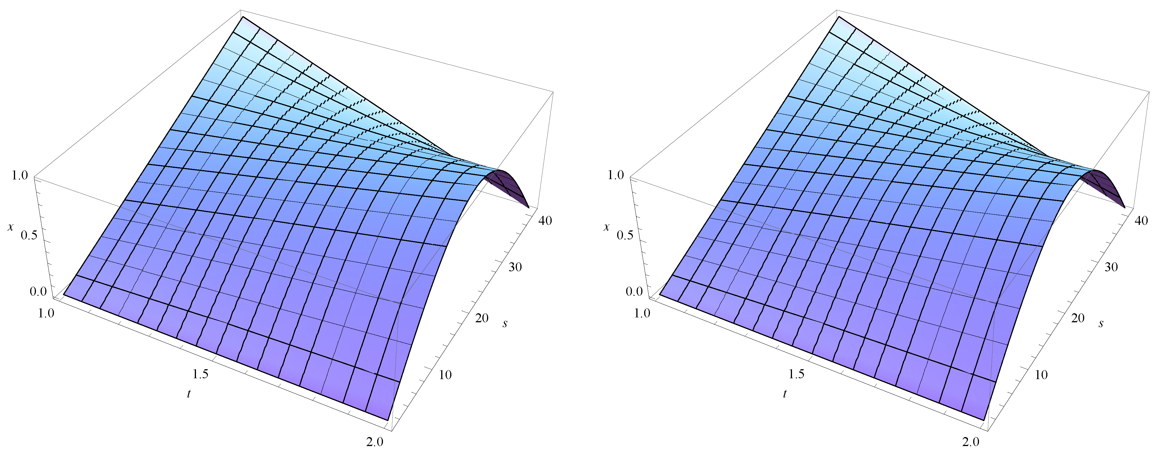
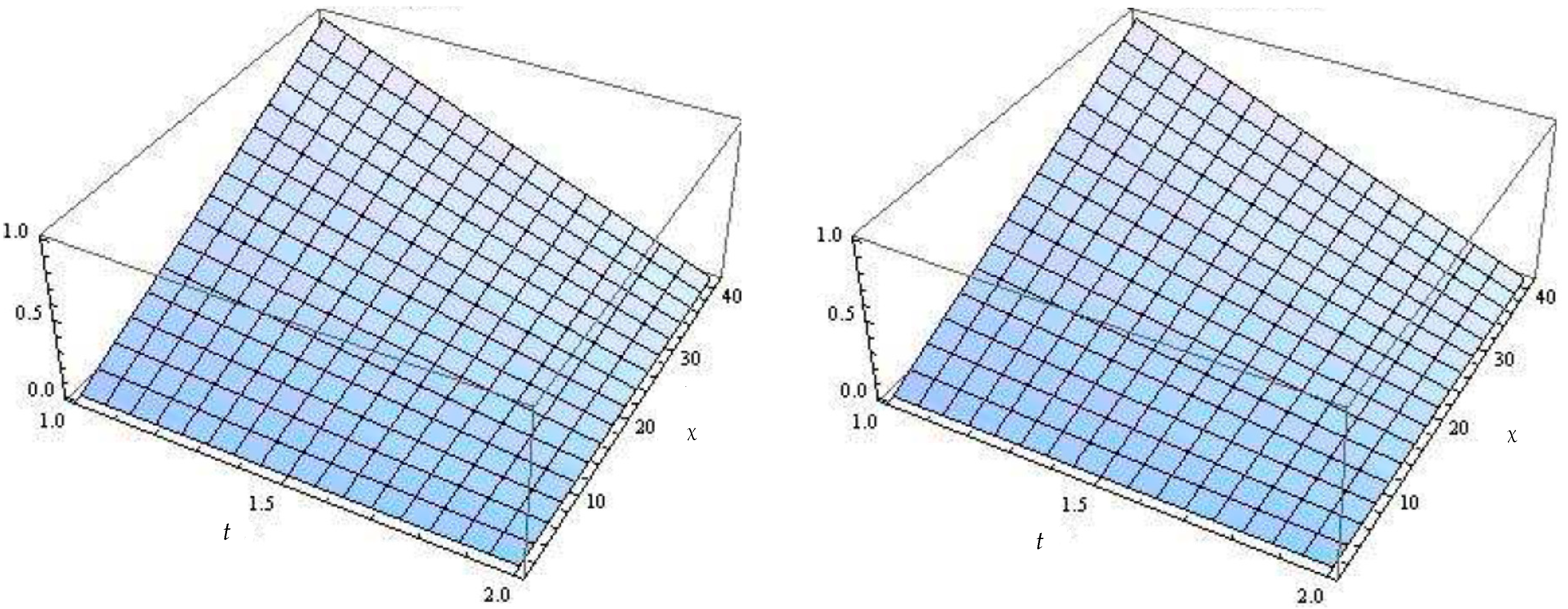
3. Results and Discussion

In this section, two numerical examples of proposed method are presented to check the accuracy, effectiveness, and correctness of the proposed approach by adding 3D graphs and some results in tabular form. 3D Graph technology is such a technique to be used for projecting multidimensional data/arrays into a visual form that is easier to understand, analyze and interpret, thus authors showed an accuracy of approximate solutions to the true solution by 3D plots. Mathematica and Matlab are used to do the computations using the steps given in Algorithm 1.

Algorithm 1:  Coding algorithm for the proposed scheme

Input b, N, k, K, and $\gamma$.  Step 1. Define each sextic spline segment $T_j\left(s\right)$.  Step 2. Construct consistency relation Equation (13) and two end Equations (14) and (15).  Step 3. Approximate Caputo FD at time $t=t_{n+1}$ as in Equation (17).  Step 4. Using the semi-discrete FD operator $V_t^{\gamma }$, the Equation (17) is converted to Equation (19).  Step 5. Using SPS for space discretization to convert Equations (19) to (43).  Step 6. Compute the elements of the vectors $\mathbf{v}$, $\mathbf{g}$, $\tilde{\mathbf{v}}$ and $\tilde{\mathbf{g}}$.  Step 7. Compute the elements of the matrices A, B and C.  Step 8. Compute the elements of the matrice ${\mathbf{P}}^{\mathbf{1}}=A^{-1}B(\mathbf{v}+\mathbf{g})+A^{-1}C(\tilde{\mathbf{v}}+\tilde{\mathbf{g}})$.   $\mathbf{Output}$ ${\chi }_n^K$

Example 1.

Consider a higher-order PDE

$$\begin{array}{ccc}\hfill \frac{{\partial }^{\gamma }\chi }{\partial t^{\gamma }}+\eta \frac{{\partial }^4\chi }{\partial s^4}& =& g(s,t),s\in [0,1],t\in (0,T],\hfill \end{array}$$

with the IC

$$\begin{array}{ccc}\hfill \chi (s,0)& =& sin\left(\pi s\right),s\in [0,1]\hfill \end{array}$$

and BCs

$$\begin{array}{ccc}\hfill {\chi (s,t)|}_{s=0}& =& {\chi (s,t)|}_{s=1}=0,\hfill \\ \hfill {\chi }_{ss}{(s,t)|}_{s=0}& =& {\chi }_{ss}{(s,t)|}_{s=1}=0,t\in [0,T],\hfill \end{array}$$

where $g(s,t)=sin\left(\pi s\right)t^{1-\gamma }{E}_{1,2-\gamma }\left(t\right)+\eta {\pi }^{4}exp\left(t\right)sin\left(\pi s\right)$ and $E_{\gamma ,\mu }\left(s\right)$ is the two parameter function of $Mittag$-Leffler type. The analytical solution of the proposed problem is

$$\begin{array}{ccc}\hfill \chi (s,t)& =& sin\pi sexp\left(t\right).\hfill \end{array}$$

The above equation yields the following equation when γ is one,

$$\begin{array}{ccc}\hfill \frac{\partial \chi }{\partial t}+\eta \frac{{\partial }^4\chi }{\partial s^4}& =& g(s,t),s\in [0,1],t\in [0,T].\hfill \end{array}$$

(54)

The $\gamma =0.75$ and $\eta =0.01$ are used to solve this problem. The greatest absolute $L_{\infty }$ and $L_2$ error norms for $k=40$ and $k=80$ with $\mathrm{\Delta }t=0.000001$ are reported in Table 1. To prevent contaminating spatial and temporal-discretization errors, $\mathrm{\Delta }t$ is set to a relatively modest value in this problem. The Kth time level is modified to assess the correctness of the presented approach, which demonstrates its efficiency. The suggested technique accurately approximates the analytical solution, as shown in Table 1. As illustrated in Figure 1, the numerical and precise solutions are displayed using $k=40$, $K=500$, and $\mathrm{\Delta }t$ = 0.000001.

Table 1. The error norms for various k when $\mathrm{\Delta }t$ = 0.000001.

$\gamma =0.75$	k	K	$\parallel e_K{\parallel }_{\infty }$	$\parallel e_K{\parallel }_2$
	40	100	$1.1389\times {10}^{-3}$	$1.2733\times {10}^{-4}$
		500	$4.0224\times {10}^{-3}$	$4.4972\times {10}^{-4}$
		1000	$6.9266\times {10}^{-3}$	$7.7442\times {10}^{-4}$
	80	100	$1.1389\times {10}^{-3}$	$9.0036\times {10}^{-5}$
		500	$4.0224\times {10}^{-3}$	$3.18\times {10}^{-4}$
		1000	$6.9266\times {10}^{-3}$	$5.476\times {10}^{-4}$
$\gamma =1$
	40	100	$1.9246\times {10}^{-4}$	$2.1518\times {10}^{-5}$
		500	$9.8211\times {10}^{-4}$	$1.098\times {10}^{-4}$
		1000	$1.9692\times {10}^{-3}$	$2.2016\times {10}^{-4}$
	80	100	$1.9246\times {10}^{-4}$	$1.5215\times {10}^{-5}$
		500	$9.8211\times {10}^{-4}$	$7.7642\times {10}^{-5}$
		1000	$1.9692\times {10}^{-3}$	$1.5568\times {10}^{-4}$

Figure 1. Numerical & analytical solutions when k = 40, K = 500 and $\gamma =0.75$ for Example 1.

Example 2.

Consider another higher-order PDE

$$\begin{array}{ccc}\hfill \frac{{\partial }^{\gamma }\chi }{\partial t^{\gamma }}+\eta \frac{{\partial }^4\chi }{\partial s^4}& =& g(s,t),s\in [0,1],0<t\le T,\hfill \end{array}$$

with the IC

$$\begin{array}{ccc}\hfill {\chi (s,t)|}_{t=0}& =& 0,s\in [0,1]\hfill \end{array}$$

and BCs

$$\begin{array}{ccc}\hfill {\chi (s,t)|}_{s=0}& =& {\chi (s,t)|}_{s=1}=0,\hfill \\ \hfill {\chi }_{ss}{(s,t)|}_{s=0}& =& {\chi }_{ss}{(s,t)|}_{s=1}=0,0\le t\le T,\hfill \end{array}$$

The true solution of the problem is

$$\begin{array}{ccc}\hfill \chi (s,t)& =& tsin\pi s.\hfill \end{array}$$

The above equation yields the following equation when γ is one,

$$\begin{array}{ccc}\hfill \frac{\partial \chi }{\partial t}+\eta \frac{{\partial }^4\chi }{\partial s^4}& =& g(s,t),s\in [0,1],t\in [0,T].\hfill \end{array}$$

(55)

Here $g(s,t)=sin\left(\pi s\right)\frac{1}{\mathrm{\Gamma }(2-\gamma )}{t}^{1-\gamma }+\eta {\pi }^{4}tsin\left(\pi s\right)$. The $\gamma =0.5$ and $\eta =0.05$ are used to solve this problem. The greatest absolute $L_{\infty }$ and $L_2$ error norms for $k=40$ and $k=80$ with $\mathrm{\Delta }t=0.000001$ are reported in Table 2. To prevent contaminating spatial and temporal-discretization errors, $\mathrm{\Delta }t$ is set to a relatively modest value in this problem. The Kth time level is modified to assess the correctness of the presented approach, which demonstrates its efficiency. The suggested technique accurately approximates the analytical solution, as shown in Table 2. As illustrated in Figure 2, the numerical and precise solutions are displayed using $k=40$, $K=500$, and $\mathrm{\Delta }t$ = 0.000001.

Table 2. The error norms for various k when $\mathrm{\Delta }t$ = 0.000001.

$\gamma =0.5$	k	K	$\parallel e_K{\parallel }_{\infty }$	$\parallel e_K{\parallel }_2$
	40	100	$9.9755\times {10}^{-5}$	$1.1153\times {10}^{-5}$
		500	$4.999\times {10}^{-4}$	$5.5891\times {10}^{-5}$
		1000	$9.9994\times {10}^{-4}$	$1.118\times {10}^{-4}$
	80	100	$9.9755\times {10}^{-5}$	$7.8863\times {10}^{-6}$
		500	$4.999\times {10}^{-4}$	$3.9521\times {10}^{-5}$
		1000	$9.9994\times {10}^{-4}$	$7.9052\times {10}^{-5}$
$\gamma =1$
	40	100	$9.7001\times {10}^{-5}$	$1.0845\times {10}^{-5}$
		500	$4.9701\times {10}^{-4}$	$5.5567\times {10}^{-5}$
		1000	$9.9701\times {10}^{-4}$	$1.1147\times {10}^{-4}$
	80	100	$9.7001\times {10}^{-5}$	$7.6686\times {10}^{-6}$
		500	$4.9701\times {10}^{-4}$	$3.9292\times {10}^{-5}$
		1000	$9.9701\times {10}^{-4}$	$7.8821\times {10}^{-5}$

Figure 2. Numerical and analytical solutions for Example 2 when k = 40, K = 500 and $\gamma =0.5$.

4. Conclusions

The fourth-order problems play a significant role in modern science and engineering and their solutions are need to be examined in order to understand the dynamical framework of plate-models of bridge slabs, floor systems, window glasses and airplane wings. The approximate solution of 4th-order EP with time-fractional CD has been accomplished using an SPST in this study. The time discretization has been done using the backward Euler formula. Sextic spline approach has been utilized for spatial derivative discretization. The approximate solution converges to the analytical solution with order $O({\rho }^4+\mathrm{\Delta }{t}^{2-\gamma })$. Numerical test applications have been presented to show the accuracy of the sextic spline technique. The presented scheme has been found to provide highly accurate results. The efficacy of the proposed techniques has been established by calculating the error norms for the obtained results.

References

- Podlubny, I. Fractional Differential Equations; Academic Press: New York, NY, USA, 1999. [Google Scholar]
- Oldham, K.B.; Spanier, J. The Fractional Calculus; Academic Press: New York, NY, USA, 1974. [Google Scholar]
- Berdyshev, A.S.; Eshmatov, B.E.; Kadirkulov, B.J. Boundary value problems for fourth-order mixed type equation with fractional derivative. Electron. J. Differ. Equ. 2016, 36, 1–11. [Google Scholar]
- He, J.H. A new fractal derivation. Therm. Sci. 2011, 15, 145–147. [Google Scholar] [CrossRef]
- Wang, K.L.; Wang, H. A novel variational approach for fractal Ginzburg-Landau equation. Fractals 2021, 29, 2150205-131. [Google Scholar] [CrossRef]
- Wang, K.L. Exact solitary wave solution for fractal shallow water wave model by He’s variational method. Mod. Phys. Lett. B 2021, 22, 2150602. [Google Scholar] [CrossRef]
- He, J.H.; Ji, F.Y. Two-scale mathematics and fractional calculus for thermodynamics. Therm. Sci. 2019, 23, 2131–2133. [Google Scholar] [CrossRef]
- Wang, K.L. A study of the fractal foam drainage model in a microgravity space. Math. Methods Appl. Sci. 2021, 44, 10530–10540. [Google Scholar] [CrossRef]
- Yang, X.H.; Xu, D.; Zhang, H.X. Crank-Nicolson/quasi-wavelets method for solving fourth order partial integro-differential equation with a weakly singular kernel. J. Comput. Phys. 2013, 234, 317–329. [Google Scholar] [CrossRef]
- Liu, Y.; Fang, Z.; Li, H.; He, S. A mixed finite element method for a time-fractional fourth-order partial differential equation. Appl. Math. Comput. 2014, 243, 703–717. [Google Scholar] [CrossRef]
- Khan, N.A.; Khan, N.U.; Ayaz, M.; Mahmood, A.; Fatima, N. Numerical study of timefractional fourth-order differential equations with variable coefficients. J. King Saud Univ. Sci. 2011, 23, 91–98. [Google Scholar] [CrossRef] [Green Version]
- Moghaddam, B.P.; Machado, J.A.T.; Behforooz, H. An integro quadratic spline approach for a class of variable-order fractional initial value problems. Chaos Solitons Fractals 2017, 102, 354–360. [Google Scholar] [CrossRef]
- Roul, P.; Goura, V.M.K.P.; Cavoretto, R. A numerical technique based on B-spline for a classof time-fractional diffusion equation. Numer. Methods Partial Differ. Equ. 2021, 1–20. [Google Scholar] [CrossRef]
- Abdeljawad, T.; Agarwal, R.P.; Karapinar, E.; Kumari, P.S. Solutions of the nonlinear integral equation and fractional differential equation using the technique of a fixed point with a numerical experiment in extended b-metric space. Symmetry 2019, 11, 686. [Google Scholar] [CrossRef] [Green Version]
- El-Sayed, A.A.; Baleanu, D.; Agarwal, P. A novel Jacobi operational matrix for numerical solution of multi-term variable-order fractional differential equations. J. Taibah Univ. Sci. 2020, 14, 963–974. [Google Scholar] [CrossRef]
- Hamasalh, F.K.; Muhammed, P.O. Computational non-polynomial spline function for solving fractional Bagely-Torvik equation. Math. Sci. Lett. 2017, 6, 83–87. [Google Scholar] [CrossRef]
- Pedas, A.; Vikerpuur, M. Spline Collocation for Multi-Term Fractional Integro-Differential Equations with Weakly Singular Kernels. Fractal Fract. 2021, 5, 90. [Google Scholar] [CrossRef]
- Youssri, Y.H. Orthonormal Ultraspherical Operational Matrix Algorithm for Fractal-Fractional Riccati Equation with Generalized Caputo Derivative. Fractal Fract. 2021, 5, 100. [Google Scholar] [CrossRef]
- Cardone, A.; Conte, D.; D’Ambrosio, R.; Paternoster, B. Multivalue Collocation Methods for Ordinary and Fractional Differential Equations. Mathematics 2022, 10, 185. [Google Scholar] [CrossRef]
- Lu, Z.; Zhu, Y. Numerical approach for solution to an uncertain fractional differential equation. Appl. Math. Comput. 2019, 343, 137–148. [Google Scholar] [CrossRef]
- Gao, W.; Veeresha, P.; Prakasha, D.G.; Baskonus, H.M.; Yel, G. A powerful approach for fractional Drinfeld-Sokolov-Wilson equation with Mittag-Leffler law. Alex. Eng. J. 2019, 58, 1301–1311. [Google Scholar] [CrossRef]
- Mirzaee, F.; Samadyar, N. Implicit meshless method to solve 2D fractionalstochastic Tricomi-type equation defined onirregular domain occurring in fractal transonic flow. Numer. Methods Partial Differ. Equ. 2021, 37, 1781–1799. [Google Scholar] [CrossRef]
- Shen, L.; Zhu, S.; Liu, B.; Zhang, Z.; Cui, Y. Numerical implementation of nonlinear system offractional Volterra integral-differential equations by Legendre wavelet method and error estimation. Numer. Methods Partial Differ. Equ. 2021, 37, 1344–1360. [Google Scholar] [CrossRef]
- Khan, W.A. Numerical simulation of Chun–Hui He’s iteration method with applications in engineering. Int. J. Numer. Methods Heat Fluid Flow 2022, 32, 944–955. [Google Scholar] [CrossRef]
- Bueno-Orovio, A.; Kay, D.; Burrage, K. Fourier spectral methods for fractional-in-space reaction-diffusion equations. BIT Numer. Math. 2014, 54, 937–954. [Google Scholar] [CrossRef]
- Arqub, O.A.; Shawagfeh, N. Application of reproducing kernel algorithm for solving Dirichlet time-fractional diffusion-Gordon types equations in porous media. J. Porous Media 2019, 22, 411–434. [Google Scholar] [CrossRef]
- Prakash, A.; Goyal, M.; Gupta, S. Fractional variational iteration method for solving time-fractional Newell-Whitehead-Segel equation. Nonlinear Eng. 2019, 8, 164–171. [Google Scholar] [CrossRef]
- Yaseen, M.; Abbas, M. An efficient computational technique based on cubic trigonometric B-splines for time fractional Burgers’ equation. Int. J. Comput. Math. 2020, 97, 725–738. [Google Scholar] [CrossRef] [Green Version]
- Mishra, H.K.; Nagar, A.K. He-Laplace method for linear and nonlinear partial differential equations. J. Appl. Math. 2012, 2012, 180315. [Google Scholar]
- Sene, N. Fractional diffusion equation described by the Atangana-Baleanu fractional derivative and its approximate solution. J. Fract. Calc. Nonlinear Syst. 2021, 2, 60–75. [Google Scholar] [CrossRef]
- Wahash, H.A.; Panchal, S.K. Positive solutions for generalized Caputo fractional differential equations using lower and upper solutions method. J. Fract. Calc. Nonlinear Syst. 2020, 1, 1–12. [Google Scholar] [CrossRef]
- Ji, P.Q.; Wang, J.; Lu, L.X.; Ge, C.F. Li-He’s modified homotopy perturbation method coupled with the energy method for the dropping shock response of a tangent nonlinear packaging system, Journal of Low Frequency Noise. Vib. Act. Control 2021, 40, 675–682. [Google Scholar]
Publisher’s Note: MDPI stays neutral with regard to jurisdictional claims in published maps and institutional affiliations. |
© 2022 by the authors. Licensee MDPI, Basel, Switzerland. This article is an open access article distributed under the terms and conditions of the Creative Commons Attribution (CC BY) license (https://creativecommons.org/licenses/by/4.0/).