Article

Novel Analytical Technique to Find Closed Form Solutions of Time Fractional Partial Differential Equations

1
Department of Mathematics, University of Wah, Wah Cantt 47040, Pakistan
2
Department of Mechanical Engineering, Sejong University, Seoul 05006, Korea
*
Author to whom correspondence should be addressed.
Fractal Fract. 2022, 6(1), 24; https://doi.org/10.3390/fractalfract6010024
Submission received: 24 November 2021 / Revised: 28 December 2021 / Accepted: 31 December 2021 / Published: 1 January 2022

Abstract

:
In this article, a new method for obtaining closed-form solutions of the simplified modified Camassa-Holm (MCH) equation, a nonlinear fractional partial differential equation, is suggested. The modified Riemann-Liouville fractional derivative and the wave transformation are used to convert the fractional order partial differential equation into an integer order ordinary differential equation. Using the novel (G′/G2)-expansion method, several exact solutions with extra free parameters are found in the form of hyperbolic, trigonometric, and rational function solutions. When parameters are given appropriate values along with distinct values of fractional order α travelling wave solutions such as singular periodic waves, singular kink wave soliton solutions are formed which are forms of soliton solutions. Also, the solutions obtained by the proposed method depend on the value of the arbitrary parameters H. Previous results are re-derived when parameters are given special values. Furthermore, for numerical presentations in the form of 3D and 2D graphics, the commercial software Mathematica 10 is incorporated. The method is accurately depicted, and it provides extra general exact solutions.

1. Introduction

Fractional calculus is a sort of fractional differential equation that resembles a large sweeping differential equation [1]. In the sense that many theoretical and practical characteristics of differential equations can be easily extended to fractional differential equations while maintaining the same character and spirit. In a letter to Leibniz in 1695, L’Hopital demanded a precise description of the derivative of order n = 0.5, sowing the seeds of fractional calculus almost 300 years ago. As a result, fractional integrals and derivatives differ from regular integrals and derivatives in a variety of ways, allowing them to be applied to a broader range of problems that integer-order calculus cannot adequately capture. In many branches of science and engineering, fractional calculus has been carefully developed to be a very authoritative approach to assist scientists in uncovering the hidden properties of the dynamics of multidimensional systems. Fractional calculus has played a crucial role in recent years as a proficient, efficient, and elementary theoretical basis for more accurate modelling of diverse dynamic processes. As a result, fractional calculus is being utilized more frequently in modelling, signal processing, physics, electromagnetics, biological systems, mechanics, medicine, biology, chemistry, bioengineering, and other domains [2,3]. Differential equations with non-integer derivatives [4] have been discovered lately. For example, fractional derivatives can be utilized to anticipate seismic nonlinear oscillations [5]. Nonlinear equations with multi-order fractional derivatives have recently been added to the list of applications. The complex transformation of fractional order is used to turn a fractional order nonlinear partial differential equation (FNPDE) into a nonlinear ordinary differential equation (NODE) [6,7]. Fractional order differential equations are well represented by a variety of significant phenomena in material science, electrochemistry, electromagnetics, and viscoelasticity [8,9]. Researchers [10,11] give a physical understanding of fractional calculus.
A soliton is a self-reinforcing wave packet that maintains its shape while propagating at a constant rate. Solitons, in other words, are unaffected by collisions with other solitons in terms of shape and speed, and are studied in nuclear physics, quantum mechanics, and waves along a weakly anharmonic mass-spring chain. Periodic travelling waves, among other things, play a role in self-oscillatory systems, reaction–diffusion–advection systems, and excitable chemical reactions. The motion of a particle in a potential field in the presence of dissipation is referred to as self-oscillatory dynamics. The described method of self-oscillation excitation is caused by features of a potential whose shape is dependent on the system state, rather than by characteristics of a dissipation function. Furthermore, properties of a potential function allow for self-oscillation excitation in the scenario where the dissipation function is positive at each phase space point. Reaction-diffusion-advection equations are partial differential equations that describe the evolution of a substance (e.g., a drug) in a medium described by spatial coordinates, involving sheltered transport (or advection) according to a physical or chemical force represented by a velocity vector, diffusion, or irregular motion of the material molecules in the medium, and reaction (e.g., chemical) with other constituents present in the medium represented by a reaction vector. They demonstrate physical properties such as the singular periodic wave solution, singular single-soliton solution, and singularly double periodic wave solution. The solutions’ features make them ideal for analyzing nonlinear processes in applied math, physics, and engineering.
The dynamics of waves in the fractional Schrödinger equation with harmonic potential were studied by Zhang et al. [12]. To explore such dynamics, they used an analytical technique with fractional Laplacian derivative and compared it to numerical simulation. They discovered that the beams follow zigzag and funnel-like patterns in one and two dimensions, which become irregular after a substantial period of propagation. In a fractional Schrödinger equation with a 𝒫𝒯-symmetric potential, Zhang et al. [13] explored the conical diffraction of a light beam. Their research not only shows how to acquire beam localization in a 𝒫𝒯-symmetric potential without using nonlinearities, but it also relates fractional Laplacian and symmetry, implying that their research has benefits on both sides. As a result, it could have a lot of potential for manufacturing on-chip optical devices. Through the longitudinal modulation of the transverse Gaussian and periodic potentials, Zhang et al. [14] also studied resonant mode conversions and Rabi oscillations in the fractional Schrödinger equation. They discovered that the Lévy index can efficiently alter the oscillation period and conversion efficiency.
As a result of the introduction of symbolic computation tools like Maple and Mathematica, various numerical and analytical approaches for searching accurate solutions of nonlinear evolution equations (NLEEs) have garnered further attention. Many approaches for obtaining exact solutions have been devised and established as a result, including the Cole-Hopf transformation [15], Tanh-function [16], Inverse scattering transform [17], Exp-function [18,19,20,21,22,23], differential transform [24], and Laplace perturbation [25], F-expansion [26] methods.
Wang et al. [27] recently proposed an expansion method called the (G′/G) -expansion, which they demonstrated to be a powerful method for finding analytic solutions to NLEEs. It is a trustworthy method for obtaining a wide range of solitary wave solutions, such as hyperbolic, trigonometric, and rational functions.
The (G′/G)-expansion approach recently become popular [28,29] has caught the interest of a large number of scientists. The method was used to create closed form solutions to a number of NPDEs. The travelling waves solutions of biological population model of fractional order, the Burgers equation with time-fractional order, and the space-time fractional Whitham–Broer–Kaup model were investigated by Arshed and Sadia [30] by using the (G′/G2)-expansion methodology in 2018. In 2020, the (G′/G2)-expansion method was used to build numerous novel accurate travelling wave solutions for the Boiti–Leon–Pempinelli system in two dimensions [31]. The unidirectional Dullin–Gottwald–Holm (DGH) system describing wave prorogation in shallow water, which include singular periodic wave solutions, shock-singular, shock, and singular solutions investigated in 2021 by Bilal et al. [32] to find novel exact solutions via the (G′/G2)- expansion approach.
A novel (G′/G2)-expansion method is introduced in this article, to solve the MCH equation of fractional order in the sense of Jumarie [33], and we discover a large number of new families of precise solutions. The proposed technique has never been reported in the literature previously which make it novel.
The Jumarie fractional order derivative of order α is demarcated by the expression:
D t α v ( t ) = { 1 Γ ( 1 α ) d d t 0 t ( t ς ) α ( v ( ς ) v ( 0 ) )   d ς ,       0 < α 1   , (   v ( n )   ( t )   ) ( α n )   ,                                                         n α < n + 1   ,       n 1
Properties of Jumarie’s fractional derivative are:
D t α f ( t ) = Γ     ( 1 + ω ) Γ     ( 1 + ω α )   t ω α ,
D t α   ( f ( t ) g ( t ) ) = g ( t ) D t α   f ( t ) + f ( t )   D t α g ( t )   ,
D t α h   [ g   ( t )   ] = h g [ g ( t ) ]   D t α   g ( t )   = D g α h [ g ( t ) ] ( g ( t ) ) α .

2. The Methodology

Assume that a fractional PDE has the form:
P   ( u ,   u x ,   u t , D t α u , ) = 0 ,             0 < α 1 ,
In which the unknown function is denoted by   u ( x , t ) .
The method’s main steps are as follows:
Step 1: The complex fractional transformation [7]
u   ( x , t )     = u ( η )   ,   η = L x + V t α Γ ( 1 + α ) ,    
In which L and V are arbitrary constants transforms Equation (5) into an ODE
M     ( u , u , u , u , ) = 0 ,
where ordinary derivatives with regard to η are denoted by superscripts.
Step 2: If possible, integrate Equation (7) one or more times to obtain integration constants that can be determined later.
Step 3: Assume the solution to Equation (7) can be categorized as follows:
u ( η ) = i = p p a i ( H + ( G / G 2 ) )   i ,
where a i and H are constants, found later, and G is the solution of following differential equation:
( G / G 2 ) = A + B ( G / G 2 ) 2
with A 1 and B 0 being integers.
Step 4: According to the balancing principle between the highest order derivative and the nonlinear term in Equation (7), the value of a positive integer p can be determined.
Step 5: We get polynomials in ( H + ( G / G 2 ) ) i , ( i = 0 ,   ± 1 ,   ± 2 ,   , ± p ) by substituting Equation (8) with Equation (9) into Equation (7). The system of algebraic equations is obtained by putting to zero each coefficient of the resultant polynomials. By solving system of equations with Maple, the values of the constants a i ( i = 0 ,   ± 1 ,   ± 2 ,   , ± p ) , H ,   L ,   C     and     V can be retrieved.
Step 6: On the base of the general solutions of Equation (9), the ratio G G 2 can be split into three categories:
G G 2 = A B ( E cos ( A B η ) + F sin ( A B η ) F cos ( A B η ) E sin ( A B η ) )   ,       A B > 0 ,
G G 2 = | A B | B ( E sinh ( 2 | A B | η ) + E cosh ( 2 | A B | η ) + F E sinh ( 2 | A B | η ) + E cosh ( 2 | A B | η ) F )   ,       A B < 0 ,
G G 2 = E B ( E η + F ) ,     A = 0 ,       B 0 ,
where E and F are constants that are not zero.

3. Application

Consider the following time fractional MCH equation:
D t α u + 2 δ   u x u x   x   t + ψ   u 2 u x = 0 ,       where     δ ,   ψ >   0 ,   0 < α 1 ,
where D t α is the Jumarie fractional derivative of order α ,   δ is a non-zero real constant, and ψ is a positive constant.
Many researchers have examined the simplified MCH equation and attempted to obtain exact answers in a number of approaches. For example, Liu et al. [34] are interested in solving the simplified MCH equation using the ( G / G ) -expansion method, with an auxiliary equation as linear ordinary differential equation (LODE) of second order. The sine-cosine approach was used on MCH equation by Wazwaz [35] to investigate the exact solutions. The ( G / G ) -expansion strategy was used to MCH problem in conjunction with the generalized Riccati equation by Zaman and Sultana [36] to obtain the closed form solutions.
Using Equation (4), we convert Equation (12) into an ODE, and integrating once, we get:
( V + 2 δ L )   u V L 2 u + + ψ L u 3 3 + C 1 = 0 ,
where C 1 is an integration constant that will be calculated later.
In Equation (14), we obtain p = 1 by applying the homogeneous balancing principle among the uppermost order derivative and the uppermost order nonlinear term. As a result, trial solution (8) is:
u ( η ) = a 1   ( H + ( G / G 2 ) ) 1 + a 0 + a 1     ( H + ( G / G 2 ) ) .
In equating the coefficients of all ( H + ( G / G 2 ) )   i , ( i = 0 ,   ± 1 ,   ± 2 ,   ± 3 ) , a system of equations for the unknowns a 0 ,   a 1 , a 1 , H , C 1 , V and L are given as by putting the left hand side of Equation (15) into Equation (14).
1 3 ψ L a 1 3 2 V L 2 a 1   B H 2 = 0 , 6 V L 2 a 1 B 2 H + ψ L a 0   a 1 2 = 0 , 2 δ L a 1 +   ψ L a 1 a 1 2 + V a 1 6 V L 2 a 1 B 2 H 2 2 V L 2 a 1 A B + + ψ L a 0 2 a 1   = 0 , 2 V L 2 a 1 A B H + 2 V L 2 a 1 B 2 H + 2   ψ L a 0 a 1 a 1 + V a 0 + 2 δ L a 0 + 1 3 ψ L a 0 3 + 2 V L 2 a 1 B 2 H 3 + C 1 = 0 , 2 δ L a 1 6 V L 2 a 1 B 2 H 2 + V a 1 + ψ L a 1 a 1 2 + ψ L a 1 + a 0 2 2 V L 2 a 1 A B = 0 , 6 V L 2 a 1 B 2 H 3 + ψ L a 0 a 1 2 + 6 V L 2 a 1 A B H = 0 , 1 3 ψ L a 1 3 2 V L 2 a 1 A 2 4 V L 2 a 1 A B H 2 2 V L 2 a 1 B 2 H 4 = 0 .
Using symbolic computation software to solve the given system of equations, we get the following results:
Set 1.
  a 0 = ± 6 δ B L H 3 ψ ( 4 L 2 A B + 6 L 2 B 2 H 2 + 1 ) ,   a 1 = ± 2 L 3 δ ( A + B H 2 ) ψ ( 4 L 2 A B + 6 L 2 B 2 H 2 + 1 ) δ ,   a 1 = 6   δ B L 3 ψ ( 4 L 2 A B + 6 L 2 B 2 H 2 + 1 ) ,     C 1 = ± 48 L 4 δ 2 B 2 H ( A + B H 2 ) 3 ψ δ ( 4 L 2 A B + 6 L 2 B 2 H 2 + 1 ) ( 4 L 2 A B + 6 L 2 B 2 H 2 + 1 ) ,     V = 2 δ L 4 L 2 A B + 6 L 2 B 2 H 2 + 1 ,   H = H .
Set 2.
  a 0 = 2 3 δ B L H ψ ( 2 L 2 A B 1 ) ,       a 1 = ± 2 3 ψ δ ( 2 L 2 A B 1 ) ( A + B H 2 ) L ψ ( 2 L 2 A B 1 ) ,   a 1 = 0 ,     C 1 = 0 ,     V = 2 δ L 2 L 2 A B 1 ,   H = H .
Set 3.
  a 0 = a 0 ,       a 1 = 0 ,   a 1 = ± 2   3 ψ δ ( 2 L 2 A B 1 ) B L ψ ( 2 L 2 A B 1 ) ,     C 1 = 0 ,     V = 2 δ L 2 L 2 A B 1 ,   H = a 0 3 ψ ( 2 L 2 A B 1 ) 6 ψ δ ( 2 L 2 A B 1 ) B L .
When the three cases with Equation (16) and the interleaving ratios Equations (10)–(12) are combined, there are three clusters of solutions for Equation (13):
Family 1. When A B > 0 , the trigonometric function solution of the Equation (13) is
u 11 ( η ) = ± 2 L 3 δ ( A + B H 2 ) ψ ( 4 L 2 A B + 6 L 2 B 2 H 2 + 1 ) δ   ( H + A B ( E cos ( A B η ) + F sin ( A B η ) F cos ( A B η ) E sin ( A B η ) ) ) 1                                 6   δ B L 3 ψ ( 4 L 2 A B + 6 L 2 B 2 H 2 + 1 )     ( H + A B ( E cos ( A B η ) + F sin ( A B η ) F cos ( A B η ) E sin ( A B η ) ) )                                   ± 6 δ B L H 3 ψ ( 4 L 2 A B + 6 L 2 B 2 H 2 + 1 ) ,
where η = L x 2 δ L t α ( 4 L 2 A B + 6 L 2 B 2 H 2 + 1 )   ( Γ ( 1 + α ) ) .
When A B < 0 , the solution of Equation (13) is:
u 12 ( η ) = ± 2 L 3 δ ( A + B H 2 ) ψ ( 4 L 2 A B + 6 L 2 B 2 H 2 + 1 ) δ   ( H | A B | B ( E sinh ( 2 | A B | η ) + E cosh ( 2 | A B | η ) + F E sinh ( 2 | A B | η ) + E cosh ( 2 | A B | η ) F ) ) 1                                 6   δ B L 3 ψ ( 4 L 2 A B + 6 L 2 B 2 H 2 + 1 )     ( H | A B | B ( E sinh ( 2 | A B | η ) + E cosh ( 2 | A B | η ) + F E sinh ( 2 | A B | η ) + E cosh ( 2 | A B | η ) F ) )                                 ± 6 δ B L H 3 ψ ( 4 L 2 A B + 6 L 2 B 2 H 2 + 1 ) ,
where η = L x 2 δ L t α ( 4 L 2 A B + 6 L 2 B 2 H 2 + 1 )   ( Γ ( 1 + α ) ) .  
When A = 0 ,     B 0 , the solution of the Equation (13) is:
u 13 ( η ) = ± 2 L 3 δ ( A + B H 2 ) ψ ( 4 L 2 A B + 6 L 2 B 2 H 2 + 1 ) δ   ( H E B ( E η + F ) ) 1 ± 6 δ B L H 3 ψ ( 4 L 2 A B + 6 L 2 B 2 H 2 + 1 )                                 6   δ B L 3 ψ ( 4 L 2 A B + 6 L 2 B 2 H 2 + 1 )     ( H E B ( E η + F ) )   ,
where η = L x 2 δ L t α ( 4 L 2 A B + 6 L 2 B 2 H 2 + 1 )   ( Γ ( 1 + α ) ) .  
Family 2. When A B > 0 , the solution of the Equation (13) is:
u 21 ( η ) = 2 3 δ B L H ψ ( 2 L 2 A B 1 ) ± 2 3 ψ δ ( 2 L 2 A B 1 ) ( A + B H 2 ) L ψ ( 2 L 2 A B 1 )   ( H + A B ( E cos ( A B η ) + F sin ( A B η ) F cos ( A B η ) E sin ( A B η ) ) ) 1 ,
where η = L x + 2 δ L t α ( 2 L 2 A B 1 )   Γ ( 1 + α ) .  
When A B < 0 , the solution of the Equation (13) is:
u 22 ( η ) = ± 2 3 ψ δ ( 2 L 2 A B 1 ) ( A + B H 2 ) L ψ ( 2 L 2 A B 1 )   ( H | A B | B ( E sinh ( 2 | A B | η ) + E cosh ( 2 | A B | η ) + F E sinh ( 2 | A B | η ) + E cosh ( 2 | A B | η ) F ) ) 1                                   2 3 δ B L H ψ ( 2 L 2 A B 1 )   ,
where η = L x + 2 δ L t α ( 2 L 2 A B 1 )   Γ ( 1 + α ) .   .
When A = 0 ,     B 0 , the solution of the Equation (13) is:
u 23 ( η ) = 2 3 δ B L H ψ ( 2 L 2 A B 1 ) ± 2 3 ψ δ ( 2 L 2 A B 1 ) ( A + B H 2 ) L ψ ( 2 L 2 A B 1 )   ( H E B ( E η + F ) ) 1 ,
where η = L x + 2 δ L t α ( 2 L 2 A B 1 )   Γ ( 1 + α ) .  
Family 3. When A B > 0 , the solution of the Equation (13) is:
u 31 ( η ) =   a 0 ± 2   3 ψ δ ( 2 L 2 A B 1 ) B L ψ ( 2 L 2 A B 1 )     ( a 0 3 ψ ( 2 L 2 A B 1 ) 6 ψ δ ( 2 L 2 A B 1 ) B L + A B ( E cos ( A B η ) + F sin ( A B η ) F cos ( A B η ) E sin ( A B η ) ) )   ,
where η = L x + 2 δ L t α ( 2 L 2 A B 1 )   Γ ( 1 + α ) .  
When A B < 0 , the solution of the Equation (13) is:
u 32 ( η ) = a 0 ± 2   3 ψ δ ( 2 L 2 A B 1 ) B L ψ ( 2 L 2 A B 1 )     ( a 0 3 ψ ( 2 L 2 A B 1 ) 6 ψ δ ( 2 L 2 A B 1 ) B L | A B | B ( E sinh ( 2 | A B | η ) + E cosh ( 2 | A B | η ) + F E sinh ( 2 | A B | η ) + E cosh ( 2 | A B | η ) F ) ) .
where η = L x + 2 δ L t α ( 2 L 2 A B 1 )   Γ ( 1 + α ) .  
When A = 0 ,     B 0 , the solution of the Equation (13) is:
u 33 ( η ) = a 0 ± 2   3 ψ δ ( 2 L 2 A B 1 ) B L ψ ( 2 L 2 A B 1 )   ( a 0 3 ψ ( 2 L 2 A B 1 ) 6 ψ δ ( 2 L 2 A B 1 ) B L E B ( E η + F ) )   ,
where η = L x + 2 δ L t α ( 2 L 2 A B 1 )   Γ ( 1 + α ) .  
The main advantage of the presented method is that it offers more general and enormous amount of new exact traveling wave solutions when we take different values to p with some free parameters. The exact solutions have its extensive importance to interpret the inner structures of the natural phenomena. The explicit solutions represented various types of solitary wave solutions according to the variation of the physical parameters.

4. Results and Discussion

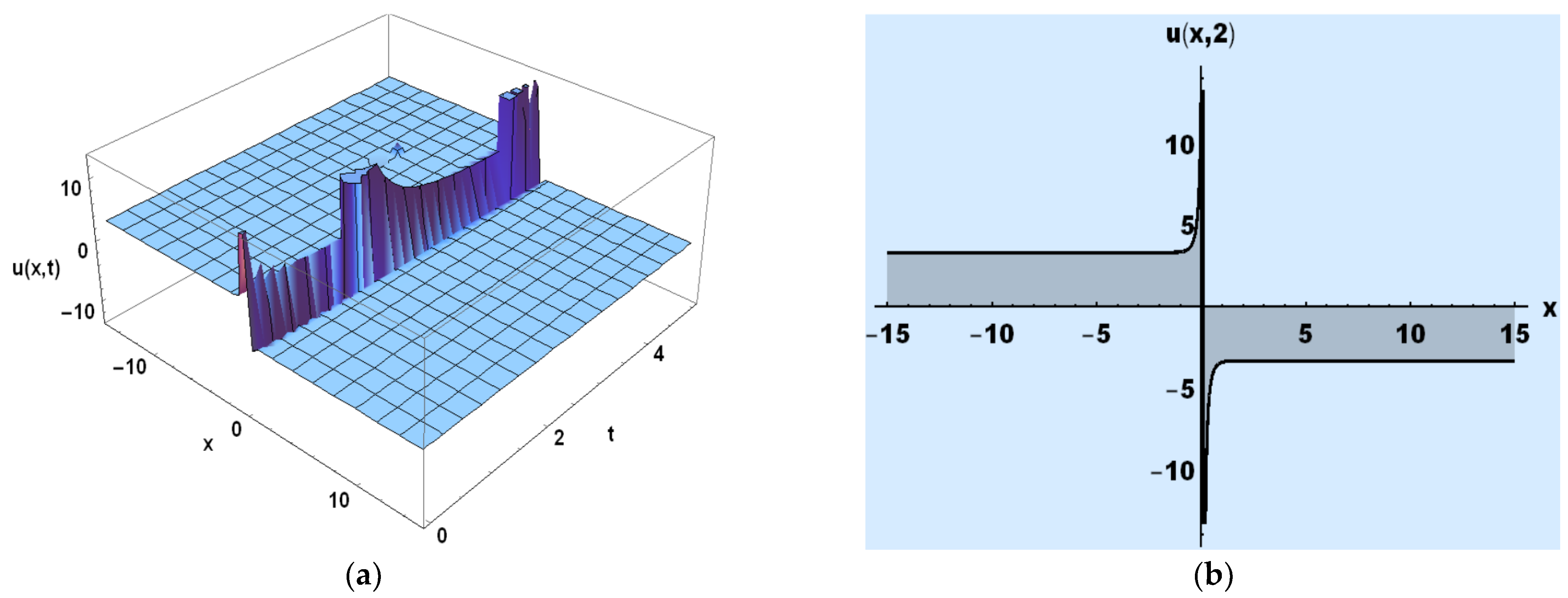
The found solution of the time fractional simplified MCH equation was described in this section. We get the travelling wave solutions assembled from Equations (19)–(27) to the time fractional simplified MCH equation using the novel (G′/G2)-expansion approach. The time-fractional order α for the equations is changed in order to study graphical behaviors of the exact solutions chosen from the preceding section. Mainly, the value of the time-fractional order used for the following simulations is α =   0.75 . Solutions u 11 ( η ) ,   u 12 ( η ) ,   u 21 ( η ) ,   u 22 ( η ) ,   u 31 ( η )   and u 32 ( η ) of Equation (13) are selected to present in terms of 3D, and 2D plots according to the values of α . The 3D solution graphs of u 11 ( η )   , and u 31 ( η )   are portrayed on the domain { ( x , t )   :     5 x 5 ,     0 t 1 }   , of   u 12 ( η ) on the domain { ( x , t )   :     5 x 5 ,     0 t 2 }   , of   u 21 ( η ) on the domain { ( x , t )   :     5 x 5 ,     0 t 5 }   , of   u 22 ( η ) on the domain { ( x , t )   :     15 x 15 ,     0 t 5 }   , and of   u 32 ( η ) on the domain { ( x , t )   :     20 x 20 ,     0 t 1 }   , respectively.
The 2D solution graphs, representing a relation among u(x) and x, of u 11 ( η )   is represented on { ( x , t )   :     5 x 5 ,     t = 0.2 }   , of   u 12 ( η )   , and   u 21 ( η ) on { ( x , t )   :     5 x 5 ,     t = 1 }   , of   u 22 ( η ) on { ( x , t )   :     15 x 15 ,     t = 2 }   , of   u 31 ( η ) on { ( x , t )   :     5 x 5 ,     t = 0.1 }   , and of   u 32 ( η ) on { ( x , t )   :     20 x 20 ,     t = 0.2 }   , 
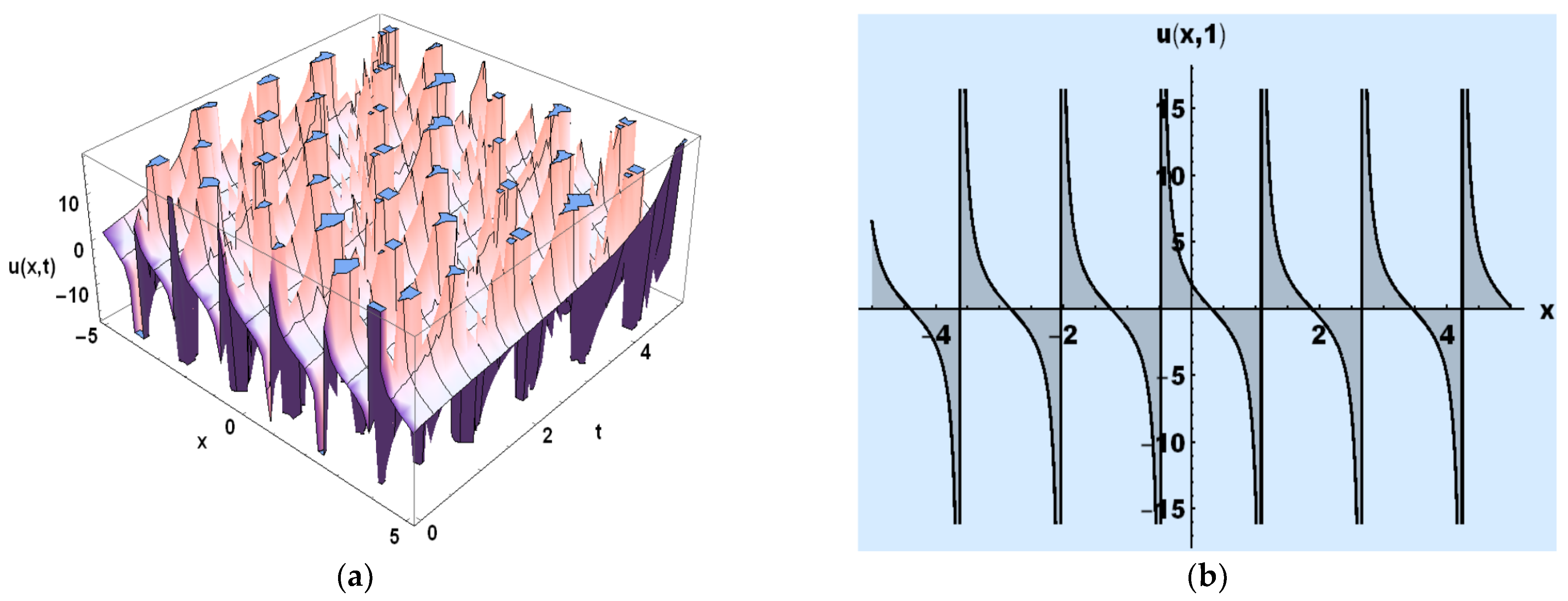
respectively. The solutions are singular periodic wave solution, and singular kink shape soliton, which are all generic solitary wave solutions. The solutions (19), (22) and (25) provide singular periodic wave solutions while, the solutions (20), (23), and (26) provide singular kink shape wave solutions, and the solutions (21), (24), and (27) provide rational solutions, according to the aforementioned solutions. 
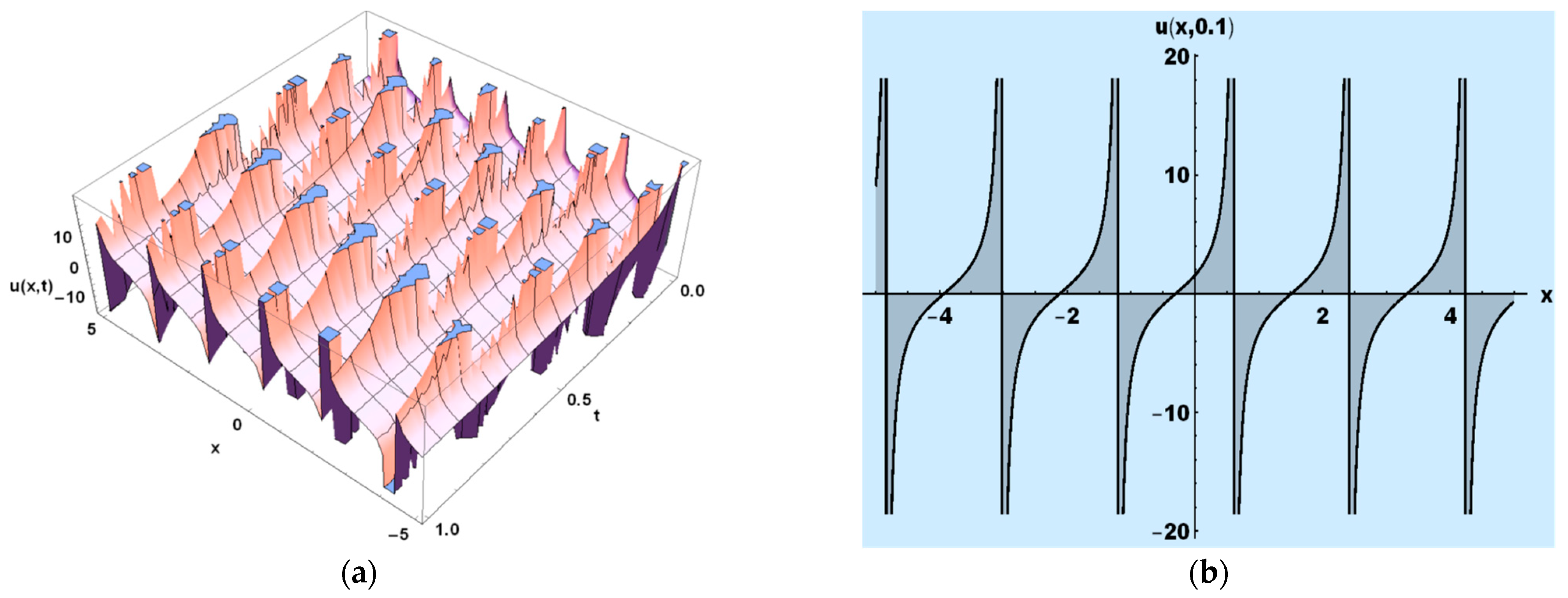
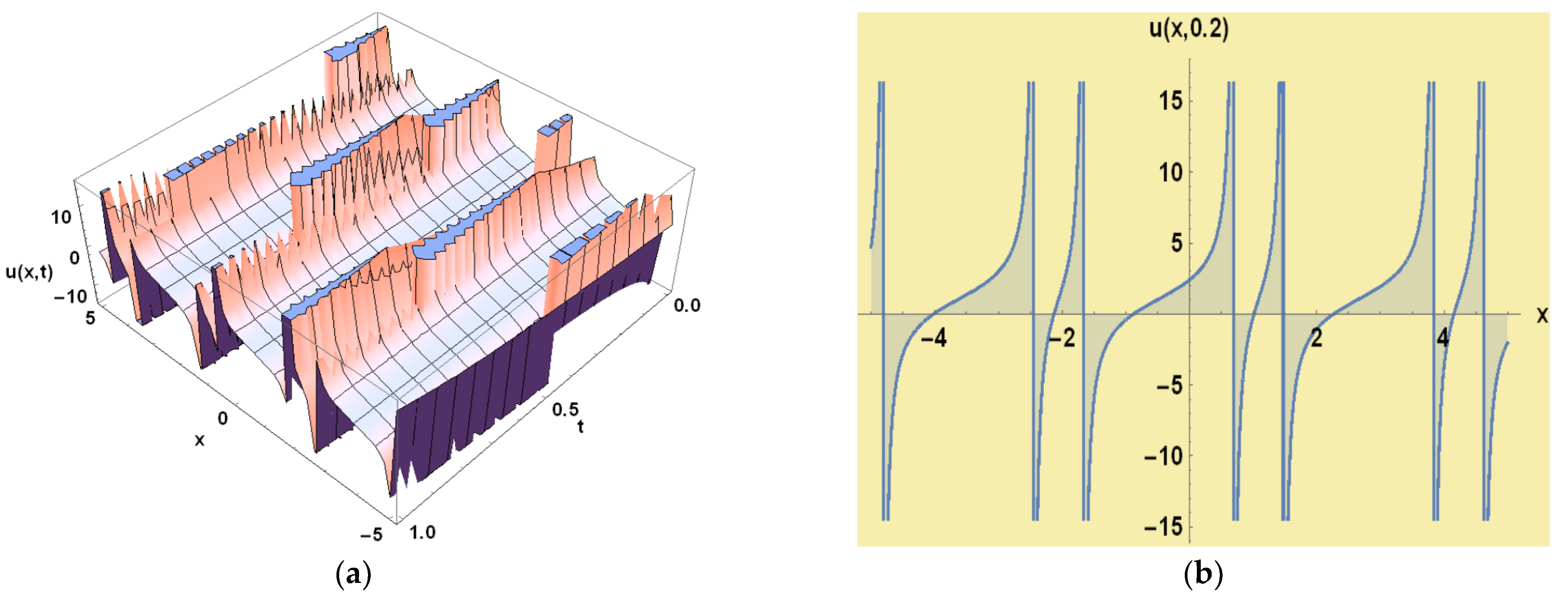
Figure 1a,b represents the singular periodic wave solution, which is spatiotemporal oscillations with discontinuous derivatives of u 11 ( η ) in Equation (19) for the parameters values A = 2 ,   B = 1 ,   E = 1 ,   F = 1 ,   H = 1 ,   ψ = 1 ,   δ = 1 , L = 1 in 3D and 2D. The Figure 2a,b and Figure 3a,b are similar to Figure 1a,b for different values of the parameters. 
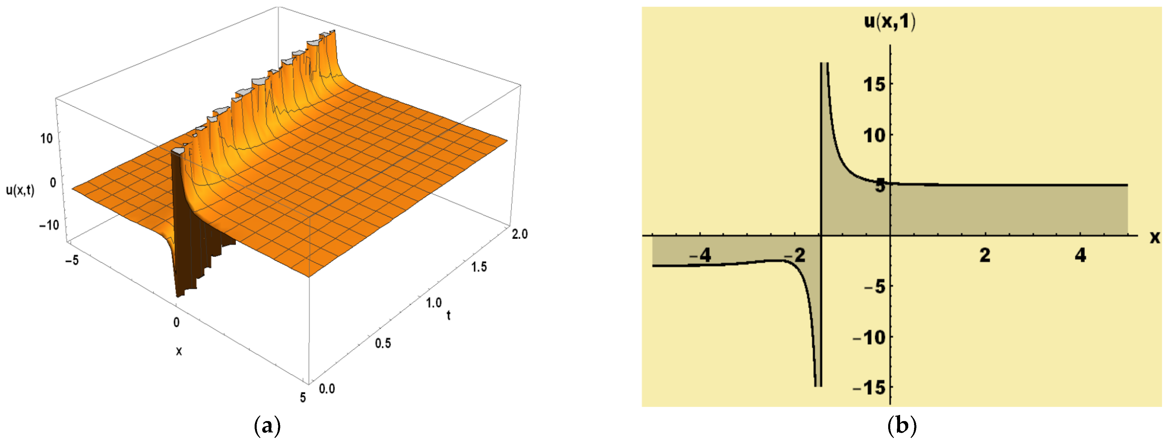
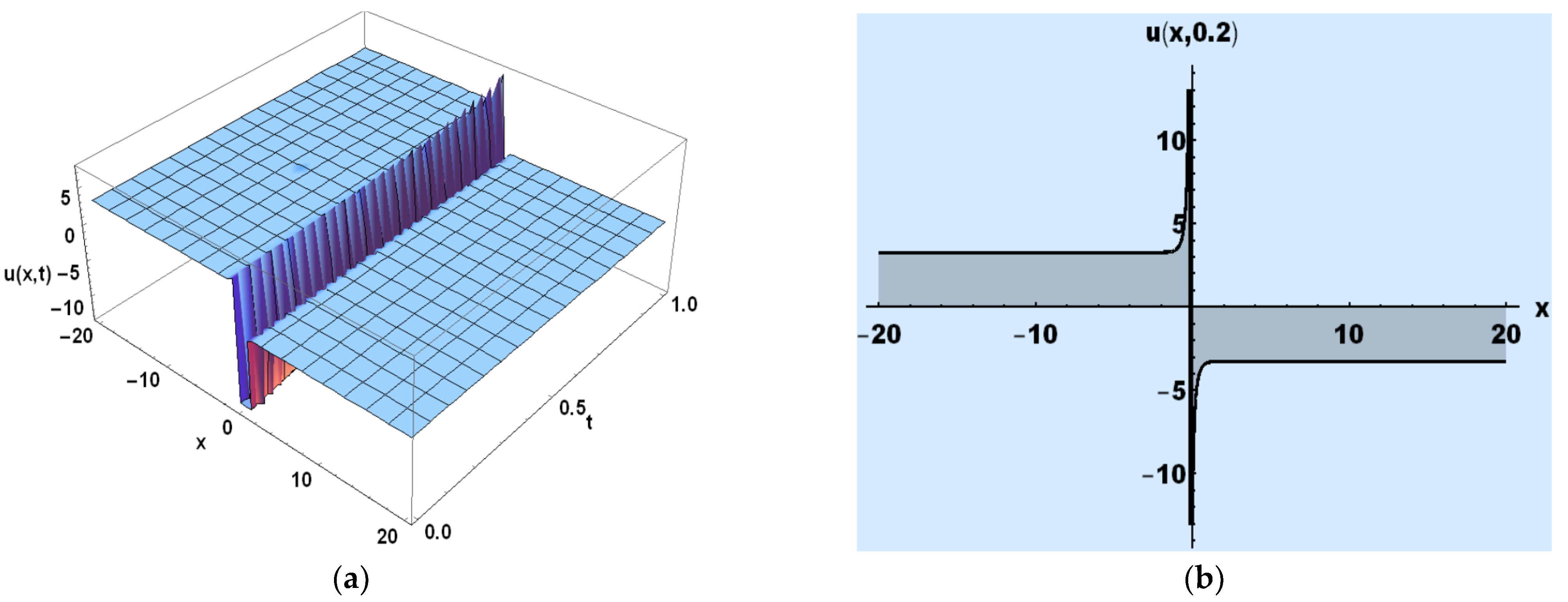
Figure 4a,b represents the 3-dimensional and 2-dimensional singular kink wave solution u 12 ( η ) in Equation (20) for the parameters values A = 2 ,   B = 3 ,   E = 1 , F = 1 ,   H = 2 ,     ψ = 2 ,   δ = 4.5 , L = 1 . Figure 5a,b and Figure 6a,b are similar to Figure 4a,b for different values of the parameters.
Comparison between our obtained solutions and the Liu et al. solutions [34].
Our Obtained SolutionsLiu et al. Solutions [34]
If   L = 1 ,   α = 1 ,   δ = 1 ,   A = 2 ,   B = 0.5 ,   E = 0 ,   ψ = 1 ,  
a 0 = 0 , and   u 31 ( ξ ) = u 3 , 4 ( x , t ) then our solution   u 31 ( ξ ) becomes:   u 3 , 4 ( x , t ) = ± 2 3 tan ( x + 2 t ) .
If we put C 1 = 1 ,   C 2 = 0 ,   λ 2 4 μ = 4 ,   and   k = 1 ,  
a = 1   in u 3 , 4 ( x , t ) then   u 3 , 4 ( x , t ) = ± 2 3 tan ( x + 2 t ) .
If L = 1 ,   α = 1 ,   δ = 1 ,   A = 2 ,   B = 0.5 ,   E = 1 ,   ψ = 1 ,  
a 0 = 0 ,   F = 0 and   u 33 ( ξ ) = u 3 , 4 ( x , t ) then our solution   u 33 ( ξ ) becomes:   u 3 , 4 ( x , t ) = ± 2 3 1 x + 2 t .
If we put   C 1 = 1 ,   C 2 = 1 ,   λ = 2 , μ = 1 ,   and   k = 1 ,  
a = 1 in   u 5 ( ξ ) then   u 3 , 4 ( x , t ) = ± 2 3 1 x + 2 t .
If L = 1 2 ,   α = 1 ,   δ = 2 ,   A = 2 ,   B = 2 ,   E = 0 ,   ψ = 4 ,  
a 0 = 0 , and   u 31 ( ξ ) = u 3 , 4 ( x , t ) then our solution   u 31 ( ξ ) becomes:   u 3 , 4 ( x , t ) = ± 6 i tan 1 2 ( x 4 t ) .
If we put   C 1 = 1 ,   C 2 = 0 ,   λ = 0 , μ = 1 4 ,   and   k = 1 ,  
a = 1 in   u 3 ( ξ ) then   u 3 , 4 ( x , t ) = ± 6 i tan 1 2 ( x 4 t ) .
If   L = 1 ,   α = 1 ,   δ = 1 ,   A = 2 ,   B = 0.5 ,   F = 0 ,   ψ = 1 ,  
a 0 = 0 ,   E = 1 and   u 33 ( ξ ) = u 3 , 4 ( x , t ) then our solution   u 33 ( ξ ) becomes:   u 3 , 4 ( x , t ) = ± 2 3 i 1 x 2 t .
If we put   C 1 = 1 ,   C 2 = 1 ,   λ = 2 , μ = 1 ,   and   k = 1 ,  
a = 1 in   u 5 ( ξ ) then   u 3 , 4 ( x , t ) = ± 2 3 i 1 x 2 t .

5. Conclusions

The time fractional simplified MCH problem is solved using a novel (G′/G2)-expansion method. Following the elimination of the trivial and excluded solutions, Equation (13) provides three types of solutions: trigonometric, exponential, and rational function solutions. The Maple software package was used to replace all of the exact answers created in this work back into their respective equations, and their fulfilment validated the correctness of the solutions provided in the current paper. After illustrating the graphs of numerous solutions for the value of α =   0.75 they demonstrate physical properties such as the singular periodic wave solutions, and singular kink wave solutions. The solutions’ features make them ideal for analyzing nonlinear processes in applied math, physics, and engineering. A soliton, for example, is a self-reinforcing wave packet that maintains its shape while propagating at a constant rate. Solitons, in other words, are unaffected by collisions with other solitons in terms of shape and speed, and are studied in nuclear physics, quantum mechanics, and waves along a weakly anharmonic mass-spring chain. Singular periodic travelling waves, among other things, play a role in self-oscillatory systems, reaction–diffusion–advection systems, and excitable chemical reactions. To conclusion, the method produces some truly unusual forms of solutions, and its performance is clear, direct, dependable, and successful. The limitation of the proposed method is that, it depends on the value of arbitrary constant H which can be calculated when the transformed ODE contains the constant of integration. As a result, we conclude that the provided approach can be used to address a wide range of NPDEs emerging in solitons theory or other physics and engineering areas. Finally, future research could benefit from applying the novel(G′/G2)-expansion approach to the proposed challenges involving an extension to the NLEEs involving sequential fractional partial derivatives.

Author Contributions

Conceptualization, M.S. and N.A.S.; methodology, J.D.C.; software, and validation, M.S., N.A.S. and J.D.C.; formal analysis and investigation, M.S.; resources, N.A.S.; writing—original draft preparation, M.S.; writing—review and editing, N.A.S.; supervision, J.D.C.; funding acquisition, J.D.C. All authors have read and agreed to the published version of the manuscript.

Funding

This research was supported by Basic Science Research Program through the National Research Foundation of Korea (NRF) funded by the Ministry of Education (No. 2017R1D1A1B05030422).

Institutional Review Board Statement

Not applicable.

Informed Consent Statement

Not applicable.

Data Availability Statement

Data sharing is not applicable to this article as no data set were generated or analyzed during the current study.

Conflicts of Interest

The authors declare that there is no conflict of interest regarding the publication of this paper.

References

  1. Nikitin, G.; Barannyk, T.A. Solitary waves and other solutions for nonlinear heat equations. Cent. Eur. J. Math. 2005, 2, 840–858. [Google Scholar] [CrossRef]
  2. Baleanu, D.; Machado, J.A.T.; Chen, W. Fractional differentiation and its applications I. Comput. Math. Appl. 2013, 66, 575. [Google Scholar] [CrossRef]
  3. Baleanu, D.; Garra, R.; Petras, I. Fractional variational approach to the fractional Basset-type equation. Rep. Math. Phys. 2013, 72, 57–64. [Google Scholar] [CrossRef]
  4. Podlubný, I. Fractional Differential Equations; Academic Press: San Diego, CA, USA, 1999. [Google Scholar]
  5. He, J.H. Some applications of nonlinear fractional differential equations and their applications. Bull. Sci. Technol. Soc. 1999, 15, 86–90. [Google Scholar]
  6. Li, Z.B.; He, J.H. Application of the fractional complex transform to fractional differential equations. Nonlinear Sci. Lett. A 2011, 2, 121–126. [Google Scholar]
  7. Li, Z.B.; He, J.H. Fractional complex transform for fractional differential equations. Math. Comput. Appl. 2010, 15, 970–973. [Google Scholar] [CrossRef] [Green Version]
  8. Baleanu, D.; Diethelm, K.; Scalas, E.; Trujillo, J.J. Fractional Calculus Models and Numerical Methods; World Scientific Publishing Company: Singapore, 2012. [Google Scholar]
  9. Das, S.; Kumar, R.; Gupta, P.K.; Jafari, H. Approximate analytical solutions for fractional space-and time-partial differential equations using homotopy analysis method. Appl. Appl. Math. Int. J. 1641, 2010, 5–659. [Google Scholar]
  10. Das, S. A note on fractional diffusion equations. Chaos Solitons Fractals 2009, 42, 2074–2079. [Google Scholar] [CrossRef]
  11. Yang, X.J. Advanced Local Fractional Calculus and Its Applications; World Science: New York, NY, USA, 2012. [Google Scholar]
  12. Zhang, Y.; Liu, X.; Belić, M.R.; Zhong, W.; Zhang, Y.; Xao, M. Propagation dynamics of a light beam in a fractional Schrödinger equation. Phys. Rev. Lett. 2015, 115, 180403. [Google Scholar] [CrossRef]
  13. Zhang, Y.; Zhong, H.; Belic, M.R.; Zhu, Y.; Zhong, W.; Zhang, Y.; Christodoulides, D.N.; Xiao, M. PT—Symmetry in a fractional Schrödinger equation. Laser Photonics Rev. 2016, 10, 526–531. [Google Scholar] [CrossRef] [Green Version]
  14. Zhang, Y.; Wang, R.; Zhong, H.; Zhang, J.; Belic, M.R.; Zhang, Y. Resonant mode conversions and Rabi oscillations in a fractional Schrödinger equation. Opt. Express 2017, 25, 32401–32410. [Google Scholar] [CrossRef]
  15. Salas, H.; Gomez, C.A. Application of the Cole-Hopf transformation for finding exact solutions to several forms of the seventh-order KdV equation. Math. Probl. Eng. 2010, 2010, 194329. [Google Scholar] [CrossRef]
  16. Malfliet, W. The tanh method: A tool for solving certain classes of nonlinear evolution and wave equations. J. Comput. Appl. Math. 2004, 164, 529–541. [Google Scholar] [CrossRef] [Green Version]
  17. Ablowitz, M.J.; Clarkson, P.A. Solitons, Nonlinear Evolution Equations and Inverse Scattering Transform; Cambridge University Press: Cambridge, UK, 1991. [Google Scholar]
  18. He, J.H.; Wu, X.H. Exp-function method for nonlinear wave equations. Chaos Solitons Fractals 2006, 30, 700–708. [Google Scholar] [CrossRef]
  19. Shakeel, M.; Iqbal, M.A.; Din, Q.; Hassan, Q.M.; Ayub, K. New exact solutions for coupled nonlinear system of ion sound and Langmuir waves. Indian J. Phys. 2020, 94, 885–894. [Google Scholar] [CrossRef]
  20. Hassan, Q.M.U.; Ahmad, J.; Shakeel, M. A novel analytical technique to obtain kink solutions for higher order nonlinear fractional evolution equations. Abstr. Appl. Anal. 2014, 2014, 213482. [Google Scholar] [CrossRef]
  21. Shakeel, M.; Mohyud-Din, S.T.; Iqbal, M.A. Closed form solutions for coupled nonlinear Maccari system. Comput. Math. Appl. 2018, 76, 799–809. [Google Scholar] [CrossRef]
  22. Baskonus, H.M. Dark and trigonometric soliton solutions in asymmetrical Nizhnik-Novikov-Veselov equation with (2 + 1)-dimensional. Int. J. Optim. Control. Theor. Appl. 2021, 11, 92–99. [Google Scholar] [CrossRef]
  23. Duran, S.; Askin, M.; Sulaiman, T.A. New soliton properties to the ill-posed Boussinesq equation arising in nonlinear physical science. Int. J. Optim. Control Theor. Appl. 2017, 7, 240–247. [Google Scholar] [CrossRef]
  24. Sarp, Ü.; Evirgen, F.; Ikikardes, S. Applications of differential transformation method to solve systems of ordinary and partial differential equations. J. Balıkesir Univ. Inst. Sci. Technol. 2018, 20, 135–156. [Google Scholar]
  25. Yavuz1, M.; Ozdemir, N.; Baskonus, H.M. Solutions of partial differential equations using the fractional operator involving Mittag-Leffler kernel. Eur. Phys. J. Plus 2018, 133, 215. [Google Scholar] [CrossRef]
  26. Wang, M.; Li, X. Applications of F-expansion to periodic wave solutions for a new Hamiltonian amplitude equation. Chaos Solitons Fractals 2005, 24, 1257–1268. [Google Scholar] [CrossRef]
  27. Wang, M.; Li, X.; Zhang, J. The (G′/G)-expansion method and travelling wave solutions of nonlinear evolution equations in mathematical physics. Phys. Lett. A 2008, 372, 417–423. [Google Scholar] [CrossRef]
  28. Hayward, R.; Biancalana, F. Constructing new nonlinear evolution equations with supersymmetry. J. Phys. A Math. Theor. 2018, 51, 275202. [Google Scholar] [CrossRef] [Green Version]
  29. Mohyud-Din, S.T.; Bibi, S. Exact solutions for nonlinear fractional differential equations using (G′/G2)-expansion method. Alex. Eng. J. 2018, 57, 1003–1008. [Google Scholar] [CrossRef]
  30. Arshed, S.; Sadia, M. (G′/G2)-expansion method: New traveling wave solutions for some nonlinear fractional partial differential equations. Opt. Quantum Electron. 2018, 50, 123. [Google Scholar] [CrossRef]
  31. Devi, P.; Singh, K. Exact traveling wave solutions of the (2 + 1)-dimensional Boiti-Leon-Pempinelli system using (G′/G2)-expansion method. AIP Conf. Proc. 2020, 2214, 020030. [Google Scholar]
  32. Bilal, M.; Seadawy, A.R.; Younis, M.; Rizvi, S.; Zahed, H. Dispersive of propagation wave solutions to unidirectional shallow water wave Dullin–Gottwald–Holm system and modulation instability analysis. Math. Methods Appl. Sci. 2021, 44, 4094–4104. [Google Scholar] [CrossRef]
  33. Jumarie, G. Modified Riemann-Liouville derivative and fractional Taylor series of non-differential functions further results. Comput. Math. Appl. 2006, 51, 1367–1376. [Google Scholar] [CrossRef] [Green Version]
  34. Liu, X.; Tian, L.; Wu, Y. Application of (G′/G)-expansion method to two nonlinear evolution equations. Appl. Math. Comput. 2010, 217, 1376–1384. [Google Scholar] [CrossRef]
  35. Wazwaz, M. New compact and noncompact solutions for variants of a modified Camassa-Holm equation. Appl. Math. Comput. 2005, 163, 1165–1179. [Google Scholar] [CrossRef]
  36. Zaman, M.M.; Sultana, S. Traveling wave solutions for the nonlinear evolution equation via the generalized Riccati equation and the (G′/G)-expansion method. World Appl. Sci. J. 2013, 22, 396–407. [Google Scholar]
Figure 1. (a,b): Graphical analysis of Equation (19) for the values of the parameters A = 2 ,   B = 1 ,   E = 1 ,   F = 1 ,     H = 1 ,   ψ = 1 ,   δ = 1 ,   L = 1 ,   α = 0.75 ,   5 x 5 ,   0 t 1 , for 3D and t = 0.2 for 2D plots.
Fractalfract 06 00024 g001
Figure 2. (a,b): Graphical analysis of Equation (23) for the values of the parameters A = 2, B = 3 ,   E = 1 ,   F = 1 ,     H = 1 ,   ψ = 1 ,   δ = 2 ,   L = 1 ,   α = 0.75 ,   15 x 15 ,   0 t 5 for 3D and t = 2 for 2D plots.
Fractalfract 06 00024 g002
Figure 3. (a,b): Graphical analysis of Equation (20) for the values of the parameters A = 2, B = 3 ,   E = 1 ,   F = 1 ,     H = 2 ,   ψ = 2 ,   δ = 4.5 ,   L = 1 ,   α = 0.75 ,   5 x 5 ,   0 t 2 , for 3D and t = 1 for 2D plots.
Fractalfract 06 00024 g003
Figure 4. (a,b): Graphical analysis of Equation (25) for the values of the parameters a 0 = 2 ,   ψ = 1 ,   δ = 2 ,   L = 1 ,   α = 0.75 ,   5 x 5 ,   0 t 1 for 3D and t = 0.1 for 2D plots.
Fractalfract 06 00024 g004
Figure 5. (a,b): Graphical analysis of Equation (22) for the values of the parameters A = 2 ,   B = 2 ,   E = 1 ,   F = 1 ,     H = 1 ,   ψ = 1 ,   δ = 1 ,   L = 1 ,   α = 0.75 ,   5 x 5 ,   0 t 5 for 3D and t = 1 for 2D plots.
Fractalfract 06 00024 g005
Figure 6. (a,b): Graphical analysis of Equation (26) for the values of the parameters A = 2, a 0 = 2 ,     ψ = 1 ,   δ = 2 ,   L = 1 ,   α = 0.75 ,   20 x 20 ,   0 t 1 for 3D and t = 0.2 for 2D plots.
Fractalfract 06 00024 g006
Publisher’s Note: MDPI stays neutral with regard to jurisdictional claims in published maps and institutional affiliations.

