Joint Optimization of Route and Speed for Methanol Dual-Fuel Powered Ships Based on Improved Genetic Algorithm

Abstract

Effective route and speed decision-making can significantly reduce vessel operating costs and emissions. However, existing optimization methods developed for conventional fuel-powered vessels are inadequate for application to methanol dual-fuel ships, which represent a new energy vessel type. To address this gap, this study investigates the operational characteristics of methanol dual-fuel liners and develops a mixed-integer nonlinear programming (MINLP) model aimed at minimizing operating costs. Furthermore, an improved genetic algorithm (GA) integrated with the Nonlinear Programming Branch-and-Bound (NLP-BB) method is proposed to solve the model. The case study results demonstrate that the proposed approach can reduce operating costs by more than 15% compared to conventional route and speed strategies while also effectively decreasing emissions of CO₂, NOx, SOx, PM, and CO. Additionally, comparative experiments reveal that the designed algorithm outperforms both the GA and the Linear Interactive and General Optimizer (LINGO) solver for identifying optimal route and speed solutions. This research provides critical insights into the operational dynamics of methanol dual-fuel vessels, demonstrating that traditional route and speed optimization strategies for conventional fuel vessels are not directly applicable. This study provides critical insights into the optimization of voyage decision-making for methanol dual-fuel vessels, demonstrating that traditional route and speed optimization strategies designed for conventional fuel vessels are not directly applicable. It further elucidates the impact of methanol fuel tank capacity on voyage planning, revealing that larger tank capacities offer greater operational flexibility and improved economic performance. These findings provide valuable guidance for shipping companies in strategically planning methanol dual-fuel operations, enhancing economic efficiency while reducing vessel emissions.

1. Introduction

To reduce ship emissions, the International Maritime Organization (IMO) has established several policies, such as Emission Control Area (ECA) regulation and the 2020 Sulfur Limit Order (SLO) [1,2,3]. Moreover, the European Union (EU) has decided to include shipping in the carbon trading system (CTS) [4,5]. The details of the three main emission reduction regulations are shown in

Table 1. Details of the three main emission reduction regulations.

Regulations	Requirements	Application Area
ECAs	Ships must use fuels with a sulfur content of no more than 0.1%	Baltic Sea, North Sea and English Channel, North American, US Caribbean coasts, China coasts, Specific ports of South Korea
SLO	Ships must use fuels with a sulfur content of no more than 0.5%	Outside the ECA applicable area
CTS	Ships need to pay tax on carbon dioxide above a certain threshold.	Europe

. In the above scenarios, traditional fuel ships must use Marine Gas Oil (MGO, sulfur content ≤ 0.10%) inside ECAs, and Low-Sulfur Fuel Oil (LSFO, sulfur content ≤ 0.50%) outside ECAs. And the ships also need to pay for carbon emissions; that is, their operating costs have increased significantly.

Currently, many shipping companies and researchers are focused on clean alternative energy, such as liquefied natural gas (LNG), liquefied biogas (LBG), methanol from natural gas, and renewable methanol [6,7,8]. Methanol demonstrates significant advantages in reducing emissions of SOx, NOx, and particulate matter (PM) while offering superior safety compared to other clean fuels such as ammonia and hydrogen [9,10]. Additionally, methanol remains in a liquid state at ambient temperature, providing unparalleled benefits in storage, transportation, and the development of bunkering infrastructure, unlike liquid hydrogen, liquefied natural gas, Liquefied Petroleum Gas, and liquid ammonia, which require cryogenic or extremely low temperatures to maintain their liquid form [11,12,13]. As a result, methanol has emerged as a prominent choice for marine fuel among shipping companies. According to a Clarksons Research report, in 2023, out of all the global new shipbuilding orders, 539 vessels were equipped with alternative fuels, accounting for 45% of the total tonnage ordered. Among these, 130 were methanol-powered vessels, representing approximately 13% of the total orders by tonnage, making methanol the second most popular alternative fuel after LNG-powered ships [14].

Existing research on methanol dual-fuel-powered ships predominantly focuses on engine design and emission calculations, with limited attention given to operational strategies such as route and speed optimization. Currently, there are relatively few ports globally equipped with methanol bunkering infrastructure [15]. Furthermore, the price disparity between methanol and conventional fuels necessitates tailored route and speed decision-making frameworks for methanol dual-fuel-powered vessels. In response to these challenges, this study aims to develop an integrated route and speed optimization methodology specifically designed for methanol dual-fuel-powered ships, with the objective of assisting shipping companies in reducing operational costs and emissions.

The remainder of this paper is organized as follows. In Section 2, the gaps in the existing literature are summarized. In Section 3, the problem description is presented. Section 4 and Section 5 present the construction of the mathematical model and the solution procedure, respectively. In Section 6, case studies are provided to verify the effectiveness of the proposed method. Finally, concluding remarks are given in Section 7.

2. Literature Review

Ronen [16] highlighted that a ship’s daily fuel consumption is proportional to the cube of its speed, implying that reducing speed can significantly decrease fuel usage. Building on this principle, numerous studies have focused on optimizing ship speed and routing to reduce costs and enhance environmental benefits. Zhang et al. [17] developed a multi-objective optimization model incorporating real-world wind and wave conditions, employing a multi-objective particle swarm algorithm to derive Pareto optimal solutions. By integrating an improved Technique for Order Preference by Similarity to an Ideal Solution (TOPSIS) algorithm, they identified optimal speeds, achieving a balance between environmental and economic benefits. Tzortzis and Sakalis [18] utilized a particle swarm algorithm to optimize ship speed, combining short-term weather forecasts to improve long-term prediction accuracy, and they demonstrated approximately 2% fuel savings in container ship routes. Similarly, Hua et al. [19] proposed a genetic algorithm-based optimization model that adjusts speed allocation to maximize economic benefits while meeting Carbon Intensity Indicator (CII) requirements. Luo et al. [20] introduced a method incorporating dynamic weather conditions, validating its effectiveness in dry bulk shipping with fuel savings of 5.35% and 7.34% compared to constant-speed and static models, respectively. Marashian et al. [21] optimized sailing speed using dynamic programming, achieving up to 3% fuel savings. Huotari et al. [22] combined dynamic programming with convex optimization, further reducing fuel consumption by 1.1–3.5%. Zinci and Bura [23], based on real data from general cargo ships, found that slow steaming, despite increasing voyage duration and operational costs, significantly reduced fuel consumption and emissions, with optimized total voyage costs decreasing by 23.3%, showcasing dual economic and environmental benefits. Taskar et al. [24] evaluated fuel-saving potential under varying speeds, demonstrating that speed optimization algorithms could achieve up to 6% fuel savings across different seasons and weather conditions, with more pronounced effects at lower speeds. Luo et al. [25] proposed a weather forecast-based speed optimization framework, further validating the significant potential of integrating weather forecasts to reduce fuel consumption and greenhouse gas emissions. Li et al. [26] constructed a fuel consumption prediction model, applied Fisher’s optimal segmentation method to divide shipping routes, and used iterative optimization to determine speeds, achieving fuel savings of 2.4–5.4%.

Some researchers have focused on optimizing routes to enhance the safety and economic efficiency of ship navigation [27,28,29,30]. Others have concentrated on developing methods for the simultaneous optimization of routes and speeds. Ma et al. [31] proposed a novel hierarchical mapping strategy in 2023, utilizing a bi-level mapping intelligent optimization algorithm to synchronize ship route and speed optimization. This strategy adapts to different carbon tax models and weather conditions, demonstrating significant cost-efficiency advantages in both conventional and complex marine environments. Wei et al. [32] established a joint optimization model for routes and speeds in 2022, incorporating marine environmental and time window constraints to minimize fuel consumption. Their study showed that precise adjustments to optimal routes and speeds could achieve fuel savings ranging from 0.21% to 5.04%. Cheng [33] developed a pickup and delivery optimization model for tramp ships, integrating routes, speeds, and cargo using Danzig–Wolfe decomposition and branch-and-price algorithms to minimize emissions and reduce costs. Lashgari et al. [34] proposed a scenario-based stochastic linear integer programming model in 2021, optimizing routes, speeds, and refueling strategies to reduce fuel costs, lower emissions, and adapt to fuel price uncertainties.

Ma et al. [35] introduced a speed and route optimization model incorporating Emission Control Area (ECA) regulations. Although this approach may increase total voyage distance, it effectively reduces sailing distance within ECAs, pollution emissions, and overall operational costs. Subsequent studies [36,37] in 2021 combined ECA regulations with weather conditions, employing the Non-dominated Sorting Genetic Algorithm II (NSGA-II) and TOPSIS technique to derive Pareto optimal solutions, further reducing voyage costs and time. In the same year, Ma et al. [38] proposed a nonlinear mixed-integer programming model to simultaneously optimize ship speed, routes, and refueling strategies to comply with the ECA low-sulfur fuel requirements. Zhen et al. [39] developed a bi-objective mixed-integer programming model in 2020 to optimize liner routes and speeds, minimizing fuel costs and emissions both inside and outside ECAs and providing decision-makers with Pareto optimal solutions. Numerous studies have also employed methods such as XGBoost to address similar engineering challenges [40,41,42,43].

Few studies have optimized operational strategies for LNG dual-fuel ships, which are similar to methanol dual-fuel ships. Tan et al. [44] studied the refueling problem in LNG dual-fuel container liner shipping operations. Considering the limited LNG bunkering infrastructure, they developed a flexible bunkering model for LNG dual-fuel ships to minimize operational costs. This model allows ships to deviate from their scheduled routes to non-port of calls to bunker LNG and adjust their sailing speed to maintain their weekly frequency. He et al. [45] extended the above research by applying the same approach to study the refueling problem of LNG dual-fuel tramp ships under limited LNG bunkering infrastructure. Based on the characteristics of the problem, they developed a more efficient mathematical formulation to solve the proposed model. However, the above studies have yet to address the problem of jointly optimizing route and speed for a liner shipping vessel with a dual-fuel engine to reduce operational costs. Furthermore, existing research on LNG dual-fuel vessels has not considered the impact of LNG fuel tank capacity on sailing decisions. This study fills these gaps in the existing research.

Moreover, the existing literature primarily focuses on traditional fuel-powered vessels rather than methanol dual-fuel ships. Given the price disparity between methanol and conventional fuels, as well as the limited availability of methanol bunkering infrastructure at ports, the optimization of routes and speeds for methanol dual-fuel vessels involves distinct parameters, constraints, and objective models. Consequently, the methodologies proposed in the aforementioned studies are not directly applicable to methanol dual-fuel operations. This paper aims to develop a joint route and speed optimization method for methanol dual-fuel-powered ships with the goal of minimizing navigation costs. The two main contributions of the present research are as follows:

(1) An MINLP model was developed to minimize the total cost, with shipping routes and speeds as decision variables. The model incorporates constraints such as methanol bunkering port availability, price differentials between methanol and conventional fuel, and methanol fuel tank capacity.

(2) An improved GA integrated with the NLP-BB method is proposed to solve the MINLP model. The GA, with several strategies (crossover strategy with a correction method, mutation strategy based on 2-opt method, and elite strategy), is used to solve the ship route, that is, the port-of-call sequence, and then the NLP-BB method is used to solve for the ship speed. Comparative experiments reveal that the proposed algorithm outperforms both the GA and the LINGO solver.

3. Problem Description

Liner shipping routes represent one of the most prevalent modes of transportation within the maritime industry [46,47,48,49]. These routes are characterized by the deployment of designated vessels that adhere to fixed schedules and port rotations, operating at relatively stable freight rates to facilitate the conveyance of both passengers and cargo. For a specific liner route, the sequence of port calls and the sailing speed between ports are the two primary variables. In the case of methanol dual-fuel-powered ships, liner routes and speed profiles designed for conventional fuel-powered vessels may not be economically optimal. Taking a liner route with eight ports as an example, as illustrated in Figure 1a,b, the port-of-call sequence depicted in Figure 1a is optimal for traditional fuel-powered ships. However, if port 5 offers methanol at a more competitive price, the port-of-call sequence shown in Figure 1b may be more advantageous for methanol dual-fuel-powered ships. Moreover, the sailing speed between every two ports should also be adjusted.

By integrating critical factors such as methanol bunkering port availability and the price dynamics of methanol and LSFO, this study aims to develop an integrated route and speed optimization framework for methanol dual-fuel-powered vessels, with the objective of minimizing voyage costs.

4. Mathematical Model

4.1. Model Assumptions

For the purpose of facilitating the modeling process, the following assumptions are proposed:

(1) The vessel is capable of switching between methanol and LSFO as fuel sources; however, such transitions are exclusively permissible during port berthing periods. This constraint necessitates the consistent utilization of a single type of fuel throughout the voyage between two consecutive ports.

(2) The decisions regarding shipping routes and speeds are exclusively associated with the vessel’s navigation process. Consequently, this study confines its focus to the fuel consumption costs and emissions generated during the ship’s voyage [50].

(3) Vessels are able to replenish LSFO at any port of call, whereas the provisioning of methanol fueling services is contingent upon the availability of specialized infrastructure, thus limiting such operations to ports equipped with the requisite capabilities.

(4) The service time at a given port was assumed to be constant [50].

The above assumptions contribute to the development of a more accurate and efficient model. For instance, Assumption 2 specifies that this study focuses solely on fuel consumption during vessel navigation. While ship equipment also consumes fuel during berthing, such consumption does not influence route and speed optimization decisions. Therefore, excluding these factors simplifies the model without compromising the validity of the conclusions.

4.2. Model Variables and Parameters

Indices and sets:

i, j: Index of port.

R: Set of ports along the service route.

R^M: Ports providing methanol bunkering services.

k: The port that provides methanol bunkering services before i along a certain route.

Parameters:

W: Ship displacement, ton.

B: Admiralty constant.

ω: The power index of the relationship between fuel consumption and speed.

L_ij: Sailing distance between port i and port j, n miles.

P^M: The price of methanol bunkering for ships, USD.

P^L: The price of LSFO bunkering for ships, USD.

t_j: Service time at port j, hours.

$t_j^1$ Arrival time at port j, hours.

$T_j^{\mathit{max}}$: Upper time limit for a ship to arrive at port j, hours.

v_min: Lower limit of ship’s sailing speed, kn.

v_max: Upper limit of ship’s sailing speed, kn.

τ: Daily cost of the ship, USD/day.

η^L: Ship engine energy consumption rate of LSFO, g/kwh.

γ: Carbon tax rate (USD/ton).

ψ: Threshold of CO₂ emissions (ton).

LC^M: Lower calorific values of methanol, MJ/ton.

LC^L: Lower calorific values of LSFO, MJ/ton.

Q^M: Methanol tank capacity, ton.

Q^L: Fuel oil tank capacity, ton.

$E{F}_n^M$ Emission factor of type n pollutants when methanol is used as a fuel, ton/ton.

$E{F}_n^L$: Emission factor of type n pollutants when LSFO is used as a fuel, ton/ton.

Decision Variables:

x_ij: Binary variable: if the ship sails from port i to port j, it equals 1; otherwise, it equals 0.

v_ij: Ship sailing speed from port i to port j, kn.

z_ij: Binary variable: if the ship uses methanol as fuel when traveling from port i to port j, the variable equals 1; otherwise, it equals 0.

4.3. Ship Sailing Total Costs

4.3.1. Ship Fuel Consumption Cost

The fuel consumption cost of a ship is the product of fuel consumption and fuel price, where the relationship between fuel consumption and ship sailing speed follows a power function [51]:

$$p^L=0.7355{\displaystyle \frac{W^{2/3}{(v)}^{\omega }}{B}}$$

(1)

$$p^M={\displaystyle \frac{L{C}^L}{L{C}^M}}\cdot {\displaystyle \frac{0.7355W^{2/3}{\left(v\right)}^{\omega }}{B}}$$

(2)

The energy consumption of a ship during sailing can be considered the product of p and the duration of sailing, as expressed below:

$$q_{ij}^L={\displaystyle \frac{(1-z_{ij})L_{ij}}{v_{ij}}}\cdot {\eta }^L{p}^L{10}^{-6}$$

(3)

$$q_{ij}^M={\displaystyle \frac{z_{ij}{L}_{ij}}{v_{ij}}}\cdot {\eta }^M{p}^M{10}^{-6}$$

(4)

Therefore, the ship fuel consumption cost can be expressed as follows:

$$\begin{array}{c}Cos{t}_1={\displaystyle \sum _{i,j\in R}}(P^L\cdot q_{ij}^L+P^M\cdot q_{ij}^M)\\ ={\displaystyle {\displaystyle \sum }_{i,j\in R}}{\displaystyle \frac{0.7355L_{ij}{W}^{2/3}{(v_{ij})}^{\omega -1}{10}^{-6}}{B}}[(1-z_{ij})P^L{\eta }^L+{\displaystyle \frac{L{C}^L{P}^M{\eta }^M}{L{C}^M}}]\end{array}$$

(5)

4.3.2. Time Cost

In liner shipping operations, vessels incur costs such as depreciation, management fees, and crew wages during transportation services. These costs are linearly correlated with time, meaning the total time cost can be expressed as the product of the unit time cost and the voyage duration.

$$Cos{t}_2={\displaystyle \sum }_{i,j\in R}{\displaystyle \frac{\tau L_{ij}}{v_{ij}}}+\sum _{j\in R}\tau t_j$$

(6)

4.3.3. Carbon Emissions Cost

The CO₂ emissions of ships can be calculated as the product of the emission factor and fuel consumption, which can be expressed as follows:

$$\begin{array}{c}Emissio{n}_{C{O}_2}={\displaystyle \sum _{i,j\in R}}(E{F}^{L,C{O}_2}\cdot q_{ij}^L+E{F}^{M,C{O}_2}\cdot q_{ij}^M)\\ ={\displaystyle {\displaystyle \sum }_{i,j\in R}}{\displaystyle \frac{0.7355L_{ij}{W}^{2/3}{(v_{ij})}^{\omega -1}{10}^{-6}}{B}}[(1-z_{ij})E{F}^{L,C{O}_2}{\eta }^L+{\displaystyle \frac{L{C}^{L}E{F}^{M,C{O}_2}{\eta }^M}{L{C}^M}}]\end{array}$$

(7)

Moreover, as previously mentioned, the carbon trading policy serves as a primary mechanism for limiting ship carbon emissions, which involves two key parameters: the carbon emission threshold (ψ) and the carbon tax (γ). Thus, the carbon emissions cost can be expressed as follows:

$${Cost}_3=\mathsf{\gamma }({Emission}_{{CO}_2}-\psi )$$

(8)

4.3.4. Constraint Conditions of the Model

(1) Constraint on the port call sequence of liner ships

In liner shipping routes, each port can only be visited once by a specific vessel during a single voyage. Therefore, the following constraint must be satisfied for each port:

$$\sum _{j\in P}{x}_{ij}=1,\forall i\in R,i\ne j$$

(9)

$$\sum _{i\in P}{x}_{ij}=1,\forall j\in R,i\ne j$$

(10)

To prevent potential sub-tour phenomena, a sub-tour elimination constraint, commonly used in Traveling Salesman Problem (TSP) modeling, is introduced as follows:

$$\sum _{i,j\in P^{\prime }}{x}_{ij}\le |R^{\prime }|-1,\forall R^{\prime }\subseteq R,2\le |R^{\prime }|\le N$$

(11)

When the problem scale is large, particularly with a significant number of ports, enumerating all subsets can impose substantial computational burdens, making it challenging to solve using solvers like CPLEX. To address this, an auxiliary variable θ_i is introduced to represent the number of ports visited by the vessel, transforming Equation (11) into the following form:

$${\theta }_i\le {\theta }_j+M(1-x_{ij})-1,\forall i,j\in R,j\ne 1,i\ne j$$

(12)

In Equation (12), M represents a sufficiently large positive number. Here, the nearest upper bound of M is adopted, i.e., M = |P|, to enhance computational efficiency. Consequently, Equation (12) can be simplified as follows:

$${\theta }_i\le {\theta }_j+|R|(1-x_{ij})-1,\forall i,j\in R,j\ne 1,i\ne j$$

(13)

$${\theta }_1=0$$

(14)

$${\theta }_i\in [1,|R|-1],\forall i\in R$$

(15)

(2) Fuel consumption constraint

When vessels operate using LSFO, their consumption must not exceed the corresponding tank capacity [52]. Therefore, the fuel consumption constraint of LSFO can be summarized as follows:

$${\displaystyle \frac{(1-z_{ij})L_{ij}}{v_{ij}}}\cdot {\eta }^L{p}^L{10}^{-6}\le Q^L,\forall i,j\in R$$

(16)

It should be noted that only some ports are equipped with the infrastructure to provide methanol bunkering services for ships. Therefore, the fuel consumption constraint of methanol can be summarized as follows:

$${\sum }_{i=k}^{i=k+j-1}{\displaystyle \frac{z_{i,i+1}{L}_{i,i+1}}{v_{i,i+1}}}\cdot {\eta }^M{p}^M{10}^{-6}\le Q^M,\forall k\in R^M$$

(17)

4.3.5. Objective Model

Based on Equations (1)–(17), the mathematical model aimed at minimizing vessel voyage costs can be summarized as follows:

$$\begin{array}{c}minCost=Cos{t}_1+Cos{t}_2+Cos{t}_3\\ ={\displaystyle {\displaystyle \sum }_{i,j\in R}}{\displaystyle \frac{0.7355L_{ij}{W}^{2/3}{(v_{ij})}^{\omega -1}{10}^{-6}}{B}}[(1-z_{ij})(P^L+\gamma E{F}^{L,C{O}_2}){\eta }^L+{\displaystyle \frac{L{C}^L(P^M+\gamma E{F}^{M,C{O}_2}){\eta }^M}{L{C}^M}}]\\ +{\displaystyle {\displaystyle \sum }_{i,j\in R}}{\displaystyle \frac{\tau L_{ij}}{v_{ij}}}+{\displaystyle {\displaystyle \sum }_{j\in R}}\tau t_j-\gamma \phi \end{array}$$

(18)

subjected to the following constraints:

$$\sum _{j\in P}{x}_{ij}=1,\forall i\in R,i\ne j$$

(19)

$$\sum _{i\in P}{x}_{ij}=1,\forall j\in R,i\ne j$$

(20)

$${\theta }_i\le {\theta }_j+|R|(1-x_{ij})-1,\forall i,j\in R,j\ne 1,i\ne j$$

(21)

$${\theta }_1=0$$

(22)

$${\theta }_i\in [1,|R|-1],\forall i\in R$$

(23)

$${\displaystyle \frac{0.7355L_{ij}{\eta }^L{W}^{2/3}{10}^{-6}}{B}}(1-z_{ij}){(v_{ij})}^{\omega -1}\le Q^L,\forall i,j\in R$$

(24)

$${\sum }_{i=k}^{i=k+j-1}{\displaystyle \frac{0.7355z_{i,i+1}{L}_{i,i+1}{\eta }^{M}L{C}^L{W}^{2/3}{10}^{-6}}{L{C}^{M}B}}{(v_{i,i+1})}^{\omega -1}\le Q^M,\forall k\in R^M$$

(25)

$$t_1^1=0$$

(26)

$$t_j^1+t_j+{\displaystyle \frac{L_{ij}}{v_{ij}}}\le T_j^{max},\forall i,j\in R$$

(27)

$$v_{min}\le v_{ij}\le v_{max},\forall i,j\in R$$

(28)

$$x_{ij}\in \left\{\mathrm{0,1}\right\},\forall i,j\in R$$

(29)

$$z_{ij}\in \left\{\mathrm{0,1}\right\},\forall i,j\in R$$

(30)

Constraints (19)–(23) ensure that the port call sequence adheres to liner shipping rules; constraints (24) and (25) guarantee that fuel consumption does not exceed tank capacity; constraints (26) and (27) ensure that the vessel arrives at each port within the agreed time frame; and constraints (28)–(30) define the feasible ranges of the decision variables.

5. Solution Method

5.1. Model Analysis

In Equations (18)–(30), the model includes both binary variables (x_ij and z_ij) and continuous variables (v_ij), along with multiple nonlinear terms in the objective function and constraints. As a result, the overall model constitutes an MINLP problem. Currently, many studies address this by transforming the MINLP model into a Mixed-Integer Linear Programming (MILP) model, which is then solved using solvers such as CPLEX and LINGO [53,54,55]. However, determining the port-of-call sequence can be categorized as a TSP. It is well known that the TSP is NP-hard, meaning the computational time increases exponentially with the number of ports the vessel must visit.

Numerous studies have demonstrated that genetic algorithms are an effective approach for solving NP-hard problems. Therefore, this study employs a genetic algorithm to determine the port-of-call sequence (x_ij), while the sailing speed and fuel switching variables (v_ij and z_ij) are solved using LINGO.

5.2. Algorithm Overview

The GA is a metaheuristic optimization technique inspired by the principles of natural selection and evolution [56,57]. It operates by iteratively developing a population of candidate solutions through processes such as selection, crossover, and mutation [58]. However, directly applying the GA to solve the port arrival sequence, i.e., the TSP, is often inefficient. Therefore, we propose an improved version of the GA, with the enhancement strategies outlined as follows:

Improved Crossover Strategy: Conventional genetic algorithms often employ sequential crossover to generate new offspring. However, the resulting offspring may contain duplicate ports. As illustrated in Figure 2a, for parent 1 and parent 2, selecting crossover points a1 and a2 produces offspring 1 and offspring 2, which fail to visit all ports.

To address this issue, a correction method is proposed: the port sequence between a1 and a2 is deleted, and the remaining portion of parent 2 is inserted in reverse order into the corresponding segment of parent 1. The same operation is performed on parent 2, yielding the new individuals shown in Figure 2b. It is evident that the modified crossover strategy ensures all ports are visited effectively.

Improved mutation strategy: Similarly to the crossover operation, traditional mutation strategies can also result in offspring individuals that fail to visit all ports. Therefore, in this study, the 2-opt method is used to change the sequence of two adjacent ports, which can be seen in Figure 3.

Elite strategy: Genetic operations do not always produce superior offspring. To effectively preserve the best individuals in each generation, the individual with the lowest objective function value is directly retained in the next generation without undergoing crossover or mutation.

5.3. Model Reformulation

For a specific genetic algorithm individual, the liner route is determined; that is, the port-call-sequence variable (x_ij) is known. At this point, only the remaining two variables, v_ij and z_ij, need to be determined. To facilitate description, several new parameters are defined as follows:

$${\lambda }^L={\displaystyle \frac{0.7355W^{2/3}{\eta }^L{10}^{-6}}{B}}$$

(31)

$${\lambda }^M={\displaystyle \frac{0.7355W^{2/3}{\eta }^{M}L{C}^L{10}^{-6}}{L{C}^{M}B}}$$

(32)

$${\rho }^L=P^L+\gamma E{F}^{L,C{O}_2}$$

(33)

$${\rho }^L=P^L+\gamma E{F}^{L,C{O}_2}$$

(34)

$$\delta ={\sum }_{j\in R}\tau t_j-\lambda \phi$$

(35)

where λ^L and λ^M represent the coefficients in the power function relationship between the fuel consumption and speed of LSFO and methanol, respectively; λ^L and λ^M represent the unit usage costs of LSFO and methanol, respectively; and δ represents other fixed costs. Then, x_ij is determined, and the above parameters are constants.

Since z_ij is a binary variable, the relaxation operation is as follows:

$${(z_{ij})}^2-z_{ij}=0,\forall i,j\in R$$

(36)

$$z_{ij}\ge 0,\forall i,j\in R$$

(37)

Therefore, the objective model can be rewritten as follows:

$$\begin{array}{c}minCost=Cos{t}_1+Cos{t}_2+Cos{t}_3\\ =\sum _{i,j\in R}{L}_{ij}{(v_{ij})}^{\omega -1}[{\lambda }^L{\rho }^L(1-z_{ij})+{\lambda }^M{\rho }^M{z}_{ij}]+{\displaystyle \sum }_{i,j\in R}{\displaystyle \frac{\tau L_{ij}}{v_{ij}}}+\delta \end{array}$$

(38)

subject to the following constraints:

$${\lambda }^L{L}_{ij}(1-z_{ij}){(v_{ij})}^{\omega -1}\le Q^L,\forall i,j\in R$$

(39)

$$\sum _{i=k}^{i=k+j-1}{\lambda }^M{z}_{i,i+1}{L}_{i,i+1}{(v_{i,i+1})}^{\omega -1}\le Q^M,\forall k\in R^M$$

(40)

$$t_1^1=0$$

(41)

$$t_j^1+t_j+{\displaystyle \frac{L_{ij}}{v_{ij}}}\le T_j^{max},\forall i,j\in R$$

(42)

$$v_{min}\le v_{ij}\le v_{max},\forall i,j\in R$$

(43)

$${(z_{ij})}^2-z_{ij}=0,\forall i,j\in R$$

(44)

$$z_{ij}\ge 0,\forall i,j\in R$$

(45)

To further analyze the properties of the transformed objective function, we introduce the following theorem:

Theorem 1.

The objective function cost is a convex function of v_ij and z_ij.

Proof of Theorem 1.

First, the first-order derivatives of cost with respect to v_ij and z_ij are calculated.

$${\displaystyle \frac{\partial Cost}{\partial v_{ij}}}=\sum _{i,j\in R}(\omega -1)L_{ij}{(v_{ij})}^{\omega -2}[{\lambda }^L{\rho }^L(1-z_{ij})+{\lambda }^M{\rho }^M{z}_{ij}]-\sum _{i,j\in R}\tau L_{ij}{(v_{ij})}^{-2}$$

(46)

$${\displaystyle \frac{\partial Cost}{\partial z_{ij}}}=\sum _{i,j\in R}{L}_{ij}{(v_{ij})}^{\omega -1}({\lambda }^M{\rho }^M-{\lambda }^L{\rho }^L)$$

(47)

The second-order derivatives of cost with respect to v_ij and z_ij are then calculated as follows:

$${\displaystyle \frac{{\partial }^{2}Cost}{\partial {(v_{ij})}^2}}={\sum }_{i,j\in R}(\omega -1)(\omega -2)L_{ij}{(v_{ij})}^{\omega -3}[{\lambda }^L{\rho }^L(1-z_{ij})+{\lambda }^M{\rho }^M{z}_{ij}]+{\sum }_{i,j\in R}\tau L_{ij}{(v_{ij})}^{-3}$$

(48)

$${\displaystyle \frac{{\partial }^{2}Cost}{\partial {(z_{ij})}^2}}=0$$

(49)

$${\displaystyle \frac{{\partial }^{2}Cost}{\partial (v_{ij})\partial (z_{ij})}}={\displaystyle \frac{{\partial }^{2}Cost}{\partial (z_{ij})\partial (v_{ij})}}={\sum }_{i,j\in R}(\omega -1)L_{ij}{(v_{ij})}^{\omega -2}({\lambda }^M{\rho }^M-{\lambda }^L{\rho }^L)-{\sum }_{i,j\in R}\tau L_{ij}{(v_{ij})}^{-2}$$

(50)

The Hessian matrix of the objective function is as follows:

$${\mathsf{\Delta }}^{2}Cost=|\begin{array}{cc}{\displaystyle \frac{{\partial }^{2}Cost}{\partial {(v_{ij})}^2}}& {\displaystyle \frac{{\partial }^{2}Cost}{\partial (v_{ij})\partial (z_{ij})}}\\ {\displaystyle \frac{{\partial }^{2}Cost}{\partial {(z_{ij})}^2}}& {\displaystyle \frac{{\partial }^{2}Cost}{\partial (z_{ij})\partial (v_{ij})}}\end{array}|$$

(51)

The ω obtained from fitting real data is generally greater than or equal to 2.5, and λ^L, λ^M ≥ 0; thus, ${\displaystyle \frac{{\partial }^{2}Cost}{\partial {(v_{ij})}^2}}$, ${\displaystyle \frac{{\partial }^{2}Cost}{\partial (v_{ij})\partial (z_{ij})}},$ and ${\displaystyle \frac{{\partial }^{2}Cost}{\partial (z_{ij})\partial (v_{ij})}}$ are all greater than 0, which means that the above Hessian matrix is positive semi-definite. Therefore, the objective function cost is a convex function of v_ij and z_ij.□

Theorem 2.

The left-side function of constraint conditions after conversion is a convex function.

Proof of Theorem 2.

For constraints (39), (40), (42), and (44), the following is defined:

$$h_1(v_{ij},z_{ij})={\lambda }^L{L}_{ij}(1-z_{ij}){(v_{ij})}^{\omega -1}-Q^L$$

(52)

$$h_2(v_{ij},z_{ij})={\sum }_{i=k}^{i=k+j-1}{\lambda }^M{z}_{i,i+1}{L}_{i,i+1}{(v_{i,i+1})}^{\omega -1}-Q^M$$

(53)

$$h_3(v_{ij},z_{ij})=t_j^1+t_j+{\displaystyle \frac{L_{ij}}{v_{ij}}}-T_j^{max}$$

(54)

$$h_4(v_{ij},z_{ij})={(z_{ij})}^2-z_{ij}$$

(55)

Similarly to the above proof process, the Hessian matrix of Equations (52)–(55) is greater than 0; that is, the left-side functions of the nonlinear constraints (39), (40), (42), and (44) are all convex functions.

For constraints (41) and (45), the left side of each is a linear function, which can also be regarded as a convex function. Therefore, the left-side function of constraint conditions after conversion is a convex function.

As mentioned, the objective function and constraint conditions of the transformed model corresponding to an individual in the genetic algorithm are both convex functions. Therefore, the transformed model is a convex mixed-integer nonlinear programming model. Given the characteristics of convex programming, it is known that an optimal solution exists for the model. This optimal solution can be identified by solving the reformulated convex nonlinear programming model through the application of the NLP-BB algorithm.□

5.4. Solution Steps

The NLP-BB approach represents a robust methodology tailored to convex NMIP, leveraging the foundational principles of the branch-and-bound technique—a widely recognized method for addressing MINLP challenges [59,60]. The process encompasses three primary phases: Initially, the feasible solution space is systematically subdivided into progressively smaller segments in a procedure known as branching. Subsequently, within each segment, an NLP problem is resolved to establish a lower bound on the objective function for minimization problems, a step referred to as bounding. Lastly, any subset whose bounds surpass the objective value of known feasible solutions is excluded from further exploration, a mechanism termed pruning. Consequently, this prevents the need to investigate numerous non-promising subsets. Comprehensive insights into the NLP-BB algorithm are extensively documented in various studies [61,62,63].

It is noteworthy that the NLP-BB algorithm has been integrated into several computational tools, including LINGO and BONMIN, thereby facilitating the resolution of the proposed model through these platforms. In this paper, LINGO is used to implement the NLP-BB algorithm.

In summary, the solution method for solving the objective model in Section 4 mainly includes the following steps:

Step 1: Initialize the genetic algorithm by generating an initial population randomly and set the iteration count g = 0.

Step 2: Check whether the maximum number of iterations output the best individual along with its optimal solution and terminate the algorithm, that is, whether g is greater than or equal to g_max. If not, proceed to Step 3.

Step 3: For each individual in the population, invoke the NLP-BB algorithm to calculate the optimal values of v_ij and z_ij, as well as the corresponding objective function value.

Step 4: Select parents based on the objective function values, where individuals with lower objective function values have a higher probability of being selected, while those with higher values are more likely to be discarded.

Step 5: Generate offspring through improved crossover and mutation strategies.

Step 6: Form a new generation from the offspring produced by crossover and mutation operations, and then return to Step 2.

6. Case Studies

6.1. Definition of Cases

In this paper, a liner shipping service route around Southeast Asia is selected as a case. Figure 4 shows the service route on Google Maps, which includes ten ports, i.e., Tianjin (Port 1), Weihai (Port 2), Lianyungang (Port 3), Busan (Port 4), Kaohsiung (Port 5), Manila (Port 6), Bintulu (Port 7), Singapore (Port 8), Shenzhen (Port 9), and Shanghai (Port 10). The berthing times and sailing distances between ports are listed in

Table 2. The berthing time at each port.

Port Number	Ports	Service Time/Days
1	Tianjin	2.0
2	Weihai	2.5
3	Lianyungang	3.0
4	Busan	2.0
5	Kaohsiung	1.0
6	Manila	1.5
7	Bintulu	2.5
8	Singapore	2.5
9	Shenzhen	1.5
10	Shanghai	2.0
1	Tianjin	1.0

and

Table 3. The sailing distances between two ports (n miles).

Ports	1	2	3	4	5	6	7	8	9	10
1	0	216	490	685	1187	1735	2425	2749	1396	632
2	216	0	269	453	961	1507	2191	2533	1180	414
3	490	269	0	490	813	1340	2039	2388	1033	271
4	685	453	490	0	898	1400	2113	2498	1124	437
5	1187	961	813	898	0	552	1142	1608	336	57
6	1735	1507	1340	1400	552	0	834	1293	623	1089
7	2425	2191	2039	2113	1142	834	0	555	1148	1783
8	2749	2533	2388	2498	1608	1293	555	0	1413	2130
9	1396	1180	1033	1124	336	623	1148	1413	0	777
10	632	414	271	437	557	1089	1783	2130	777	0

, respectively. Moreover, the parameters involved in the model calculation are listed in

Table 4. The main parameters involved in the objective model.

Parameters	Symbols	Value
Ship displacement (ton)	W	55,000
Admiralty constant	B	250
Power index in fuel consumption function	ω	3.5
The price of methanol bunkering for ships (USD)	PM	350
The price of LSFO bunkering for ships (USD)	PL	800
Lower limit of ship’s sailing speed (kn)	vmin	15
Upper limit of ship’s sailing speed (kn)	vmax	25
Daily cost of the ship (USD/day)	τ	8000
Ship engine energy consumption rate of LSFO (g/kwh)	ηL	170.5
Lower calorific values of methanol (MJ/kg)	LCM	22.7
Lower calorific values of LSFO (MJ/kg)	LCL	41.8
Methanol tank capacity (ton)	QM	1000
Fuel oil tank capacity (ton)	QL	2000
CO2 emission factor of methanol	EFMCO2	1.50
CO2 emission factor of LSFO	EFLCO2	3.30
SOx emission factor of methanol	EFMSOx	0
SOx emission factor of LSFO	EFLSOx	0.011
NOx emission factor of methanol	EFMNOx	0.013
NOx emission factor of LSFO	EFLNOx	0.101
PM emission factor of methanol	EFMPM	0
PM emission factor of LSFO	EFLPM	0.003
CO emission factor of methanol	EFMCO	0.014
CO emission factor of LSFO	EFLCO	0.006

. In this paper, the threshold of CO₂ emissions (ψ) is set as 70% of actual sailing emissions, which are the emissions from the ship using only LSFO as fuel. Currently, the price of EU carbon allowances is approximately 90 USD. Therefore, the carbon tax rate (γ) is set as 90 USD. In addition, the case study in this research was implemented using Matlab R2024b on a PC equipped with an Intel Core i5-8500 processor (3.00 GHz) and 8.00 GB of memory.

Similarly to the calculation process of CO₂ emissions, the NOx, SOx, PM, and CO emissions can be calculated according to the following formula:

$$\begin{array}{c}Emissio{n}_x=\sum _{i,j\in R}(E{F}_x^L\cdot q_{ij}^L+E{F}_x^M\cdot q_{ij}^M)\\ ={\displaystyle \sum }_{i,j\in R}{\displaystyle \frac{0.7355L_{ij}{W}^{2/3}{(v_{ij})}^{\omega -1}{10}^{-6}}{B}}[(1-z_{ij})E{F}_x^L{\eta }^L+{\displaystyle \frac{L{C}^{L}E{F}_x^M{\eta }^M}{L{C}^M}}]\end{array}$$

(56)

6.2. Results and Discussion

To facilitate comparative analysis, the port-of-call sequence and speed of traditional fuel-powered vessels is used as the baseline scenario, that is, Tianjin (Port 1) $\overrightarrow{19.3}$ Weihai (Port 2) $\overrightarrow{18.1}$ Lianyungang (Port 3) $\overrightarrow{21.2}$ Busan (Port 4) $\overrightarrow{19.5}$ Kaohsiung (Port 5) $\overrightarrow{20.7}$ Manila (Port 6) $\overrightarrow{22.1}$ Bintulu (Port 7) $\overrightarrow{20.2}$ Singapore (Port 8) $\overrightarrow{20.4}$ Shenzhen (Port 9) $\overrightarrow{19.8}$ Shanghai (Port 10) $\overrightarrow{20.3}$ Tianjin (Port 1), which is shown in Figure 5a. The total sailing cost is 4,554,029 USD.

The optimized route and speed are shown in Figure 5b. It can be seen that the optimized port-of-call sequence and speed are different from the baseline scenario, that is, Tianjin (Port 1) $\overrightarrow{17.7}$ Weihai (Port 2) $\overrightarrow{17.7}$ Busan (Port 4) $\overrightarrow{20.2}$ Lianyungang (Port 3) $\overrightarrow{19.1}$ Kaohsiung (Port 5) $\overrightarrow{17.5}$ Shenzhen (Port 9) $\overrightarrow{17.5}$ Singapore (Port 8) $\overrightarrow{20.0}$ Bintulu (Port 7) $\overrightarrow{19.6}$ Manila (Port 6) $\overrightarrow{19.7}$ Shanghai (Port 10) $\overrightarrow{19.5}$ Tianjin (Port 1). Constrained by the methanol tank capacity, the vessel is limited to utilizing methanol exclusively within the designated blue segments of the voyage. In the remaining segments, the ship is compelled to resort to the more costly LSFO as an alternative. The decision-making optimization process resulted in a total voyage cost of 3,840,094 USD for the vessel, representing a reduction of 713,935 USD compared to the baseline scenario.

To assess the impact of decision optimization on vessel emissions, we also calculated the CO₂, NOx, SOx, PM, and CO emissions for both the baseline and optimized scenarios. The results are illustrated in Figure 6, which shows that the optimized decision-making scheme demonstrates significant potential in effectively reducing emissions of CO₂, NOx, SOx, PM, and CO from vessels, thereby contributing to the preservation of the global ecological environment.

The primary reason for the observed phenomenon lies in the limited availability of methanol bunkering ports and the constraints imposed by methanol fuel tank capacity, which hinder the efficient utilization of methanol fuel along traditional routes. The optimized routes alter the sequence of port calls, enabling vessels to utilize more cost-effective and environmentally friendly methanol while reducing reliance on conventional fossil fuels. This approach significantly lowers operational costs and emissions. Consequently, the proposed methodology not only assists shipping companies in reducing voyage costs for methanol dual-fuel vessels but also enhances their environmental performance.

6.3. Comparative Experiment

To validate the effectiveness of the proposed algorithm, the genetic algorithm, particle swarm optimization (PSO), and the LINGO solver were employed as comparative methods to directly solve the objective model presented in Section 4. The comparative results are summarized in Figure 7. The findings indicate that both the proposed method and the LINGO solver are capable of identifying the optimal solution among the three approaches. However, the proposed method significantly reduces computational time by 81.13% compared to the LINGO solver. The above results indicate that the combined approach of integrating the genetic algorithm and the LINGO solver is more efficient in identifying optimal speed and route decision schemes compared to applying either method independently to solve the entire model.

Determining the port-of-call sequence can be categorized as a TSP. It is well known that the TSP is NP-hard, meaning the computational time increases exponentially with the number of ports the vessel must visit. While LINGO employs branch-and-bound and cutting-plane approximation algorithms, it often requires substantial computational resources to solve TSP instances. On the other hand, genetic algorithms are capable of rapidly identifying solutions to TSP; however, they are limited to approximating solutions for continuous variables such as vessel speed. To address these limitations, the enhanced genetic algorithm proposed in this study leverages the strengths of both approaches: it utilizes the GA to efficiently determine the port-of-call sequence while employing LINGO’s built-in NLP-BB (Nonlinear Programming Branch-and-Bound) method to optimize the vessel speed. This hybrid strategy significantly enhances both computational efficiency and solution quality.

6.4. Sensitivity Analysis

As mentioned in Section 6.2, the utilization of methanol is constrained by the size of its fuel storage tanks. Therefore, we investigated the influence of fuel tank size on decision-making by redesignating the methanol tank capacity as 1500, and the optimization results are illustrated in

Table 5. Scenario setting and results of sensitivity analysis.

Cases	Methanol Tank Capacity (Ton)	Total Cost (USD)
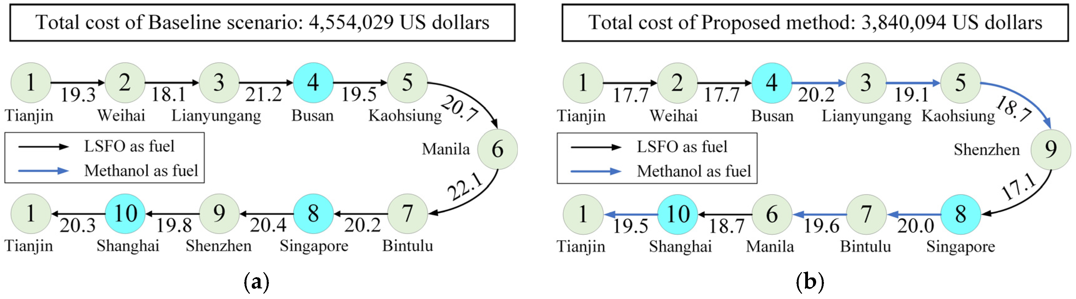
1	1000	3,840,094
2	1500	3,582,746

and Figure 8a,b.

As shown in Figure 8a, increasing the methanol tank capacity from 1000 tons to 1500 tons results in a further reduction in the total cost to 3,582,746 USD. This represents a significant decrease of 1,347,318 USD compared to the baseline scenario. Figure 8b demonstrates that increasing the methanol tank capacity also contributes to a further reduction in vessel emissions of CO₂, NOx, SOx, PM, and CO. This phenomenon primarily arises because expanding the methanol tank capacity enables the vessel to utilize LSFO, which, despite its higher cost, exhibits a higher emission factor. Furthermore, it can be inferred that under the carbon trading policy, the optimized voyage decision-making strategy yields a carbon emission reduction advantage of 195,058 USD compared to the baseline scenario without optimized routes and speeds. If the methanol fuel tank capacity is increased to 1500 tons, this carbon reduction benefit can be further enhanced to 222,613 USD.

7. Conclusions

With increasingly stringent emission regulations, the use of conventional fuels will face greater restrictions, leading to a growing market share for methanol dual-fuel vessels. This trend is already shaping the shipbuilding industry. Although methanol may be more expensive than traditional fuels, strict emission reduction policies will incentivize ship operators to opt for methanol over conventional options. Consequently, developing a joint optimization algorithm for route and speed planning tailored to methanol dual-fuel vessels holds significant practical importance.

In conclusion, this study addresses the critical need for optimizing route and speed decisions for methanol dual-fuel-powered ships, a novel and environmentally friendly vessel type. By developing a mixed-integer nonlinear programming (MINLP) model aimed at minimizing operating costs and emissions and proposing an improved genetic algorithm (GA) integrated with the Nonlinear Programming Branch-and-Bound (NLP-BB) method, we have demonstrated significant advancements over conventional optimization strategies. The case study results reveal that the proposed approach reduces operating costs by more than 15% and effectively decreases emissions of CO₂, NOx, SOx, PM, and CO. Comparative experiments further validate the computational efficiency of our algorithm, which outperforms both the traditional GA and the LINGO solver. The sensitivity analysis highlights the impact of the methanol tank capacity on cost and emission reductions, suggesting that larger tank capacities can further enhance the benefits of methanol as a marine fuel. Overall, this research provides a robust framework for the operational optimization of methanol dual-fuel ships, contributing to the maritime industry’s transition towards sustainable and cost-effective energy solutions.

The primary contribution of this article lies in its exploration of the intriguing characteristics of methanol dual-fuel vessels. Specifically, due to the price disparity between methanol and conventional fuel, the optimal route and speed decision strategies for dual-fuel vessels capable of freely switching between methanol and traditional fuel will differ. This implies that the route and speed plans designed for conventional fuel vessels are no longer applicable to methanol dual-fuel vessels, offering valuable insights for shipping companies. The proposed model and solution algorithm in this study can also be adapted and applied to other alternative energy sources, such as ammonia or hydrogen.

Moreover, this study does not account for the impact of fuel price fluctuations on the results. Future research should explore scenarios involving uncertainties in bunkering fuel prices at ports and further incorporate refueling strategies as a decision variable.

References

- IMO 2020—Cutting Sulphur Oxide Emissions. Available online: https://www.imo.org/en/MediaCentre/HotTopics/Pages/Sulphur-2020.aspx (accessed on 6 June 2024).
- IMO. Historic Background—IMO GHG Studies. 2021. Available online: https://www.imo.org/en/OurWork/Environment/Pages/Historic%20Background%20GHG.aspx (accessed on 27 September 2024).
- IMO. Marine Environment Protection Committee (MEPC), 63rd Session, 27 February to 2 March. 2012. Available online: https://www.imo.org/en/MediaCentre/MeetingSummaries/Pages/MEPC-63rd-session.aspx (accessed on 27 September 2024).
- REUTERS. EU Proposes Adding Shipping to Its Carbon Trading Market. 2021. Available online: https://www.reuters.com/business/sustainable-business/eu-proposes-adding-shipping-its-carbon-trading-market-2021-07-14/ (accessed on 27 September 2024).
- Wu, M. Carbon Emission Trading Scheme in the shipping sector: Drivers, challenges, and impacts. Mar. Policy 2022, 138, 104989. [Google Scholar]
- Brynolf, S.; Fridell, E.; Andersson, K. Environmental assessment of marine fuels: Liquefied natural gas, liquefied biogas, methanol and bio-methanol. J. Clean. Prod. 2014, 74, 86–95. [Google Scholar]
- Bilgili, L. A systematic review on the acceptance of alternative marine fuels. Renew. Sustain. Energy Rev. 2023, 182, 113367. [Google Scholar] [CrossRef]
- Hansson, J.; Månsson, S.; Brynolf, S.; Grahn, M. Alternative marine fuels: Prospects based on multi-criteria decision analysis involving Swedish stakeholders. Biomass Bioenergy 2019, 126, 159–173. [Google Scholar]
- Xing, H.; Stuart, C.; Spence, S.; Chen, H. Alternative fuel options for low carbon maritime transportation: Pathways to 2050. J. Clean. Prod. 2021, 297, 126651. [Google Scholar]
- Strazza, C.; Del Borghi, A.; Costamagna, P.; Traverso, A.; Santin, M.J.A.E. Comparative LCA of methanol-fuelled SOFCs as auxiliary power systems on-board ships. Appl. Energy 2010, 87, 1670–1678. [Google Scholar]
- McKinlay, C.J.; Turnock, S.R.; Hudson, D.A. Route to zero emission shipping: Hydrogen, ammonia or methanol? Int. J. Hydrogen Energy 2021, 46, 28282–28297. [Google Scholar]
- Rouwenhorst, K.H.R.; Van der Ham, A.G.; Mul, G.; Kersten, S.R. Islanded ammonia power systems: Technology review & conceptual process design. Renew. Sustain. Energy Rev. 2019, 114, 109339. [Google Scholar]
- Parris, D.; Spinthiropoulos, K.; Ragazou, K.; Giovou, A.; Tsanaktsidis, C. Methanol, a Plugin Marine Fuel for Green House Gas Reduction—A Review. Energies 2024, 17, 605. [Google Scholar] [CrossRef]
- Clarksons Research. Shipping Review Outlook; Clarkson Research Services: Ledbury, UK, 2023. [Google Scholar]
- Gao, T.; Tian, J.; Liu, C.; Huang, C.; Wu, H.; Yuan, Z. A model for speed and fuel refueling strategy of methanol dual-fuel liners with emission control areas. Transp. Policy 2025, 161, 1–16. [Google Scholar]
- Ronen, D. The effect of oil price on containership speed and fleet size. J. Oper. Res. Soc. 2011, 62, 211–216. [Google Scholar]
- Zhang, J.; Yang, T.; Ma, W. Ship speed optimization based on multi-objective particle swarm algorithm. J. Syst. Simul. 2019, 31, 787–794. [Google Scholar]
- Tzortzis, G.; Sakalis, G. A dynamic ship speed optimization method with time horizon segmentation. Ocean Eng. 2021, 226, 108840. [Google Scholar]
- Hua, R.; Yin, J.; Wang, S.; Han, Y.; Wang, X. Speed optimization for maximizing the ship’s economic benefits considering the Carbon Intensity Indicator (CII). Ocean Eng. 2024, 293, 116712. [Google Scholar]
- Luo, X.; Yan, R.; Wang, S. Ship sailing speed optimization considering dynamic meteorological conditions. Transp. Res. Part C Emerg. Technol. 2024, 167, 104827. [Google Scholar] [CrossRef]
- Marashian, A.; Böling, J.M.; Razminia, A.; Hyvönen, J.; Vettor, R.; Gustafsson, W.; Pirttikangas, M.; Björkqvist, J. Combined engine conFiguration and speed optimization for fuel savings on cruise ships. Ocean Eng. 2025, 322, 120387. [Google Scholar]
- Huotari, J.; Manderbacka, T.; Ritari, A.; Tammi, K. Convex optimisation model for ship speed profile: Optimisation under fixed schedule. J. Mar. Sci. Eng. 2021, 9, 730. [Google Scholar] [CrossRef]
- Zincir, B. Slow steaming application for short-sea shipping to comply with the CII regulation. Brodogr. Int. J. Nav. Archit. Ocean Eng. Res. Dev. 2023, 74, 21–38. [Google Scholar]
- Taskar, B.; Sasmal, K.; Yiew, L.J. A case study for the assessment of fuel savings using speed optimization. Ocean Eng. 2023, 274, 113990. [Google Scholar]
- Luo, X.; Yan, R.; Wang, S. Comparison of deterministic and ensemble weather forecasts on ship sailing speed optimization. Transp. Res. Part D Transp. Environ. 2023, 121, 103801. [Google Scholar]
- Li, X.; Sun, B.; Jin, J.; Ding, J. Ship speed optimization method combining Fisher optimal segmentation principle. Appl. Ocean Res. 2023, 140, 103743. [Google Scholar] [CrossRef]
- Tsou, M.-C. Integration of a geographic information system and evolutionary computation for automatic routing in coastal navigation. J. Navig. 2010, 63, 323–341. [Google Scholar] [CrossRef]
- Szlapczynska, J.; Szlapczynski, R. Preference-based evolutionary multi-objective optimization in ship weather routing. Appl. Soft Comput. 2019, 84, 105742. [Google Scholar] [CrossRef]
- Wei, S.; Zhou, P. 23. Development of a 3D Dynamic Programming Method for Weather Routing. In Methods and Algorithms in Navigation: Marine Navigation and Safety of Sea Transportation; CRC Press: Boca Raton, FL, USA, 2011; p. 181. [Google Scholar]
- Chang, Y.-C.; Tseng, R.S.; Chen, G.Y.; Chu, P.C.; Shen, Y.T. Ship routing utilizing strong ocean currents. J. Navig. 2013, 66, 825–835. [Google Scholar] [CrossRef]
- Ma, W.; Han, Y.; Tang, H.; Ma, D.; Zheng, H.; Zhang, Y. Ship route planning based on intelligent mapping swarm optimization. Comput. Ind. Eng. 2023, 176, 108920. [Google Scholar] [CrossRef]
- Wei, Z.; Zhao, L.; Zhang, X.; Lv, W. Jointly optimizing ocean shipping routes and sailing speed while considering involuntary and voluntary speed loss. Ocean Eng. 2022, 245, 110460. [Google Scholar] [CrossRef]
- Cheng, L.; Xu, L.; Bai, X. Cargo selection, route planning, and speed optimization in tramp shipping under carbon intensity indicator (CII) regulations. Transp. Res. Part E Logist. Transp. Rev. 2025, 194, 103948. [Google Scholar] [CrossRef]
- Lashgari, M.; Akbari, A.A.; Nasersarraf, S. A new model for simultaneously optimizing ship route, sailing speed, and fuel consumption in a shipping problem under different price scenarios. Appl. Ocean Res. 2021, 113, 102725. [Google Scholar] [CrossRef]
- Ma, D.; Ma, W.; Jin, S.; Ma, X. Method for simultaneously optimizing ship route and speed with emission control areas. Ocean Eng. 2020, 202, 107170. [Google Scholar] [CrossRef]
- Ma, W.; Lu, T.; Ma, D.; Wang, D.; Qu, F. Ship route and speed multi-objective optimization considering weather conditions and emission control area regulations. Marit. Policy Manag. 2021, 48, 1053–1068. [Google Scholar] [CrossRef]
- Ma, W.; Ma, D.; Ma, Y.; Zhang, J.; Wang, D. Green maritime: A routing and speed multi-objective optimization strategy. J. Clean. Prod. 2021, 305, 127179. [Google Scholar]
- Ma, D.; Ma, W.; Hao, S.; Jin, S.; Qu, F. Ship’s response to low-sulfur regulations: From the perspective of route, speed and refueling strategy. Comput. Ind. Eng. 2021, 155, 107140. [Google Scholar]
- Zhen, L.; Hu, Z.; Yan, R.; Zhuge, D.; Wang, S. Route and speed optimization for liner ships under emission control policies. Transp. Res. Part C Emerg. Technol. 2020, 110, 330–345. [Google Scholar] [CrossRef]
- Wan, S.; Li, S.; Chen, Z.; Tang, Y. An ultrasonic-AI hybrid approach for predicting void defects in concrete-filled steel tubes via enhanced XGBoost with Bayesian optimization. Case Stud. Constr. Mater. 2025, 22, e04359. [Google Scholar] [CrossRef]
- Nong, Y.; Chen, Z.; Chen, Y.; Tang, Y.; Wang, Y.; Liu, K.; Qin, M. Molecular insights into the effect of adsorption and reaction of H2O-O2-Cl- on initial electrochemical corrosion of steel. Electrochim. Acta 2025, 511, 145385. [Google Scholar] [CrossRef]
- Zhang, D.; Liu, W.; Fu, K.; Wang, F.; Wu, X.; Zhao, C.; Shen, C.; Yu, Z.; Tang, Y. Analytical Model and Optimization of Joint Systems in Modular Precast Foundations for Onshore Wind Turbines. Buildings 2024, 14, 3952. [Google Scholar] [CrossRef]
- Omer, M.; Lijie, G.; Yunchao, T.; Okasha, N.M.; Azimi, S.J.; Namdar, A.; Azhar, F. The displacement mechanism of the cracked rock—A seismic design and prediction study using XFEM and ANNs. Adv. Model. Simul. Eng. Sci. 2024, 11, 4. [Google Scholar]
- Tan, R.; Duru, O.; Thepsithar, P. Assessment of relative fuel cost for dual fuel marine engines along major Asian container shipping routes. Transp. Res. Part E Logist. Transp. Rev. 2020, 140, 102004. [Google Scholar] [CrossRef]
- He, P.; Jin, J.G.; Pan, W.; Chen, J. Route, speed, and bunkering optimization for LNG-fueled tramp ship with alternative bunkering ports. Ocean Eng. 2024, 305, 117957. [Google Scholar]
- Drozhzhyn, O.; Koskina, Y.; Tykhonina, I. “Liner shipping”: The evolution of the concept. Pomorstvo 2021, 35, 365–371. [Google Scholar]
- Raza, Z.; Woxenius, J.; Vural, C.A.; Lind, M. Digital transformation of maritime logistics: Exploring trends in the liner shipping segment. Comput. Ind. 2023, 145, 103811. [Google Scholar] [CrossRef]
- Sun, Y.; Zheng, J.; Yang, L.; Li, X. Allocation and trading schemes of the maritime emissions trading system: Liner shipping route choice and carbon emissions. Transp. Policy 2024, 148, 60–78. [Google Scholar] [CrossRef]
- Chen, J.; Ye, J.; Zhuang, C.; Qin, Q.; Shu, Y. Liner shipping alliance management: Overview and future research directions. Ocean Coast. Manag. 2022, 219, 106039. [Google Scholar]
- Ma, W.; Hao, S.; Ma, D.; Wang, D.; Jin, S.; Qu, F. Scheduling decision model of liner shipping considering emission control areas regulations. Appl. Ocean Res. 2021, 106, 102416. [Google Scholar]
- Wang, C.; Xu, C. Sailing speed optimization in voyage chartering ship considering different carbon emissions taxation. Comput. Ind. Eng. 2015, 89, 108–115. [Google Scholar]
- Drube, T.K.; Gerlach, J.M.; Leach, T.S.; Vogel, B.; Klebanoff, L.E. Exploring variations in the weight, size and shape of liquid hydrogen tanks for zero-emission fuel-cell vessels. Int. J. Hydrogen Energy 2024, 80, 1441–1465. [Google Scholar]
- Kronqvist, J.; Bernal, D.E.; Lundell, A.; Grossmann, I.E. A review and comparison of solvers for convex MINLP. Optim. Eng. 2019, 20, 397–455. [Google Scholar]
- Epelle, E.I.; Gerogiorgis, D.I. A computational performance comparison of MILP vs. MINLP formulations for oil production optimisation. Comput. Chem. Eng. 2020, 140, 106903. [Google Scholar]
- Mogale, D.G.; Kumar, S.K.; Tiwari, M.K. An MINLP model to support the movement and storage decisions of the Indian food grain supply chain. Control Eng. Pract. 2018, 70, 98–113. [Google Scholar] [CrossRef]
- Vladov, S. Cognitive Method for Synthesising a Fuzzy Controller Mathematical Model Using a Genetic Algorithm for Tuning. Big Data Cogn. Comput. 2025, 9, 17. [Google Scholar] [CrossRef]
- Tynchenko, V.; Lomazov, A.; Lomazov, V.; Evsyukov, D.; Nelyub, V.; Borodulin, A.; Gantimurov, A.; Malashin, I. Adaptive Management of Multi-Scenario Projects in Cybersecurity: Models and Algorithms for Decision-Making. Big Data Cogn. Comput. 2024, 8, 150. [Google Scholar] [CrossRef]
- Malashin, I.; Masich, I.; Tynchenko, V.; Nelyub, V.; Borodulin, A.; Gantimurov, A. Application of Natural Language Processing and Genetic Algorithm to Fine-Tune Hyperparameters of Classifiers for Economic Activities Analysis. Big Data Cogn. Comput. 2024, 8, 68. [Google Scholar] [CrossRef]
- Fleszar, K. A branch-and-bound algorithm for the quadratic multiple knapsack problem. Eur. J. Oper. Res. 2022, 298, 89–98. [Google Scholar] [CrossRef]
- Jiao, H.; Wang, W.; Shang, Y. Outer space branch-reduction-bound algorithm for solving generalized affine multiplicative problems. J. Comput. Appl. Math. 2023, 419, 114784. [Google Scholar] [CrossRef]
- Gupta, O.K.; Ravindran, A. Branch and bound experiments in convex nonlinear integer programming. Manag. Sci. 1985, 31, 1533–1546. [Google Scholar] [CrossRef]
- Bonami, P.; Biegler, L.T.; Conn, A.R.; Cornuéjols, G.; Grossmann, I.E.; Laird, C.D.; Lee, J.; Lodi, A.; Margot, F.; Sawaya, N.; et al. An algorithmic framework for convex mixed integer nonlinear programs. Discret. Optim. 2008, 5, 186–204. [Google Scholar] [CrossRef]
- Billionnet, A.; Elloumi, S.; Lambert, A. A branch and bound algorithm for general mixed-integer quadratic programs based on quadratic convex relaxation. J. Comb. Optim. 2014, 28, 376–399. [Google Scholar] [CrossRef]