1. Introduction
Walking is a fundamental aspect of human activity, relying on the seamless coordination of muscles, joints, and nerves. A deeper understanding of this process is crucial for identifying and managing gait abnormalities and musculoskeletal disorders [
1,
2,
3,
4,
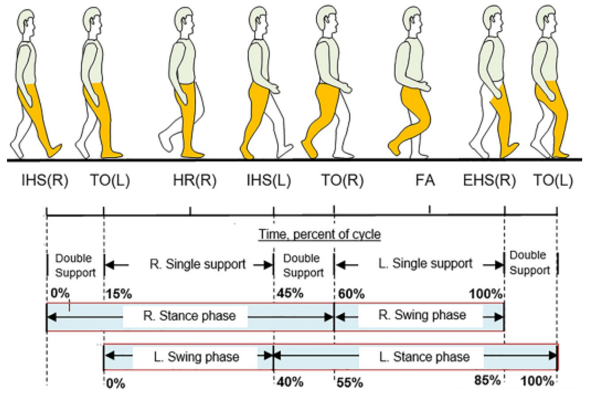
5]. Gait, which refers to the rhythmic movement of the legs during walking, varies among individuals based on age and health status. It is commonly divided into two main phases (see
Figure 1): the stance phase (0–60%) and the swing phase (60–100%).
Gait phase classification plays a vital role in clinical diagnostics, rehabilitation, and assistive technologies, as it enables precise monitoring of movement patterns and early detection of abnormalities. While traditional machine learning (ML) and deep learning (DL) approaches have significantly advanced gait analysis, challenges remain in accurately classifying multiple gait phases, optimizing feature selection, and improving model generalizability across diverse datasets. The primary objective of this study is to develop and benchmark ML models for quinary gait phase classification (five-phase classification) to enhance gait recognition accuracy and applicability. Specifically, this study investigates the impact of different preprocessing techniques, feature scaling methods, and training methodologies to optimize classification performance. The findings of this study aim to bridge the gap between research and real-world applications, with potential benefits for gait rehabilitation, intelligent orthotic devices, and fall prevention systems.
Recent advances in ML and DL have shown promising results in gait phase classification, with various studies exploring different approaches to improve classification accuracy. Park et al. [
7] investigated binary (stance/swing) and ternary (weight acceptance/single limb support/limb advancement) gait phase classification using four ML algorithms: Decision Tree (DT),
k-Nearest Neighbors (
k-NNs), Support Vector Machine (SVM), and Neural Network (NN). Their findings demonstrated that SVM achieved the highest classification accuracy (93.44% for binary and 91.72% for ternary classification), with muscle synergy features outperforming traditional EMG features. These results highlight the potential of modular muscle coordination in enhancing gait phase detection for neurological rehabilitation and assistive devices. Zhang et al. [
8] proposed a multi-information fusion method integrating surface electromyography (sEMG) signals, knee joint angles, and plantar pressure data to improve classification accuracy. A modified CNN model was used for classification, achieving 98% accuracy and 92% F1-score under five-fold cross-validation. Results indicate multi-information fusion significantly outperforms single-source approaches, proving its effectiveness for real-time exoskeleton control. Similarly, Hwang et al. [
9] developed an IMU-based abnormal gait classification system using SVM, Random Forest (RF), and Extreme Gradient Boosting (XGB). Their model classified three gait types (normal, knee impairment, ankle impairment) with 91% accuracy using Recursive Feature Elimination with Cross-Validation (RFECV). Comparatively, a walkway-based system achieved only 77% accuracy, highlighting the superiority of IMU sensors for gait assessment. These findings suggest that IMU-based gait classification can enhance patient monitoring and rehabilitation strategies. In the context of intelligent orthotic devices, the authors of [
10] evaluated ML classifiers (J-48 DT, RF, Multi-Layer Perceptrons, and SVMs) for classifying gait phases using thigh-mounted inertial sensors. Data from 31 participants were analyzed with 5-fold and 10-fold cross-validation, where J-48 DT achieved 97.5% accuracy with knee angle input and 97.0% accuracy without it, suggesting thigh-mounted IMU sensors alone can provide robust classification for real-time orthosis control.
Furthermore, Jung et al. [
11] proposed an ML-based approach using IMU sensors to classify gait phases and estimate joint moments. Their model optimized feature selection, reducing joint angles from six to three, with only a 4.04% accuracy drop, and further reduction to two angles caused a 7.46% decrease. They extended their method using OpenSim for joint-moment regression, correlating gait phases with biomechanical forces. Their findings suggest efficient feature selection and robust gait classification, benefiting prosthetics, exoskeletons, and rehabilitation applications. Lastly, Mekni et al. [
12] investigated binary (stance/swing) and ternary (stance-I/stance-II/swing) gait phase classification using six ML algorithms, demonstrating that RF consistently outperformed other classifiers, achieving high accuracy. These studies collectively emphasize the growing impact of ML-driven gait phase classification in biomechanics, clinical diagnostics, rehabilitation, and assistive technologies, paving the way for enhanced real-time control of exoskeletons and intelligent orthotic devices. Further extending this work, Mekni et al. [
13] explored multi-class gait phase recognition by dividing the gait cycle into five distinct subphases, showing that RF remained the most effective classifier, while participant-based data partitioning contributed to improved robustness. Additionally, Mekni et al. [
14] analyzed the impact of varied training methods and feature selection, comparing classification performance using five and ten lower-body movement features. Their findings emphasized that increasing movement features enhanced classification accuracy across all ML models, with RF reaching the best accuracy, reaffirming its suitability for gait phase recognition. Previous works by [
12,
13,
14] primarily focused on binary- and ternary-class gait classification using traditional ML models. However, several aspects remain unexplored. First, extending classification to a higher number of gait phases, such as quinary classification, could enhance the granularity of gait analysis. Second, the impact of different data preprocessing techniques, including various scaling methods and dimensionality reduction approaches, has not been systematically evaluated. Furthermore, their work lacks an in-depth investigation into generalizability across diverse datasets, which is crucial for real-world clinical and rehabilitation applications. Addressing these limitations could lead to more robust and adaptive gait classification frameworks.
Deep learning (DL) techniques have demonstrated superior performance in gait phase classification, significantly advancing clinical diagnostics, rehabilitation, and assistive technologies. Unlike conventional machine learning (CML) approaches that rely on handcrafted features, DL methods automatically learn relevant patterns from raw data, improving classification accuracy. Similarly, Ma et al. [
15] utilized joint angular sensors to achieve real-time robustness with 88.71% accuracy, though lower than DL methods. These studies collectively underscore DL’s effectiveness in gait analysis, particularly hybrid models, while highlighting limitations concerning hardware dependency, computational cost, and interpretability in diverse clinical and real-world applications. Zhang et al. [
8] introduced a multi-information fusion method integrating surface electromyography (sEMG), knee joint angles, and plantar pressure data, where a modified Convolutional Neural Network (CNN) achieved 98% accuracy and a 92% F1-score, proving the efficacy of CNNs for real-time exoskeleton control. Xia et al. [
16] combined CNN and BiLSTM to achieve 95.09% accuracy through local and temporal feature extraction, despite increased hardware complexity due to reliance on inertial measurement units and plantar pressure sensors. Similarly, Zheng et al. [
17] compared five DL approaches (CNN, Long Short-Term Memory (LSTM), Gated Recurrent Unit (GRU), Bidirectional LSTM (BiLSTM), and Convolutional LSTM (ConvLSTM)) against four CML methods for age-related gait classification based on accelerometer data, demonstrating that DL consistently outperformed CML, with GRU attaining the highest accuracy (89.3%) and all DL models achieving AUC values above 0.94 compared to 0.83 for the best CML model. However, multiple sensor arrays increased hardware complexity and posed challenges for real-time processing. Zheng et al. [
18] further validated DL’s capability in age-related gait classification, achieving 81.4% accuracy (AUC = 0.89) with CNN on single-stride data, and 84.5% accuracy (AUC = 0.94) with GRU on multi-stride data, incorporating SHapley Additive exPlanations (SHAPs) to enhance interpretability by identifying influential features such as heel contact and toe-off accelerations.
Machine learning models have been widely applied to gait analysis, offering different strengths and limitations depending on their architecture. Traditional ML models, such as SVM, DT, and
k-NN, have demonstrated strong interpretability and require relatively small datasets but struggle with complex gait dynamics. In contrast, DL models like CNN and RNN have outperformed traditional classifiers in recognizing abnormal gait patterns but require extensive labeled data and high computational resources [
2,
19,
20]. CNNs, for example, have been particularly effective in feature extraction from time-series gait data [
19]. However, recurrent models, such as LSTM networks, offer advantages in capturing temporal dependencies but may suffer from overfitting when applied to small datasets [
4]. Given these trade-offs, recent research has focused on optimizing feature selection and training methodologies to maximize accuracy while improving model efficiency. Summarizing the limitations of existing models, three major challenges can be observed. First, generalizability remains a concern, as many models are trained on small, homogeneous datasets, resulting in poor performance on unseen subjects. Second, prior studies have not systematically evaluated the impact of feature selection techniques and preprocessing methods, such as PCA, on classification performance. Lastly, training strategies have largely relied on traditional random sampling without a thorough comparison to participant-based splitting, which can significantly affect model robustness. Addressing these challenges could enhance the reliability and applicability of gait classification models in real-world settings. This study systematically benchmarks multiple ML models for quinary gait phase classification to address these gaps, investigating the effects of different preprocessing techniques and training methodologies. In the five-subphase analysis, RF demonstrated strong performance, achieving an accuracy of 94.95%, an RMSE of 0.4461, and an
score of 90.09% across all scaling methods. Notably, this accuracy surpasses prior studies that focused on binary (stance/swing) or ternary (stance-I/stance-II/swing) gait phase classification, where reported accuracy rates typically ranged between 85% and 93% [
12,
13]. This improvement highlights the advantages of adopting a more granular quinary classification approach and optimizing ML training methodologies, ultimately enhancing gait phase recognition accuracy and clinical applicability. Building on these advancements, the main contributions of this work are as follows:
- (i)
Unlike conventional studies that classify gait into two or three phases, this work extends the analysis to a five-phase classification, providing a more detailed understanding of gait mechanics.
- (ii)
This study evaluates two training methodologies—stratified random sampling and participant-based splitting—to analyze inter-individual variability and improve model robustness. Such a comparison between the outcome effects of two training methodologies has hardly been explored in the literature.
- (iii)
The research systematically investigates two feature scaling techniques—Min–Max Scaling (MMS) and Standard Scaling (SS)—as well as Principal Component Analysis (PCA), a dimensionality reduction method, to assess their impact on model performance.
- (iv)
Multiple ML algorithms, including k-NN, LR, DT, RF, SVM, NB, LDA, and QDA, are rigorously tested using metrics like accuracy, MSE, RMSE, and , benchmarking the most effective models for gait phase classification.
- (v)
This study’s findings provide practical implications for real-time gait monitoring, rehabilitation, and biomechanical analysis, enabling the development of efficient gait classification models applicable in clinical and robotics applications.
Aligned with these objectives, this study emphasizes the real-world applications of gait phase classification, bridging the gap between theoretical research and practical implementations in healthcare, assistive technology, and sports performance. Some of the key applications are outlined below.
Real-time gait monitoring: The proposed machine learning models can be integrated into wearable sensor systems to continuously track gait patterns, allowing for early detection of abnormalities and real-time feedback for users.
Rehabilitation and clinical applications: The classification models can assist clinicians in monitoring patients with neurological disorders, such as Parkinson’s disease or stroke, and evaluating the effectiveness of rehabilitation therapies based on gait phase recognition.
Intelligent prosthetics and robotics: The study provides insights into gait phase transitions, which can be utilized to enhance the control algorithms of robotic exoskeletons and intelligent prosthetic limbs, improving mobility for individuals with motor impairments.
Fall prevention systems: By accurately classifying gait phases, these models can contribute to predictive systems that assess gait stability and issue alerts for individuals at high risk of falls, particularly among elderly or mobility-impaired populations.
Sports and performance analysis: Athletes and sports professionals can use gait analysis models to optimize performance and reduce injury risks through personalized training adjustments based on biomechanical insights.
The structure of this paper is organized as follows:
Section 2 describes the methodology, including dataset details, ML algorithms, and hyperparameter selection.
Section 3 presents numerical results from the classification experiments.
Section 4 evaluates the performance of the models using various metrics.
Section 5 provides a discussion, and
Section 6 provides a comparative analysis of the results. Finally,
Section 7 concludes the study and outlines future research directions.
2. Dataset Involved
We used an existing dataset that includes 100 healthy adults aged between 21 and 79 years, ensuring a balanced representation across different age groups and genders. The dataset provides demographic information such as age, gender, height, and weight, offering insights into variations in gait. It also includes comprehensive biomechanical, kinematic, and kinetic data collected under different walking conditions. Each participant was assigned a unique identifier to preserve the anonymity and integrity of the data. For further details about the dataset, refer to the work of Bahadori et al. [
21,
22], and access it at
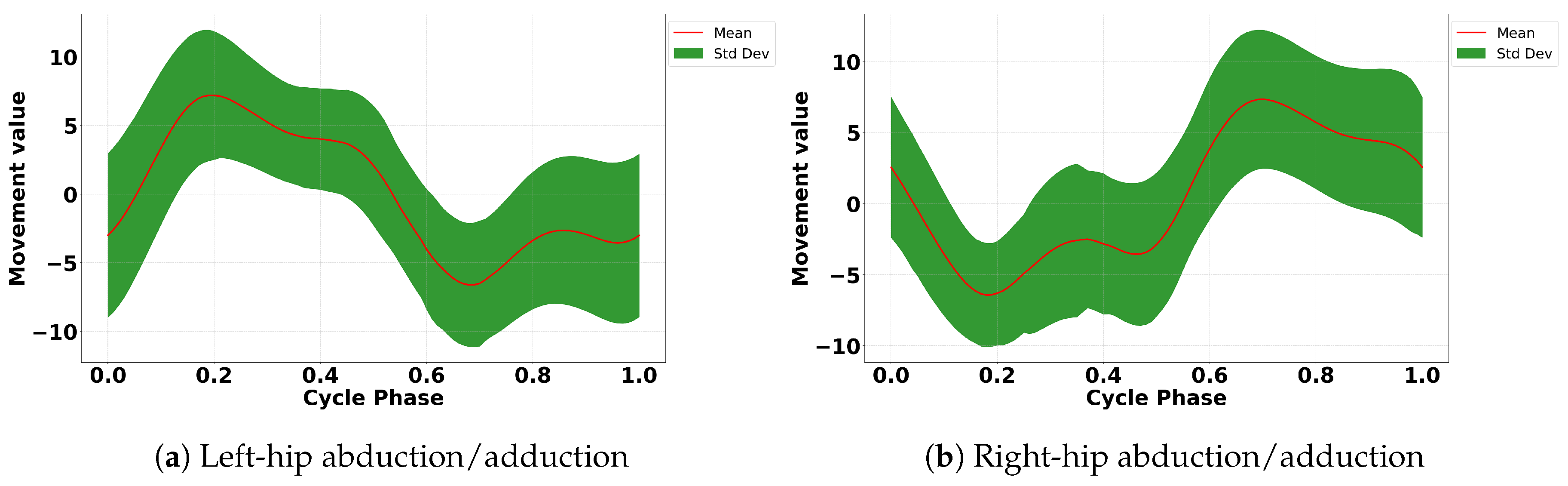
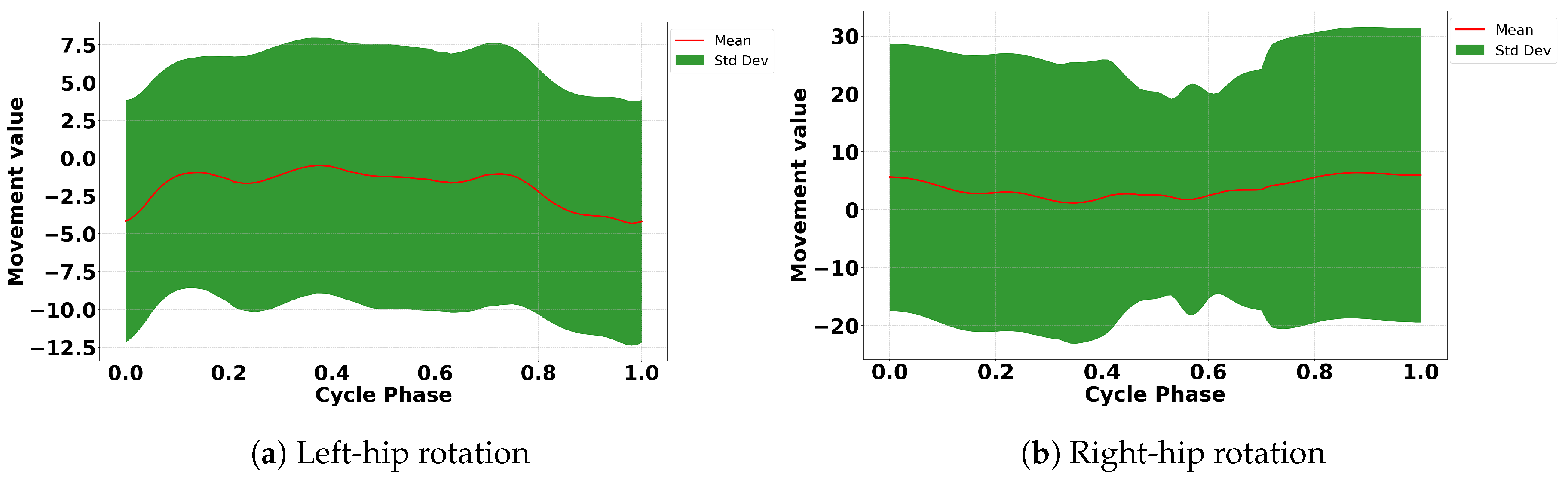
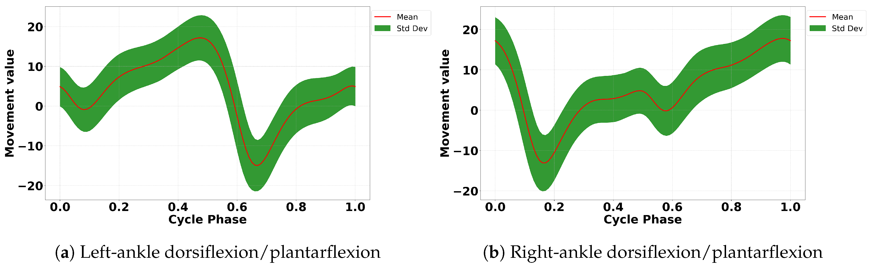
https://data.mendeley.com/datasets/wwnvw28n2m/1, accessed on 10 December 2024. Our study focused on analyzing specific lower-body movements, including ten key motions for both limbs such as hip flexion/extension, hip abduction/adduction, hip inter/intra rotation, knee flexion/extension, and ankle dorsiflexion/plantarflexion, as shown in
Figure 2,
Figure 3,
Figure 4,
Figure 5 and
Figure 6.
Table 1 presents a summary of the average anthropometric characteristics, including height, weight, and lower limb segment lengths, for both males and females.
To enhance the transparency and reproducibility of this study, we provide additional details on the data collection process and sample selection criteria. The dataset was obtained through controlled laboratory experiments using high-speed motion capture systems synchronized with force-instrumented treadmills. Each participant underwent a standardized gait assessment protocol, ensuring consistency in data acquisition. Strict inclusion criteria were applied, selecting only healthy adults without known musculoskeletal or neurological disorders, while individuals with gait impairments or recent lower-limb injuries were excluded. Participants represented a diverse distribution across age groups and genders to improve generalizability. Data preprocessing involved multiple steps, including outlier removal, missing value imputation, and normalization based on anthropometric parameters to enhance comparability. Additionally, motion cycle segmentation was performed to align gait events across participants, ensuring a robust dataset for biomechanical and ML analyses. These methodological refinements guarantee high-quality data, facilitating accurate modeling and reproducible research outcomes.
Data preprocessing is a critical phase in the analysis pipeline, ensuring the quality and reliability of data for accurate modeling. The raw motion data, collected from multiple participants and encompassing numerous motion cycles per individual, underwent several key steps to enhance its usability. First, data were cleaned to handle missing values, remove outliers, and correct inconsistencies, eliminating noise and inaccuracies that could impact the analysis. Next, the cleaned data were restructured to organize each participant’s 100 motion cycles into a standardized format, simplifying manipulation and feature extraction. Following this, relevant features related to the movement were selected, prioritizing data elements that contribute most significantly to accurate modeling while discarding irrelevant or redundant features. These comprehensive preprocessing steps ensured the dataset was clean, well organized, and optimized for robust analysis and modeling performance [
23,
24,
25].
4. Adopted Machine Learning Techniques
To ensure a robust and comprehensive gait classification, we selected a diverse set of ML algorithms, each with distinct advantages. The k-NNs algorithm was chosen for its simplicity and effectiveness in handling non-linear decision boundaries, making it suitable for gait patterns with subtle variations. LR, as a probabilistic classifier, provides interpretable predictions and works well for linearly separable data. DT and RF were included due to their capability to model complex decision boundaries while handling high-dimensional data efficiently. RF, as an ensemble method, further enhances prediction accuracy and reduces overfitting by aggregating multiple DTs. SVM was employed for its strong theoretical foundation in maximizing class separation through hyperplane optimization, which is particularly effective when gait features exhibit clear distinctions. NB, leveraging the probabilistic framework, offers fast and efficient classification, especially for datasets with independent features. LDA and QDA were chosen for their ability to project gait data into lower-dimensional spaces while maintaining class separability. LDA assumes a shared covariance structure across classes, making it useful when feature distributions follow Gaussian assumptions, whereas QDA allows for individual class covariance matrices, enabling greater flexibility in capturing complex gait variations. Each of these models was selected based on their ability to handle the multi-faceted nature of gait classification, balancing interpretability, computational efficiency, and predictive performance. Their strengths and limitations were carefully considered to ensure a well-rounded analysis of gait patterns in our study.
In classification models, training datasets serve as the foundation for constructing ML models capable of categorizing or classifying new samples [
29,
34]. Following this approach, we curated training and testing datasets and employed a variety of classification algorithms (
k-NN, LR, DT, RF, SVM, NB, LDA, QDA). These carefully selected algorithms played a crucial role in accurately classifying the stages of walking in our study, utilizing insights from the dataset to generate accurate predictions and enhance our comprehension of walking patterns [
35].
4.1. k-Nearest Neighbors (k-NNs)
The k-NNs algorithm classifies a sample by identifying the majority class among its k-Nearest Neighbors in the feature space. This non-parametric method relies entirely on the proximity of data points, determined by a chosen distance metric such as Euclidean, Manhattan, or Minkowski distance. The algorithm operates by calculating the distance between the sample and all training points, selecting the k closest points, and assigning the class that occurs most frequently among these neighbors. The prediction is determined by the majority vote of these k-Nearest Neighbors, making k-NN a straightforward and intuitive approach to classification tasks.
4.2. Logistic Regression (LR)
LR predicts the probability of a binary outcome using a logistic function. The mathematical formula is given as follows:
where
and
are the intercept and slope, respectively.
4.3. Decision Tree (DT)
The DT algorithm uses a hierarchical structure where nodes represent features and branches represent values. Based on the input’s feature value, the tree splits at each node until a leaf node is reached, assigning the sample to a class. The splitting logic can be represented as follows:
4.4. Random Forest (RF)
RF improves classification accuracy by aggregating predictions from multiple DTs. This ensemble method reduces overfitting and ensures robustness. The final prediction is computed as follows:
where
N is the number of DTs.
4.5. Support Vector Machine (SVM)
SVM constructs a hyperplane that separates the data into distinct classes with maximum margin. The decision boundary is defined by the following equation:
where
w represents the weight vector,
x is the input, and
c is the bias term.
4.6. Naive Bayes (NB)
NB is a probabilistic classifier based on Bayes’ theorem. It assumes independence among features and calculates the posterior probability of a class
z as follows:
where
is the prior probability and
is the likelihood of feature
given class
z.
4.7. Linear Discriminant Analysis (LDA)
LDA projects input data onto a lower-dimensional space to maximize class separability. It assumes that classes share the same covariance matrix. The formula for the projection is
where
is the projection matrix that maximizes the between-class variance.
4.8. Quadratic Discriminant Analysis (QDA)
QDA extends LDA by allowing each class to have its own covariance matrix. The decision function for QDA is given by
where
is the covariance matrix of class
k,
is the mean vector, and
is the prior probability of class
k.
5. Results and Discussions: A Comparative Analysis
The following analysis compares the performance of various ML models across different scaling techniques (MMS, SS, and PCA) using both the first and second approaches. The key metrics considered include CV score, MSE, RMSE, accuracy, and the
score, as listed in
Table 2,
Table 3,
Table 4,
Table 5,
Table 6 and
Table 7.
In the first approach of MMS, RF demonstrated the best overall performance with the highest accuracy of 94.95%, an RMSE of 0.4461, and a strong ability to explain data variability with the highest score of 90.09%, indicating its superior predictive power. On the other hand, k-NNs also performed well with an accuracy of 93.51%, but RF outshined it in terms of minimizing prediction error. In the second approach of MMS, SVM achieved the best results, with the highest accuracy of 90.04%, and the lowest RMSE of 0.8590, making it the top-performing model in this approach. LR also performed competitively, with an accuracy of 89.64% and the highest score of 62.00%, showing its ability to explain variability effectively.
For the first approach of SS, RF again outperformed other models with the highest accuracy of 94.90%, the lowest RMSE of 0.4549, and a strong score of 89.70%, highlighting its robust predictive performance. SVM was close behind, with an accuracy of 93.56% and competitive RMSE. In the second approach of SS, SVM took the lead with the highest accuracy of 90.24% and the lowest RMSE of 0.8465%, making it the best performer. LR followed closely with an accuracy of 90.04% and the highest score of 64.29%, showing its ability to handle variability effectively.
With PCA, RF performed the best in the first approach, with an accuracy of 94.95%, the lowest RMSE of 0.4377, and a solid score of 90.46%. SVM followed closely in the second approach, achieving the highest accuracy of 89.89% and the lowest RMSE of 0.8685%, while LR maintained the highest score of 65.79%, demonstrating strong performance in explaining variance.
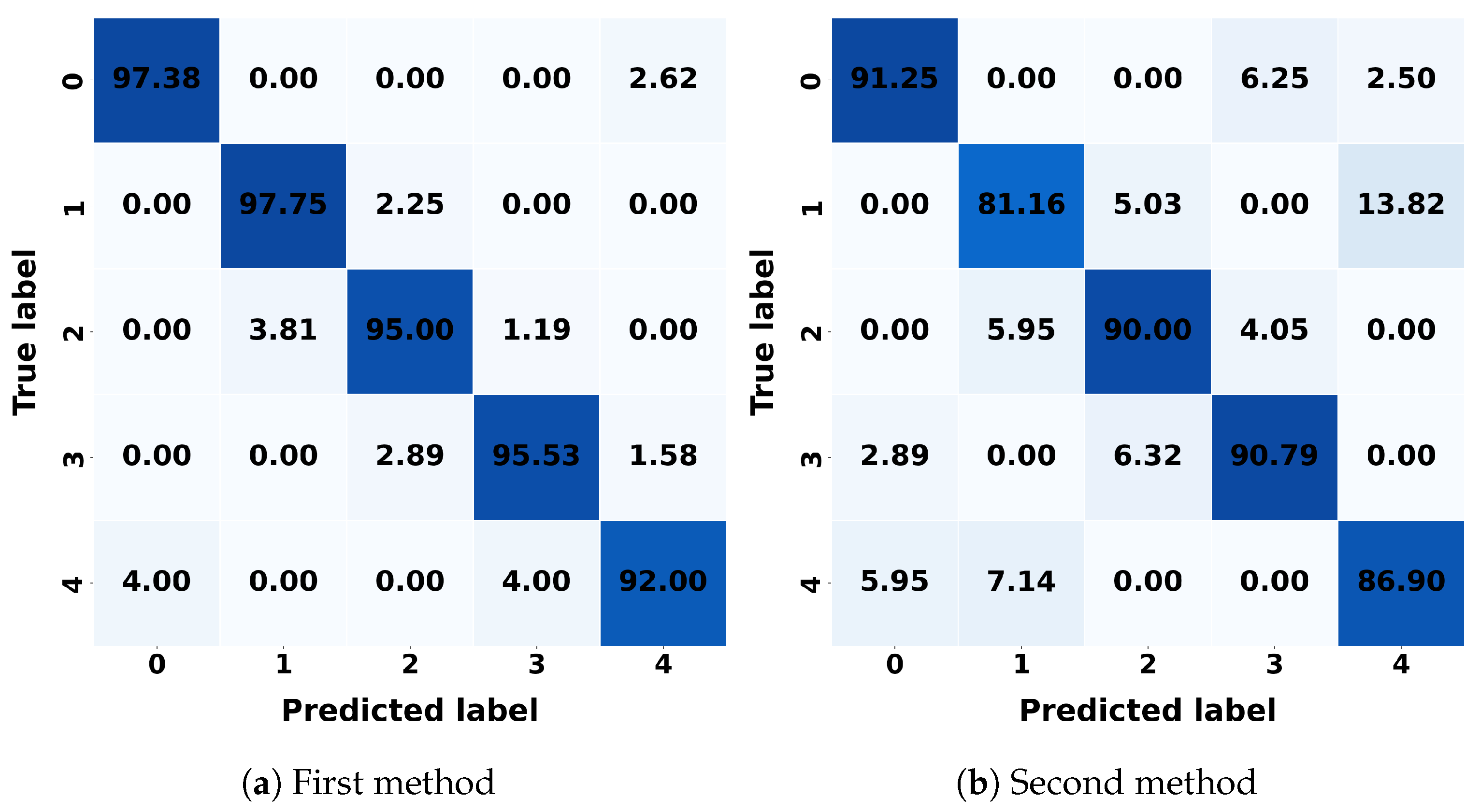
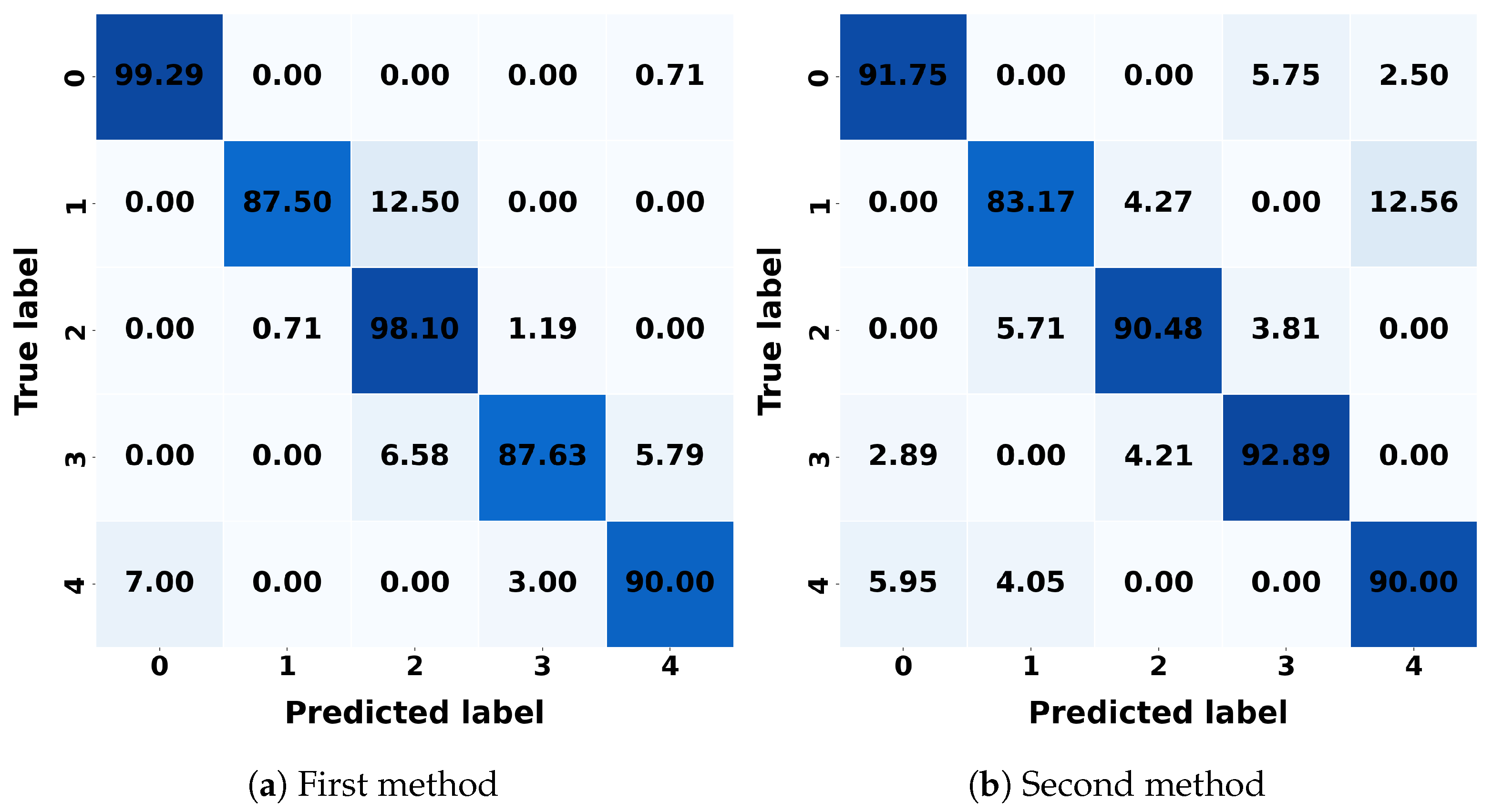
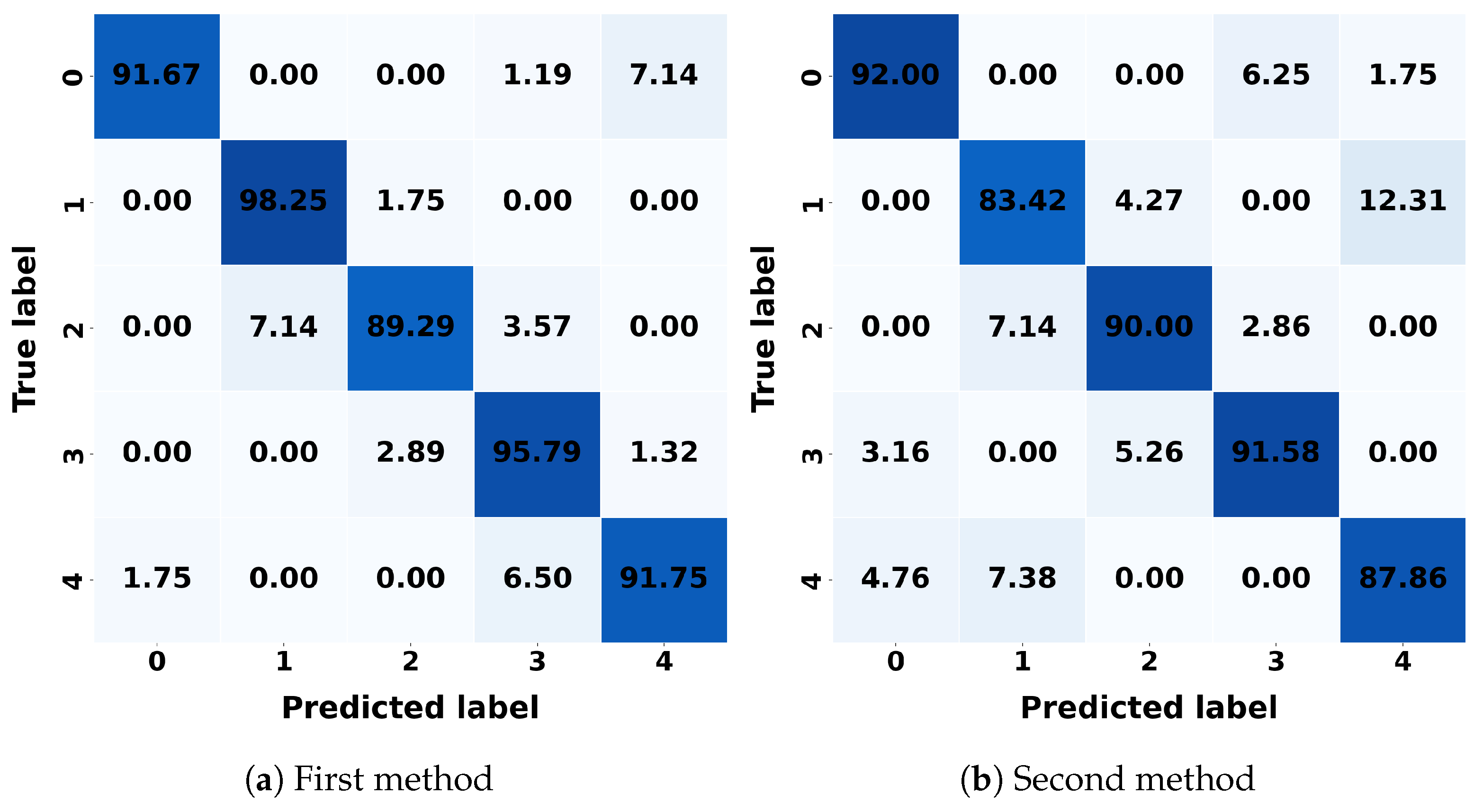
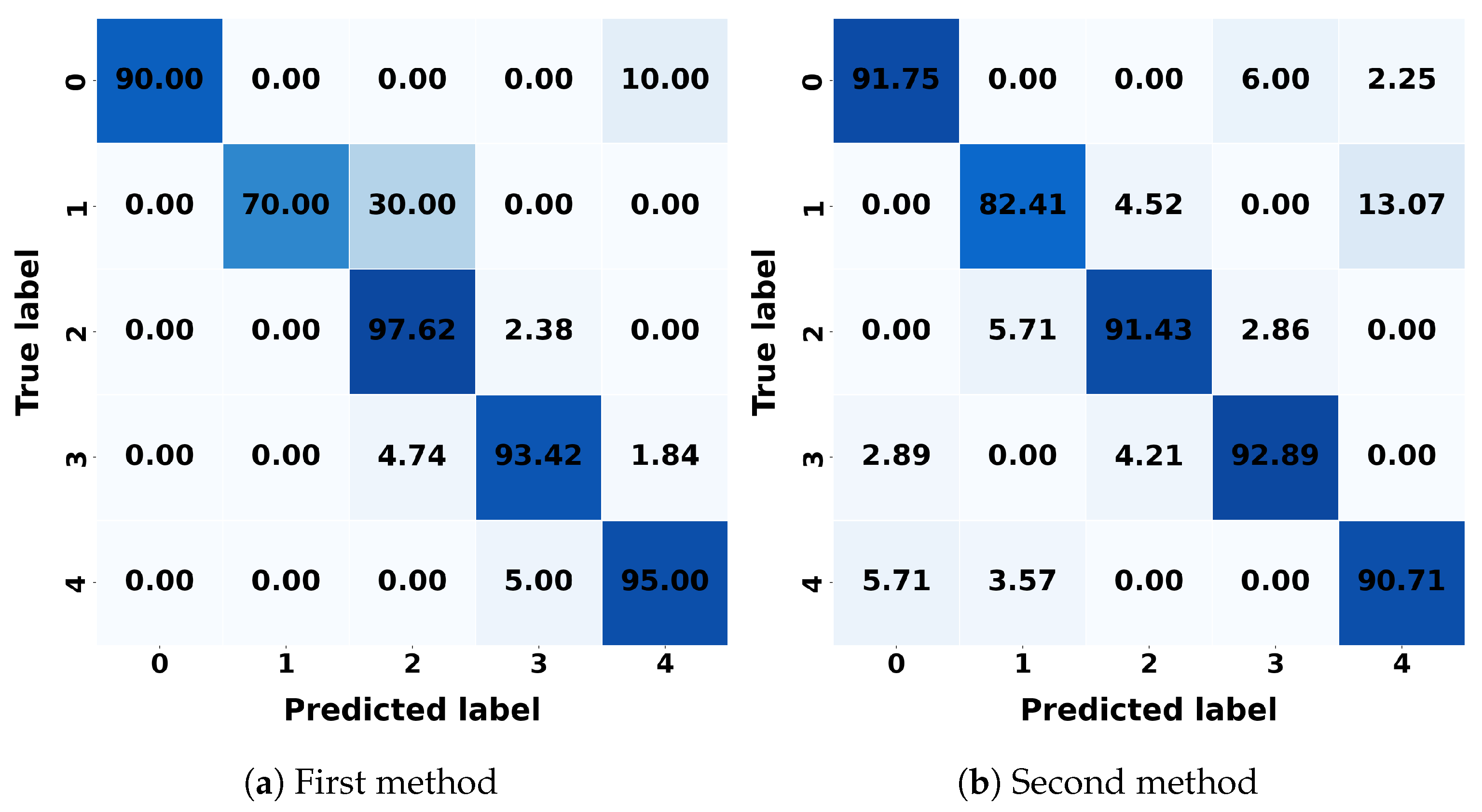
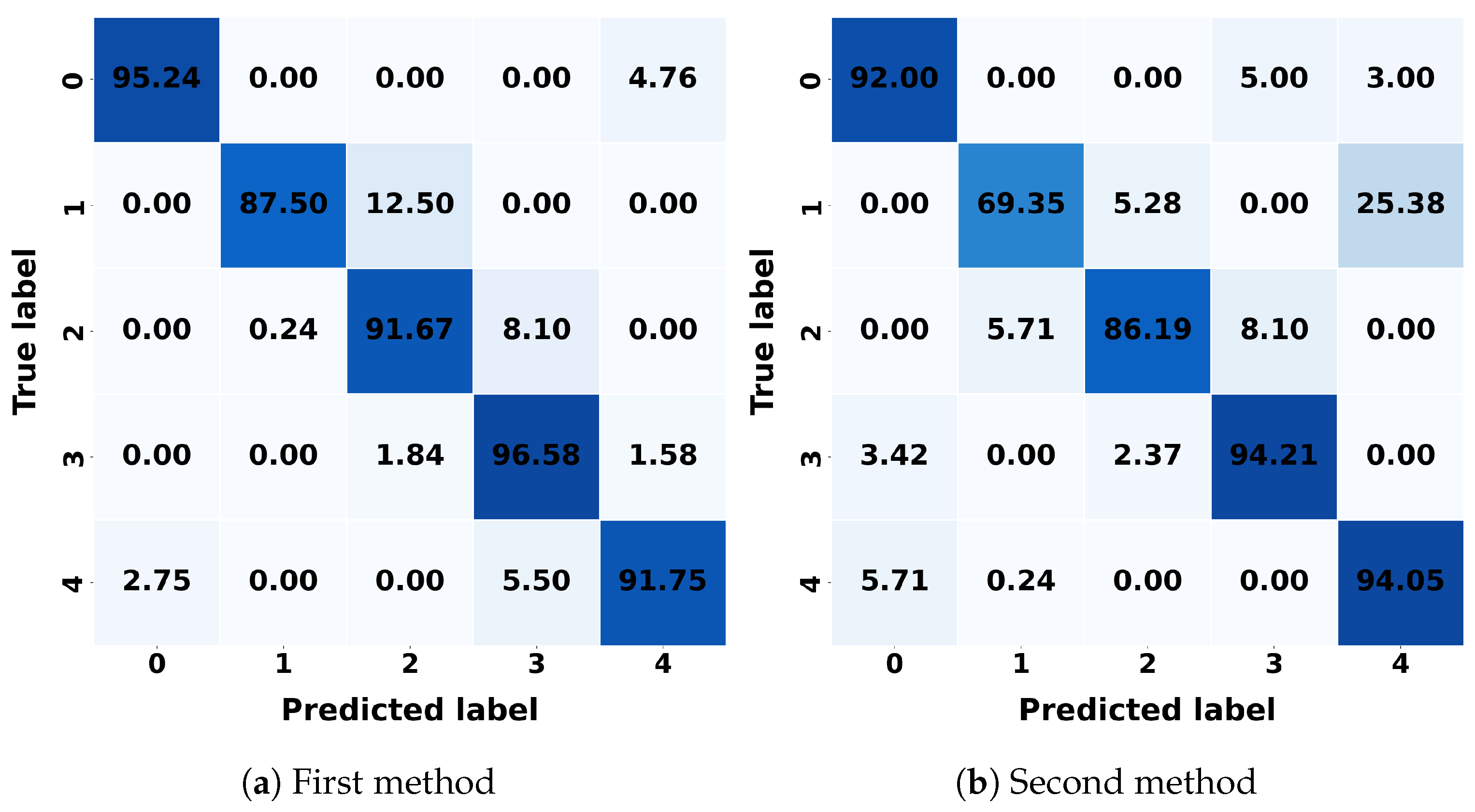
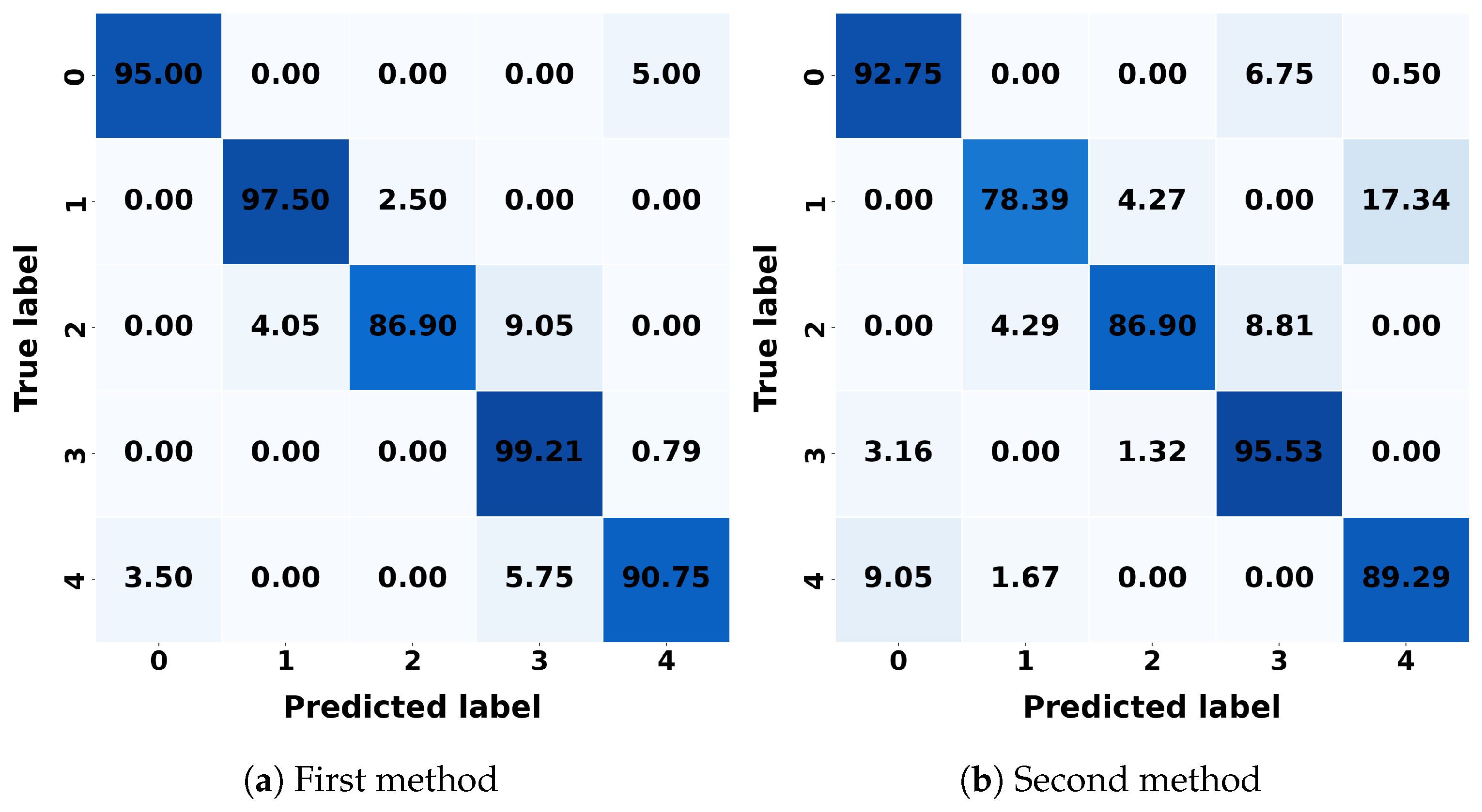
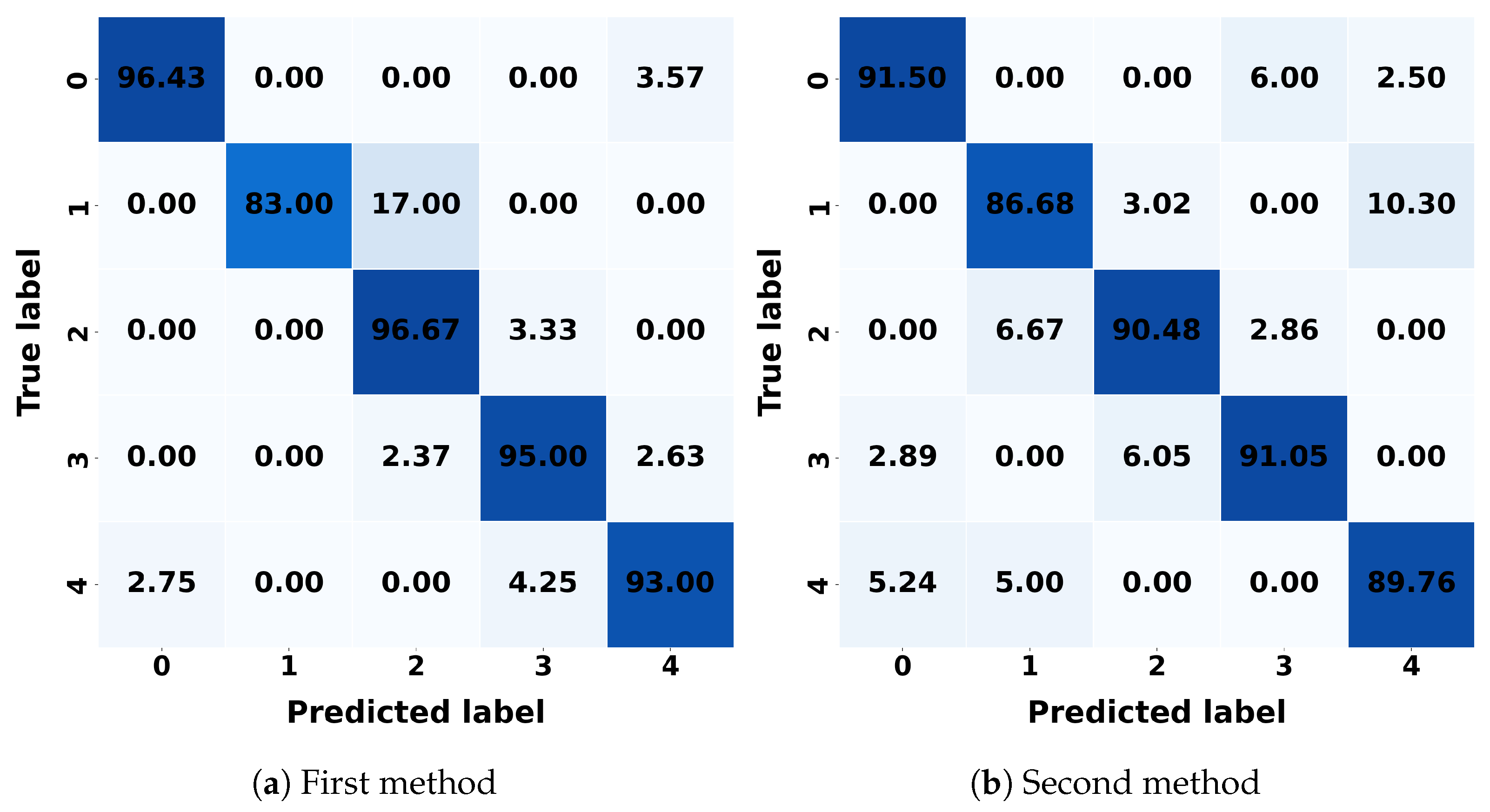
For k-NNs, the first method correctly classifies 97.75% of class 1, with a misclassification rate of 2.25% as class 2. In the second method, k-NNs achieves a correct classification rate of 91.25% for class 2, with a misclassification rate of 6.25% as class 3. LR correctly classifies 99.29% of class 0 in the first method, with a misclassification rate of 0.71% as class 4. In the second method, it also correctly classifies 92.89% of class 3, with a misclassification rate of 4.21% as class 2. DT correctly classifies 95.25% of class 1 in the first method, with a misclassification rate of 4.75% as class 2. In the second method, DT achieves a correct classification rate of 92.11 as class 3%, with a misclassification rate of 5.26% as class 2. RF achieves a correct classification rate of 98.25% for class 1 in the first method, with a misclassification rate of 1.75% as class 2. In the second method, it incorrectly classifies 6.25% as class 3, with a correct classification rate of 92%. SVM correctly classifies 97.62% as class 2 in the first method, with a misclassification rate of 2.38% as class 3. In the second method, SVM achieves a correct classification rate of 92.89% as class 3, with a misclassification rate of 4.21% as class 2. NB correctly classifies 96.58% as class 3 in the first method, with a misclassification rate of 1.84% as class 2. In the second method, it achieves a correct classification rate of 94.21% as class 3, with a misclassification rate of 3.42%. LDA correctly classifies 99.21% as class 3 in the first method, with a misclassification rate of 0.79% as class 4. In the second method, it achieves a correct classification rate of 95.53% as class 3, with a misclassification rate of 3.16% as class 0. QDA correctly classifies 96.67% as class 2 in the first method, with a misclassification rate of 3.33% as class 3. In the second method, it achieves a correct classification rate of 91.50% as class 0, with a misclassification rate of 2.50% as class 4.
6. Discussion and Comparative Analysis
The comparative analysis highlights the consistent superiority of RF across all scaling techniques and training methods. RF achieved the highest accuracy (up to 94.95%), RMSE, and strong
scores (up to 90.46%), demonstrating its robustness and adaptability. In comparison, Xia et al. [
16] attained a slightly higher accuracy of 95.09% using a CNN-BiLSTM model. This was enabled by combining local feature extraction from CNN with temporal feature modeling from BiLSTM, utilizing inertial measurement units and plantar pressure sensors for data acquisition. However, the complexity and increased hardware requirements of this approach may limit its practicality in certain scenarios. SVM also showed strong performance in this study, particularly under SS and PCA, with high accuracy and low RMSE. Similarly, LR and k-NNs performed well but did not match the predictive accuracy of RF and SVM. In comparison, the study by Ma et al. [
15] demonstrated real-time robustness and generalization capabilities using joint angular sensors in the hip and knee joints, achieving an accuracy of 88.71%. However, its accuracy falls short compared to RF and advanced models like CNN-BiLSTM. In contrast, NB, LDA, and QDA underperformed in this study, with higher error rates and lower
scores.
These findings emphasize the importance of selecting appropriate preprocessing techniques, training strategies, and ML models. While RF is the most adaptable and robust in the current study, integrating advanced architectures like CNN-BiLSTM could enhance performance if hardware complexity is appropriately managed. Furthermore, the practical implications of these results can be extended to clinical gait analysis, where RF’s strong predictive capabilities could support real-time gait monitoring in rehabilitation settings. The implementation of RF in wearable devices could aid in the early detection of abnormal gait patterns, enabling timely intervention for patients with mobility impairments. Additionally, hybrid models combining traditional ML and DL approaches may offer a balance between computational efficiency and classification accuracy, making them viable solutions for real-world deployment.
Future research could explore domain adaptation techniques to improve model generalization across diverse populations, as well as multi-sensor data fusion strategies that integrate data from inertial sensors, force plates, and depth cameras. By addressing these challenges, gait classification models can become more robust and applicable to broader clinical and biomechanical applications.
7. Conclusions
This study provides a comprehensive analysis of gait phase classification using ML techniques, emphasizing the importance of scaling methods and training strategies. Among the evaluated models, RF consistently outperformed others across all scaling techniques, achieving high accuracy, low error rates, and robust scores. SVM also demonstrated strong performance, particularly under Standard Scaling and PCA, highlighting their potential for complex classification tasks. Key insights from this study include the impact of scaling techniques like Min–Max Scaling, Standard Scaling, and PCA on model performance, and the importance of selecting appropriate training strategies to ensure robust and generalizable results. These findings underscore the critical role of preprocessing and algorithm selection in optimizing classification accuracy for clinical and real-world applications.
Beyond theoretical contributions, this study has significant practical advantages, particularly in the fields of biomechanics, rehabilitation, and assistive technologies. The proposed machine learning models can be integrated into real-time gait monitoring systems, enabling continuous tracking of gait patterns and early detection of abnormalities. Additionally, these models offer valuable support for clinicians in assessing rehabilitation progress for patients with neurological disorders such as Parkinson’s disease and stroke. The insights gained from this research also contribute to the development of intelligent prosthetics and robotic exoskeletons, enhancing mobility assistance for individuals with motor impairments. Furthermore, accurate gait phase classification can play a key role in fall prevention systems by assessing gait stability and issuing alerts for individuals at high risk of falls, particularly among elderly or mobility-impaired populations. Finally, in sports science, these models can optimize athletic performance and minimize injury risks through biomechanical gait analysis, demonstrating the broad applicability of this research in both medical and non-medical fields.
Future research could focus on integrating DL architectures, such as CNNs and recurrent neural networks (RNNs), to capture temporal and spatial dependencies in gait data. Additionally, exploring hybrid models and multi-modal datasets could further enhance the accuracy and reliability of gait phase classification. Finally, the implementation of these models in real-time systems for rehabilitation, sports analytics, and patient monitoring represents a promising avenue for translating these insights into practical applications.


