Efficient Scheduling for GPU-Based Neural Network Training via Hybrid Reinforcement Learning and Metaheuristic Optimization

Abstract

On GPU-based clusters, the training workloads of machine learning (ML) models, particularly neural networks (NNs), are often structured as Directed Acyclic Graphs (DAGs) and typically deployed for parallel execution across heterogeneous GPU resources. Efficient scheduling of these workloads is crucial for optimizing performance metrics such as execution time, under various constraints including GPU heterogeneity, network capacity, and data dependencies. DAG-structured ML workload scheduling could be modeled as a Nonlinear Integer Program (NIP) problem, and is shown to be NP-complete. By leveraging a positive correlation between Scheduling Plan Distance (SPD) and Finish Time Gap (FTG) identified through an empirical study, we propose to develop a Running Time Gap Strategy for scheduling based on Whale Optimization Algorithm (WOA) and Reinforcement Learning, referred to as WORL-RTGS. The proposed method integrates the global search capabilities of WOA with the adaptive decision-making of Double Deep Q-Networks (DDQN). Particularly, we derive a novel function to generate effective scheduling plans using DDQN, enhancing adaptability to complex DAG structures. Comprehensive evaluations on practical ML workload traces collected from Alibaba on simulated GPU-enabled platforms demonstrate that WORL-RTGS significantly improves WOA’s stability for DAG-structured ML workload scheduling and reduces completion time by up to 66.56% compared with five state-of-the-art scheduling algorithms.

1. Introduction

On GPU-based clusters for machine learning (ML) training, a significant portion of resources is dedicated to long-running workloads, often modeled as Directed Acyclic Graphs (DAGs) [1,2]. These workloads, prevalent in large-scale ML applications such as Deep Neural Network (DNN) training, consist of tasks with complex dependencies, managed by resource orchestration frameworks such as Kubernetes [3], Apache Hadoop YARN [4], or Apache Mesos [5]. The nodes in a DAG represent tasks, while the edges denote data dependencies, making efficient scheduling critical for optimizing performance metrics such as execution time. Despite extensive efforts, scheduling DAG-structured ML tasks in GPU environments remains challenging due to the trade-offs between data transfer overheads in distributed schedules and task waiting times in centralized ones.

Deploying ML workloads on a GPU cluster faces unique scheduling difficulties, particularly when relying on heuristic rules or ML-driven decision-making. Reinforcement Learning (RL) approaches, including Deep Q-Networks (DDQN) [6], attempt to discover effective policies by capturing task dependencies and the dynamics of resource availability. However, these methods face drawbacks such as expensive training costs, large data requirements, and poor adaptability when applied to heterogeneous GPU platforms or varied DAG topologies. Whereas heuristic-based strategies such as Genetic Algorithms (GAs) and Whale Optimization Algorithm (WOA) [7] offer computationally lightweight solutions, they frequently stagnate in non-optimal states or perform poorly in discrete and high-dimensional DAG scheduling, where conventional distance measures fail to represent plan similarity effectively.

In our previous research [8], we modeled the scheduling of DAG-structured workloads as a Nonlinear Programming (NLP) problem, termed as Long-Running Workload Task Scheduling (LRW-TS), and proved its NP-completeness. We identified a positive correlation between Scheduling Plan Distance (SPD) and Finish Time Gap (FTG), and by leveraging this finding, we designed RTGS, a hybrid approach combining WOA with a Greedy strategy. Our work in this paper extends that foundation to GPU-based ML training, replacing the Greedy algorithm with a Double Deep Q-Network (DDQN) to establish a novel scheduling solution, referred to as WORL-RTGS. By exploiting the SPD-FTG correlation, we redefine Scheduling Plan Distances, enabling WOA to effectively handle complex DAG dependencies in heterogeneous GPU environments. The WORL-RTGS integration mitigates the limitations of standalone RL (e.g., slow convergence) and traditional heuristics (e.g., local optima traps), achieving superior makespan and resource utilization. Key challenges addressed include

• Measuring Scheduling Plan Distances: We use FTG as a proxy for distance, converting it to SPD via the identified correlation.
• Generating controlled scheduling plans: DDQN dynamically generates plans with precise distances, improving over the rigidity of a Greedy approach.

Empirical evaluations using real-world ML workload traces from Alibaba in simulated GPU environments demonstrate that WORL-RTGS reduces completion time by up to 66.56% compared with state-of-the-art baselines. The proposed approach excels on heterogeneous GPU clusters, adapting to diverse DAG structures and resource constraints while maintaining stability. Our key contributions are summarized as follows:

• Formulate the Neural Network with Hybrid Parallel (N2HP) scheduling problem and prove its NP-completeness.
• Leverage the SPD-FTG correlation to redefine Scheduling Plan Distances for GPU-based ML tasks.
• Design WORL-RTGS, a hybrid scheduler combining WOA’s global search with DDQN’s adaptive decision-making, outperforming traditional heuristics and RL methods.
• Introduce a generalizable framework for DAG-structured ML task scheduling, opening new research directions.

The rest of the paper is organized as follows: Section 2 surveys related work, highlighting limitations of swarm intelligence for task scheduling. Section 3 formulates the N2HP problem and analyzes its complexity. Section 4 details the design of the WORL-RTGS algorithm, leveraging the SPD-FTG correlation. Section 5 evaluates performance against baselines. Section 6 concludes our work and sketches future efforts.

2. Related Work

Recent advancements in intelligent task scheduling for cloud computing and deep learning (DL) environments address resource optimization and quality of service (QoS). In three-tier cloud marketplaces, SaaS providers aim to minimize VM leasing costs while ensuring QoS for dynamic workloads. A two-layer DQN-based framework integrates QoS-aware task assignment with elastic VM auto-scaling, improving resource utilization and reducing costs [9]. For DAG-structured workloads in heterogeneous real-time systems, novel node-priority assignment strategies leveraging global DAG structures achieve up to 14.35% makespan improvement over baselines [10].

In GPU-based distributed DL training, Chronus [11] supports deadline-constrained and best-effort jobs by exploiting DL workload characteristics like predictability and preemptibility, enhancing SLO satisfaction and completion time. Datacenter-level analysis, such as SenseTime’s trace study, informs quasi-shortest-service-first policies and energy-saving managers, boosting cluster utilization and reducing latency [12]. For hybrid clouds, DRL-based VM selection optimizes execution cost and QoS under fluctuating workloads [13].

For safety-critical tasks on many-core platforms, DAG-Order [14] uses non-preemptive scheduling on SLT NoC architectures, ensuring safe response times and outperforming state-of-the-art methods. Multi-core systems face multi-DAG interference, addressed by improved scheduling schemes that model core allocation constraints, enhancing schedulability [15]. In DNN training, DAPPLE [16] combines data and pipeline parallelism with intelligent scheduling, improving throughput and memory efficiency over GPipe and PipeDream.

Reinforcement Learning (RL) schedulers show promise in dynamic environments. The A2C Scheduler [17] reduces gradient estimation variance, outperforming policy gradient methods. DRL-based edge computing solutions using DQNs adaptively schedule workloads, improving service time and task success rates [18]. For GPU datacenters, DL2 [19] integrates supervised and RL to reduce job completion times, while a survey [20] categorizes DL workload characteristics and future scheduling directions.

Large-scale Transformer models benefit from TeraPipe’s token-level pipeline parallelism, reducing training time via dynamic programming [21]. PipePar [22] enhances load balancing on heterogeneous GPU clusters by considering performance diversity and bandwidth. DRL-based schedulers handle dynamic resource demands, with workload clustering to improve scalability [23] and Spark cluster scheduling to optimize cost and performance [24].

Multi-objective optimization in cloud scheduling, such as Pareto-efficient schedulers, minimizes makespan and communication costs [25]. MORL-WS [26] uses multi-objective RL for workflow scheduling, improving makespan and energy efficiency. Systems like Liquid [27] and Horus [28] enhance GPU resource sharing by addressing interference, improving job completion times and utilization.

In High-Performance Computing (HPC), DRAS [29] employs hierarchical DRL scheduling, outperforming heuristics by up to 50% on real workloads. Hierarchical partitioning for GPU co-scheduling achieves 1.87× throughput improvement [30]. Multi-agent RL frameworks [31] and mDRL [32] reduce job completion time and power consumption on large-scale GPU clusters. DeepShare [33] mitigates network contention, cutting job completion times by up to 20.7%.

These studies highlight the trend toward hybrid, learning-based, and system-aware scheduling, leveraging RL and workload characteristics to optimize performance across diverse computing platforms. Our work proposes a novel scheduling approach, WORL-RTGS, to deal with complex task dependencies in heterogeneous cloud environments by integrating the WOA algorithm with the DDQN algorithm. A key discovery is the positive correlation between two critical variables, enabling variable transformation to adapt WOA for efficiently handling intricate task scheduling with strict dependencies. This hybrid WORL-RTGS method overcomes limitations of traditional heuristic algorithms, such as local optima traps, and standalone RL approaches, which often suffer from high computational overhead and slow convergence. The synergy of WOA’s global search capability and DDQN’s adaptive decision-making ensures robust performance, achieving superior makespan and resource utilization compared with existing methods.

3. Problem Formulation

3.1. Cost Model for Neural Network Training with Hybrid Parallelism

The distribution of neural network training across multiple GPUs and servers depends on the adopted parallelization strategy. In distributed parallel processing systems, three main types of parallelism are commonly employed as follows: data parallelism, model parallelism, pipeline parallelism, and hybrid parallelism, as briefly described below.

• Data Parallelism: The entire neural network model is replicated on each GPU/server. Different subsets of data are distributed to each GPU. After each forward and backward pass, gradients from all GPUs are averaged (or summed) across the devices (e.g., via AllReduce [34]) before updating the model. This parallelism is considered when the model fits in a single GPU’s memory, but training data is large.
• Model Parallelism: The model is split spatially by layers or by tensor dimensions across multiple GPUs. The splitting method is usually structure-agnostic or based on tensor shapes or layer sizes, not the functional purpose of model components. Forward/backward pass is conducted sequentially across GPUs. The purpose of this parallelism is to train a large model that does not fit in a single GPU.
• Pipeline Parallelism: This parallelism divides the model into stages, and each GPU handles a stage. Splitting into stages is conducted intentionally, with functional awareness (e.g., grouping layers that form logical blocks or stages of computation). To improve GPU utilization, the input mini-batch of training samples is divided into smaller micro-batches, which are fed into the pipeline in a staggered fashion, allowing different micro-batches to flow through different GPUs concurrently. Pipeline parallelism is useful when training large models that do not fit in a single GPU but also require efficient hardware usage.
• Hybrid Parallelism: A hybrid approach combines two or more parallelization strategies: data parallelism, model parallelism, and pipeline parallelism, to efficiently train large-scale models on multi-GPU and multi-server systems. It is used when no single type of parallelism is sufficient alone, especially for very large neural networks such as GPT-3 [35] or GPT-4 [36] that far exceed the memory and compute capacity of a single GPU.

We define the cost model to support the scheduling of neural network (NN) training workloads on multi-GPU, multi-server platforms using hybrid parallelism, which combines data parallelism, model parallelism, and pipeline parallelism. A computational unit represents either a complete layer, a partitioned sublayer due to model parallelism, or a group of layers or sublayers forming a pipeline stage. Note that a computational unit may contain neurons from multiple layers. We represent each layer within a computational unit as a single node, as shown in Figure 1. The nodes belonging to the same computational unit should be scheduled onto the same GPU for processing. A neural network training job is modeled as a Directed Acyclic Graph (DAG) $G_{NN}=\left\{L,E_L,W,M,D\right\}$, where $L=\left\{l_1,l_2,\dots ,l_n\right\}$ is the set of n nodes, $E_L=\left\{(l_i,l_j)\mid l_i,l_j\in L\right\}$ defines the forward/backward computational dependencies between nodes, $W=\left\{w_1,w_2,\dots ,w_n\right\}$ is the computational workload, e.g., in unit of FLoating point OPerations (FLOPs) [37], for the n nodes, $M=\left\{m_1,m_2,\dots ,m_n\right\}$ represents the GPU memory requirement of each node, and $D=\left\{d_{ij}\mid l_i,l_j\in L\right\}$ is the size of the data such as activations or gradients transferred between dependent nodes. Let $CU=\left\{c{u}_1,c{u}_2,\dots ,c{u}_p\right\}$ denote the set of computational units. Each unit $c{u}_q\subseteq L$ consists of a subset of nodes that must be co-located on the same GPU. The exact granularity of each $l_i\in L$ and $c{u}_q\subseteq L$ depends on the adopted parallelization strategy. Figure 1 illustrates an example of a neural network training job that incorporates data parallelism, model parallelism, and pipeline parallelism, respectively.

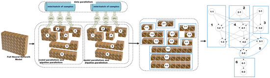
Figure 1. An example of a neural network training job with data parallelism, model parallelism, and pipeline parallelism.

We model the training platform as a GPU cluster $G_{GPU}=\left\{G,S,E_G,C,B\right\}$, where $G=\left\{g_1,g_2,\dots ,g_m\right\}$ denotes the set of m available GPUs across all servers on the training platform, $S=\left\{s_1,s_2,\dots ,s_k\right\}$ denotes the set of k servers, $E_G=\left\{(g_i,g_j)\mid g_i,g_j\in G\right\}$ denotes the set of interconnections between GPUs, $C=\left\{c_1,c_2,\dots ,c_m\right\}$ denotes the set of computational capabilities of each GPU, e.g., in unit of Tera FLoating point OPerations Per Second (TFLOPS) [38], and $B=\left\{b_{ij}\mid (g_i,g_j)\in E_G\right\}$ denotes the bandwidth between two connected GPUs $g_i$ and $g_j$. We define a function $\mathrm{host}\left(g_i\right)\in S$ that maps each GPU $g_i\in G$ to a server and a mapping function $\mathrm{map}\left(l_i\right)\in G$ that assigns each node $l_i$ to a GPU $g_k$ for execution. For any pair of nodes $l_i,l_j\in L$ that belong to the same computational unit, we enforce $\mathrm{map}\left(l_i\right)=\mathrm{map}\left(l_j\right)$. For each pair $(g_i,g_j)\in E_G$, if $\mathrm{host}\left(g_i\right)=\mathrm{host}\left(g_j\right)$, the interconnection is classified as intra-server; otherwise, if $\mathrm{host}\left(g_i\right)\ne \mathrm{host}\left(g_j\right)$, it is classified as inter-server. The value of $b_{ij}$ depends on the type of interconnect. If $g_i$ and $g_j$ are on the same server and connected via NVLink, then $b_{ij}$ reflects the NVLink bandwidth (e.g., 50–600 GB/s depending on hardware generation). If $g_i$ and $g_j$ reside on different servers, then $b_{ij}$ represents the inter-server communication bandwidth, typically provided by Remote Direct Memory Access (RDMA) technologies or high-speed Ethernet. Figure 2 illustrates a GPU cluster consisting of two servers, along with an example of computational unit allocation.

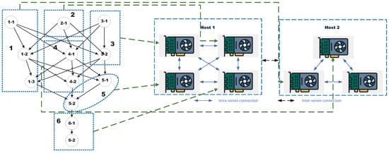
Figure 2. A GPU cluster with two servers and an example of computational unit allocation.

The total training time for a mini-batch depends on the following factors:

• Node Execution Time: Each node $l_i$ has an execution time dependent on its computational workload $w_i$ and the GPU capability $c_k$ of the assigned GPU $g_k$.
• Data Transfer Time: For two dependent nodes $l_i\to l_j$, if they are placed on different GPUs $g_k$ and $g_l$, the data transfer time is governed by $d_{ij}$ and bandwidth $b_{kl}$ between $g_k$ and $g_l$.
• Stall Time: In both pipeline and model parallelism, adjacent stages or model partitions may experience stall time due to imbalances in execution time across stages or model parts.
• Synchronization Time: In data parallelism, all GPUs must synchronize gradients at the end of each backward pass, hence introducing communication overheads.

The optimization goal is to minimize hybrid parallel training cost for one iteration (mini-batch) by scheduling computational units to GPUs in a way that balances workloads, minimizes inter-GPU communication, and avoids stall time caused by pipeline and model parallelism.

3.2. Formulation of the Scheduling Problem for NN Training

We investigate how a DAG-structured neural network training task executes, formulate the scheduling problem as a nonlinear integer programming model, and prove its NP-completeness.

A node $l\in L$ is considered as an entry node if it has no predecessors, i.e., there is no $l_p\in L$ with $(l_p,l)\in E_L$. For such a node, the earliest start time $\mathit{EST}\left(l\right)$ is 0; otherwise, $\mathit{EST}\left(l\right)$ is determined by the maximum arriving time ($\mathit{AT}$) among all data produced by its immediate predecessors:

$$\mathit{EST}\left(l\right)=\left\{\begin{array}{c}0,\mathrm{if} l=entry node;\hfill \\ {\max }_{l\prime \in precede\left(l\right)}\mathit{AT}(l\prime ,l),\mathrm{else}.\hfill \end{array}\right.$$

(1)

Equation (1) defines the earliest start time $\mathit{EST}\left(l\right)$ of node l. If l is an entry node with no predecessors, then $\mathit{EST}\left(l\right)=0$, meaning that it can start execution immediately without waiting for any input; otherwise, $\mathit{EST}\left(l\right)$ depends on the latest arrival time $\mathit{AT}(l^{\prime },l)$ of data produced by all its immediate predecessor nodes $l^{\prime }$, using the maximum to ensure that l can begin to execute only after all dependency data are ready, thereby enforcing the topological order constraints in the DAG.

The data arrival time from a predecessor node $l_i$ is given by the actual finish time $\mathit{AFT}\left(l_i\right)$ plus the transmission delay $\mathit{Trans}(l_i,l_j)$ required to transfer results from the GPU executing $l_i$ to the GPU assigned to its successor $l_j$:

$$\mathit{AT}\left(l_i,l_j\right)=\mathit{AFT}\left(l_i\right)+\mathit{Trans}\left(l_i,l_j\right).$$

(2)

Equation (2) computes the data arrival time $\mathit{AT}(l_i,l_j)$ from predecessor node $l_i$ to successor node $l_j$, which equals the actual finish time $\mathit{AFT}\left(l_i\right)$ of $l_i$ plus the cross-GPU data transmission delay $\mathit{Trans}(l_i,l_j)$. This equation captures the direct impact of communication overhead on task start time, particularly in model parallelism or pipeline parallelism scenarios, where significant delay may occur if $l_i$ and $l_j$ are on different GPUs, potentially postponing the execution of $l_j$.

The data transmission time from the GPU running node $l_{\mathrm{i}}$ to the GPU running node $l_{\mathrm{j}}$ is calculated as

$$Trans\left(l_{\mathrm{i}},l_{\mathrm{j}}\right)={\displaystyle \frac{d\left(l_{\mathrm{i}},l_{\mathrm{j}}\right)}{b\left(\mathrm{map}\left(l_{\mathrm{i}}\right),\mathrm{map}\left(l_{\mathrm{j}}\right)\right)}},$$

(3)

where $d(l_i,l_j)$ represents the volume of data transferred from predecessor $l_i$ to successor $l_j$, $b(\mathrm{map}\left(l_i\right),\mathrm{map}\left(l_j\right))$ denotes the bandwidth between the GPUs executing $l_i$ and $l_j$, and $\mathrm{map}\left(l_i\right)$ specifies the GPU assigned to node $l_i$. Equation (3) provides the precise calculation of data transmission time $\mathit{Trans}(l_i,l_j)$: the data volume $d(l_i,l_j)$, such as activations or gradients, divided by the actual bandwidth $b(\mathrm{map}\left(l_i\right),\mathrm{map}\left(l_j\right))$ between the GPUs executing $l_i$ and $l_j$. This formula highlights the strong correlation between communication cost and scheduling mapping: if two nodes are mapped to the same GPU, $b\to \infty$ (theoretically no transmission delay); if across servers, b is small, leading to large delays, and hence incentivizing the scheduler to prioritize placing strongly dependent nodes on high-bandwidth links.

If GPU g has sufficient Available Resources ($\mathit{AvailR}$) to run node l at its earliest start time $\mathit{EST}\left(l\right)$, then the actual start time $\mathit{AST}\left(l\right)$ is $\mathit{EST}\left(l\right)$; otherwise, the execution of l is delayed until GPU g provides Sufficient Resources ($\mathit{SufR}$). The value of $\mathit{AST}\left(l\right)$ is calculated as

$$\mathit{AST}\left(l\right)=\left\{\begin{array}{c}\mathit{EST}\left(l\right),\mathrm{if}\mathit{AvailR}\left(g,\mathit{EST}\left(l\right)\right)>m_{\mathrm{l}}\hfill \\ \mathit{SufR}\left(g,l\right),\mathrm{else}\hfill \end{array}\right.$$

(4)

where $\mathit{AvailR}\left(g,\mathit{EST}\left(l\right)\right)$ represents the memory available on GPU g at time $\mathit{EST}\left(l\right)$. Equation (4) determines the actual start time $\mathit{AST}\left(l\right)$ of node l, considering the dynamic availability of GPU memory resources. If, at the earliest possible start time $\mathit{EST}\left(l\right)$, the available memory $\mathit{AvailR}(g,\mathit{EST}(l\left)\right)$ on the target GPU g exceeds the memory required by node l ($m_l$), then no delay is needed and execution starts immediately; otherwise, it must be postponed until the time $\mathit{SufR}(g,l)$ when the GPU releases sufficient memory. This mechanism prevents memory over-allocation and simulates execution blocking due to insufficient GPU memory in real training scenarios.

We determine $\mathit{AvailR}$ for GPU g at a given time point as

$$\mathit{AvailR}\left(g,\mathit{time}\right)=\mathit{AllMem}\left(g\right)-\mathit{UsedM}\left(g,\mathit{time}\right),$$

(5)

where $\mathit{UsedM}\left(g,\mathit{time}\right)$ denotes the occupied memory on GPU g at $\mathit{time}$. Equation (5) straightforwardly defines the available memory on GPU g at any time $\mathit{time}$: total memory capacity $\mathit{AllMem}\left(g\right)$ minus the currently occupied memory $\mathit{UsedM}(g,\mathit{time})$. This expression serves as the foundation for subsequent memory scheduling decisions, ensuring that tasks exceeding remaining memory are not assigned to the GPU, avoiding runtime Out-of-Memory (OOM) errors.

The value of $\mathit{UsedM}\left(g,\mathit{time}\right)$ is calculated as

$$\mathit{UsedM}\left(g,\mathit{time}\right)=\sum _{l\in L}{m}_{\mathrm{l}}·x\left(l,g\right)·\max \left\{0,{\displaystyle \frac{\mathit{AFT}\left(l\right)-\mathit{time}}{\left|\mathit{AFT}\left(l\right)-\mathit{time}\right|}}\right\},$$

(6)

where $m_{\mathrm{l}}$ is the memory required for node l, and $x(l,g)$ is 1 if node l is assigned to GPU g, and 0, otherwise. Meanwhile, $\mathit{SufR}(g,l)$ indicates the earliest time when GPU g has sufficient resources to execute node l. Equation (6) accurately accounts for the used memory on GPU g at time $\mathit{time}$: for all nodes l assigned to this GPU (marked by $x(l,g)=1$), if their actual finish time $\mathit{AFT}\left(l\right)>\mathit{time}$ (i.e., still executing or just completed but memory not yet released), their memory requirement $m_l$ is included in the sum; otherwise, it contributes 0. This piecewise function simulates the lifecycle of memory occupancy via sign judgment, counting memory only during the active period of tasks, reflecting the dynamic allocation and release behavior of intermediate results such as activations and gradients in training.

The value of $\mathit{SufR}(g,l)$ is computed as

$$\mathit{SufR}\left(g,l\right)=\min \left\{\mathit{AFT}\left(l^{\prime }\right)\left|\begin{array}{c}{l}^{\prime }\in L,\hfill \\ x\left(l^{\prime },g\right)=1,\hfill \\ \mathit{AvailR}\left(g,\mathit{AFT}\left(l^{\prime }\right)\right)⩾m_{\mathrm{l}}\hfill \end{array}\right.\right\}.$$

(7)

Equation (7) provides the earliest executable time $\mathit{SufR}(g,l)$ that node l must wait for when GPU g has insufficient memory: among all tasks $l^{\prime }$ already assigned to g, find the completion time $\mathit{AFT}\left(l^{\prime }\right)$ such that after $l^{\prime }$ finishes, the available memory on the GPU first meets the demand $m_l$ of l, and take the minimum of such $\mathit{AFT}\left(l^{\prime }\right)$. This equation essentially identifies the critical points of memory release, ensuring that l does not start earlier than resource readiness, embodying the serialization scheduling constraints in resource-constrained environments.

Additional constraints on DAG workload execution include the following:

$$\begin{array}{cccc}\hfill x\left(l,g\right)& =& 0\mathrm{or}1,\hfill & l\in L,g\in G,\hfill \end{array}$$

(8)

$$\begin{array}{cccc}\hfill z\left(g,s\right)& =& 0\mathrm{or}1,\hfill & g\in G,s\in S,\hfill \end{array}$$

(9)

$$\begin{array}{cccc}\hfill \sum _{g\in G}x\left(l,g\right)& =& 1,\hfill & l\in L,\hfill \end{array}$$

(10)

$$\begin{array}{cccc}\hfill \sum _{s\in S}z\left(g,s\right)& =& 1,\hfill & g\in G,\hfill \end{array}$$

(11)

$$\begin{array}{cccc}\hfill \mathit{map}\left(l\right)& =\sum _{g\in G}x\left(l,g\right)·g,\hfill & \hfill & l\in L,\hfill \end{array}$$

(12)

$$\begin{array}{cccc}\hfill \mathit{host}\left(g\right)& =\sum _{s\in S}z\left(g,s\right)·s,\hfill & \hfill & g\in G,\hfill \end{array}$$

(13)

$$\begin{array}{cccc}\hfill ext\left(l\right)& ={\displaystyle \frac{w_l}{c\left(\mathrm{map}\left(l\right)\right)}},\hfill & \hfill & l\in L,\hfill \end{array}$$

(14)

$$\begin{array}{cccc}\hfill \mathit{AFT}\left(l\right)& =\mathit{AST}\left(l\right)+rt\left(l\right),\hfill & \hfill & l\in L,\hfill \end{array}$$

(15)

$$\begin{array}{cccc}\hfill \mathrm{map}\left(l_i\right)& =\mathrm{map}\left(l_j\right),\hfill & \hfill & l_i,l_j\in c{u}_q,\forall c{u}_q\in CU.\hfill \end{array}$$

(16)

Constraints (8)–(16) form the core integer linear constraint system of the scheduling problem. Among them, Equations (8) and (9) declare $x(l,g)$ and $z(g,s)$ as binary assignment variables; Equation (10) ensures that each node l is assigned to exactly one GPU; Equation (11) ensures that each GPU belongs to exactly one server; Equations (12) and (13) define the mapping functions $\mathit{map}\left(l\right)$ and $\mathit{host}\left(g\right)$ via weighted sums, facilitating reference to actual devices in the objective; Equation (14) computes the execution time $ext\left(l\right)$ of node l on its assigned GPU, i.e., workload $w_l$ divided by the compute capability $c\left(\mathit{map}\right(l\left)\right)$ of that GPU, reflecting performance differences in heterogeneous hardware; Equation (15) obtains the finish time from actual start time plus execution time; and Equation (16) forces all nodes within the same computational unit $c{u}_q$ to be mapped to the same GPU, preserving locality in model parallelism or pipeline stages and preventing communication explosion due to unnecessary cross-device partitioning.

The objective of a scheduler is to minimize the final finish time ($\mathit{FFT}$) of a DAG-structured neural network training job:

$$\mathit{FFT}=\max \left\{\mathit{AFT}\left(l\right)\left|l\in L\right.\right\}.$$

(17)

The objective function in Equation (17) defines the ultimate metric of scheduling optimization as the maximum of the actual finish times $\mathit{AFT}\left(l\right)$ of all nodes in the DAG, i.e., the total time $\mathit{FFT}$ to train one mini-batch. Minimizing $\mathit{FFT}$ is equivalent to compressing the critical path length while balancing various bottlenecks from computation, communication, and memory contention, making it the core optimization goal of the hybrid parallel training scheduling problem.

We formally define the Neural Network with Hybrid Parallel (N2HP) scheduling problem as follows:

Definition 1 

(N2HP). Let $G_{NN}=\{L,E_L,W,M,D\}$ represent a DAG-structured training job and $G_{GPU}=\{G,S,E_G,C,B\}$ denote a parallel computing platform. The scheduling objective is to determine a schedule that minimizes $\mathit{FFT}$ subject to the precedence constraints and resource limitations established in Equations (1)–(16).

3.3. Analysis of Computational Complexity

In this section, we show that N2HP is NP-complete. We begin by presenting the set partition problem, one of Karp’s 21 NP-complete problems [39], and then show a polynomial-time reduction from it to N2HP.

Set Partition Problem: The problem is to split a set Q into two disjoint subsets with equal sums. Let $A\subseteq Q$ have sum $Q_1$. The problem asks if the remaining elements $(Q-A)$ form a subset with sum $Q_2$ such that $Q_1=Q_2$.

Theorem 1. 

N2HP belongs to the class of NP-complete problems.

Proof. 

For the decision version of N2HP, we consider a DAG-structured job defined by $G_{NN}=\{L,E_L,W,M,D\}$, a GPU-based parallel computing system $G_{GPU}=\{G,S,E_G,C,B\}$, and a performance limit l. The question is if a scheduling approach exists that achieves $\mathit{FFT}\le l$.

To demonstrate that N2HP belongs to NP, we begin by confirming that $\mathit{FFT}$ can be computed in polynomial time under any given schedule. Starting with a DAG, we apply topological sorting to arrange its vertices in linear time, as described in Cormen et al. [40]. Using this order, we compute the longest paths from a chosen starting vertex by processing each vertex and determining the maximum path length through its incoming edges, also in linear time [41]. The $\mathit{FFT}$ is then derived by identifying the longest path among all entry nodes in polynomial time. Thus, for any scheduling plan, we can efficiently calculate $\mathit{FFT}$, compare it to the threshold l, and verify the solution, thereby confirming that N2HP is in NP.

To establish the NP-hardness of N2HP, we consider a simplified instance of N2HP with a specific network structure. The simplified job consists of n task nodes, including $n-1$ entry nodes and a single exit node. The computing platform comprises two identical GPUs on a server. The execution time of the exit node, as well as all data transfer costs from the entry nodes to the exit node, are considered negligible. Under these conditions, the DAG reduces to a star topology, while the platform becomes two homogeneous GPUs without bandwidth limitations. This abstraction eliminates the effects of communication delays and dependency overheads, isolating the node placement problem for analysis. Although not encompassing complete intricacy of practical N2HP situations, this treatment demonstrates that computational difficulty endures even in this severely simplified scenario. The goal of minimizing the job’s completion time can be reduced to the problem of splitting the entry nodes’ execution times into two collections with matching sums. This specific case of N2HP can be directly transformed to the classic set partition problem [39]: the set Q denotes the execution times of entry nodes, subset A represents those entry nodes allocated to one GPU, and $(Q-A)$ represents those entry nodes assigned to the other. This reduction establishes that N2HP is computationally not easier than the set partition problem. Given that the reduction executes in polynomial time and N2HP ∈ NP, we prove that N2HP is NP-complete.    □

4. Design of the Proposed Algorithm

Given the NP-completeness of N2HP established in Section 3.3, no polynomial-time algorithm exists that guarantees optimal solutions unless $P=NP$. This section presents the design of the Whale Optimization and Reinforcement Learning-based Running Time Gap Strategy (WORL-RTGS). First, we introduce a variable to quantify the gap between scheduling strategies and demonstrate its positive correlation with the running time difference between two scheduling schemes. Then, inspired by the hunting behavior of humpback whales, we design a time-difference Whale Optimization method to control the positioning of new whales during the generation of candidate scheduling schemes. The time-difference Whale Optimization method consists of three components, each representing a mechanism by which the scheduling plan iteratively approaches the optimal solution. Finally, based on the inference results of the time-difference Whale Optimization method, we design a Double Deep Q-Network (DDQN)-based method to locate the position matrix of new whales.

4.1. Introduction to the WOA

The WOA is a nature-inspired metaheuristic modeled on the social hunting behavior of humpback whales, especially their Bubble-Net Feeding Strategy. The WOA iteratively transitions between exploration (global search) and exploitation (local search). Using different mathematical formulations for these phases, WOA maintains a balance between wide-ranging search and precise local optimization. The algorithm simulates key behaviors such as the Spiral Bubble-Net Attack and Prey Encircling through subsequent procedures:

• Encircling Prey:

Whales identify the position of their prey and proceed to envelop it. This behavior is represented mathematically as

$$\overrightarrow{Di}s=|\overrightarrow{Co}e·\overrightarrow{X^{\ast }}\left(t\right)-\overrightarrow{X}\left(t\right)|,$$

(18)

$$\overrightarrow{X}(t+1)=\overrightarrow{X^{\ast }}\left(t\right)-\overrightarrow{Ac}·\overrightarrow{Di}s,$$

(19)

where $\overrightarrow{X^{\ast }}(t)$ represents the current best solution’s position, $\overrightarrow{X}(t)$ is the position vector of a whale, and $\overrightarrow{Ac}$ and $\overrightarrow{Co}e$ are coefficient vectors given by

$$\overrightarrow{Ac}=2\overrightarrow{a}\prime ·{\overrightarrow{r}}_1-\overrightarrow{a}\prime ,$$

(20)

$$\overrightarrow{Co}e=2·{\overrightarrow{r}}_2,$$

(21)

where $\overrightarrow{a}\prime$ linearly decreases from 2 to 0 over iterations and ${\overrightarrow{r}}_1,{\overrightarrow{r}}_2\sim U(0,1)$.

• Bubble-Net Attacking (Exploitation Phase):

The Bubble-Net Strategy is modeled through a spiral movement, allowing whales to refine their search around high-quality solutions. This motion is expressed by the spiral update equation:

$$\overrightarrow{X}(t+1)={\overrightarrow{Di}s}^{\prime }·e^{b·l}·\cos \left(2\pi l\right)+\overrightarrow{X^{\ast }}(t),$$

(22)

where ${\overrightarrow{Di}s}^{\prime }=|\overrightarrow{X^{\ast }}(t)-\overrightarrow{X}\left(t\right)|$, the parameter b controls the spiral’s shape, and l represents a uniformly distributed random variable within the interval $[-1,1]$.

• Search for Prey (Exploration Phase):

To maintain diversity and avoid premature convergence, whales perform random searches across the global space. When $|\overrightarrow{Ac}| > 1$, the update is modeled as

$$\overrightarrow{Di}s=|\overrightarrow{Co}e·{\overrightarrow{X}}_{rand}-\overrightarrow{X}\left(t\right)|,$$

(23)

$$\overrightarrow{X}(t+1)={\overrightarrow{X}}_{rand}-\overrightarrow{Ac}·\overrightarrow{Di}s,$$

(24)

where ${\overrightarrow{X}}_{rand}$ represents a randomly chosen whale’s position from the current population.

The Whale Optimization Algorithm (WOA) starts by generating an initial set of candidate solutions, representing whales, with random placements across the search domain. During every cycle, the fitness of these potential solutions is evaluated through a problem-specific objective function. Subsequently, the whales adjust their locations either by approaching the current best-known solution or by exploring new regions, according to a probabilistic rule. This iterative process continues until a stopping criterion is reached, such as a maximum number of iterations or attainment of a convergence threshold.

Task scheduling in distributed systems with DAG-structured workloads constitutes a challenging combinatorial optimization problem. It involves assigning heterogeneous tasks to diverse resources while adhering to constraints on execution time, resource utilization, and data locality. Effective solutions must strike a balance between broad exploration of the search space and fine-grained exploitation of promising regions. WOA is well suited to this requirement because its mathematical model alternates naturally between exploration and exploitation, thereby mitigating premature convergence and enabling near-optimal schedules to be discovered. In this formulation, the position of each whale encodes a mapping of tasks to resources, offering a direct and intuitive representation of scheduling decisions. Compared with alternative metaheuristics such as Genetic Algorithms (GAs) and Particle Swarm Optimization (PSO), WOA requires fewer control parameters and relies on simpler update mechanisms, which reduces computational overhead and accelerates convergence. Furthermore, its flexible structure allows seamless integration of domain-specific heuristics, such as awareness of data locality and task precedence. Consequently, we employ WOA as the optimization backbone of this work, with additional problem-driven enhancements incorporated to further improve scheduling efficiency. These refinements are elaborated in the following subsections.

4.2. Analysis of Positive Correlation

This section analyzes the relationship between Scheduling Plan Distance (SPD) and Finish Time Gap (FTG) using both theoretical arguments and experimental evidence. To highlight their inherent positive correlation, we begin by analyzing a representative workload with a clearly defined network structure as described in Section 3.3. In this scenario, we derive an analytical expression showing that $SPD=(n-1)·FTG$, revealing a direct linear dependency between the two metrics. This theoretical insight lays the foundation for our subsequent experimental validation across a range of diverse scheduling cases.

The Finish Time Gap ($\mathit{FTG}$) represents the absolute difference in completion times between two scheduling strategies, formulated as

$$\begin{array}{c}\hfill \mathit{FTG}=\left|\mathit{FFT}\left({\mathcal{S}}_1\right)-\mathit{FFT}\left({\mathcal{S}}_2\right)\right|,\end{array}$$

(25)

where $\mathit{FFT}\left({\mathcal{S}}_i\right)$ is the final finish time for scheduling plan ${\mathcal{S}}_i$, $i=1\mathrm{or}2$. This metric reflects the performance gap between two scheduling strategies in terms of makespan.

Scheduling Plan Distance ($\mathit{SPD}$) is a novel metric introduced in this work to quantify the distance between two scheduling plans, denoted as ${\mathcal{S}}_1$ and ${\mathcal{S}}_2$. It captures the degree of difference in workload distribution across GPUs between the two plans. The metric is formally defined as

$$\mathit{SPD}={\displaystyle \frac{1}{n}}\sum _{l\in L}\left|loa{d}_{{\mathcal{S}}_1}\left(map\left(l\right)\right)-loa{d}_{{\mathcal{S}}_2}\left(map\left(l\right)\right)\right|,$$

(26)

where n is the total number of nodes in the neural network, and $loa{d}_{{\mathcal{S}}_i}\left(map\left(l\right)\right)$ denotes the cumulative execution time computed according to Equation (14) of all nodes mapped to the same GPU as node l under scheduling strategy ${\mathcal{S}}_i$ with i being either 1 or 2. To compute $\mathit{SPD}$, we first determine, for each node l, the absolute difference in workload between the GPUs to which l is assigned in the two scheduling plans. These differences reflect how much the GPU workloads vary between the two plans from the perspective of each node. Finally, we take the average of these absolute differences over all nodes to obtain the overall $\mathit{SPD}$ value. This metric provides an intuitive and quantitative means of comparing scheduling plans, especially in terms of their impact on load balancing and GPU utilization.

In WORL-RTGS algorithm, we utilize the Finish Time Gap ($\mathit{FTG}$) as a measure of dissimilarity between two scheduling plans. This metric provides an intuitive and direct reflection of how the overall performance differs between two scheduling approaches. Although $\mathit{FTG}$ serves as a useful evaluation metric, it is not directly applicable for steering the creation of new scheduling strategies in iterative optimization. To address this, we investigate the mathematical connection between $\mathit{FTG}$ and the Scheduling Plan Distance ($\mathit{SPD}$), a novel structural measure introduced here. Our findings indicate a robust positive correlation, where an increase in $\mathit{SPD}$ typically corresponds to a proportional rise in $\mathit{FTG}$. This finding is crucial, as it allows us to indirectly control and optimize $\mathit{FTG}$ by manipulating $\mathit{SPD}$. Leveraging this relationship, we treat $\mathit{SPD}$ as a proxy objective that is differentiable and structurally informative, making it suitable for guiding the search process. In particular, we use the functional form of $\mathit{SPD}$ to derive directions for generating next step scheduling plans, elaborated in Section 4.3.

To explore the connection between $\mathit{SPD}$ and $\mathit{FTG}$, we analyze a distinct workload scenario featuring a clear network structure. The workload consists of n task nodes, including $n-1$ entry nodes and a single exit node. The computing platform comprises two identical GPUs on a server. The execution time of the exit node, as well as all data transfer costs from the entry nodes to the exit node, are considered negligible. Under these conditions, the DAG reduces to a star topology, while the platform becomes two homogeneous GPUs without bandwidth limitations. Each entry node requires 1 s of execution time. In the baseline scheduling strategy ${\mathcal{S}}_1$, the entry nodes are split evenly, with each GPU handling $(n-1)/2$ nodes. Conversely, in the second strategy ${\mathcal{S}}_2$, GPU $g_1$ processes $n_1$ entry nodes, while GPU $g_2$ manages $n_2$ nodes, where $n_1>(n-1)/2$ and $n_2<(n-1)/2$. Let $nu{m}^{\prime }=n_1-(n-1)/2$ represent the degree of imbalance between the two plans. We then derive the Scheduling Plan Distance as

$$\begin{array}{c}\mathit{SPD}=nu{m}^{\prime }·\left(nu{m}^{\prime }+{\displaystyle \frac{n-1}{2}}\right)+nu{m}^{\prime }·\left({\displaystyle \frac{n-1}{2}}-nu{m}^{\prime }\right),\end{array}$$

(27)

$$\begin{array}{c}\mathit{SPD}=nu{m}^{\prime }·(n-1).\end{array}$$

(28)

Since each node has a unit execution time, the Finish Time Gap between the two scheduling plans is determined solely by the workload imbalance across the GPUs. In particular, as ${\mathcal{S}}_1$ balances the workload equally, and ${\mathcal{S}}_2$ does not, the Finish Time Gap is given by

$$\mathit{FTG}=nu{m}^{\prime }.$$

(29)

Substituting Equation (29) into Equation (28), we obtain the following:

$$\mathit{SPD}=(n-1)·\mathit{FTG}.$$

(30)

This reveals a clear linear relationship between $\mathit{SPD}$ and $\mathit{FTG}$ within this particular workload context. This theoretical result supports the idea that $\mathit{SPD}$ can be used as a proxy for controlling $\mathit{FTG}$ during scheduling optimization.

Furthermore, to comprehensively investigate the relationship between $\mathit{SPD}$ and $\mathit{FTG}$, we conduct a series of large-scale experiments using both real-world data from the Alibaba Cluster Trace Program (https://github.com/alibaba/clusterdata, accessed on 6 November 2025)  and synthetically generated workloads. The dataset from Alibaba’s operational clusters contains detailed job scheduling information, including DAG structures for both batch workloads and long-running online services, making it highly suitable for evaluating task scheduling strategies.

Real-World Data Experiments. The experimental analysis using the Alibaba Cluster Trace data is divided into two groups based on server status: busy and idle, to reflect different practical workload conditions. In the busy state, each GPU’s resource usage rate is randomly sampled from the range $[50, 80]$, while in the idle state, it is sampled from $[10, 50]$. Jobs are randomly selected from the trace across various computational scales. Specifically, the number of nodes ranges from 100 to 1000 in increments of 100 for small-scale jobs, from 1200 to 3000 in increments of 200 for medium-scale jobs, and from 4000 to 10,000 in increments of 1000 for large-scale jobs. We simulate six cluster environments with 10, 20, 50, 100, 200, and 500 GPUs, each capable of processing multiple nodes concurrently. For each combination of GPU count, system state (busy/idle), and job scale (small/medium/large), we perform 1000 repetitions to ensure statistical reliability. In each repetition, two distinct scheduling plans, ${\mathcal{S}}_1$ and ${\mathcal{S}}_2$, are randomly generated, and $\mathit{SPD}$ and $\mathit{FTG}$ are computed according to Equations (25) and (26). The resulting $(\mathit{SPD},\mathit{FTG})$ pairs are recorded for correlation analysis. After completing all repetitions for each combination of GPU count, system state and job scale, we compute the Pearson Correlation Coefficient (PCC) [42] to quantify the strength of the correlation between $\mathit{SPD}$ and $\mathit{FTG}$.

The experimental results in Table 1 report the PCC values between $\mathit{SPD}$ and $\mathit{FTG}$ across different GPU count, workload scales, and system states, based on real-world Alibaba cluster data. Each PCC value in Table 1 represents the mean correlation calculated for a specific combination of GPU count, system state, and job scale. Overall, the results indicate a consistent positive correlation across all configurations, suggesting that higher SPD values generally correspond to higher FTG values. Figure 3 and Figure 4 show this trend specificly for 50-GPU and 500-GPU clusters, respectively. Both line charts show a clear positive relationship between $\mathit{SPD}$ and $\mathit{FTG}$, reinforcing that the SPD metric can serve as a reliable indicator for FTG across different cluster scales. Notably, while the correlation strength fluctuates slightly depending on job scale and system state, no negative correlations are observed, highlighting the robustness of SPD as a predictive metric. These PCC values indicate a moderate correlation strength, aligning well with benchmarks in the scheduling literature where proxy metrics for makespan (e.g., load imbalance or resource utilization) typically yield PCCs in the range of 0.3–0.6 [43,44]. For instance, PCC was used for load correlation detection in VM placement decisions to minimize Service Level Agreement (SLA) violations and migration counts. Experiments show that PCC-guided load balancing can reduce energy consumption by 15% to 20%, with PCC values in the range of 0.4–0.55 considered sufficient for dynamic optimization [43]. Higher PCCs (>0.7) are rarer in such complex, dynamic environments and often limited to synthetic, low-variability benchmarks; thus, our results are not only comparable but also indicative of SPD’s suitability as a proxy for FTG in practical DAG scheduling, where full linear predictability is not required.

Table 1. PCC for $\mathit{SPD}$ and $\mathit{FTG}$ on real-world workloads.

System State	Job Scale	10 GPUs	20 GPUs	50 GPUs	100 GPUs	200 GPUs	500 GPUs
Busy	Small	0.429	0.405	0.437	0.410	0.491	0.464
	Medium	0.516	0.485	0.446	0.494	0.401	0.432
	Large	0.403	0.493	0.524	0.414	0.445	0.448
Idle	Small	0.433	0.487	0.386	0.514	0.472	0.454
	Medium	0.522	0.417	0.450	0.435	0.500	0.474
	Large	0.466	0.525	0.421	0.463	0.423	0.476

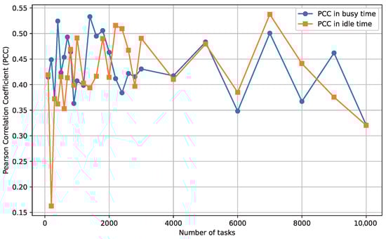
Figure 3. Positive correlation between FTG and SPD for Alibaba workflows with 50 GPUs.

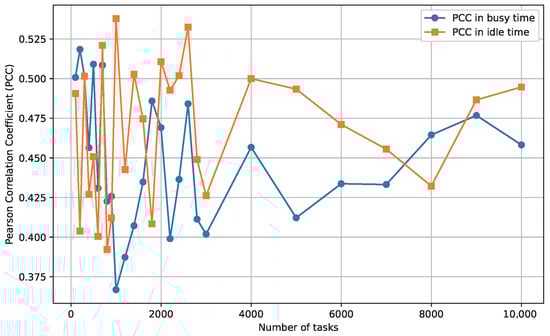
Figure 4. Positive correlation between FTG and SPD for Alibaba workflows with 500 GPUs.

We acknowledge that the average PCC of 0.4603 reflects moderate rather than strong linear correlation (where PCC > 0.7 is conventionally considered strong). However, in complex DAG scheduling under resource contention and precedence constraints, there may not exist perfect linearity and consistent directional alignment is of more practical significance: SPD and FTG monotonically co-vary across all tested conditions. To further validate this non-parametric robustness, we supplement SPD and FTG with Spearman’s rank correlation coefficient ($\rho$), which measures monotonicity without the assumption on linearity.

Table 2 reports Spearman’s $\rho$ for the same experimental configurations. Values range from 0.49 to 0.55 with mean = 0.52 and variance = 0.004, consistently higher than PCC and uniformly positive, confirming that the relationship between SPD and FTG is even stronger than linear trends. This is expected because structural divergence SPD influences makespan FTG through cumulative, nonlinear dependency chains, precisely the regime where rank-based metrics outperform Pearson’s. Critically, no configuration yields negative $\rho$, and the gap $\rho >\mathrm{PCC}$ holds in 92% of the cases, reinforcing that SPD provides reliable monotonic guidance even when linear fit is moderate. In optimization contexts such as WORL-RTGS, this ensures that minimizing SPD would reduce FTG on average. Edge cases with lower PCC (e.g., 0.386) still yield $\rho >0.41$, preserving directivity.

Table 2. Spearman’s $\rho$ between $\mathit{SPD}$ and $\mathit{FTG}$.

System	Scale	PCC	Spearman $\mathit{\rho }$
Busy	Small	0.439	0.489
Busy	Medium	0.462	0.536
Busy	Large	0.455	0.501
Idle	Small	0.458	0.528
Idle	Medium	0.466	0.552
Idle	Large	0.462	0.514

Synthetic Workload Experiments. The experimental analysis with synthetically generated workloads, also divided into busy and idle states. GPU resource usage is sampled in the same ranges as in the real-world experiments. We simulate the same six cluster environments, with job scales and node counts as previously described. Execution times for jobs are sampled from normal distributions: $N(10, 2^2)$ for small-scale, $N(20, 4^2)$ for medium-scale, and $N(30, 6^2)$ for large-scale jobs. DAG topologies are generated using the Erdos–Rényi model [45], with the average in-degree/out-degree set to either 1 or 3, resulting in 54 workloads in total: 27 with degree 1 and 27 with degree 3. For each combination of system state, job scale, GPU count, and average degree, we perform 1000 independent repetitions. In each repetition, two scheduling plans, ${\mathcal{S}}_1$ and ${\mathcal{S}}_2$, are randomly created, and $\mathit{SPD}$ and $\mathit{FTG}$ are computed. The $(\mathit{SPD},\mathit{FTG})$ pairs are recorded for correlation analysis, and the PCC is computed for each combination to measure the correlation strength between $\mathit{SPD}$ and $\mathit{FTG}$.

Table 3 reports the PCC values between $\mathit{SPD}$ and $\mathit{FTG}$ under synthetic workloads across different system states, job scales, GPU counts, and average in-degree/out-degree. Overall, the results demonstrate a consistently positive correlation, with PCC values ranging approximately from 0.39 to 0.55. Stronger correlations are observed for medium and large workloads in the busy state, especially when the correlation degree is 3 (e.g., 0.550 at 20 GPUs and 0.534 at 200 GPUs). In the idle state, small workloads exhibit greater variability, while medium and large workloads remain relatively stable, often exceeding 0.45 and reaching above 0.54 in several cases. Figure 5 and Figure 6 further show the positive trend, showing consistent correlation of 50 GPUs and 500 GPUs. These PCC values indicate a moderate correlation strength, aligning well with benchmarks in the scheduling literature where proxy metrics for makespan (e.g., load imbalance or resource utilization) typically yield PCCs in the range of 0.3–0.6 [43,44], particularly in heterogeneous or variable-degree topologies. In our case, the slightly higher PCCs for $d=3$ (e.g., up to 0.550) underscore SPD’s enhanced predictiveness in denser graphs, where inter-task dependencies amplify load-makespan sensitivity, ideal for our proxy’s role in WORL-RTGS, as it enables reliable indirect minimization of FTG amid topological variability.

Table 3. PCC for $\mathit{SPD}$ and $\mathit{FTG}$ on synthetic workloads.

System State	Job Scale	Degree	10 GPUs	20 GPUs	50 GPUs	100 GPUs	200 GPUs	500 GPUs
Busy	Small	1	0.473	0.489	0.456	0.438	0.439	0.434
		3	0.471	0.442	0.474	0.388	0.466	0.411
	Medium	1	0.416	0.418	0.477	0.434	0.491	0.396
		3	0.538	0.550	0.487	0.391	0.469	0.412
	Large	1	0.423	0.433	0.488	0.503	0.514	0.413
		3	0.538	0.549	0.495	0.396	0.534	0.424
Idle	Small	1	0.533	0.397	0.438	0.513	0.409	0.429
		3	0.435	0.447	0.476	0.430	0.402	0.466
	Medium	1	0.447	0.476	0.490	0.544	0.540	0.404
		3	0.503	0.522	0.458	0.438	0.512	0.438
	Large	1	0.404	0.551	0.465	0.499	0.536	0.422
		3	0.522	0.431	0.462	0.403	0.407	0.440

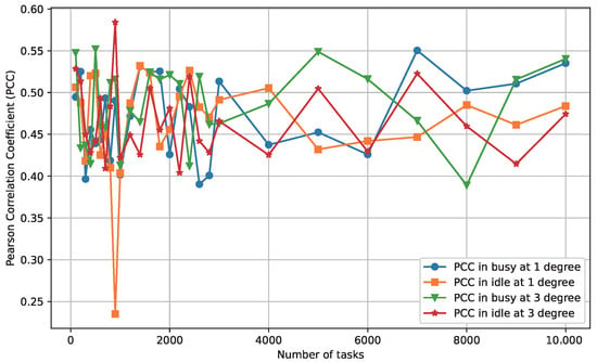
Figure 5. Positive correlation between FTG and SPD for synthetic workflows with 50 GPUs.

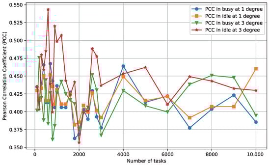
Figure 6. Positive correlation between FTG and SPD for synthetic workflows with 500 GPUs.

As in the real-world data, we compute Spearman’s $\rho$ for synthetic workloads. Across all 108 configurations, $\rho$ ranges from 0.42 to 0.59 with mean = 0.508 and variance = 0.004, again outperforming PCC and uniformly positive. The improvement is most pronounced in high-degree ($d=3$) topologies, where dependency chains amplify effects (e.g., $\rho =0.58$ vs. PCC = 0.550 at 20 GPUs, medium scale, busy state). This further validates SPD’s robustness as a proxy in topologically complex scenarios.

Furthermore, the positive correlation observed in Figure 3, Figure 4, Figure 5 and Figure 6 has profound implications: it empirically substantiates that greater structural divergence in scheduling plans (SPD) reliably predicts larger makespan disparities (FTG), enabling SPD to steer search toward balanced, low-makespan solutions without exhaustive FTG evaluations. This not only accelerates convergence in metaheuristic frameworks but also enhances load balancing, as higher SPD correlates with imbalance-induced delays, directly tying to energy efficiency and SLA compliance on GPU clusters.

The results shown in the experiments of real-world data and synthetic workloads confirm a persistent positive correlation between $FTG$ and $SPD$ across varying conditions. In all cases, the PCC value remains above zero. From a statistical perspective, the PCC values ranging from 0.16 to 0.57 with the average of 0.4603 and variance around 0.003 suggest a consistent trend: as $\mathit{FTG}$ increases, $\mathit{SPD}$ tends to increase as well. These experiments clearly illustrate the increasing trend of $\mathit{SPD}$ with larger values of $\mathit{FTG}$. This persistent positive correlation, spanning workload scale, topology, cluster size, and utilization, validates SPD as a reliable proxy for FTG. The moderate PCC strength (mean 0.46) is reasonable for DAG scheduling problems, where exact linearity may not exist due to precedence constraints and resource heterogeneity [43,44]; instead, it ensures directional guidance for optimization, reducing makespan by aligning structural adjustments with performance gaps. Notably, the absence of negative correlations across diverse setups and the low variance (0.003) make SPD a computationally tractable surrogate in iterative algorithms such as WORL-RTGS. We report global Spearman’s $\rho =0.51\pm 0.004$, reinforcing stability and predictability. In WORL-RTGS, we exploit this relationship to indirectly optimize makespan by minimizing SPD via differentiable, structural updates (Section 4.3). The data and code used to generate these visualizations are publicly available in our GitHub repository (https://github.com/AIprinter/WORL-RTGS.git, accessed on 6 November 2025).  This observed correlation plays a crucial role in our algorithm design. It provides theoretical and empirical support for using $\mathit{SPD}$ as a proxy to indirectly control and optimize $\mathit{FTG}$, thereby improving the efficiency of our scheduling strategy.

4.3. Whale Optimization and Reinforcement Learning-Based Running Time Gap Strategy

We design WORL-RTGS by integrating the WOA with a Deep Reinforcement Learning (DRL) framework. WOA is a nature-inspired meta-heuristic optimization algorithm introduced by Seyedali et al. [7] in 2016, modeled on the unique hunting behavior of humpback whales [46].

In the context of WORL-RTGS, each humpback whale metaphorically represents a candidate scheduling plan. This plan is encoded as an n-dimensional vector, where each dimension specifies the GPU assigned to a corresponding task node. A population of whales is maintained across iterations, with each whale representing a different scheduling plan. Following the core principles of WOA, the optimization process in WORL-RTGS is divided into three phases. Encircling Prey phase simulates the convergence towards an optimal solution, Spiral Bubble-Net Feeding Maneuver balances exploration and exploitation through a logarithmic spiral, and Search for Prey phase diversifies the search space by moving whales randomly. In each iteration, every whale updates its position by executing one of these three directions. However, the traditional WOA mechanism is insufficient for accurately determining the position matrix of a new whale when applied to complex task scheduling problems, especially in high-dimensional GPU assignment spaces. To overcome this limitation, WORL-RTGS integrates a Double Deep Q-Network (DDQN) module within the DRL framework. Based on the direction selected by WOA, the DDQN is responsible for predicting the next-step position matrix for each whale, thereby enhancing the quality and precision of the scheduling plan evolution.

4.3.1. Encircling Prey

Humpback whales are able to detect prey and move around it. In WORL-RTGS, the prey’s position is analogous to the Optimal Scheduling Plan (OSP). Since the exact OSP is unknown beforehand, the algorithm instead designates the best available scheduling plan at each step as the target prey, represented by the leading whale. Once this leader is identified, the remaining whales adjust their positions in relation to it, which is expressed mathematically as

$$\begin{array}{c}D=\left|C·{\mathcal{S}}^{\ast }\left(k\right)-\mathcal{S}\left(k\right)\right|,\end{array}$$

(31)

$$\begin{array}{c}\mathcal{S}\left(k+1\right)={\mathcal{S}}^{\ast }\left(k\right)-A·D,\end{array}$$

(32)

where k denotes the iteration index, while A and C are coefficients obtained from Equations (33) and (34). The term ${\mathcal{S}}^{\ast }\left(k\right)$ represents the leader’s position, i.e., the best scheduling plan in iteration k. Each whale in the population is represented by $\mathcal{S}\left(k\right)$, and its updated position in the next iteration is given by $\mathcal{S}(k+1)$. The symbol $| |$ indicates element-wise absolute values, and the operator · refers to element-wise multiplication. The distance between a whale $\mathcal{S}\left(k\right)$ and the leader ${\mathcal{S}}^{\ast }\left(k\right)$ is expressed as D. The definitions of A and C are provided below:

$$\begin{array}{c}A=2a^{\prime }·r^{\prime }-a^{\prime },\end{array}$$

(33)

$$\begin{array}{c}C=2·r^{\prime }-1,\end{array}$$

(34)

$$\begin{array}{c}{a}^{\prime }=2·\left(1-{\displaystyle \frac{k}{k_{\max }}}\right),\end{array}$$

(35)

where $r^{\prime }$ is a random value uniformly sampled from the interval $[0, 1]$. The parameter $r^{\prime }$ introduces stochasticity into both A and C, ensuring population diversity and preventing premature convergence. Its value in $[0, 1]$ represents the normalized probability range for random behavior: $r^{\prime }=0$ corresponds to no influence from the leader (pure exploration), whereas $r^{\prime }=1$ enforces complete attraction toward the leader (pure exploitation). This probabilistic modulation helps balance the two phases during optimization. The coefficient $a^{\prime }$ controls the exploration–exploitation transition. As Equation (35) shows, $a^{\prime }$ decreases linearly from 2 to 0 as the iteration index k increases, meaning that early iterations favor exploration (larger A range) and later iterations emphasize exploitation (smaller A). Consequently, A is confined to the range $[-a^{\prime },a^{\prime }]$, gradually shrinking to zero as convergence progresses. $k_{\max }$ denotes the maximum number of iterations and governs the temporal decay of $a^{\prime }$. Together, $(a^{\prime },r^{\prime })$ dynamically adjust the search pressure toward the best scheduling plan ${\mathcal{S}}^{\ast }\left(k\right)$.

In practice, Equation (31) can measure the actual distance between humpbacks, but applying it directly to scheduling plans is not meaningful. Each dimension of a plan corresponds to a GPU index, and subtracting one index from another provides no useful interpretation. To resolve this, we introduce $FTG$, defined in Equation (25), as a metric for quantifying differences between humpbacks. However, $FTG$ by itself is insufficient for directly producing new scheduling plans. To overcome this limitation, we leverage its positive correlation with $\mathit{SPD}$, as discussed in Section 4.2. By translating $FTG$ into $\mathit{SPD}$, we derive a more actionable metric that facilitates the generation of new humpback positions—corresponding to scheduling plans—throughout the iterative procedure.

It is not feasible to directly generate the next-step humpback whale location, $\mathcal{S}(t+1)$, using Equation (32) based solely on a given value of $\mathit{FTG}$, as computed from Equation (25). The challenge stems from the fact that $\mathit{FTG}$ is a single scalar capturing only the absolute gap in final finish times, while scheduling plans are inherently high-dimensional vectors. As a result, $\mathit{FTG}$ lacks the necessary structure and dimensionality to guide the generation of a new scheduling plan vector directly. To overcome this challenge, we must find a function that not only reflects the behavior of $\mathit{FTG}$ but also supports extension into a multidimensional space consistent with the representation of scheduling plans. This is where our earlier analysis proves useful: we have observed a medium positive correlation between $\mathit{FTG}$ and $\mathit{SPD}$ in Section 4.2, meaning that as the $\mathit{SPD}$ between two scheduling plans increases, the corresponding $\mathit{FTG}$ also tends to increase. This correlation enables us to indirectly control $\mathit{FTG}$ by manipulating $\mathit{SPD}$. Therefore, in the optimization process, we replace the original abstract distance term D in Equation (32) with $\mathit{SPD}$ to guide the humpback’s movement. Unlike $\mathit{FTG}$, $\mathit{SPD}$ is computable based on the structural differences between scheduling plans and can be naturally expanded to a higher dimensions. This allows us to use $\mathit{SPD}$ not only as a proxy for $\mathit{FTG}$ but also as a foundation for deriving new, high-dimensional scheduling plans through Reinforcement Learning-driven methods.

The next position of a humpback whale, $\mathcal{S}(k+1)$, is obtained by first deriving a set of target values, referred to as $\mathit{hope}\left(l_i\right)$. Each $\mathit{hope}\left(l_i\right)$ represents the expected workload which is the total execution time of the GPU that task node $l_i$ is expected to be assigned to in the upcoming scheduling plan $\mathcal{S}(k+1)$. Formally, this is expressed as

$$\begin{array}{c}\hfill \mathit{hope}\left(l_i\right)=loa{d}_{\mathcal{S}(k+1)}\left(map\left(l_i\right)\right),\end{array}$$

(36)

where $map\left(l_i\right)$ indicates the GPU to which task node $l_i$ is mapped, and $loa{d}_{\mathcal{S}(k+1)}$ computes the total execution time of tasks assigned to that GPU under the new plan.

To construct this list of hope values for all task nodes $l_i\in L$, we rely on both the leader whale’s location and the current whale’s position in iteration k. Specifically, $lead\left(l_i\right)$ denotes the current load on the GPU handling task node $l_i$ in the leader whale’s scheduling plan ${\mathcal{S}}^{\ast }\left(k\right)$:

$$\begin{array}{cc}\hfill lead\left(l_i\right)& =loa{d}_{{{\mathcal{S}}^{\ast }}_{\left(k\right)}}\left(map\left(l_i\right)\right),\hfill \end{array}$$

(37)

$\mathit{curr}\left(l_i\right)$ represents the current load on the GPU handling $l_i$ in the given humpback’s current location $\mathcal{S}\left(k\right)$:

$$\begin{array}{c}\hfill \mathit{curr}\left(l_i\right)=loa{d}_{\mathcal{S}\left(k\right)}\left(map\left(l_i\right)\right).\end{array}$$

(38)

With both $lead\left(l_i\right)$ and $\mathit{curr}\left(l_i\right)$ known, the algorithm derives $\mathit{hope}\left(l_i\right)$ based on the relative influence of the leader and current humpback states guided by the coefficients defined in the WOA mechanism. This hope value list then serves as a basis for reassigning task nodes in order to construct the whale’s next-step scheduling plan $\mathcal{S}(k+1)$.

Substituting Equation (31) into Equation (32) and comparing with Equation (25), we obtain the following:

$$\begin{array}{cc}\hfill {\mathcal{S}}^{\ast }\left(k\right)-\mathcal{S}(k+1)& =A·\left|C·{\mathcal{S}}^{\ast }\left(k\right)-\mathcal{S}\left(k\right)\right|,\hfill \\ \hfill \mathit{FTG}\left({\mathcal{S}}^{\ast }\left(k\right),\mathcal{S}(k+1)\right)& =A·\mathit{FTG}\left({\mathcal{S}}^{\ast }\left(k\right),\mathcal{S}\left(k\right)\right).\hfill \end{array}$$

(39)

Here, D is substituted with $\mathit{FTG}$ to quantify the gap between two scheduling plans. As shown in Equation (39), the gap between the leader whale and its follower in the next step is scaled by factor A. During this stage, the randomness term C is omitted; assigning $C=1$ effectively removes stochasticity and ensures the leader humpback’s position remains deterministic.

Since Section 4.2 shows a positive correlation between $\mathit{FTG}$ and $\mathit{SPD}$, we suggest employing $\mathit{SPD}$ as a substitute for $\mathit{FTG}$. By making this substitution in Equation (39), we bridge the distance with a more interpretable and extendable metric in multidimensional scheduling space. Thus, the distance between the leader’s load distribution and the hope distribution in the next-step schedule can be expressed as

$$\begin{array}{cc}\hfill {\displaystyle \frac{1}{n}}\sum _{l_i\in L}\left|lead\left(l_i\right)-\mathit{hope}\left(l_i\right)\right|& ={\displaystyle \frac{A}{n}}\sum _{l_i\in L}\left|lead\left(l_i\right)-\mathit{curr}\left(l_i\right)\right|,\hfill \end{array}$$

(40)

$$\begin{array}{cc}\hfill \sum _{l_i\in L}\left|lead\left(l_i\right)-\mathit{hope}\left(l_i\right)\right|& =\sum _{l_i\in L}A·\left|lead\left(l_i\right)-\mathit{curr}\left(l_i\right)\right|.\hfill \end{array}$$

(41)

To derive the above expressions, we make a simplifying assumption: for each task node $l_i$, the corresponding terms on both sides of the equation are equal, that is

$$\begin{array}{cc}\hfill \left|lead\left(l_i\right)-\mathit{hope}\left(l_i\right)\right|& =A·\left|lead\left(l_i\right)-\mathit{curr}\left(l_i\right)\right|.\hfill \end{array}$$

(42)

Under this assumption, the hope load for each GPU node at the next position $\mathcal{S}(k+1)$ can be calculated through the following transformation:

$$\begin{array}{cc}\hfill lead\left(l_i\right)-\mathit{hope}\left(l_i\right)& =\pm A·\left(lead\left(l_i\right)-\mathit{curr}\left(l_i\right)\right),\hfill \\ \hfill \mathit{hope}\left(l_i\right)=lead\left(l_i\right)& \pm A·\left(lead\left(l_i\right)-\mathit{curr}\left(l_i\right)\right).\hfill \end{array}$$

(43)

Equation (43) expresses the estimated load on the GPU hosting task node $l_i$ at the humpback whale’s next position. It is calculated based on a weighted difference between the leader whale’s load and the current whale’s load, scaled by the factor A. The ± sign introduces a bifurcation in movement direction, which aligns with the behavior modeled by the WOA algorithm enabling the search to either approach or diverge from the leader, depending on the optimization dynamics in a given iteration. WORL-RTGS feeds the value of $\mathit{hope}\left(l_i\right)$ from Equation (43) into the DDQN module detailed in Section 4.3.4, which then determines the next humpback position according to the optimization objective.

In WORL-RTGS, every humpback whale chooses a unique direction for movement in each iteration. For each selected path, a distinct derivation process is applied to assess the computational demand on the GPU hosting each task node $l_i$ at the whale’s anticipated next location. For instance, in the Encircling Prey phase, this estimation is formulated in Equation (43), which provides the predicted load values referred to as hope values, based on the current and leader positions. In the subsequent sections, namely Section 4.3.2 and Section 4.3.3, we apply a similar derivation methodology to the other two behavioral strategies: Bubble-Net Attacking Method and Search for Prey. These derivations likewise yield a list of hope values tailored to each phase, enabling us to generate updated scheduling plans that reflect the selected movement strategy within the WOA-inspired optimization framework.

4.3.2. Bubble-Net Feeding Strategy (Exploitation Phase)

Humpback whales employ a distinctive hunting technique known as Bubble-Net Feeding [47]. They submerge approximately 12 m, then generate bubbles along a path resembling a ‘9’ to encircle a school of fish, ascending toward their target. This Bubble-Net Feeding behavior comprises two key mechanisms: a shrinking encirclement process and a spiral position update.

Shrinking encirclement process. In Equation (32), the coefficient A is randomly generated from the interval $\left[-a,a\right]$, with a decreasing linearly as the iteration index k grows. Consequently, the absolute value of A gradually reduces over the course of the iterations. This gradual reduction causes the search area around the the leader solution to contract progressively. In the context of the Encircling Prey phase, this mechanism reflects the humpback whale’s strategy of narrowing its focus and moving closer to the optimal solution as the optimization progresses. The shrinking encirclement helps guide the algorithm toward exploitation by reducing randomness and encouraging convergence in the later stages of the search process.

Spiral position update. Seyedali et al. [7] proposed a spiral equation to emulate the distinctive helical motion of humpback whales. The procedure first measures the distance between a whale at $\mathcal{S}\left(k\right)$ and the current leader at ${\mathcal{S}}^{\ast }\left(k\right)$. Based on this distance, a new position along a spiral path between $\mathcal{S}\left(k\right)$ and ${\mathcal{S}}^{\ast }\left(k\right)$ is computed using the following formulation:

$$\mathcal{S}\left(k+1\right)=D^{\prime }·e^{bl}·\cos \left(2\pi l\right)+{\mathcal{S}}^{\ast }\left(k\right),$$

(44)

where $D^{\prime }=\left|{\mathcal{S}}^{\ast }\left(k\right)-\mathcal{S}\left(k\right)\right|$ represents the distance between the whale’s current position and that of the leader, b is a constant parameter, and l is a random value sampled from the interval $[-1, 1]$. The random variable $l\in [-1, 1]$ controls the direction and amplitude of the spiral motion. Values of l close to $-1$ produce outward spirals (encouraging exploration), while values near 1 generate inward spirals that contract toward the leader (favoring exploitation). Sampling l symmetrically around zero allows the algorithm to maintain a balanced probabilistic tendency between expansion and contraction around the current best solution.

As in the Encircling Prey strategy, the Spiral Bubble-Net Movement determines the whale’s next position $\mathcal{S}(k+1)$ by first estimating the hope load on the GPU assigned to task node $l_i$ at that location. Using a derivation approach analogous to that in the encircling phase, we obtain the following expression for the hope value:

$$\begin{array}{cc}\hfill \mathit{hope}\left(l_i\right)& =lead\left(l_i\right)\pm A^{\prime }·\left(lead\left(l_i\right)-\mathit{curr}\left(l_i\right)\right),\hfill \end{array}$$

(45)

$$\begin{array}{cc}\hfill A^{\prime }& =e^{bl}·\cos \left(2\pi l\right).\hfill \end{array}$$

(46)

Humpbacks reduce the circle while following a spiral trajectory at the same time. To replicate this dual behavior, a random variable $p\in [0, 1]$ is introduced to decide the movement pattern. If $p\le 0.5$, the whale updates its position using the shrinking-encircling mechanism; otherwise, the spiral updating rule is applied as follows:

$$\mathit{hope}\left(l_i\right)=\left\{\begin{array}{c}lead\left(l_i\right)\pm A·\left(lead\left(l_i\right)-\mathit{curr}\left(l_i\right)\right),p⩽0.5\hfill \\ lead\left(l_i\right)\pm A^{\prime }·\left(lead\left(l_i\right)-\mathit{curr}\left(l_i\right)\right),p>0.5.\hfill \end{array}\right.$$

(47)

4.3.3. Searching for Prey (Exploration Phase)

In natural hunting scenarios, humpback whales know the prey’s location and head straight toward it. However, in the context of discovering a suboptimal scheduling plan, whales in WORL-RTGS are not always guaranteed to converge on a globally optimal solution. Instead, they may become trapped in a local optimum by repeatedly moving toward a currently best-known solution.

To enhance global exploration and avoid local optima, WORL-RTGS adopts a strategy where a humpback whale is forced to explore new regions of the solution space when $\left|A\right|>1$. Under this condition, the current leader whale is no longer followed. Instead, a random whale ${\mathcal{S}}_{rand}$ is selected to act as a temporary guide, and the current whale at position $\mathcal{S}\left(k\right)$ is repelled from this randomly chosen whale. This mechanism increases diversity in the population and encourages exploration of unvisited scheduling plans. The corresponding position update rule is given by

$$\begin{array}{c}\hfill \mathcal{S}\left(k+1\right)={\mathcal{S}}_{rand}-A·D,\end{array}$$

(48)

$$\begin{array}{c}\hfill D=\left|C·{\mathcal{S}}_{rand}-\mathcal{S}\left(k\right)\right|,\end{array}$$

(49)

where ${\mathcal{S}}_{rand}$ represents the scheduling plan of a randomly chosen whale, while D is the distance to this whale from the current whale, scaled by the random factor C.

To derive the expected workload which is the hope value on the GPU that hosts task node $l_i$ at the next-step location ${\mathcal{S}}_{\left(k+1\right)}$, we apply the same transformation used in other movement strategies. The resulting expression is

$$\begin{array}{cc}\hfill \mathit{hope}\left(l_i\right)& =rand\left(l_i\right)\pm A·\left(rand\left(l_i\right)-\mathit{curr}\left(l_i\right)\right),\hfill \end{array}$$

(50)

where $rand\left(l_i\right)=loa{d}_{{\mathcal{S}}_{rand}}\left(\mathit{map}\left(l_i\right)\right)$ is the current total execution time of all task nodes mapped to the GPU processing $l_i$ in the randomly selected whale. This equation allows WORL-RTGS to estimate the updated task distribution under the exploration-driven movement and facilitates the generation of new scheduling candidates with greater diversity.

Having introduced the three behavioral mechanisms of the humpback whale: Encircling Prey, Bubble-Net Attacking, and Search for Prey, we have derived three corresponding sets of target values, denoted as $\left\{\mathit{hope}\left(l_i\right)|l_i\in L\right\}$. Each set represents the desired workload outcomes for task nodes under one of the three movement strategies, guiding how the whale (i.e., the scheduling plan) should evolve in the next iteration. The next step is to translate these hope values into a concrete next-step scheduling plan, i.e., the whale’s updated position. To achieve this, the WORL-RTGS algorithm employs a Double Deep Q-Network (DDQN) framework. The DDQN is used to generate a scheduling plan that aligns as closely as possible with the desired workload distribution specified in the corresponding $\mathit{hope}\left(l_i\right)$ list, thereby guiding the whale or scheduling plan toward more optimal solutions in a structured and adaptive manner.

4.3.4. DDQN-Based Whale Position Generation

To generate an optimized scheduling plan $\mathcal{S}(k+1)$, we design a Double Deep Q-Network (DDQN) module that predicts the optimal GPU assignment for each task node $l_i$ based on its expected workload, denoted as $\mathit{hope}\left(l_i\right)$. The DDQN agent is trained to learn a mapping strategy that minimizes the deviation between the actual and expected GPU workloads, thereby enhancing scheduling efficiency in high-dimensional task allocation scenarios. The corresponding Markov Decision Process (MDP) is defined as follows.

• State Space $\mathrm{S}$:

Each state $s\left(l_i\right)$ characterizes the scheduling environment of task node $l_i$ and includes the following components: the index of the current task node $l_i$; the expected workload vector ${\overrightarrow{Lis}t}_{hope}\in {\mathbb{R}}^n$, where n denotes the total number of task nodes, and each entry corresponds to the desired total load on the GPU to which $l_i$ is expected to be assigned; the computational workload vector $\overrightarrow{W}\in {\mathbb{R}}^n$ for all task nodes (e.g., measured in FLOPs); and the current GPU load vector ${L\overrightarrow{oa}d}_{curr}\in {\mathbb{R}}^m$, where m is the number of GPUs. Thus, each state is represented as

$$s\left(l_i\right)=\left[l_i,{\overrightarrow{Lis}t}_{hope},\overrightarrow{W},{L\overrightarrow{oa}d}_{curr}\right].$$

(51)

• Action Space $\mathcal{A}$:

The action space consists of all available GPUs:

$$\mathcal{A}=\{GP{U}_1,GP{U}_2,\dots ,GP{U}_m\}.$$

(52)

Each action $a\in \mathcal{A}$ corresponds to assigning task node $l_i$ to a specific GPU.

• Reward Function $\mathcal{R}(s,a)$:

The reward function encourages the agent to minimize the deviation between the predicted and desired GPU workloads:

$$\mathcal{R}(s,a)=-\left|\mathrm{hope}\left(l_i\right)-{\mathrm{pred}\_\mathrm{load}}_a\left(l_i\right)\right|.$$

(53)

Here, ${\mathrm{pred}\_\mathrm{load}}_a\left(l_i\right)$ denotes the predicted load on GPU a after assigning task node $l_i$ to it. The closer this predicted load is to the desired workload value $\mathrm{hope}\left(l_i\right)$, the higher (i.e., less negative) the reward.

• Training Objective:

The training objective is to derive a scheduling policy that reduces the overall Load Deviation ($LoD$) once all task nodes have been allocated. The $LoD$ is defined as

$$\begin{array}{c}\hfill LoD=\sum _{i=1}^n|\mathrm{hope}\left(l_i\right)-{\mathrm{load}}_{\mathcal{S}(k+1)}\left(map\left(l_i\right)\right)|,\end{array}$$

(54)

where ${\mathrm{load}}_{\mathcal{S}(k+1)}\left(map\left(l_i\right)\right)$ denotes the total runtime of all tasks assigned to the same GPU as $l_i$ in the final plan, and $\mathrm{hope}\left(l_i\right)$ represents the expected workload prior to scheduling.

• DDQN Architecture:

The DDQN module is implemented using a lightweight multilayer perceptron (MLP) architecture. The network receives a state vector $s\left(l_i\right)\in {\mathbb{R}}^{2n+m+1}$ as input, which encodes the scheduling environment of the current task node. The output is a Q-value vector $Q(s,a)\in {\mathbb{R}}^m$, where each element corresponds to the estimated cumulative reward of assigning task node $l_i$ to one of the m available GPUs. The network consists of an input layer of size $2n+m+1$. This is followed by two hidden layers containing 128 and 64 units, respectively, each using the ReLU activation function. The final output layer has m units and uses a linear activation to produce Q-values for each possible GPU assignment.

During training, we employ experience replay and the Double DQN target update strategy to stabilize learning. The Q-value update is computed as

$$y=r+\gamma ·Q_{\mathrm{target}}(s^{\prime },\arg \underset{a}{\max }{Q}_{\mathrm{online}}(s^{\prime },a)),$$

with the corresponding loss function defined as

$$\mathcal{L}={\left(y-Q_{\mathrm{online}}(s,a)\right)}^2.$$

To mitigate overestimation bias, the parameters of the target network are periodically synchronized with those of the online network.

The pseudocode of the DDQN-based whale position generation method is presented in Algorithm 1. This method is applied in conjunction with the three behavioral mechanisms of the humpback whale: Encircling Prey, Bubble-Net Attacking, and Search for Prey, each of which yields a corresponding set of target values, denoted as $\left\{\mathit{hope}\left(l_i\right)\mid l_i\in L\right\}$. The complete pseudocode of the overall WORL-RTGS algorithm is provided in Algorithm 2. We begin by presenting the pseudocode of Algorithm 1, followed by the full process of the WORL-RTGS algorithm as shown in Algorithm 2. Algorithm 1 presents the DDQN-based task-to-GPU scheduling method. In each training episode, task nodes are scheduled sequentially according to a topological order. For each task node, the current state is constructed and used as input to the online Q-network to select the GPU with the highest predicted Q-value. The selected action is applied by assigning the task to the chosen GPU and updating the current load. A reward is computed based on the deviation between the expected and predicted GPU load, and the transition tuple $(s,a,r,s^{\prime })$ is stored in the replay buffer. Mini-batches drawn from the buffer are employed to update the online network through Q-learning, with target Q-values computed using the Double DQN approach. The target network is synchronized with the online network at regular intervals. After training, the learned Q-network is used to generate the final scheduling plan $\mathcal{S}(k+1)$. Algorithm 2 outlines the integrated optimization procedure of the WORL-RTGS algorithm, which combines the Whale Optimization Algorithm (WOA) with a DDQN-based scheduling module. The algorithm begins by initializing a population of humpback whales and evaluating their fitness values using Equation (17). The best-performing whale is selected as the current leader. At each iteration, whale positions are updated according to one of three behaviors: Encircling Prey, Searching for Prey, or Spiral Bubble-Net Attack, determined by the randomly chosen control parameters r and p. For each behavior, a corresponding hope value list ${\overrightarrow{Lis}t}_{hope}$ is computed, and the DDQN module as Algorithm 1 is invoked to guide the position update. After all whales are updated, their fitness values are re-evaluated and the leader is updated accordingly. The process continues until the maximum iteration limit is reached, at which point the optimal solution ${\mathcal{S}}^{\ast }$ is delivered. As iterations progress, the magnitude of $\left|A\right|$ steadily declines from 2 to 0, facilitating a shift from exploration to exploitation. In each cycle, WORL-RTGS chooses between a spiral or circular trajectory based on a randomly determined parameter p. Once a humpback whale selects its movement pattern, a set of hope values $\left\{\mathit{hope}\left(l_i\right)\mid l_i\in L\right\}$ is computed. Guided by a Q-network, a new whale position is established by fulfilling these hope values. Successful fulfillment of the hope values ensures that the $\mathit{FTG}$ metric is also met, owing to its positive correlation with $\mathit{SPD}$, as discussed in Section 4.2. For reference, the primary parameters utilized in the algorithm are outlined in Table 4.

Algorithm 1 DDQN-Based Task-to-GPU Scheduling Algorithm.

1: Input: Task set $L=\{l_1,l_2,\dots ,l_n\}$, initial GPU loads ${L\overrightarrow{oa}d}_{curr}$, hope vector ${\overrightarrow{Lis}t}_{hope}$ 2: Output: Scheduling plan $\mathcal{S}(k+1)$ 3: Initialize $Q_{\mathrm{online}}$, $Q_{\mathrm{target}}$, and replay buffer $\mathcal{D}$ 4: for episode = 1 to $N_{\mathrm{episodes}}$ do 5:       for each task node $l_i$ in topological order do 6:             Construct state s 7:             $a\leftarrow \arg \max Q_{\mathrm{online}}(s,a)$ 8:             Assign $l_i$ to GPU a, update ${L\overrightarrow{oa}d}_{curr}$ 9:             Compute reward r 10:           Construct next state $s^{\prime }$ 11:           Store $(s,a,r,s^{\prime })$ in $\mathcal{D}$ 12:           Sample batch from $\mathcal{D}$ 13:           for each $(s,a,r,s^{\prime })$ in batch do 14:                 $a^{\prime }\leftarrow \arg \max Q_{\mathrm{online}}(s^{\prime },a)$ 15:                 $y\leftarrow r+\gamma ·Q_{\mathrm{target}}(s^{\prime },a^{\prime })$ 16:                 Update $Q_{\mathrm{online}}$ with loss ${(y-Q_{\mathrm{online}}(s,a))}^2$ 17:           Periodically update $Q_{\mathrm{target}}$ 18: return Final scheduling plan $\mathcal{S}(k+1)$

Table 4. Notations and parameter descriptions used in the algorithm.

Parameter	Description
$\mathit{SPD}$	Distance measure between two scheduling plans
k	Current iteration index
$k_{\max }$	Maximum number of iterations
$loa{d}_{\mathcal{S}}\left(map\left(l\right)\right)$	Total execution time of tasks assigned to the GPU executing node l in plan $\mathcal{S}$
$\mathit{FTG}$	Gap in final finish time between two scheduling plans
${\mathcal{S}}^{\ast }$	Position of the leader whale
$\mathcal{S}\left(k\right)$	Whale’s position at iteration k
$r^{\prime },l$	Two random values
p	Random variable controlling spiral vs. circular movement
$A,C,a^{\prime },A^{\prime }$	Coefficients
$\mathrm{S}$	State space
$s\left(l_i\right)$	A state in state space $\mathrm{S}$
$l_i$	Index of the current task node
${\overrightarrow{Lis}t}_{hope}$	Expected workload for each task node
$\overrightarrow{W}$	Computational demands of all task nodes (e.g., FLOPs)
${L\overrightarrow{oa}d}_{curr}$	Current load on each GPU
$\overrightarrow{C}$	Computational capability of each GPU (e.g., TFLOPS)
$\mathcal{A}$	Action space
a	An action in action space $\mathcal{A}$
$\mathcal{R}(s,a)$	Reward function
${\mathrm{pred}\_\mathrm{load}}_a\left(l_i\right)$	The predicted load on GPU a after assigning task node $l_i$ to it
$LoD$	The Load Deviation, which is the training objective
$Q(s,a)$	A Q-value vector
$\mathcal{L}$	Loss function
$b^{\prime }$	Batch size used in the replay buffer during Q-network training
$N_{\mathrm{episodes}}$	Count of training episodes
$numHump$	Count of whales in the population
$numIter$	Total number of whale position update iterations

The overall computational complexity of the WORL-RTGS algorithm is determined by the interaction between the Whale Optimization loop and the DDQN-based scheduling procedure embedded within each iteration. In the DDQN-based whale next-position generation method Algorithm 1, let $b^{\prime }$ denote the batch size used in the replay buffer during training and n denote the number of task nodes. Let $N_{\mathrm{episodes}}$ denote the number of training episodes. For each episode, the algorithm iterates over all n task nodes. For each task node, it performs: state construction and action selection using the Q-network: $\mathcal{O}\left(m\right)$, where m is the number of GPUs; reward computation and buffer update: $\mathcal{O}\left(1\right)$; and backpropagation on the sampled batch of size $b^{\prime }$: $\mathcal{O}(b^{\prime }·m)$. Thus, the total complexity of the DDQN module per episode is $\mathcal{O}(n·(m+b^{\prime }·m))=\mathcal{O}(n·b^{\prime }·m)$, and the overall complexity across $N_{\mathrm{episodes}}$ episodes is ${\mathrm{Cost}}_{\mathrm{DDQN}}=\mathcal{O}(N_{\mathrm{episodes}}·n·b^{\prime }·m)$. In the WORL-RTGS optimization loop Algorithm 2, let $numHump$ denote the number of whales in the population, and $numIter$ the total number of optimization iterations. In each iteration, the algorithm evaluates and updates the position of each whale using one of three behavioral strategies. Each position update invokes the DDQN module once. Therefore, the total complexity of the WORL-RTGS algorithm is $\mathcal{O}(numIter·numHump·{\mathrm{Cos}\mathrm{t}}_{\mathrm{DDQN}})=\mathcal{O}(numIter·numHump·N_{\mathrm{episodes}}·n·b^{\prime }·m).$ This reflects the nested nature of the hybrid metaheuristic–learning framework, where each metaheuristic update is guided by a learned scheduling policy.

Algorithm 2 WORL-RTGS Integrated Optimization Procedure.

1: Input: Maximum number of iterations $numIter$; number of humpback whales $numHump$; 2: Randomly initialize the population of humpback whales ${\mathcal{S}}_i$, where $i=1,2,\dots ,numHump$; 3: Compute the fitness value ($FFT$) of each whale according to Equation (17); 4: Identify the whale with the smallest $FFT$ and assign it as the leader ${\mathcal{S}}^{\ast }$; 5: Initialize iteration counter: $k\leftarrow 0$; 6: while $k<numIter$ do 7:       for each whale in the population do 8:             Randomly generate control parameters r and p; 9:             Update the coefficient A using Equation (33); 10:           if $p<0.5$ then 11:                if $\left|A\right|<1$ then 12:                     Compute the hope value list ${\overrightarrow{Lis}t}_{hope}$ using Equation (43); 13:                     Update the whale position using the DDQN-based method Algorithm 1; 14:                else if $\left|A\right|\ge 1$ then 15:                     Randomly select a whale ${\mathcal{S}}_{rand}$ and assign it as ${\mathcal{S}}^{\ast }$; 16:                     Compute the hope value list ${\overrightarrow{Lis}t}_{hope}$ using Equation (50); 17:                     Update the whale position using the DDQN-based method Algorithm 1; 18:           else if $p\ge 0.5$ then 19:                Update A using the spiral equation: $A=e^{bl}·\cos \left(2\pi l\right)$; 20:                Compute the hope value list ${\overrightarrow{Lis}t}_{hope}$ using Equation (45); 21:                Update the whale position using the DDQN-based method Algorithm 1; 22:      Recalculate the $FFT$ for all whales; 23:      Update the leader ${\mathcal{S}}^{\ast }$ based on the best fitness; 24:      Increment iteration: $k\leftarrow k+1$; 25: Output: Final optimal solution ${\mathcal{S}}^{\ast }$;

The space complexity of the DDQN-based scheduler mainly consists of three parts: the parameters of the online and target Q-networks, the experience replay buffer, and auxiliary data structures for state and load tracking. Assuming an $L^{\prime }$-layer neural network with hidden dimension h, the space for network parameters is $\mathcal{O}(L^{\prime }·h^2)$. Since both $Q_{\mathrm{online}}$ and $Q_{\mathrm{target}}$ are maintained, the total becomes $\mathcal{O}(2L·h^2)$. The replay buffer stores $b^{\prime }$ experience tuples, each with state, action, reward, and next state, leading to space $\mathcal{O}(b^{\prime }·(2n+m+1))$, where $(2n+m+1)$ is the state vector dimension. Additionally, the scheduling plan and GPU load tracking introduce negligible overhead $\mathcal{O}(n+m)$. In total, the space complexity is $\mathcal{O}(L^{\prime }·h^2+b^{\prime }·(n+m))$.

5. Performance Evaluation

5.1. Experiment Setup

In this section, we first analyze the sensitivity of four key parameters: the number of training episodes $N_{\mathrm{episodes}}$, the discount factor $\gamma$, the maximum number of iterations $numIter$, and the spiral coefficient b. We then conduct comparative experiments between WORL-RTGS and five baseline scheduling algorithms, using both real-world workloads from the Alibaba Cluster Trace v2018 (https://github.com/alibaba/clusterdata, accessed on 6 November 2025) and synthetic DAG-structured workloads. The Alibaba Cluster Trace v2018, collected from Alibaba’s production environment, spans approximately 4000 machines over eight days. It provides DAG-structured workloads, machine status snapshots at each timestamp, and detailed execution logs. To cover short-, medium-, and long-duration workloads, we select jobs from the trace with roughly 100–1000 tasks in steps of 100 for small-scale workloads, 1200–3000 tasks in steps of 200 for medium-scale workloads, and 4000–10,000 tasks in steps of 1000 for large-scale workloads, noting that task counts are approximate. Our evaluation consists of four experimental sets based on DAG-structured workloads, examining system performance under both high-load and low-load server conditions.

The WORL-RTGS algorithm and all baseline scheduling methods are implemented in Java. Workload scheduling tests are executed on a cluster of nine local servers running Ubuntu 20.04.6 LTS with Java 1.8.0_191. Data processing and visualization of results are conducted using Python 3.14.0 on a Windows-based PC. All source code, datasets, and selected instance configurations are openly accessible on GitHub (https://github.com/AIprinter/WORL-RTGS.git, accessed on 6 November 2025).

5.2. Comparison Algorithms

• DRAS algorithm [29]: A hierarchical Deep Reinforcement Learning (DRL) framework designed for High-Performance Computing (HPC) clusters. It learns a dynamic scheduling policy via Deep Reinforcement Learning (RL), outperforming traditional heuristics by up to 45%.
• mDRL algorithm [32]: This approach leverages multi-agent Reinforcement Learning combined with graph neural networks to schedule deep learning jobs in large GPU clusters. The method focuses on minimizing job completion time by encoding cluster topology and modeling interference. It achieves over 20% improvements compared to stateless schedulers.
• MAGRL algorithm [31]: A topology-aware scheduling framework for large-scale GPU clusters. It uses multiple cooperative RL agents and a hierarchical graph neural network to model both intra-server and inter-scheduler structures. To handle limited feedback, MAGRL incorporates a learned interference model to predict co-location performance. Experiments show it reduces average job completion time by over 20%.
• RL-Hybrid algorithm [33]: This work models GPU cluster scheduling by explicitly accounting for network contention. A Reinforcement Learning agent learns to delay or reorder jobs to reduce network bottlenecks. Experiments show an 18.2% reduction in average job completion time and a 20.7% decrease in tail completion times compared to conventional schedulers.
• MIG+MPS algorithm [30]: Focusing on co-locating multiple tasks on a single GPU using NVIDIA’s MPS/MIG partitioning, this method employs deep RL to jointly optimize partition configuration and job co-location. It achieves up to 1.87× throughput improvement over traditional time-sharing scheduling.

We unify the notation across all the six algorithms to present a concise and consistent time and space complexity analysis. Let n denote the number of task nodes or jobs, m the number of available GPUs, $L^{\prime }$ the number of neural network layers, h the hidden layer width, $b^{\prime }$ the batch size or replay buffer size, $d_s$ the dimensionality of the input state vector, $d_a$ the dimensionality of the action vector, $N_{episode}$ the total number of training episodes, E the number of edges in a topology graph, and N the number of agents for multi-agent frameworks. For MAGRL, let $d_e$ be the GNN embedding dimension. For WORL-RTGS, let $numIter$ be the number of Whale Optimization iterations and $numHump$ the number of whales.

Although the theoretical time complexity of WORL-RTGS appears higher due to the presence of multiplicative constants such as $\mathit{numIter}$, $\mathit{numHump}$, $N_{episode}$, and $b^{\prime }$ as shown in Table 5, these values are typically small and fixed in practice. As a result, the actual runtime scaling of WORL-RTGS is primarily linear in the number of tasks n and GPUs m, making it computationally efficient in real-world deployments. In contrast, algorithms such as MAGRL and mDRL involve high-dimensional GNN embeddings $d_e$, large agent populations N, or complex state or action vectors with dimensionality $d_s$ and $d_a$, which can easily exceed hundreds of features. This leads to higher-order polynomial complexity terms like $\mathcal{O}\left(d_e^2\right)$ or $\mathcal{O}(b^{\prime }·(d_s+d_a))$, significantly increasing both computational and memory requirements. Therefore, from a practical perspective, WORL-RTGS achieves a balance by keeping model dimensionality compact and avoiding agent duplication, leading to competitive time and space efficiency in large-scale scheduling scenarios.

Table 5. Time and space complexity of six scheduling algorithms.

Algorithm	Time Complexity	Space Complexity
DRAS	$\mathcal{O}(N_{episode}·(n·d_s+b^{\prime }·L^{\prime }·h^2))$	$\mathcal{O}(L^{\prime }·h^2+b^{\prime }·d_s)$
mDRL	$\mathcal{O}(N·N_{episode}·(L^{\prime }·h^2+n))$	$\mathcal{O}(N·(L^{\prime }·h^2+b^{\prime }·d_s))$
MAGRL	$\mathcal{O}(N·L^{\prime }·E·d_e^2)$	$\mathcal{O}(N·L^{\prime }·d_e^2+b^{\prime }·(d_s+d_a))$
RL-Hybrid	$\mathcal{O}(L^{\prime }·h^2+n·m)$	$\mathcal{O}(L^{\prime }·h^2+b^{\prime })$
MIG+MPS w/RL	$\mathcal{O}(N_{episode}·b^{\prime }·L^{\prime }·h^2)$	$\mathcal{O}(L^{\prime }·h^2+b^{\prime }·d_s)$
WORL-RTGS	$\mathcal{O}(numIter·numHump·N_{episode}·n·b^{\prime }·m)$	$\mathcal{O}(L^{\prime }·h^2+b^{\prime }·(n+m))$

5.3. Parameter Sensitivity Analysis

To evaluate the robustness and performance impact of the WORL-RTGS scheduling algorithm under different hyperparameter configurations, we conduct a parameter sensitivity analysis. We focus on four key parameters from both the DDQN and WOA components of the algorithm: number of training episodes $N_{\mathrm{episodes}}$, discount factor $\gamma$, maximum number of iterations $numIter$, and the spiral coefficient b in the WOA model.

In each experiment, we vary one parameter at a time while keeping the others fixed at their default values. For each configuration, we run the scheduling algorithm 10 times and report the average results of key performance metrics, including the final makespan and convergence behavior. This helps assess the sensitivity and stability of the WORL-RTGS algorithm with respect to changes in each parameter. The design of the sensitivity analysis is summarized in Table 6.

Table 6. Experimental design for parameter sensitivity.

Parameter	Symbol	Default Value	Test Values	Type	Evaluation Metrics
Training Episodes	$N_{\mathrm{episodes}}$	1000	100, 500, 1000, 2000, 3000	Discrete	Makespan, Convergence
Discount Factor	$\gamma$	0.95	0.90, 0.93, 0.95, 0.97, 0.99	Continuous	Stability, Final Reward
Spiral Coefficient	b	1.0	0.5, 1.0, 1.5, 2.0	Continuous	Local Exploitation Ability
Max Iterations	$numIter$	NaN	NaN	Discrete	Makespan

5.3.1. Sensitivity Analysis on Training Episodes $N_{\mathrm{episodes}}$

To investigate how the number of training episodes $N_{\mathrm{episodes}}$ affects the performance of the WORL-RTGS algorithm, we conduct a sensitivity analysis by varying $N_{\mathrm{episodes}}$ while keeping all other parameters fixed at their default values. Specifically, the parameters $\gamma =0.95$, $numIter=300$, and spiral coefficient $b=1.0$ are held constant.

The training episodes control how many times the DDQN agent learns from scheduling experiences for each task node. Intuitively, a small number of episodes may lead to underfitting, while a very large number may cause unnecessary computation without further improvement. Therefore, we test five different values of $N_{\mathrm{episodes}}$: 100, 500, 1000, 2000, and 3000. For each configuration, we run the WORL-RTGS algorithm on three benchmark DAG workloads consisting of 500, 1000, and 5000 task nodes selected from the Alibaba Cluster Trace v2018. We collect performance metrics including the final makespan of the generated schedule and the convergence behavior of the learning process. To mitigate the effects of randomness, each test is repeated ten times. The average results and standard deviation are reported in Table 7.

Table 7. Average makespan and standard deviation under different training episodes.

${\mathit{N}}_{\mathbf{episodes}}$	500 Tasks	1000 Tasks	5000 Tasks
100	93.2 ± 3.5	184.1 ± 5.2	892.5 ± 12.3
500	85.6 ± 2.8	169.4 ± 4.1	848.3 ± 9.8
1000	81.7 ± 2.0	161.2 ± 3.7	832.0 ± 6.4
2000	80.5 ± 1.5	158.9 ± 3.1	828.6 ± 4.3
3000	80.3 ± 1.2	158.4 ± 2.8	827.5 ± 3.9

Figure 7 illustrates the impact of the number of training episodes $N_{\mathrm{episodes}}$ on the scheduling performance of the WORL-RTGS algorithm. The left y-axis shows the average makespan of the generated schedules across three workloads of different sizes: 500, 1000, and 5000 tasks, while the right y-axis displays the corresponding standard deviations, reflecting the stability of the scheduling results.

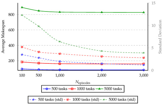
Figure 7. Effect of $N_{\mathrm{episodes}}$ on makespan (left axis) and standard deviation (right axis).

As $N_{\mathrm{episodes}}$ increases from 100 to 3000, all three workload sizes exhibit a clear reduction in makespan, especially within the range of 100 to 1000 episodes. For example, in the 500-nodes workload, the average makespan drops from 93.2 to 81.7 as the number of episodes increases from 100 to 1000. However, beyond 1000 episodes, the improvement becomes marginal, e.g., only a 1.4 reduction between 1000 and 3000, suggesting a diminishing return from further training. Meanwhile, the standard deviation decreases steadily across all workload sizes, indicating that more training episodes lead to more stable scheduling decisions. For instance, the standard deviation for the 5000-nodes workload decreases from 12.3 at 100 episodes to 3.9 at 3000 episodes. This confirms that increased training helps the DDQN component converge to more consistent policies.

In summary, increasing $N_{\mathrm{episodes}}$ improves both scheduling quality and stability up to a certain point, beyond which additional training yields little benefit. A value around 1000 to 2000 appears to offer a good trade-off between performance and training cost.

5.3.2. Impact of Discount Factor $\gamma$

To evaluate the impact of the discount factor $\gamma$ on the learning performance of the DDQN-based scheduling strategy within the WORL-RTGS framework, we perform a parameter sensitivity analysis by varying $\gamma$ while keeping all other hyperparameters fixed at their default values. The discount factor $\gamma \in (0,1)$ plays a pivotal role in balancing the importance of immediate versus future rewards. A smaller $\gamma$ places greater emphasis on short-term gains, whereas a larger value encourages long-term planning. In the context of GPU task scheduling, this trade-off directly influences how the algorithm prioritizes near-term scheduling efficiency versus delayed but globally optimal task placements.

As shown in Table 6, we consider five representative values of $\gamma$: 0.90, 0.93, 0.95, 0.97, 0.99, covering a wide range from myopic to far-sighted decision-making. Each configuration is evaluated using three benchmark DAG workloads with 500, 1000, and 5000 task nodes, respectively, drawn from the Alibaba Cluster Trace v2018, following the same experimental setup described in Section 5.3.1. Based on prior analysis of training episode sensitivity, we fix the number of training episodes at $N_{\mathrm{episodes}}=1000$ for all tests.

By examining how different values of $\gamma$ affect the learning stability and final cumulative reward, this experiment aims to reveal whether the scheduling policy benefits more from short-term optimization or long-term reward accumulation. The results help identify the most effective setting of $\gamma$ that ensures stable convergence and high-quality scheduling performance across diverse GPU workloads. Each test is repeated ten times to reduce the impact of randomness, and average results are reported.

To investigate the influence of the discount factor $\gamma$ on the learning dynamics and final scheduling performance of the DDQN-based strategy in WORL-RTGS, we perform a parameter sensitivity analysis across five representative values: $\gamma \in \{0.90,0.93,0.95,0.97,0.99\}$. Unlike traditional Reinforcement Learning setups that analyze convergence based on the number of training episodes alone, our setting involves a total of 9 million episodes, across three benchmark tasks, each involving 300 iterations × 10 whales × 1000 episodes. This renders the conventional notion of episode-based convergence unsuitable. To address this, we redefine the convergence speed metric. Specifically, we partition the entire training process into 9000 stages, each representing 1000 training episodes. At the end of each stage, training is paused, and the current DDQN policy is used in inference mode to schedule a test DAG with 500 task nodes. The Cumulative Reward and Stability (Std.) are recorded. This enables us to observe how the policy evolves and whether its scheduling quality improves as training progresses.

Figure 8 illustrates the cumulative reward progression for each $\gamma$ value across all stages. The results reveal that $\gamma =0.90$ exhibits faster early-stage improvement, but suffers from larger fluctuations and a lower overall performance ceiling. $\gamma =0.93$ balances stability and reward more effectively, showing smoother progression with improved final outcomes. $\gamma =0.95$ and $\gamma =0.97$ both demonstrate strong long-term optimization behaviors. In particular, $\gamma =0.97$ achieves the highest final cumulative reward 1401.8 with relatively low variance 64.9, indicating excellent convergence and generalization. $\gamma =0.99$, while conceptually emphasizing long-term reward, shows signs of slower adaptation and mild instability in early and middle stages, although its final performance remains competitive.

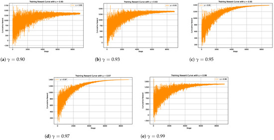
Figure 8. Parameter sensitivity analysis for different values of $\gamma$.

Table 8 further confirms these observations by summarizing the final reward and corresponding standard deviation across three test tasks: 500, 1000, and 5000 task nodes. The performance trend shows that a moderate-to-high discount factor (0.95–0.97) leads to the best overall trade-off between convergence speed, reward maximization, and stability. Taken together, these results suggest that $\gamma =0.97$ is the most effective setting under our workload characteristics, as it promotes both high reward accumulation and robust learning convergence throughout the prolonged training process. Therefore, in practical deployments of WORL-RTGS on large-scale GPU clusters, setting $\gamma$ within the range of 0.95–0.97 is recommended to ensure optimal scheduling quality and learning robustness.

Table 8. Final reward and stability (Std.) under different $\gamma$ values.

Task Size	$\mathit{\gamma }=0.90$		$\mathit{\gamma }=0.93$		$\mathit{\gamma }=0.95$		$\mathit{\gamma }=0.97$		$\mathit{\gamma }=0.99$
	Reward	Std.	Reward	Std.	Reward	Std.	Reward	Std.	Reward	Std.
500	1325.7	92.4	1358.9	75.2	1392.7	62.3	1401.8	64.9	1387.4	78.6
1000	2590.3	185.1	2684.1	142.5	2794.5	118.2	2831.0	126.1	2762.6	141.3
5000	12,845.6	548.2	13,242.8	504.6	13,872.4	465.8	14,034.7	478.3	13,759.5	512.7

5.3.3. Impact of Parameter b

For the subsequent experiments, we configure $N_{\mathrm{episodes}}$ to 1000 and $\gamma$ to 0.97, as determined by the evaluations in Section 5.3.1 and Section 5.3.2, while maintaining all other hyperparameters at their default settings. To examine the impact of parameter b in WORL-RTGS, we devise a series of controlled tests using three representative workloads, consistent with Section 5.3.1: a small job with 500 task nodes, a medium job with 1000 task nodes, and a large job with 5000 task nodes. This categorization enables us to assess the stability of parameter b across varying workload magnitudes.

For each chosen job, we run WORL-RTGS with different configurations of parameter b, varying from 0.5 to 2.0 in steps of 0.5, resulting in four values: $b\in \{0.5,1.0,1.5,2.0\}$. For every b value and job size, we conduct 30 trials of the algorithm, logging the makespan after each trial. Using this data, we create a box plot to visualize the makespan distribution across small, medium, and large jobs for each b value. In the plot, the x-axis indicates the b value, while the y-axis shows the makespan. To verify the statistical significance of performance disparities, we utilize non-parametric statistical methods: the Friedman test [48], succeeded by the Nemenyi post hoc test [49], applied to the makespan outcomes across various b values. The Friedman test’s lack of reliance on normal distribution assumptions renders it well suited for these scheduling experiments, allowing us to assess whether performance differences are statistically significant.

Figure 9 displays boxplots illustrating makespan distributions for three job sizes under different b values. The parameter b notably influences the algorithm’s effectiveness. In particular, when b falls within $[1.0,1.5]$, the algorithm consistently delivers improved performance, with shorter and more consistent job completion times across all job scales. Conversely, at extreme values like $b=0.5$ or $b\ge 2.0$, completion times show greater variability and often rise significantly, suggesting diminished scheduling efficiency and stability.

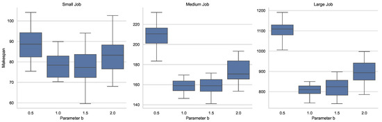
Figure 9. Completion time for small, medium, and large jobs across varying b values.

To evaluate the impact of the priority parameter b on scheduling efficiency, we conducted Friedman and Nemenyi post hoc tests on the makespan results under the four distinct b settings $[0.5,1.0,1.5,2.0]$, across three job sizes: small, medium, and large. The Friedman test results in Table 9 indicate statistically significant differences in makespan among different b values for all job sizes $p<0.01$. This validates that the choice of b has a non-negligible effect on the scheduling outcome.

Table 9. Friedman test results for different job sizes.

Job Size	Friedman Statistic	p-Value
Small	19.8400	0.0002
Medium	73.2400	0.0000
Large	71.5600	0.0000

Subsequent Nemenyi post hoc comparisons reveal several key insights. In the small job tests Table 10, settings $b=1.0$ and $b=1.5$ significantly outperform $b=0.5$, and there is no significant difference between them, suggesting these values are more appropriate for lightweight tasks. In the medium job tests Table 11, nearly all pairs differ significantly except between $b=1.0$ and $b=1.5$, indicating these two settings provide optimal makespan while $b=0.5$ consistently underperforms. In the large job tests Table 12, $b=0.5$ yields the worst performance. Both $b=1.0$ and $b=1.5$ are statistically better, while $b=2.0$ may introduce overhead or less balanced scheduling. In conclusion, while smaller b values lead to poorer performance, the values $b=1.0$ and $b=1.5$ consistently demonstrate statistically superior makespan outcomes across job types, making them favorable default choices in the WORL-RTGS scheduling algorithm.

Table 10. Nemenyi post hoc test p-values for small jobs.

	0.5	1.0	1.5	2.0
0.5	1.000	0.0018	0.0004	0.1879
1.0	0.0018	1.000	0.9783	0.3786
1.5	0.0004	0.9783	1.000	0.1879
2.0	0.1879	0.3786	0.1879	1.000

Table 11. Nemenyi post hoc test p-values for medium jobs.

	0.5	1.0	1.5	2.0
0.5	1.000	$3.12\times {10}^{-11}$	$1.78\times {10}^{-13}$	0.0026
1.0	$3.12\times {10}^{-11}$	1.000	0.8971	0.0038
1.5	$1.78\times {10}^{-13}$	0.8971	1.000	0.0002
2.0	0.0026	0.0038	0.0002	1.000

Table 12. Nemenyi post hoc test p-values for large jobs.

	0.5	1.0	1.5	2.0
0.5	1.000	$3.71\times {10}^{-14}$	$4.82\times {10}^{-10}$	0.0012
1.0	$3.71\times {10}^{-14}$	1.000	0.5629	0.0002
1.5	$4.82\times {10}^{-10}$	0.5629	1.000	0.0263
2.0	0.0012	0.0002	0.0263	1.000

5.3.4. Impact of Max Iterations

The parameters $N_{episodes}$, $\gamma$, and b are determined based on prior experiments. For subsequent tests, we configure $N_{episodes}$ to 1000, $\gamma$ to 0.97, and b to 1.0 to simplify the spiral update equation. To capture both short- and long-duration workloads, we select tasks with approximately 100–1000 nodes for short jobs and 1000–10,000 nodes for long jobs. To establish the maximum iteration count, we perform two experiment groups. The first group analyzes the makespans of jobs from the Alibaba Cluster Trace across iterations during the cluster’s busy phase. The second set of experiments assesses the total completion times of jobs during the cluster’s idle state. The findings are illustrated in Figure 10, with Figure 10a presenting results for the busy state and Figure 10b displaying outcomes for the idle state. It is observed that makespans reach stability after approximately 200 iterations in Figure 10a and 300 iterations in Figure 10b, suggesting a slower convergence rate during idle periods. Consequently, we set the iteration limit to 300 for subsequent experiments.

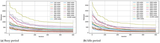
Figure 10. Makespan across iterations during busy and idle periods.

5.4. Ablation Study: Contribution of Hybrid Design

To directly evaluate the effectiveness of WORL-RTGS in overcoming the limitations of standalone Reinforcement Learning and traditional heuristic optimization WOA, we conduct an ablation study using real-world workloads. Job traces are sampled from the Alibaba Cluster Trace dataset, which reflects large-scale production workloads with diverse job sizes, resource demands, and execution patterns. We randomly select representative jobs covering small, medium, and large computational scales to maintain workload heterogeneity.

We compare the following variants to assess the contribution of each component:

• WORL-RTGS (full): Hybrid WOA-guided RL.
• WORL-RTGS w/o WOA: Pure DDQN with the same state-action space as the RL component in WORL-RTGS. The $\mathrm{hope}\left(l_i\right)$ value is set to the mean task load.
• WORL-RTGS w/o RL: Pure WOA with a fixed iteration budget. WOA is used as a standalone population-based optimizer to search the task-to-GPU mapping space, using the same makespan objective as the hybrid approach.

Table 13, Table 14 and Table 15 show that WORL-RTGS (full) consistently achieves the lowest mean makespan and highest scheduling stability across all tested job scales. Removing either the WOA or RL component leads to significant performance degradation, which becomes more pronounced as the job size increases.

Table 13. Ablation study on real workload with 300 nodes.

Algorithm	Mean Makespan (s)	Relative Increase	Std. Dev.	Relative Increase (Std. Dev.)
WORL-RTGS (full)	137.7	-	5.2	-
w/o WOA (pure DDQN)	315.4	+129.1%	12.8	+146.2%
w/o RL (pure WOA)	593.7	+331.2%	24.6	+373.1%

Table 14. Ablation study on real workload with 1000 nodes.

Algorithm	Mean Makespan (s)	Relative Increase	Std. Dev.	Relative Increase (Std. Dev.)
WORL-RTGS (full)	395.5	-	11.3	-
w/o WOA (pure DDQN)	876.2	+121.5%	26.7	+136.3%
w/o RL (pure WOA)	1638.4	+314.2%	63.8	+464.6%

Table 15. Ablation study on real workload with 5000 nodes.

Algorithm	Mean Makespan (s)	Relative Increase	Std. Dev.	Relative Increase (Std. Dev.)
WORL-RTGS (full)	287.9	-	9.1	-
w/o WOA (pure DDQN)	682.4	+137.0%	23.5	+158.2%
w/o RL (pure WOA)	1423.6	+394.3%	79.1	+769.2%

Specifically, under the 300-node workload, pure DDQN (w/o WOA) increases the mean makespan by 129.1%, while pure WOA (w/o RL) leads to an increase of 331.2%. Similar trends occur for larger jobs: the 1000-node case shows 121.5% (DDQN) and 314.2% (WOA) increases; the 5000-node case exhibits 137.0% and 394.3% increases, respectively. These results highlight the critical synergy between WOA’s global search and RL’s adaptive decision-making for scalability and convergence efficiency.

In terms of stability, WORL-RTGS has the lowest standard deviation in makespan. Pure DDQN shows 1.3–1.6× higher variability, while pure WOA fluctuates even more, up to 7.7× higher at 5000 nodes. This demonstrates that the hybrid design not only accelerates convergence but also ensures robust performance under dynamic workload variations.

Overall, the ablation study confirms that the WOA-guided RL architecture effectively integrates heuristic global exploration with data-driven policy optimization. Removing WOA leads to poor exploration, increasing makespan by up to 137%, whereas removing RL limits learned generalization, increasing makespan by up to 394%. Meanwhile, the hybrid design accelerates convergence (3.2× faster than pure DDQN), demonstrating robust and scalable performance in real-world cluster environments.

5.5. Comparison of Scheduling Algorithms on Real Workloads

Figure 11 presents a comparison of makespans for six scheduling algorithms: DRAS, mDRL, MAGRL, MIGMPS, RL-Hybrid, and WORL-RTGS. It highlights their performance in scheduling DAG-structured jobs during both high-load and low-load cluster periods. The horizontal axis represents the number of tasks, ranging from 100 to 1000 for short-running jobs and from 1000 to 10,000 for long-running jobs, all of which are extracted from the Alibaba dataset. The vertical axis represents the job makespan. Note that a lower job makespan indicates a better performance of the scheduler.

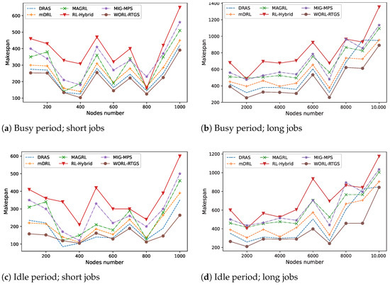
Figure 11. Experiments conducted on DAG-structured workloads.

Across all settings, WORL-RTGS consistently outperforms all other algorithms, achieving the lowest job makespan in both idle and busy environments, regardless of job size, as shown in Figure 11. This confirms the robustness and efficiency of the WORL-RTGS algorithm in optimizing task scheduling under diverse system loads. In contrast, RL-Hybrid consistently shows the worst performance, with significantly higher makespan values and larger fluctuations, especially in large job scenarios. This suggests that RL-Hybrid lacks sufficient generalization and adaptability when handling complex DAG dependencies or under high resource contention.

In idle cluster environments, both small and large job sets reveal noticeable performance differences despite the abundance of resources. WORL-RTGS consistently achieves the lowest makespan across all task sizes, demonstrating superior data locality and scheduling efficiency. DRAS and mDRL follow closely, although mDRL exhibits more variability with occasional spikes (e.g., 265 s at 900 tasks). MAGRL and MIGMPS show moderate performance but suffer from instability, indicated by intermittent makespan surges. RL-Hybrid performs the worst, especially for large jobs where its makespan reaches up to 1175 s, highlighting its poor scalability and limited optimization capability.

In busy cluster scenarios, where resource contention is intense, the differences between algorithms become more pronounced. WORL-RTGS remains the most robust, maintaining relatively low makespan values even under pressure (e.g., 891 s at 10,000 tasks). DRAS and mDRL show moderate degradation but remain competitive. In contrast, MAGRL and MIGMPS struggle with increased volatility and frequent performance drops, particularly in large-job scenarios.

The Friedman test yields a p-value $<0.001$ for all conditions, indicating statistically significant performance differences among algorithms at $\alpha =0.05$. This confirms that at least one algorithm performs significantly differently from the others under each tested condition. As indicated by the Nemenyi post hoc analysis in Table 16, WORL-RTGS maintains the highest average ranking in all conditions, spanning from 1.00 to 2.61. The bar chart in Figure 12 illustrates the average ranks of six scheduling algorithms based on the Nemenyi test. This highlights its superior and stable scheduling performance for DAG-structured jobs, regardless of task size or resource availability. DRAS and mDRL also show relatively strong performance, typically ranking just behind WORL-RTGS. DRAS is particularly competitive in small-task scenarios, while mDRL maintains steady ranks around 2.5–3.0. These results suggest they are effective but slightly less robust under high-load or large-scale task conditions. In contrast, MAGRL and MIGMPS demonstrate moderate rankings and show signs of declining effectiveness as the task scale increases or under busy conditions. RL-Hybrid consistently ranks the worst, indicating poor scalability and adaptation in DAG-based scheduling. Overall, the ranking trends reflect that algorithms with stronger learning and optimization capabilities particularly WORL-RTGS are better equipped to handle the complexity of DAG task dependencies under varying system loads.

Table 16. Nemenyi test: average ranks for DAG Real task scheduling.

	DRAS	mDRL	MAGRL	MIGMPS	RL-Hybrid	WORL-RTGS
Small Tasks (High Load)	2.11	3.11	3.78	4.67	6.00	1.33
Large Tasks (High Load)	2.10	3.00	4.20	4.90	5.90	1.00
Small Tasks (Low Load)	1.61	2.56	3.78	4.56	6.00	2.61
Large Tasks (Low Load)	2.10	3.00	4.25	4.65	5.70	1.00

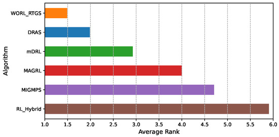
Figure 12. Critical difference diagram.

5.6. Comparison of Scheduling Algorithms on Synthetic Workloads

To evaluate performance under controlled conditions, we conduct experiments with synthetically generated workloads. Our evaluation examines system performance under both high-load and low-load server conditions. In the busy state, each GPU’s resource utilization rate is randomly sampled from the range $[50,80]$, while in the idle state, it is drawn from $[10,50]$, reflecting typical variations in system load. We construct 27 DAG-topology jobs using the Erdos–Rényi model [45], setting the average in-degree/out-degree to 100. The workload sizes are designed to cover a spectrum: small-scale jobs consist of 100 to 1000 nodes in steps of 100, medium-scale jobs range from 1200 to 3000 nodes in steps of 200, and large-scale jobs span 4000 to 10,000 nodes in steps of 1000. Job execution times are sampled from normal distributions $N(2,1^2)$ for small-scale, medium-scale, large-scale workloads. For each combination of system state (busy/idle) and job scale (small/medium/large), we conduct 100 independent repetitions to ensure statistical reliability and reduce the influence of randomness. This comprehensive design not only provides a diverse set of workload conditions but also enables a rigorous evaluation of algorithm performance across varying levels of resource contention, structural complexity, and workload intensity.

Figure 13 reports the performance comparison of six scheduling algorithms under synthetic workloads across both busy and idle environments, and for job scales ranging from small to large. For small workloads, WORL-RTGS consistently achieves the lowest completion times, with DRAS and mDRL slightly higher (3–7%). MAGRL, MIGMPS, and RL-Hybrid incur higher overhead, performing worse under busy conditions. In medium-scale workloads, the advantage of WORL-RTGS diminishes. DRAS and mDRL outperform it in several cases, while MAGRL and MIGMPS become competitive, especially in idle environments. For large workloads, learning-based schedulers show clear benefits. WORL-RTGS reduces completion time by over 10% compared to MIGMPS and RL-Hybrid in idle settings, demonstrating stronger scalability.

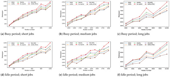
Figure 13. Experiments conducted on Synthetic DAG-structured workloads.

The Friedman tests for all synthetic workload scenarios yield $p<0.001$, confirming statistically significant performance differences at $\alpha =0.05$. The statistical analysis of algorithm performance on synthetic DAG-structured tasks, as presented in Table 17, Table 18 and Table 19, reveals significant differences across all tested conditions, with Friedman test ${\chi }^2$ statistics ranging from 34.80 to 46.10 and $p<0.001$ in all cases, confirming statistical significance at $\alpha =0.05$. The Nemenyi post hoc test further elucidates pairwise performance differences, with average ranks indicating that WORL-RTGS consistently outperforms others, achieving the lowest rank (1.00–1.14) across all conditions, followed closely by DRAS (2.00–2.20). Critical difference (CD) is 3.374 for small and medium tasks (n = 10), and 4.033 for large tasks (n = 7). Pairwise differences exceeding CD are significant (p < 0.05). For large tasks under low load (Table 19), WORL-RTGS (1.00) and DRAS (2.00) maintain superior performance, while mDRL and MAGRL share an identical rank of 3.86, suggesting comparable performance. MIGMPS (4.43) and RL-Hybrid (5.86) rank lower, with RL-Hybrid consistently performing the worst. With a Critical difference (CD) of 4.033 for large tasks (n = 7), the rank difference between WORL-RTGS and RL-Hybrid (4.86) exceeds the CD, indicating a statistically significant performance advantage for WORL-RTGS over RL-Hybrid ($p<0.05$). However, differences between other pairs, such as WORL-RTGS and DRAS (1.00) or mDRL and MAGRL (0.00), do not exceed the CD, suggesting no significant differences in those cases. These results highlight WORL-RTGS as the most effective algorithm, particularly under varying load conditions and task scales, while RL-Hybrid consistently underperforms.

Table 17. Statistical analysis of algorithm performance on DAG-structured synthetic tasks across various conditions.

Condition	${\mathit{\chi }}^2$ Statistic
Small Tasks (High Load)	38.50
Medium Tasks (High Load)	39.20
Large Tasks (High Load)	46.10
Small Tasks (Low Load)	34.80
Medium Tasks (Low Load)	35.60
Large Tasks (Low Load)	44.50

Table 18. Nemenyi test: average ranks under different task sizes and load conditions.

	WORL-RTGS	DRAS	mDRL	MAGRL	MIGMPS	RL-Hybrid
Small Tasks (High Load)	1.00	2.00	3.10	4.20	4.70	6.00
Medium Tasks (High Load)	1.10	2.00	2.90	4.40	4.60	6.00
Large Tasks (High Load)	1.14	2.14	2.86	4.43	4.43	6.00
Small Tasks (Low Load)	1.00	2.00	3.20	4.00	4.90	5.90
Medium Tasks (Low Load)	1.00	2.20	3.00	4.10	4.90	5.80
Large Tasks (Low Load)	1.00	2.00	3.86	3.86	4.43	5.86

Table 19. Nemenyi test: overall average ranks across all task configurations.

Algorithm	Average Rank
WORL-RTGS	1.04
DRAS	2.06
mDRL	3.15
MAGRL	4.17
MIGMPS	4.66
RL-Hybrid	5.93

6. Conclusions and Future Work

In today’s computing landscape, orchestrating Directed Acyclic Graph (DAG)-structured machine learning tasks stands as a cornerstone for numerous cutting-edge applications. These tasks, which permeate Deep Neural Network training workflows, data analytics platforms such as Apache Spark and TensorFlow, and extensive model adaptation efforts, leverage DAG topologies to navigate complex task interdependencies and ensure orderly execution. Achieving optimal task prioritization and resource distribution is paramount for maximizing efficiency and throughput, particularly in heterogeneous or capacity-constrained infrastructures where parallelism and scalability are often challenged by varying hardware capabilities and dynamic demands.

In this work, we investigated a task scheduling problem for DAG-structured workloads on a parallel computing platform with virtual or physical servers. This problem is proved to be NP-complete. We revealed an important positive correlation between $\mathit{SPD}$ and $\mathit{FTG}$, and by leveraging this finding, we proposed a novel algorithm WORL-RTGS based on the WOA algorithm and DDQN framework. In WORL-RTGS, we derived a function to generate the humpback’s next step, and designed a DDQN algorithm to satisfy each server’s load demand. Comprehensive evaluations using both real-world workload traces and artificially generated data demonstrate that WORL-RTGS outperforms five leading baseline algorithms.

We aim to refine the $\mathit{SPD}$ function to create novel scheduling strategies that precisely guide the trajectory of each iteration. Additionally, a future goal is to establish a robust decision framework to identify the optimal workload types for WORL-RTGS, enhancing its effectiveness and service quality in large-scale data processing systems.

References

- Garefalakis, P.; Karanasos, K.; Pietzuch, P.; Suresh, A.; Rao, S. Medea: Scheduling of long running applications in shared production clusters. In Proceedings of the Thirteenth EuroSys Conference, Porto, Portugal, 23–26 April 2018; pp. 1–13. [Google Scholar]
- Sun, P.; Guo, Z.; Wang, J.; Li, J.; Lan, J.; Hu, Y. Deepweave: Accelerating job completion time with deep reinforcement learning-based coflow scheduling. In Proceedings of the Twenty-Ninth International Conference on International Joint Conferences on Artificial Intelligence (IJCAI 29), Yokohama, Japan, 11–17 July 2021; pp. 3314–3320. [Google Scholar]
- Google, C.N.C.F. What Is Kubernetes. Website, 2017. Available online: https://kubernetes.io/docs/concepts/overview/what-is-kubernetes/ (accessed on 6 November 2025).
- Vavilapalli, V.K.; Murthy, A.C.; Douglas, C.; Agarwal, S.; Konar, M.; Evans, R.; Graves, T.; Lowe, J.; Shah, H.; Seth, S.; et al. Apache hadoop yarn: Yet another resource negotiator. In Proceedings of the 4th Annual Symposium on Cloud Computing, Santa Clara, CA, USA, 1–3 October 2013; pp. 1–16. [Google Scholar]
- Hindman, B.; Konwinski, A.; Zaharia, M.; Ghodsi, A.; Joseph, A.D.; Katz, R.; Shenker, S.; Stoica, I. Mesos: A Platform for Fine-Grained Resource Sharing in the Data Center. In Proceedings of the 8th USENIX Symposium on Networked Systems Design and Implementation (NSDI 11), Boston, MA, USA, 30 March–1 April 2011. [Google Scholar]
- Mao, H.; Schwarzkopf, M.; Venkatakrishnan, S.B.; Meng, Z.; Alizadeh, M. Learning scheduling algorithms for data processing clusters. In Proceedings of the ACM Special Interest Group on Data Communication (SIGCOMM 2019), Beijing, China, 19–23 August 2019; pp. 270–288. [Google Scholar]
- Mirjalili, S.; Lewis, A. The whale optimization algorithm. Adv. Eng. Softw. 2016, 95, 51–67. [Google Scholar] [CrossRef]
- Du, N.; Ji, Y.; Wu, C.; Hou, A.; Nie, W. Scheduling DAG-structured workloads based on whale optimization algorithm: N. Du et al. J. Supercomput. 2025, 81, 911. [Google Scholar] [CrossRef]
- Pan, J.; Wei, Y.; Meng, L.; Meng, X. A dual scheduling framework for task and resource allocation in clouds using deep reinforcement learning. J. King Saud Univ. Comput. Inf. Sci. 2025, 37, 81. [Google Scholar] [CrossRef]
- Gao, Y.; Yi, H.; Chen, H.; Fang, X.; Zhao, S. A structure-aware DAG scheduling and allocation on heterogeneous multicore systems. In Proceedings of the 2024 IEEE 14th International Symposium on Industrial Embedded Systems (SIES), Chengdu, China, 23–25 October 2024; IEEE: Piscataway, NJ, USA, 2024; pp. 26–33. [Google Scholar]
- Gao, W.; Ye, Z.; Sun, P.; Wen, Y.; Zhang, T. Chronus: A novel deadline-aware scheduler for deep learning training jobs. In Proceedings of the ACM Symposium on Cloud Computing, Seattle, WA, USA, 1–4 November 2021; pp. 609–623. [Google Scholar]
- Hu, Q.; Sun, P.; Yan, S.; Wen, Y.; Zhang, T. Characterization and prediction of deep learning workloads in large-scale gpu datacenters. In Proceedings of the International Conference for High Performance Computing, Networking, Storage and Analysis, St. Louis, MO, USA, 14–19 November 2021; pp. 1–15. [Google Scholar]
- Cheng, L.; Kalapgar, A.; Jain, A.; Wang, Y.; Qin, Y.; Li, Y.; Liu, C. Cost-aware real-time job scheduling for hybrid cloud using deep reinforcement learning. Neural Comput. Appl. 2022, 34, 18579–18593. [Google Scholar] [CrossRef]
- Chen, P.; Chen, H.; Liu, W.; Long, L.; Chang, W.; Guan, N. Dag-order: An order-based dynamic dag scheduling for real-time networks-on-chip. ACM Trans. Archit. Code Optim. 2023, 21, 1–24. [Google Scholar] [CrossRef]
- Zhao, S.; Dai, X.; Bate, I. DAG scheduling and analysis on multi-core systems by modelling parallelism and dependency. IEEE Trans. Parallel Distrib. Syst. 2022, 33, 4019–4038. [Google Scholar] [CrossRef]
- Fan, S.; Rong, Y.; Meng, C.; Cao, Z.; Wang, S.; Zheng, Z.; Wu, C.; Long, G.; Yang, J.; Xia, L.; et al. DAPPLE: A pipelined data parallel approach for training large models. In Proceedings of the 26th ACM SIGPLAN Symposium on Principles and Practice of Parallel Programming, Virtually, 27 February–3 March 2021; pp. 431–445. [Google Scholar]
- Liang, S.; Yang, Z.; Jin, F.; Chen, Y. Data centers job scheduling with deep reinforcement learning. In Proceedings of the Pacific-Asia Conference on Knowledge Discovery and Data Mining, Singapore, 11–14 May 2020; Springer: Berlin/Heidelberg, Germany, 2020; pp. 906–917. [Google Scholar]
- Zheng, T.; Wan, J.; Zhang, J.; Jiang, C. Deep reinforcement learning-based workload scheduling for edge computing. J. Cloud Comput. 2022, 11, 3. [Google Scholar] [CrossRef]
- Peng, Y.; Bao, Y.; Chen, Y.; Wu, C.; Meng, C.; Lin, W. DL2: A deep learning-driven scheduler for deep learning clusters. IEEE Trans. Parallel Distrib. Syst. 2021, 32, 1947–1960. [Google Scholar] [CrossRef]
- Ye, Z.; Gao, W.; Hu, Q.; Sun, P.; Wang, X.; Luo, Y.; Zhang, T.; Wen, Y. Deep learning workload scheduling in gpu datacenters: A survey. ACM Comput. Surv. 2024, 56, 1–38. [Google Scholar] [CrossRef]
- Li, Z.; Zhuang, S.; Guo, S.; Zhuo, D.; Zhang, H.; Song, D.; Stoica, I. Terapipe: Token-level pipeline parallelism for training large-scale language models. In Proceedings of the International Conference on Machine Learning, PMLR, Virtual Event, 18–24 July 2021; pp. 6543–6552. [Google Scholar]
- Zhang, J.; Niu, G.; Dai, Q.; Li, H.; Wu, Z.; Dong, F.; Wu, Z. PipePar: Enabling fast DNN pipeline parallel training in heterogeneous GPU clusters. Neurocomputing 2023, 555, 126661. [Google Scholar] [CrossRef]
- Mondal, S.S.; Sheoran, N.; Mitra, S. Scheduling of time-varying workloads using reinforcement learning. In Proceedings of the AAAI Conference on Artificial Intelligence, Virtual Event, 19–21 May 2021; Volume 35, pp. 9000–9008. [Google Scholar]
- Islam, M.T.; Karunasekera, S.; Buyya, R. Performance and cost-efficient spark job scheduling based on deep reinforcement learning in cloud computing environments. IEEE Trans. Parallel Distrib. Syst. 2021, 33, 1695–1710. [Google Scholar] [CrossRef]
- Hegde, S.N.; Srinivas, D.; Rajan, M.; Rani, S.; Kataria, A.; Min, H. Multi-objective and multi constrained task scheduling framework for computational grids. Sci. Rep. 2024, 14, 6521. [Google Scholar] [CrossRef] [PubMed]
- Sudhakar, R.V.; Dastagiraiah, C.; Pattem, S.; Bhukya, S. Multi-Objective Reinforcement Learning Based Algorithm for Dynamic Workflow Scheduling in Cloud Computing. Indones. J. Electr. Eng. Inform. (IJEEI) 2024, 12, 640–649. [Google Scholar] [CrossRef]
- Gu, R.; Chen, Y.; Liu, S.; Dai, H.; Chen, G.; Zhang, K.; Che, Y.; Huang, Y. Liquid: Intelligent resource estimation and network-efficient scheduling for deep learning jobs on distributed GPU clusters. IEEE Trans. Parallel Distrib. Syst. 2021, 33, 2808–2820. [Google Scholar] [CrossRef]
- Yeung, G.; Borowiec, D.; Yang, R.; Friday, A.; Harper, R.; Garraghan, P. Horus: Interference-aware and prediction-based scheduling in deep learning systems. IEEE Trans. Parallel Distrib. Syst. 2021, 33, 88–100. [Google Scholar] [CrossRef]
- Fan, Y.; Li, B.; Favorite, D.; Singh, N.; Childers, T.; Rich, P.; Allcock, W.; Papka, M.E.; Lan, Z. Dras: Deep reinforcement learning for cluster scheduling in high performance computing. IEEE Trans. Parallel Distrib. Syst. 2022, 33, 4903–4917. [Google Scholar] [CrossRef]
- Saroliya, U.; Arima, E.; Liu, D.; Schulz, M. Hierarchical resource partitioning on modern gpus: A reinforcement learning approach. In Proceedings of the 2023 IEEE International Conference on Cluster Computing (CLUSTER), Santa Fe, NM, USA, 31 October–3 November 2023; IEEE: Piscataway, NJ, USA, 2023; pp. 185–196. [Google Scholar]
- Zhao, X.; Wu, C. Large-scale machine learning cluster scheduling via multi-agent graph reinforcement learning. IEEE Trans. Netw. Serv. Manag. 2021, 19, 4962–4974. [Google Scholar] [CrossRef]
- Narantuya, J.; Shin, J.S.; Park, S.; Kim, J. Multi-Agent Deep Reinforcement Learning-Based Resource Allocation in HPC/AI Converged Cluster. Comput. Mater. Contin. 2022, 72, 4375–4395. [Google Scholar] [CrossRef]
- Ryu, J.; Eo, J. Network contention-aware cluster scheduling with reinforcement learning. In Proceedings of the 2023 IEEE 29th International Conference on Parallel and Distributed Systems (ICPADS), Danzhou, China, 17–21 December 2023; IEEE: Piscataway, NJ, USA, 2023; pp. 2742–2745. [Google Scholar]
- Zhang, L.; Shi, S.; Chu, X.; Wang, W.; Li, B.; Liu, C. Dear: Accelerating distributed deep learning with fine-grained all-reduce pipelining. In Proceedings of the 2023 IEEE 43rd International Conference on Distributed Computing Systems (ICDCS), Hong Kong, China, 18–21 July 2023; IEEE: Piscataway, NJ, USA, 2023; pp. 142–153. [Google Scholar]
- Brown, T.; Mann, B.; Ryder, N.; Subbiah, M.; Kaplan, J.D.; Dhariwal, P.; Neelakantan, A.; Shyam, P.; Sastry, G.; Askell, A.; et al. Language models are few-shot learners. Adv. Neural Inf. Process. Syst. 2020, 33, 1877–1901. [Google Scholar]
- Achiam, J.; Adler, S.; Agarwal, S.; Ahmad, L.; Akkaya, I.; Aleman, F.L.; Almeida, D.; Altenschmidt, J.; Altman, S.; Anadkat, S.; et al. Gpt-4 technical report. arXiv 2023, arXiv:2303.08774. [Google Scholar] [CrossRef]
- Goldberg, D. What every computer scientist should know about floating-point arithmetic. ACM Comput. Surv. (CSUR) 1991, 23, 5–48. [Google Scholar] [CrossRef]
- Choquette, J.; Gandhi, W.; Giroux, O.; Stam, N.; Krashinsky, R. Nvidia a100 tensor core gpu: Performance and innovation. IEEE Micro 2021, 41, 29–35. [Google Scholar] [CrossRef]
- Karp, R.M. Reducibility among combinatorial problems. In Complexity of Computer Computations; Springer: New York, NY, USA, 1972; pp. 85–103. [Google Scholar]
- Cormen, T.H.; Leiserson, C.E.; Rivest, R.L.; Stein, C. Topological sort. In Introduction to Algorithms, 2nd ed.; MIT Press: Cambridge, MA, USA, 2001; Chapter 22.4; pp. 549–552. [Google Scholar]
- Cormen, T.H.; Leiserson, C.E.; Rivest, R.L.; Stein, C. Single-source shortest paths in directed acyclic graphs. In Introduction to Algorithms, 2nd ed.; MIT Press: Cambridge, MA, USA, 2001; Chapter 24.2; pp. 592–595. [Google Scholar]
- Galton, F. Regression towards mediocrity in hereditary stature. J. Anthropol. Inst. Great Br. Irel. 1886, 15, 246–263. [Google Scholar] [CrossRef]
- Mapetu, J.P.B.; Kong, L.; Chen, Z. A dynamic VM consolidation approach based on load balancing using Pearson correlation in cloud computing. J. Supercomput. 2021, 77, 5840–5881. [Google Scholar] [CrossRef]
- Chiang, M.L.; Hsieh, H.C.; Cheng, Y.H.; Lin, W.L.; Zeng, B.H. Improvement of tasks scheduling algorithm based on load balancing candidate method under cloud computing environment. Expert Syst. Appl. 2023, 212, 118714. [Google Scholar] [CrossRef]
- ERDdS, P.; R&wi, A. On random graphs I. Publ. Math. Debr. 1959, 6, 18. [Google Scholar] [CrossRef]
- Goldbogen, J.A.; Friedlaender, A.S.; Calambokidis, J.; McKenna, M.F.; Simon, M.; Nowacek, D.P. Integrative approaches to the study of baleen whale diving behavior, feeding performance, and foraging ecology. BioScience 2013, 63, 90–100. [Google Scholar] [CrossRef]
- Watkins, W.A.; Schevill, W.E. Aerial observation of feeding behavior in four baleen whales: Eubalaena glacialis, Balaenoptera borealis, Megaptera novaeangliae, and Balaenoptera physalus. J. Mammal. 1979, 60, 155–163. [Google Scholar] [CrossRef]
- Friedman, M. The use of ranks to avoid the assumption of normality implicit in the analysis of variance. J. Am. Stat. Assoc. 1937, 32, 675–701. [Google Scholar] [CrossRef]
- Nemenyi, P.B. Distribution-Free Multiple Comparisons; Princeton University: Princeton, NJ, USA, 1963. [Google Scholar]
Disclaimer/Publisher’s Note: The statements, opinions and data contained in all publications are solely those of the individual author(s) and contributor(s) and not of MDPI and/or the editor(s). MDPI and/or the editor(s) disclaim responsibility for any injury to people or property resulting from any ideas, methods, instructions or products referred to in the content. |
© 2025 by the authors. Licensee MDPI, Basel, Switzerland. This article is an open access article distributed under the terms and conditions of the Creative Commons Attribution (CC BY) license (https://creativecommons.org/licenses/by/4.0/).