Assessment of Large-Eddy Simulations to Simulate a High-Speed Low-Pressure Turbine Cascade ^†

Abstract

The development of compact high-speed low-pressure turbines with high efficiencies requires the characterization of the secondary flow structures and the interaction of cavity purge and leakage flows with the mainstream. During the SPLEEN project funded by the European Union’s Horizon 2020, the von Karman Institute and Safran Aircraft Engines performed detailed measurements of low-pressure turbines in engine-realistic conditions (i.e., low Reynolds and high exit Mach numbers considering background turbulence, wakes, row interactions, and leakages). The SPLEEN project is thus a fundamental contribution to the progress of high-speed low-pressure turbines by delivering unique experimental databases, essential to characterize the time-resolved 3D turbine flow, and new critical knowledge to mature the design of 3D technological effects. Being able to simulate the flow and associated losses in such a configuration is both challenging and of paramount importance to help the understanding of the flow physics complementing experimental measurements. This paper focuses on the high-fidelity numerical simulation of one of the SPLEEN configuration consisting of a linear blade cascade. The objective is to provide a validated numerical setup in terms of computational domain, boundary conditions, mesh resolution and numerical scheme to reproduce the experimental results. By mean of wall-resolved large-eddy simulations, the design point characterized by an exit Mach number of 0.9 and an exit Reynolds number of 70,000 with a turbulence level of 2.4% is investigated for the baseline configuration without purge and without wake generator. The results show that the considered computational domain and the associated inlet total pressure profile play a critical role on the development of secondary flows. The isentropic Mach number distribution around the blade is shown to be robust to the mesh and numerical scheme. The development of the wake and secondary flow fields are drastically influenced by the mesh resolution and numerical scheme, impacting the resulting losses.

1. Introduction

This study, which is an extended version of the ETC2025-292 meeting paper published in the Proceedings of the 16th European Turbomachinery Conference [1], focuses on the examination of secondary flow effects in high-speed, low-pressure turbines (LPT), as detailed by the SPLEEN project (https://www.h2020-spleen.eu/). This European initiative aims to enhance the understanding and development of numerical tools for designing the next-generation of turbines by experimentally instrumenting a linear blade cascade under engine-realistic conditions. These advanced high-speed low-pressure turbines are crucial for the advancement of ultra high bypass ratio (UHBR) turbofans. A UHBR turbofan features a larger fan diameter than conventional ones, necessitating a lower fan rotation speed to minimize tip losses. Typically, this reduction in fan rotation speed is achieved through a gearbox connecting the fan rotor to the intermediate pressure compressor (IPC) [2]. Since the IPC and LPT are mechanically linked, the LPT can operate at a higher rate, optimizing the speeds of both the fan and the low-pressure turbine. This design strategy enhances overall cycle efficiency compared to current turbofans [3]. As engine efficiency continues to improve, the combustion chamber exit temperature rises, leading to hotter mainstream gas reaching the downstream turbines, which could potentially cause damage. To mitigate this risk, cooling films are introduced through small holes in the high-pressure turbine blades and walls, and purge flow is directed through cavities in the hub of axial turbines to prevent hot air from entering interstage gaps [4]. These purge flows are essential for engine operation and can constitute up to 20% of the main compressor flow used for cooling components [5]. Understanding the impact of purge flows on gas turbine efficiency is crucial, as increasing engine pressure ratios and bypass ratios exacerbate the penalties associated with cooling airflows [6]. Hence, a deeper understanding of secondary and leakage flows is necessary to optimize future high-speed LPTs. UHBR engine designs require LPTs to operate at transonic exit Mach numbers ($M_{out}>0.9$) and low Reynolds numbers [7]. Numerical simulation tools for turbomachinery flows are becoming increasingly sophisticated, yet simulating high-speed LPT conditions remains challenging due to issues such as shock development, boundary layer transition, and rotor–stator interactions. Current modeling approaches use unsteady Reynolds averaged Navier–Stokes (URANS) or large-eddy simulation (LES) [8,9,10,11] to capture unsteady phenomena. This unsteadiness is particularly important for studying purge flow effects. Denton [12] intuitively explains that purge flows contribute to mixing, which is closely related to entropy creation and losses in a turbomachine. Research by Gallier et al. [13] has shown that purge flows alter the formation of the horseshoe vortex. More recent studies [11,14] have demonstrated that secondary flows at the hub are influenced by purge flow, leading to increased friction and entropy production. Turbulence plays a critical role in turbomachinery simulations, affecting vortex behavior, boundary layer transition, and flow attachment around the blades [15]. Afshar et al. [16] recently conducted an isotropy turbulence analysis for a linear LPT cascade and found that LES accurately predicts turbulence transition and captures strongly anisotropic turbulent characteristics. Conversely, URANS struggles to capture these anisotropic phenomena, which impairs prediction accuracy, particularly in turbomachinery flows with frequent separation and boundary layer transition.

Different authors started to simulate the SPLEEN cascade configuration based on high-fidelity unsteady approaches. Boudin et al. [17], Hullin et al. [18] and Tene Hedje et al. [19,20] performed LES of a reduced span configuration to investigates the effect of the inlet turbulence an incoming wakes due to upstream moving cylinders, as well as the operating point on the flow structure at mid-span. These studies illustrate that LES well captures the flow development compared to experiments for the operating conditions investigated in terms of pressure distribution around the profile as well as losses in the wake region. Hullin et al. [18] and Perkins and Duchaine [21] simulated the full span of the linear cascade to investigate the effect of secondary flows in the hub region such as passage vortex and trailing shed vortex, as well as corner stall vortex. Both studies report very similar pressure loss patterns downstream of the blades compared to experiments. Additionally, Perkins and Duchaine [21] investigated the effect of the purge flow without incoming wakes, a configuration no treated experimentally. As expected, introducing the cavity and adding purge flow increased the losses in the blade passage.

The present work is a step forward in the validation of the numerical methodology based on the large-eddy simulation solver AVBP improving the results obtained by Perkins and Duchaine [21]. It was shown in this previous work that the yaw angle profile upstream of the blade was not well reproduced by the simulation and that the hub boundary layer was too thin compared to the experimental measurements. It is anticipated that these discrepancies results in angle and loss coefficient profiles downstream of the blade with almost good levels but the peak location shifted towards the hub compared to experimental results. To increase the reliability of the results before studying more complex cases including purge flow effect as well as incoming moving wake, this paper investigates the effect of the computational domain associated with inlet conditions, mesh resolution and numerical scheme accuracy.

The rest of this paper is organized as follows. First the SPLEEN configuration is introduced. The numerical solver used is then described along with the domain of investigation. The boundary condition, numerics, and meshes used are then detailed. Finally, the results section reports the sensitivity of the simulations to the mesh and numerical scheme.

2. SPLEEN Cascade Configuration

The SPLEEN linear cascade is described in details in a public database hosted on Zenodo [22]. The cascade is highly experimentally instrumented including particle image velocimetry (PIV) data [23], with additional characterization on the turbulence [24]. This cascade can also simulate the impacts of unsteady wakes between blade rows with moving bars as well as purge flows [25].

The cascade consists of 23 blades with a span of H = 165 mm. Other key dimensions are a blade chord, C, of $52.280$ mm, an axial chord, $C_{ax}$, of $47.614$ mm, and a pitch, g, of $32.950$ mm. The operating point retained for this study is described by an outlet Mach number, $M_{out}=0.90$ and by an outlet Reynolds number, $R{e}_{out}$ = 70,000. The freestream turbulence intensity was determined to be approximately $2.4\%$, generated by a grid just upstream of the test section. The cascade can simulate unsteady wakes with a spoked-wheel wake generator with 1 mm diameter cylindrical rods (yellow component in Figure 1). After this optional wake generator, a cavity used to inject purge/leakage flow into the test section with purge mass flow ratios ranging between 0 and $0.9\%$ of the mean main flow can be installed. Both the wake generators and the purge cavity are not included in the present study.

Experimental data are collected using four types of probes: static pressure taps (Ps taps in Figure 1), a pneumatic Cobra five-hole probe (C5HP), a pneumatic virtual four-hole cylindrical probe (PV4H), and a pneumatic L-shaped five-hole probe (L5HP). The static pressure taps at Plane 01 are used to characterize the inlet static pressure. The C5HP measures the total pressure as well as the pitch and yaw angle at Plane 02. The PV4H also measures the total pressure and pitch and yaw angle, but a fast-response version of this probe also exists to measure the unsteadiness of these conditions. Lastly, the L5HP is used to measure the outlet total pressure and pitch and yaw angle. Plane 02 (located half an axial chord upstream of the leading edge) is used to characterize the inlet flow field of total pressure and incidence on the blades. Plane 06 (located half an axial chord downstream of the trailing edge) is used to characterize the cascade losses and deviation.

3. Numerical Methodology

3.1. Numerical Solver

The Navier–Stokes equations are solved using CERFACS’ LES code, AVBP. This solver uses a cell-vertex approach on an unstructured multi-element grid. Two different convective schemes are compared in this work: the second-order in time and space Lax–Wendroff (LW) [26] scheme and the third-order in time and space TTGA4 [27] scheme. These schemes are explicit in time and a CFL number of 0.9 is used. The diffusive scheme is the finite element $2\mathrm{\Delta }$ scheme developed by O. Colin [28]. The subgrid-scale model used is the wall-adapting local eddy viscosity (WALE) [29], which is well suited for determining the eddy viscosity near walls in a wall-resolved context and is commonly used in LES of turbomachinery [11,21,30].

3.2. Computational Domain, Meshes, and Boundary Conditions

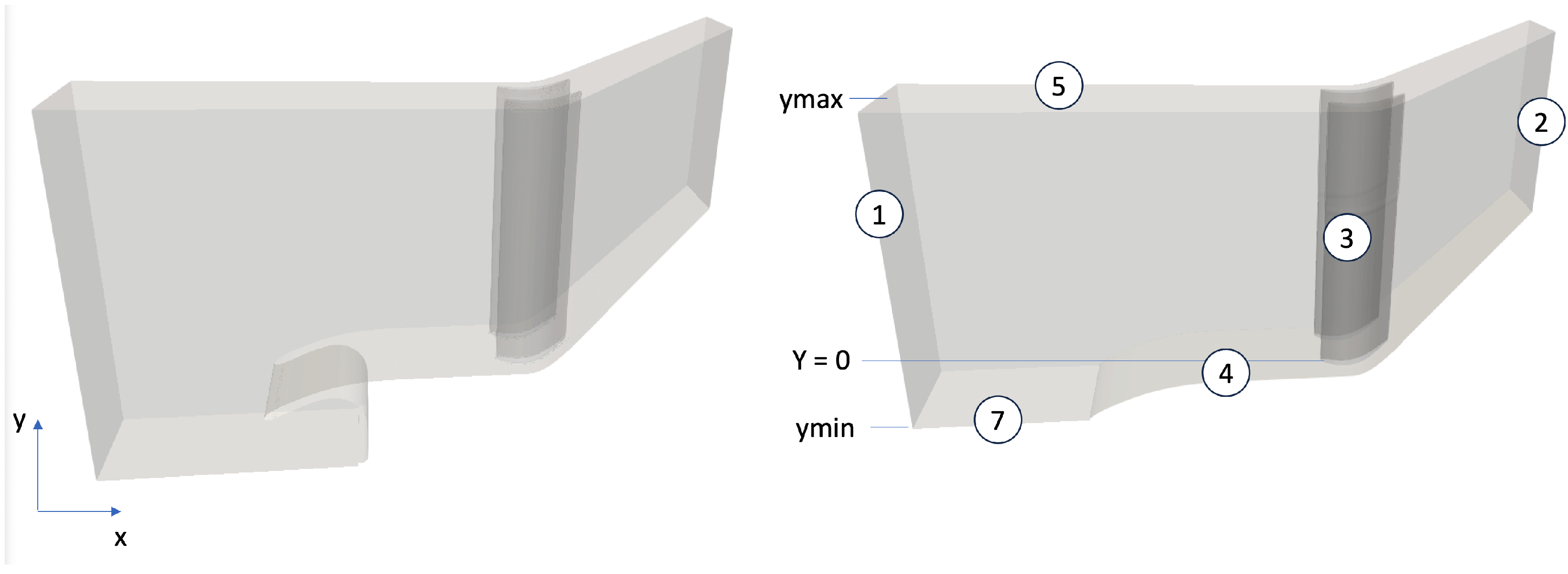
The computational domain comprises two blades as in Boudin et al. [17] and Perkins and Duchaine [21] to respect the injection of the reported turbulence integral scale at the inlet of the configuration. Compared to Perkins and Duchaine [21], the computational domain used in this work does not include the full geometry of the hub as described in Figure 2. It has been observed that including the boundary layer trap leads to a yaw angle upstream of the blade cascade not in accordance with the experimental results due to a too important deviation of the flow in the spanwise direction. The flow enters the configuration on the boundary labeled (1) and exits on the boundary labeled (2). Boundaries with labels (3), (4), and (5) are treated as walls while the fictional boundary (7) is treated as a slip wall.

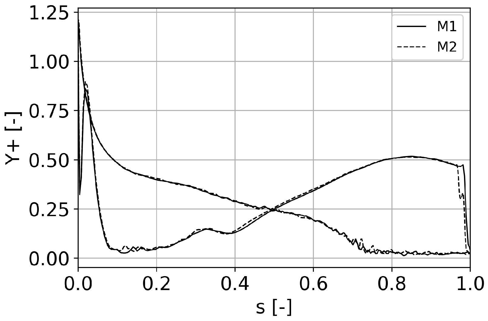
To investigate the flow sensitivity to mesh resolution, two meshes have been used, i.e., M1 and M2. The goal of these meshes is to provide a wall-resolved LES over portions of the domain where experimental data are available and feature relevant flow physics. As such, the hub wall after the tip and the blades up to about 60% of the span have a $y^{+}\le 1$, where $y^{+}$ is the wall-normal non-dimensional coordinate relative to the wall of interest. To achieve this wall resolution, six layers of prisms are used on the blade and hub wall. For both mesh M1 and M2, the first layer height is $0.0125$ mm, and a geometrical growth rate of 1.15 is applied. Figure 3 illustrates the obtained wall resolution at mid-span for both mesh M1 and M2 showing that except very close to the leading edge where $y^{+}$ reaches 1.25, $y^{+}$ is below 0.5 on a large portion of the profile.

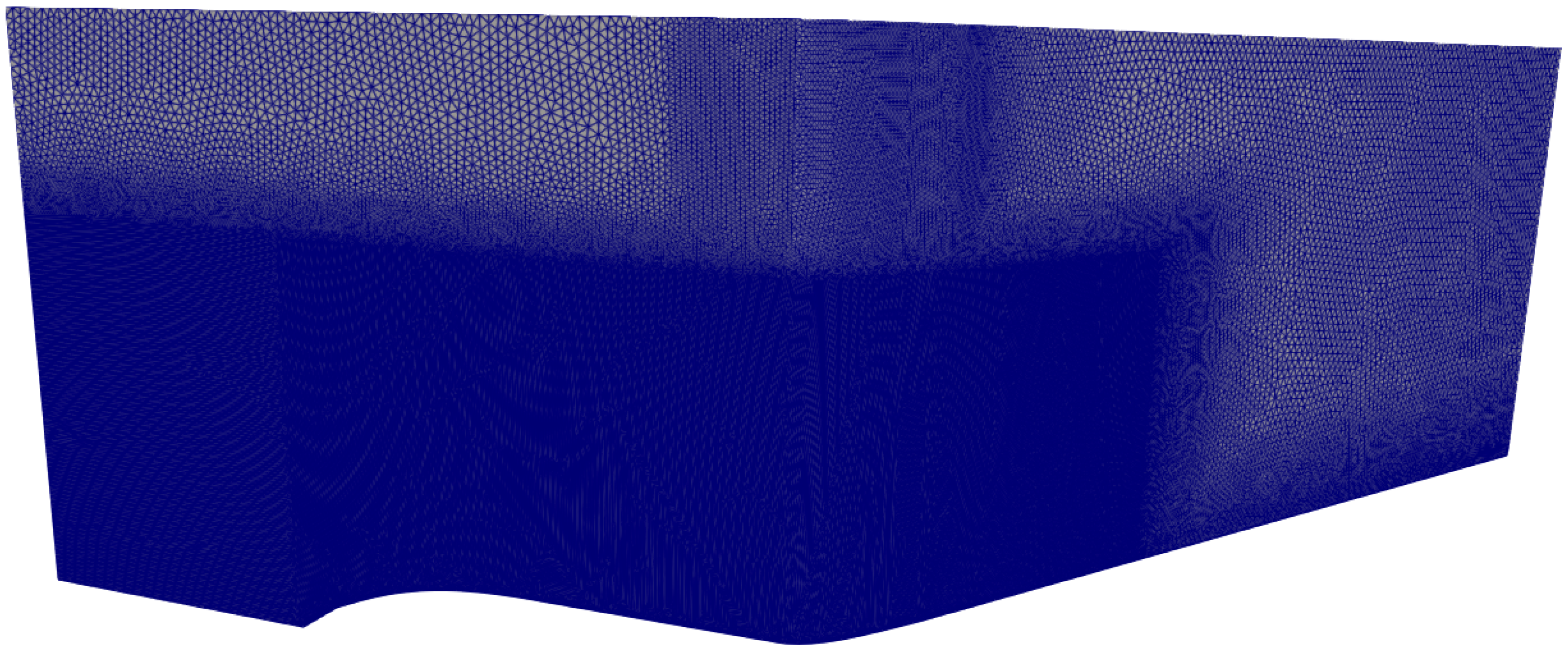
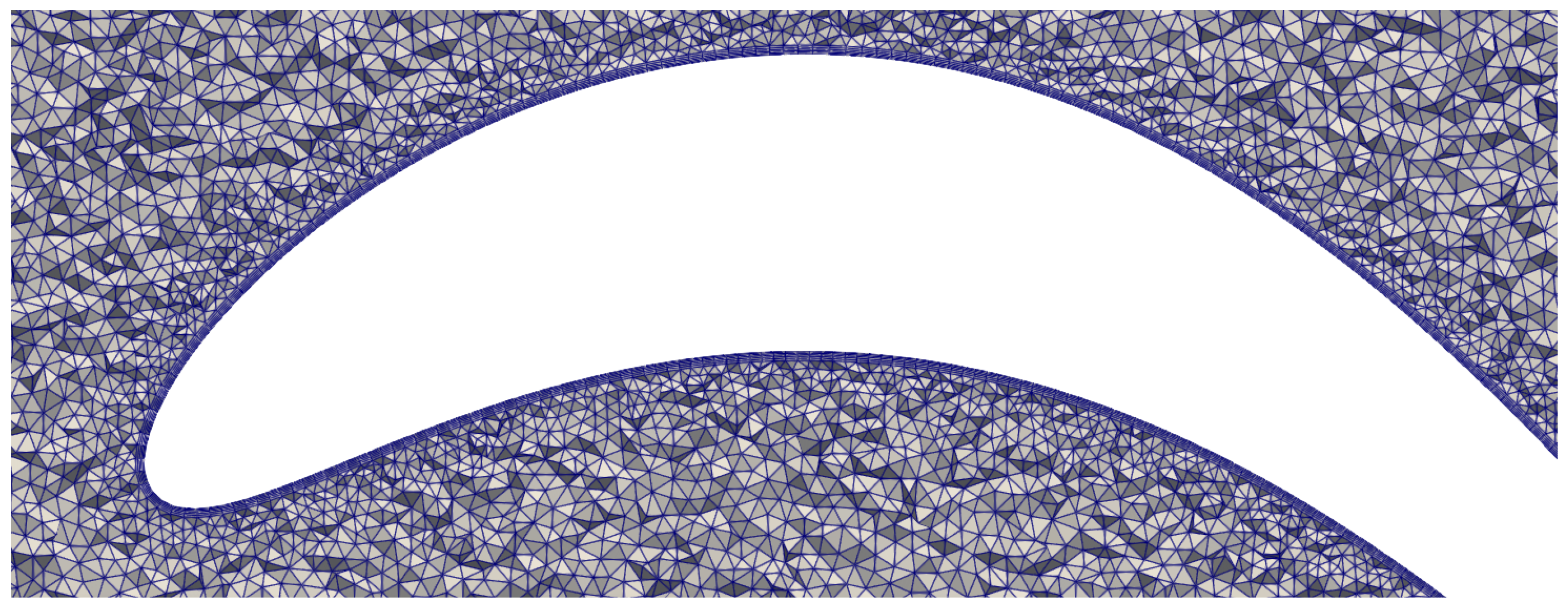
Tetrahedra are used elsewhere in the domain. The target mesh size is 2 mm except in the refined region starting from the inlet to one blade chord downstream the cascade and up to 60% of the blade span where the size is prescribed to 0.4 mm for M1 and 0.25 mm for M2 (Figure 4 and Figure 5). These resolutions are finer than in Perkins and Duchaine [21], where the transport of the injected turbulence is shown to be well captured. The resulting mesh sizes are about 90 millions cells for M1 and 220 millions cells for M2.

Table 1. Boundary conditions used in computations.

Boundary Condition	Flow Quantity Imposed	Values
Inlet	Total pressure	9000 Pa
	Total temperature	300 K
	Inlet yaw angle	40.2°
Outlet	Static pressure	5323.3 Pa
Left	Periodicity	–
Right	Periodicity	–
Shroud Wall	Slip adiabatic wall	–
Hub Wall	No-slip adiabatic wall	–
Blades	No-slip adiabatic wall	–

summaries the boundary conditions and provides values used. Both the inlet and outlet are applied using Navier–Stokes characteristic boundary conditions (NSCBC) [31,32,33]. Compared to the work of Perkins and Duchaine [21], a total pressure profile is imposed at the inlet boundary instead of a constant value. This profile has been fitted on data provided by VKI and adjusted to capture the total pressure on plane 2 in front of the blades:

$$P_{tot}=8150+850\left(1-e^{{\displaystyle \frac{-y^{*}}{0.04}}}\right)$$

(1)

with

$$y^{*}={\displaystyle \frac{y-y_{min}}{y_{max}-y_{min}}}$$

(2)

and $y_{min}$ and $y_{max}$ defined on Figure 2. At the design operating condition for the SPLEEN experimental set-up, the turbulence intensity at Plane 02 was measured to be $2.4\%$ with an integral length of 12 mm. This integral length was determined via a zero-frequency extrapolation on the velocity spectra, after filtering [34]. For the simulations presented in this paper, a synthetic turbulence injection method compliant with periodicity condition is used [35]. The simulated turbulent spectrum is a Passot–Pouquet spectrum [36] described by the integral length, $L_i=12\mathrm{mm}$, the velocity rms, $U_{rms}=2.4\mathrm{m}.{\mathrm{s}}^{-1}$, and by the cutoff length, $L_c=1\mathrm{mm}$.

The hub and blade walls are considered to be adiabatic no-slip walls, while the shroud wall is treated as a slip adiabatic wall. The sides of the simulated domain in the z direction have periodicity conditions imposed.

To assess the reliability of the numerical setup, a total of 5 simulations are presented in this paper depending on the mesh used and numerical scheme as well as inlet profile of total pressure. M1-LW and M2-LW refer to the simulations using the LW scheme with meshes M1 and M2, respectively, along with inlet total pressure profile. In a similar way, M1-TG and M2-TG refer to the simulations performed with meshes M1 and M2 with the TTGA4 scheme and an inlet total pressure profile. Finally, M2-TG-NP concerns the simulation with mesh M2, TTG4A scheme with a constant totale pressure imposed at the inlet boundary.

4. Results

The results section presents first, briefly, the general flow organization around the blade illustrating that the LES is able to reproduce the expected flow features. Then, time-averaged data are used to compare the five simulated cases and assess their capability to reproduce the experimental measurements.

4.1. General Instantaneous Flow Organization

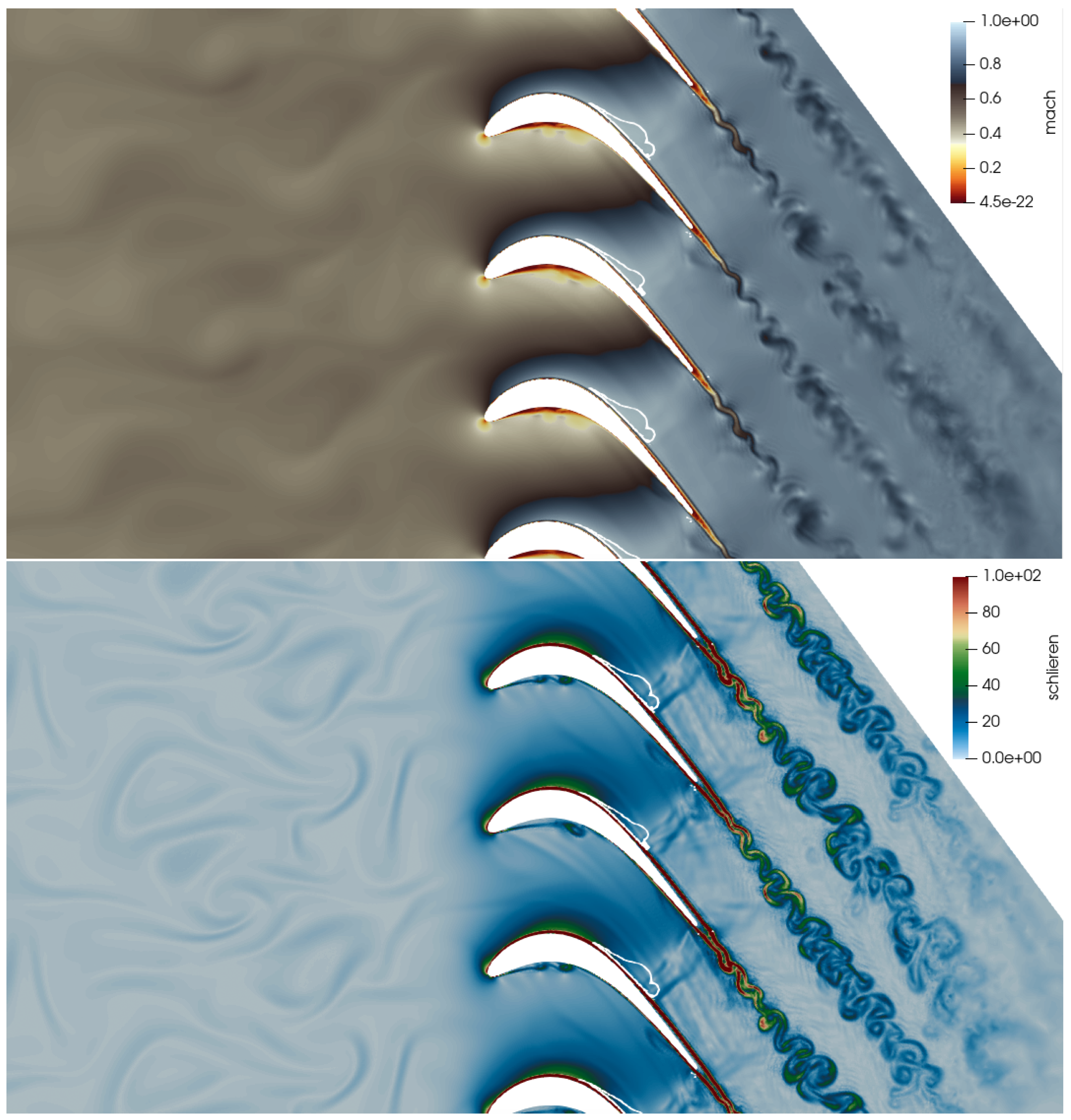
Figure 6 illustrates the instantaneous flow development around the blade profile at mid-span, representing the Mach number and a numerical Schlieren obtained with case M2-TG. Turbulent flow at about Mach 0.45 is injected in the domain. As expected, the blade induces a strong acceleration of the flow, the Mach number reaching transonic conditions illustrated by the white iso-line of Mach number equal to 1. A large unsteady separation occurs on the pressure side close to the leading edge. The boundary layers remain laminar on both the suction and pressure sides. The suction side boundary layer separates after the shock without transitioning to turbulence and without reattaching before the trailing edge. Finally, an unsteady shedding wake develops downstream of the blade.

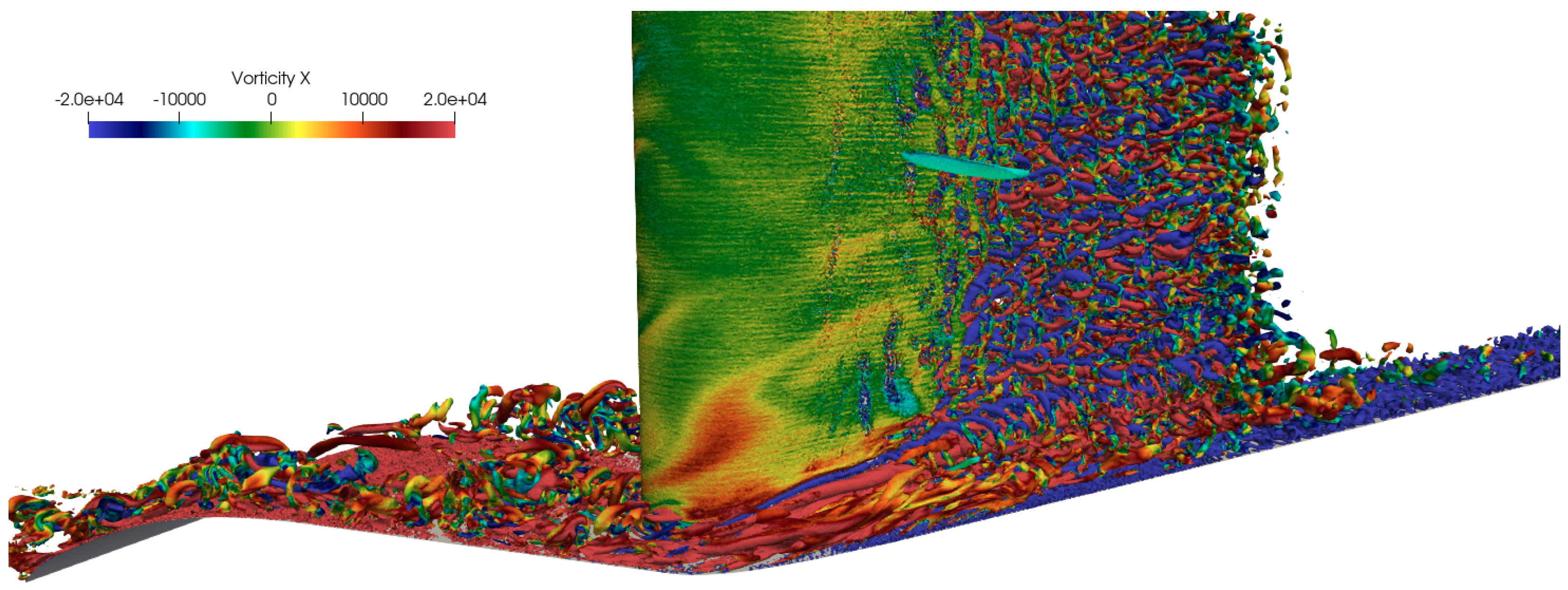
The complexity of the instantaneous turbulent flow field close to the hub is illustrated in Figure 7, which presents an iso-surface of Q-criterion colored by the axial vorticity. A turbulent boundary layer is developing on the hub before reaching the bladed leading edge. The interaction of this boundary layer with the blade generates well-known secondary flows such as horseshoe, passage, corner, and trailing shed vortices responsible of losses.

4.2. Time-Averaged Flow Features

The comparison of the five cases starts with the prediction at the inlet of the cascade (Plane 02 in front of the blades), followed by the flow field around the blade and then the losses quantification at the outlet of the cascade (Plane 06). All the simulations have been time-averaged on more than 30 flow passages around the blade, the flow passage time being evaluated based on the inlet velocity and blade chord. Convergence of the simulations was assessed with the LW scheme on both M1 and M2 meshes, computing a total of 100 characteristic convective times. No major modification of the statistics of interest was observed when increasing the averaging time above 30 convective times. A convective time is performed in less than 800 CPU hours for M1 and 2400 CPU hours for M2 when the 3rd-order TTG4A numerical scheme is used on AMD Rome cores (2.6 GHz). These times have to be divided by a factor of two for the 2nd-order LW numerical scheme.

4.2.1. Flow Prediction at the Inlet of the Cascade

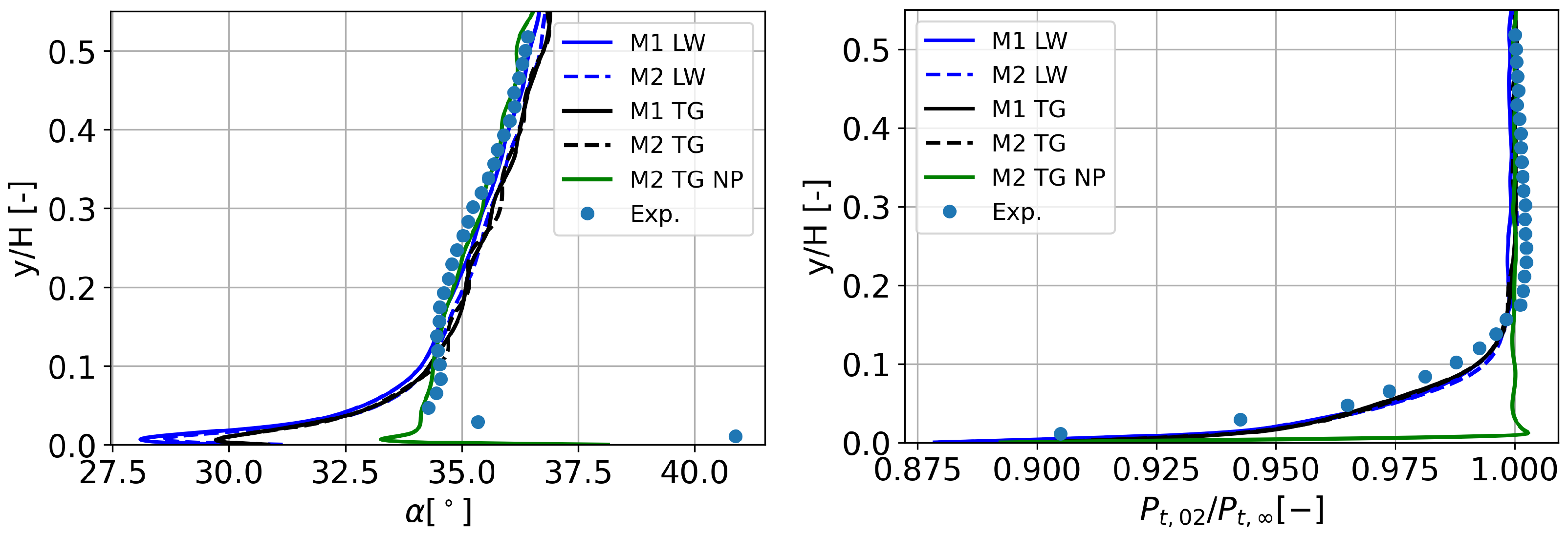
Figure 8 presents the profiles of the time and pitch averaged yaw angle $\alpha =arctan(v_z/v_x)$ along with the ratio of the total pressure at Plane 02 $P_{t,02}$ scaled by the reference infinite total pressure $P_{t,\infty }=9000$ Pa. Due to the geometrical contraction in the y direction from the inlet to Plane 02, the flow accelerates in the axial direction modifies the yaw angle. Simulations M1-LW, M2-LW, M1-TG, and M2-TG are in good accordance with the experimental measurements except close to the hub wall, where the numerical predictions are too low. Conversely, case M2-TG-NP leads to an almost perfect match with the experimental yaw angle. Concerning the total pressure profile, the results obtained with cases where a profile is used at the inlet (M1-LW, M2-LW, M1-TG, and M2-TG) show as expected a good match with the experimental data while the case without inlet total pressure profile M2-TG-NP exhibits a too thin boundary layer. It is important to remember that the results of Perkins and Duchaine [21], which include the full hub geometry and no pressure profile at the inlet, lead to a too thin boundary layer, which can be corrected by an inlet profile of total pressure, as well as a badly predicted yaw angle profile ranging from 27° to almost 40° on the region of interest.

4.2.2. Flow Prediction in the Cascade Passage

The blade loadings are presented on Figure 9 at $y/H$ = 4% and $y/H$ = 50% for the different cases. At mid-span, all the simulations provide almost the same results in good accordance with the experimental measurements. It is shown that all the numerical modeling seem to provide a too-long recirculation zone on the pressure side close to the leading edge, the more accurate results being obtained with the M2-TG setup. Concerning the position close to the hub, at $y/H$ = 4%, all the cases with the total pressure inlet profile lead to almost the same loading on the blade in good accordance with the experimental results. The case M2-TG-NP with a constant total pressure at the inlet leads to a higher loading due to the fact the total pressure at $y/H$ = 4% is higher than expected (Figure 8).

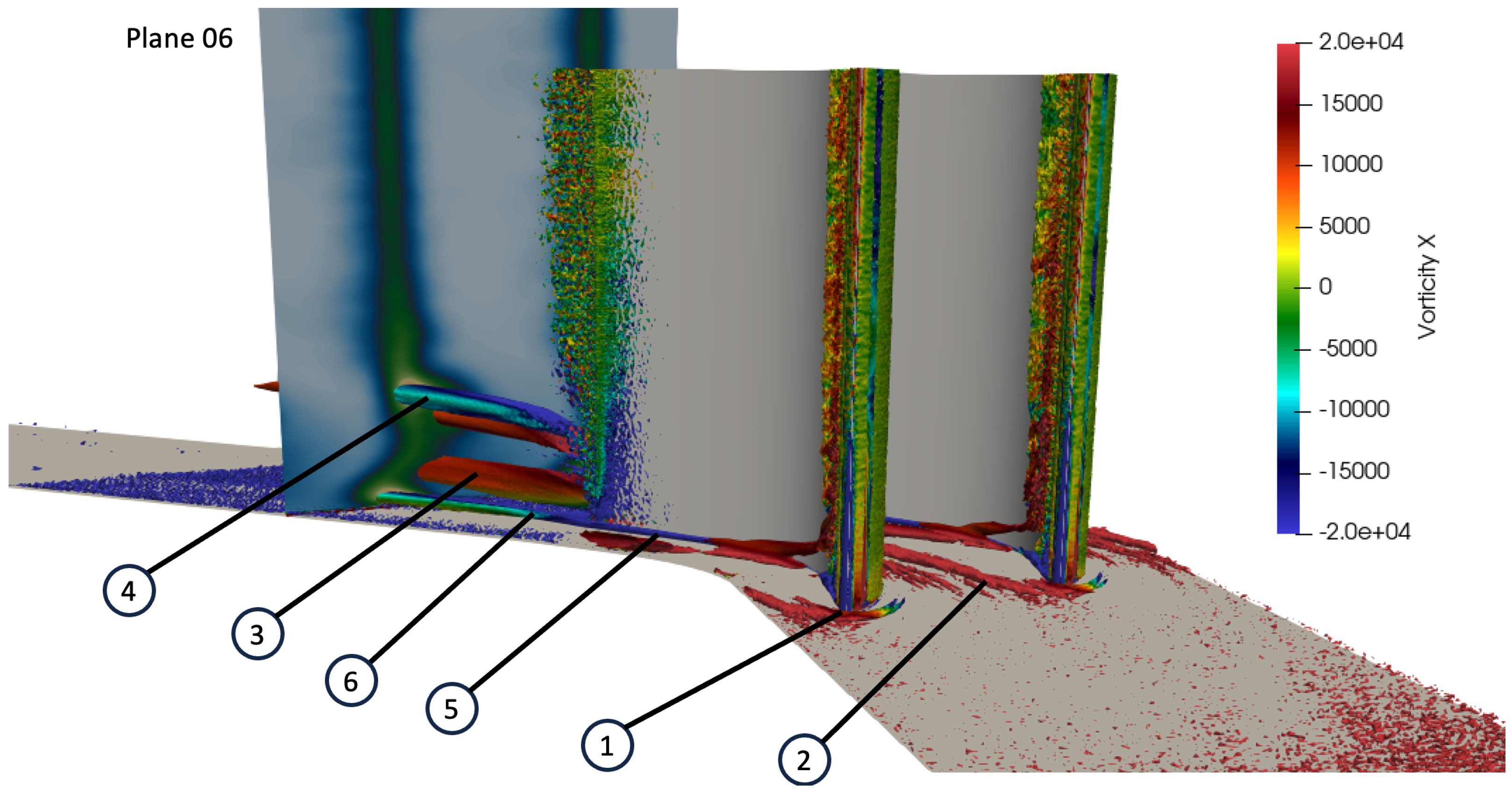
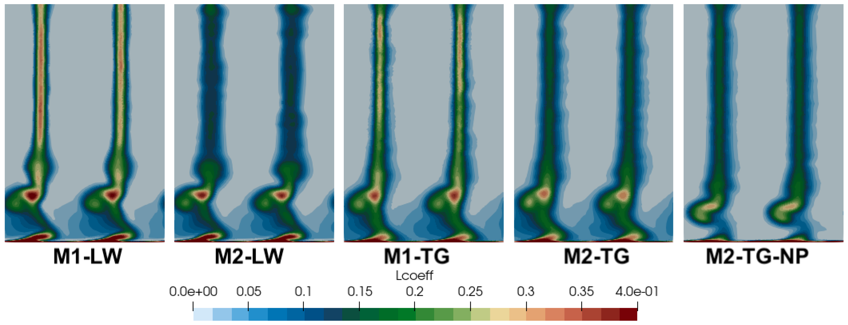
The focus of the analysis in this paper is secondary losses, which refers to the losses generated from the processes related to the interaction of the hub boundary layer and the blades. To investigate the differences between the simulated cases, the identification of secondary flow close to the hub is performed [37]. Figure 10 presents an iso surface of Q-criterion $Q=5\times {10}^7{s}^{-2}$ based on a time-averaged field obtained with M2-TG. The first secondary flow structure to develop is the horseshoe vortex (labeled 1), issued from the interaction between the incoming boundary layer and the blade leading edge due to a high pression region and roll up of the boundary layer. This horseshoe vortex travels down the blade passage, and the vortex generated on the pressure side is pulled by the pressure gradient towards the suction side of the nearby blade (label 2). The suction leg of the horseshoe vortex and the other shed pressure leg merge in the blade passage, forming the passage vortex (label 3). This strong passage vortex induces several other smaller vortices, notably the wall-induced vortex (label 4) and the suction-side corner vortex (label 6). A pressure-side corner vortex is also visible on the image (label 5). The five simulations with different mesh resolutions, numerical schemes and inlet conditions lead to different organizations of secondary flow structures in terms of vortex positioning, intensity and fluctuations. This is illustrated on Figure 11 which displays the turbulent kinetic energy (TKE) on Plane 06 downstream of the blade, from the hub to $y/H=60\%$ (i.e., in the refined region). This figure evidences the higher turbulence generated in the blade wake as well as the footprint of the secondary flow structures. A first core of high TKE (C1) corresponds to the passage and wall-induced vortex at around $y/H=10\%$ and the second (C2) close to the hub corresponds to the corner vortex. Comparing the cases, it is evident that the mesh resolution plays a critical role on the resolved TKE in the wake above $y/H=20\%$ as well as in the cores linked to the secondary vortices: as mesh resolution increases from M1 to M2, more TKE is predicted in the wakes and vortex induced cores. Whatever the mesh resolution and numerical scheme (M1-LW, M2-LW, M1-TG, and M2-TG), the secondary flows are located at the same spanwise y and transversal z location. Nonetheless, the second-order numerical scheme LW predicts higher levels of TKE in the first core C1 compared to the higher-order scheme TTG4A, the opposite being observed in the second core. The cases M1-LW and M2-LW also predict a third core of lesser intensity located just above C1, not predicted the other simulations. Finally, when it comes to the simulation with a constant inlet total pressure M2-TG-NP, the higher total pressure close the hub leads to the development of passage and induced vortices closer to the hub than in the corresponding case with an inlet total pressure profile (M2-TG).

To compare and characterize how these flow features affect losses, the energy loss coefficient $\xi$ computed at Plane 06 downstream of the blade is used [12]. It is expressed as:

$$\xi (y,z)=1-{\displaystyle \frac{1-{\left(\frac{P_6(y,z)}{P_{06}(y,z)}\right)}^{\frac{\gamma -1}{\gamma }}}{1-{\left(\frac{P_6(y,z)}{P_{01,fs}}\right)}^{\frac{\gamma -1}{\gamma }}}}$$

(3)

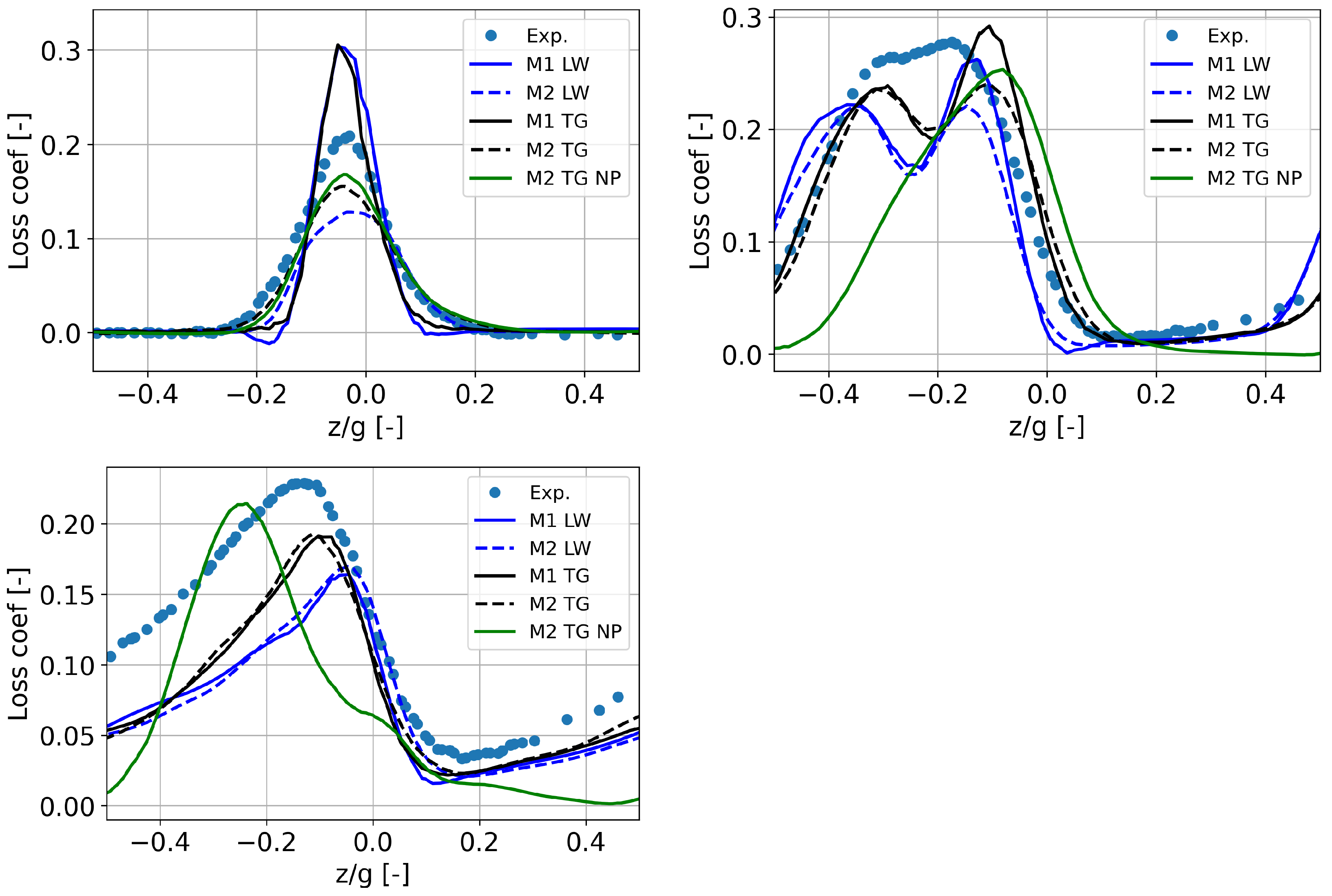
where $P_6(z,y)$ is the local static pressure at Plane 06 and $P_{06}(y,z)$ is the local total pressure at Plane 06. $P_{01,fs}$ is the mean freestream total pressure at Plane 01 upstream of the blade, here taken to be the imposed total pressure at the inlet, 9000 Pa. $\gamma$ is the ratio of specific heats for air, taken as $\gamma =1.4$. This coefficient is useful as it contextualizes the losses, which manifest as a decrease in total pressure at Plane 06. Figure 12 shows the contours of the pressure loss coefficient at Plane 06 for the five simulated cases. In all cases, the main loss region originates from the wakes of the blades and the interaction of these wakes with the secondary flow vortices. As evidenced with the TKE, two regions with increased losses can be identified, one between the interaction of the passage vortex and the wall-induced vortex (C1), and the other near the corner vortex (C2). The case M2-TG-NP exhibit as expected a slightly different distribution of these cores close to the hub compared to the other cases. Mesh resolution and numerical scheme plays an important role in the predicted losses. Increasing mesh resolution from M1 to M2 first leads to a decrease in intensity of the peak of losses in the wake region above $y/H=20\%$ along with a wider loss spread in the blade to blade direction. It also leads to a decrease in the loss intensity in the cores associated with secondary vortices. The effect of increasing the numerical scheme accuracy from LW to TTG4A is not evident and is further analyzed by comparing the pressure loss coefficient $\xi$ at different spans compared to experimental measurements. Figure 13 presents the profiles of pressure loss coefficient $\xi \left(z\right)$ at $y/H=4\%$, $y/H=10\%$ and $y/H=50\%$ for the five cases. In the wake region $y/H=50\%$, the finer grid along with the higher order numerical scheme (M2-TG) provides better results in terms of intensity of the losses as well as spread of the wake region. At $y/H=10\%$, the topology of the pressure loss coefficient is rather complex and once again, the case M2-TG leads to the better results, indicating its capability to well reproduce the position and intensity of the secondary vortices. Finally, closer to the hub at $y/H=4\%$, although the agreement with experimental data is lesser, the setup M2-TG provides the more accurate results. It is also evident from these results that the imposition of a constant total pressure at the inlet leads to inaccurate results in terms of secondary flow positioning and intensity.

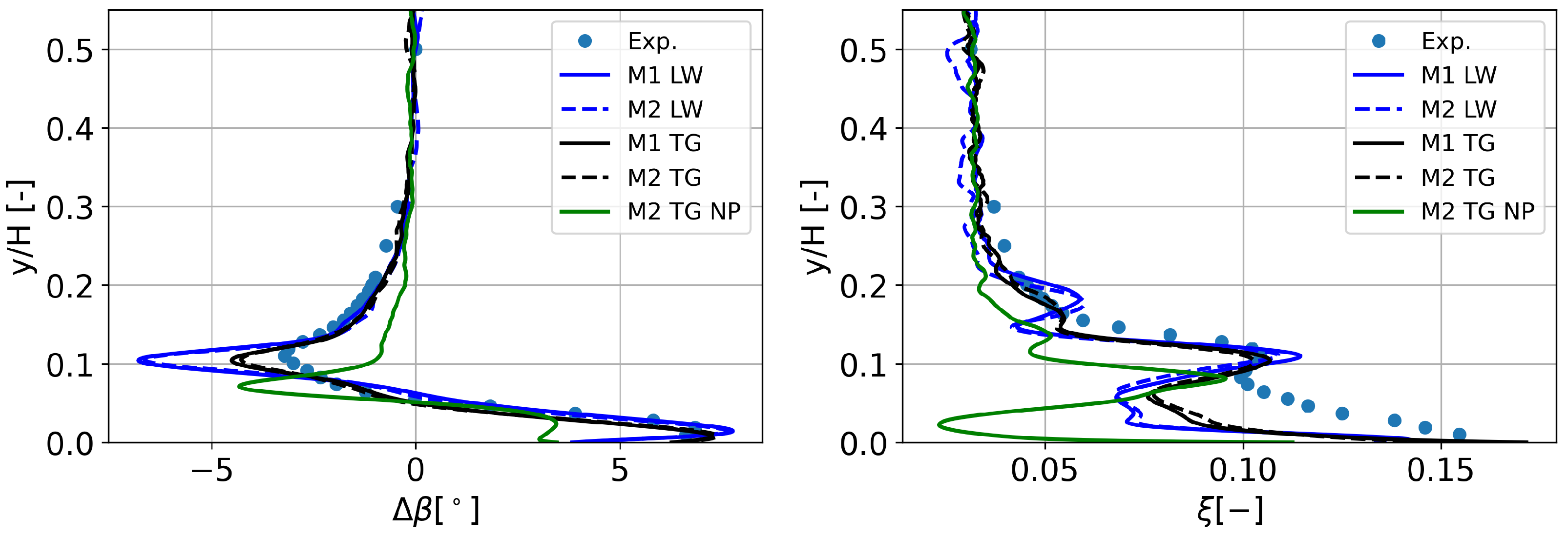
To finalize the comparisons, the time- and pitch-averaged deviations to the turning angle and pressure loss coefficient on Plane 06 for the five cases are compared to experimental data. The turning angle is defined as

$$\mathrm{\Delta }\beta =arctan\left({\displaystyle \frac{v_z}{v_x}}\right)-{\beta }_{m,out},$$

(4)

where ${\beta }_{m,out}=56.7$ is the deviation angle imposed by the blade. Note that both the deviation angle and pressure loss coefficient are mass averaged when it comes for the spatial averaging in the pitchwise direction. Figure 14 presents the spanwise profiles of $\mathrm{\Delta }\beta$ and $\xi$, showing the overall effects of the secondary structures from the different cases relative to experimental data. The best agreement for both the turning angle and pressure loss coefficient is obtained with the M2-TG setup. The position and intensity of the overturning close to the hub and under-turning close to $y/H=10\%$ associated with the secondary flow patterns are well recovered. Concerning the pressure loss coefficient, a very good match is observed except close to the wall where the losses are underestimated by all the setups. The cases with the LW numerical scheme show acceptable results but with a less good accuracy compared to TTG4A. The peak of pressure loss coefficient evidenced in Figure 12 close to $y/H=20\%$ is clearly seen on the $\xi$ profile when the LW scheme is used. Figure 14 illustrates as expected from Figure 12, that the case with the constant inlet total pressure M2-TG-NP badly predicts the position and intensity of both quantities $\mathrm{\Delta }\beta$ and $\xi$ due to the development of secondary flows too close to the hub wall. Finally, it is worth mentioning that although the profiles of pressure loss coefficient in the wake region $y/H=50\%$ presented in Figure 13 are different between the LW and TTG4A schemes, almost the same pitchwise integrated values are obtained illustrating that comparing local information is of paramount importance to evaluate the accuracy of the numerical methods used.

4.3. Loss Quantification in the Flow Passage

The previous section demonstrated that the setup M2-TG, relying on the most refined grid and the higher order numerical scheme TTG4A along with an inlet total pressure profile, provides accurate results compared to available experimental measurements. This setup is thus used to quantify loss generation in the cascade. To do so, the time-average dissipation rate (loss in kinetic energy):

$$LIKE=\overline{(\mu +{\mu }_t){\left({\displaystyle \frac{\partial u_i}{\partial x_j}}+{\displaystyle \frac{\partial u_j}{\partial x_i}}\right)}^2}$$

(5)

and the turbulent kinetic energy dissipation rate:

$$ϵ=\overline{(\mu +{\mu }_t){\left({\displaystyle \frac{\partial u_i^{\prime }}{\partial x_j}}+{\displaystyle \frac{\partial u_j^{\prime }}{\partial x_i}}\right)}^2}$$

(6)

are estimated in the simulation. In Equations (5) and (6), $\mu$ is the dynamic viscosity, subscript t refers to the sub-grid scale quantity, $u_i$ is the instantaneous velocity vector in direction i, and $u_i^{\prime }$ is its fluctuation component. The turbulent kinetic energy dissipation rate is estimated based on the dissipation of the mean kinetic energy ($DMKE$) such that $ϵ=LIKE-DMKE$.

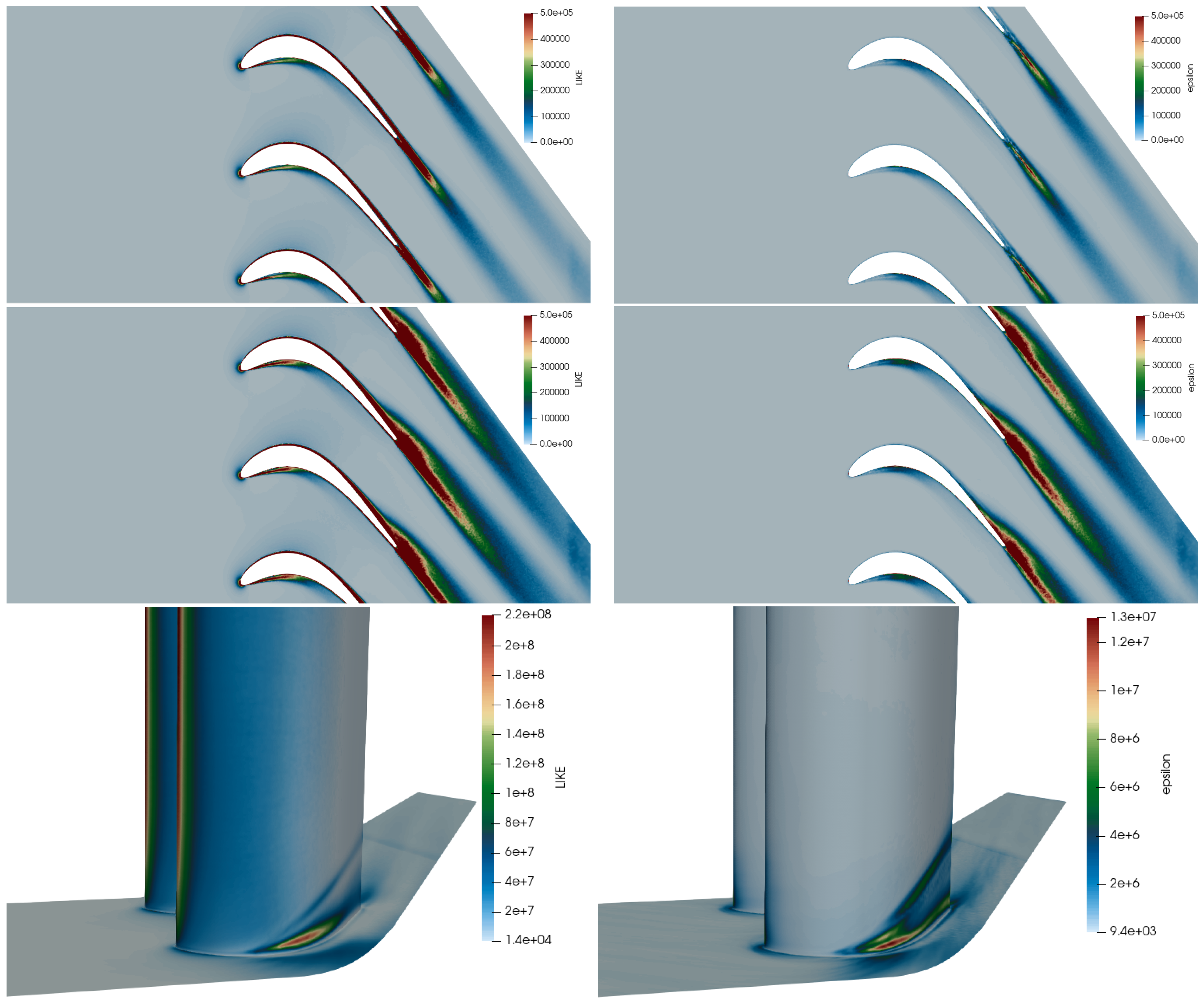
Figure 15 shows the distribution of LIKE and $ϵ$ at mid-span, $y/H=10\%$, and on the walls of the configuration. At mid-span, losses are mainly generated around the blade profile and in the wake. The dissipation of the mean kinetic energy produces high levels of LIKE in the leading edge region, pressure-side separation bubble, all along the pressure and suction side laminar boundary layers, and in the wake. The turbulent dissipation rate $ϵ$ mainly contributes to losses in the transition region of the pressure-side separated bubble as well as in the wake of the blade. At $y/H=10\%$, the contribution of secondary flows to losses is clearly identified by high levels of LIKE in the trailing edge region as well as in the wake. In these regions, the turbulent dissipation rate $ϵ$ contributes to a large extent to the losses in kinetic energy. The distributions of LIKE and $ϵ$ on the blade walls illustrate, first, the important dissipation due to the mean field close to leading edge on the suction side: the strong acceleration along with the thin boundary layer lead to high levels of LIKE in this region. The footprints of secondary vortices are also clearly visible downstream on the suction side: the high levels of both LIKE and $ϵ$ close to the hub are linked to the impact of the passage vortex emanating from the pressure-side leg of the horseshoe vortex of the adjacent blade. The trajectory of the induced wall vortex is also visible, originating close to the impingement region of the passage vortex on the suction side and then migrating towards higher $y/H$ downstream.

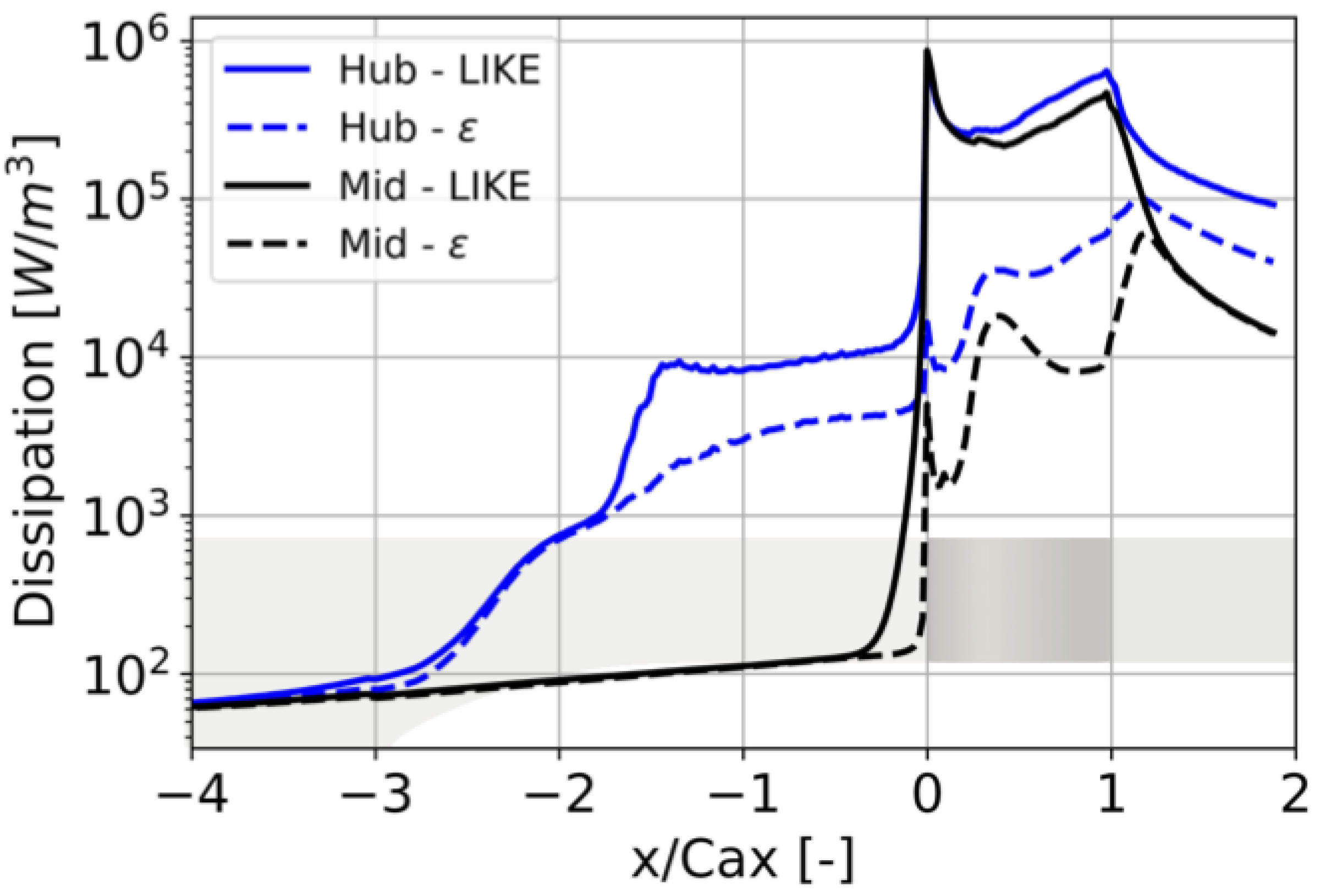
Finally, Figure 16 presents the axial evolution of the volume average LIKE and $ϵ$ on small sections along the configuration of the hub and mid-vein regions. The hub region ranges from $y=0$ and $y/H=25\%$, including all the locations where the secondary flows develop. The mid-vein region starts at $y/H=25\%$ and continues to $y/H=50\%$. The axial coordinate is scaled by the blade axial chord $C_{ax}$, the leading edge being at $x/C_{ax}=0$ and thus, the trailing edge being at $x/C_{ax}=1$. In the mid-vein section, LIKE and $ϵ$ are almost equal from upstream of the boundary layer lip until $x/C_{ax}=-0.3$, just upstream of the blade. In this region, the dissipation is mainly due to the turbulent eddies injected at the inlet of the domain with a very small effect of the acceleration due to the contraction of the domain in the y direction. As illustrated in Figure 15, the deviation of the flow linked to the blade profile induces the highest levels of dissipation in LIKE in the domain, also evidenced in Figure 16 at $x/C_{ax}=0$. As the flow passes the leading edge, turbulent fluctuations are generated increasing the turbulent dissipation rate $ϵ$. This later increases due to the transition of the separated bubble on the pressure side and decreases after reattachment and relaminarization of the boundary layer. The level of LIKE is always higher than $ϵ$ by more than an order of magnitude due to wall friction and dissipation linked to the mean flow field. Due to the turbulent wake development, $ϵ$ increase downstream from $x/C_{ax}=1$ to reach a maximum around $x/C_{ax}=1.25$. Downstream of this maximum, LIKE and $ϵ$ are almost equal, indicating that losses are mainly due to turbulent mixing in this region. From $x/C_{ax}=-4$ to −3, the dissipations in the hub and mid-vein regions show similar levels. Downstream of $x/C_{ax}=-3$ up to −1.75, the contraction of the flow in the y direction linked to the boundary layer trip induces an acceleration of the flow mainly in the hub region, leading to a progressive increase of the losses. At $x/C_{ax}=-1.75$, the volume where the average is made intersects the hub wall, leading to a sharp increase of LIKE with respect to $ϵ$ as the friction at the wall is accounted for. In the blade region, from $x/C_{ax}=0$ to 1, both LIKE and $ϵ$ show higher levels in the hub part than in the mid-vein one due to the secondary flow development leading to an increase of wall friction as well as the generation of more turbulence (higher $ϵ$). These higher levels of dissipation are still present downstream of the blade as the secondary structures are still not fully dissipated ($ϵ$ higher in the hub part than mid-vein) and due to wall friction at the hub. When integrating loss sources in the hub and vein domains, the results show that approximately 62% of the total losses (i.e., integration of LIKE) are generated in the hub region. The turbulent dissipation represents around 18% of the losses in the hub region and 10% in the mid-vein region.

5. Conclusions

A high-fidelity numerical setup is proposed to simulate the SPLEEN cascade representative of a high-speed, low-pressure turbine blade. The effects of mesh resolution, numerical scheme accuracy, and inlet total pressure profile on the flow field development and prediction of losses in a case without wake generator and purge flow at outlet Reynolds and Mach numbers of 70,000 and 0.9, respectively, are investigated in the context of wall-resolved large-eddy simulation. It is shown that the inlet total pressure profile plays a critical role in the development of the secondary flow structure and associated losses; imposing a relevant profile is thus important. The results also illustrate that the blade loading results are robust to the mesh resolution and numerical scheme. Nonetheless, the accuracy and quality of the numerics are decisive when it comes to the prediction of the secondary flow and wake development and associated losses. The most refined mesh and higher-order numerical scheme are mandatory to reproduce the experimental results downstream of the cascade. Based on the best numerical LES setup, the generation of losses in the hub and mid-vein regions are analyzed. This shows that approximately 62% of the total losses are generated in the hub region and that the turbulent dissipation represents around 18% of the losses in the hub region and 10% in the mid-vein region.

References

1. Duchaine, F.; Delon, X. Assessment of Large-Eddy Simulations to simulate a high-speed low-pressure turbine cascade. In Proceedings of the 16th European Conference on Turbomachinery Fluid dynamics & Thermodynamics, Hannover, Germany, 24–28 March 2025. Number ETC2025-292. [Google Scholar]
2. Kurzke, J. Fundamental Differences Between Conventional and Geared Turbofans. In Turbo Expo: Power for Land, Sea, and Air; American Society of Mechanical Engineers: New York, NY, USA, 2009; Volume 1, pp. 145–153. [Google Scholar] [CrossRef]
3. Kestner, B.K.; Schutte, J.S.; Gladin, J.C.; Mavris, D.N. Ultra High Bypass Ratio Engine Sizing and Cycle Selection Study for a Subsonic Commercial Aircraft in the N+2 Timeframe. In Turbo Expo: Power for Land, Sea, and Air; American Society of Mechanical Engineers: New York, NY, USA, 2011; Volume 1, pp. 127–137. [Google Scholar] [CrossRef]
4. Johnson, B.V. Internal Air and Lubrication Systems. In Encyclopedia of Aerospace Engineering; John Wiley & Sons, Ltd.: Hoboken, NJ, USA, 2010. [Google Scholar] [CrossRef]
5. Steiner, M.; Zerobin, S.; Bauinger, S.; Heitmeir, F.; Göttlich, E. Development and Commissioning of a Purge Flow System in a Two Spool Test Facility. In Proceedings of the 12th European Conference on Turbomachinery Fluid Dynamics & Thermodynamics, Stockholm, Sweden, 3–7 April 2017; pp. 3–7. [Google Scholar]
6. Moore, A. Gas Turbine Engine Internal Air Systems: A Review of the Requirements and the Problems. In Turbo Expo: Power for Land, Sea, and Air; American Society of Mechanical Engineers: New York, NY, USA, 1975; p. V001T01A001. [Google Scholar] [CrossRef]
7. Giovannini, M.; Rubechini, F.; Marconcini, M.; Arnone, A.; Bertini, F. Analysis of a LPT Rotor Blade for a Geared Engine: Part I — Aero-Mechanical Design and Validation. In Turbo Expo: Power for Land, Sea, and Air; American Society of Mechanical Engineers: New York, NY, USA, 2016; Volume 2B, p. V02BT38A053. [Google Scholar] [CrossRef]
8. Pau, M.; Paniagua, G.; Delhaye, D.; de la Loma, A.; Ginibre, P. Aerothermal Impact of Stator-Rim Purge Flow and Rotor-Platform Film Cooling on a Transonic Turbine Stage. J. Turbomach. 2010, 132, 021006. [Google Scholar] [CrossRef]
9. Léonard, T.; Gicquel, L.; Gourdain, N.; Duchaine, F. Steady/Unsteady Reynolds-Averaged Navier–Stokes and Large Eddy Simulations of a Turbine Blade at High Subsonic Outlet Mach Number. J. Turbomach. 2014, 137, 041001. [Google Scholar] [CrossRef]
10. Troth, L.M.S. Multiphysics Coupled Simulations of Gas Turbines. Ph.D. Thesis, Institut National Polytechnique de Toulouse, Toulouse, France, 2017. [Google Scholar]
11. Fiore, M.; Gourdain, N.; Boussuge, J.; Lippinois, E. Delineating Loss Sources Within a Linear Cascade With Upstream Cavity and Purge Flow. J. Turbomach. 2019, 141, 091008. [Google Scholar] [CrossRef]
12. Denton, J.D. Loss Mechanisms in Turbomachines. In Turbo Expo: Power for Land, Sea, and Air; American Society of Mechanical Engineers: New York, NY, USA, 1993; Volume 2, p. V002T14A001. [Google Scholar] [CrossRef]
13. Gallier, K.D.; Lawless, P.B.; Fleeter, S. Development of the Unsteady Flow on a Turbine Rotor Platform Downstream of a Rim Seal. In Turbo Expo: Power for Land, Sea, and Air; American Society of Mechanical Engineers: New York, NY, USA, 2004; Volume 5, pp. 939–947. [Google Scholar] [CrossRef]
14. Schäflein, L.; Janssen, J.; Brandies, H.; Jeschke, P.; Behre, S. Influence of Purge Flow Injection on the Performance of an Axial Turbine With Three-Dimensional Airfoils and Non-Axisymmetric Endwall Contouring. J. Turbomach. 2022, 145, 061004. [Google Scholar] [CrossRef]
15. Hodson, H.P.; Howell, R.J. Bladerow Interactions, Transition, and High-Lift Aerofoils in Low-Pressure Turbines. Annu. Rev. Fluid Mech. 2005, 37, 71–98. [Google Scholar] [CrossRef]
16. Fard Afshar, N.; Kozulovic, D.; Henninger, S.; Deutsch, J.; Bechlars, P. Turbulence Anisotropy Analysis at the Middle Section of a Highly Loaded 3D Linear Turbine Cascade Using Large Eddy Simulation. J. Glob. Power Propuls. Soc. 2023, 7, 71–84. [Google Scholar] [CrossRef] [PubMed]
17. Boudin, A.; Dombard, J.; Duchaine, F.; Gicquel, L.; Odier, N.; Lavagnoli, S.; Lopes, G.; Simonassi, L. Analysis of rotor/stator interactions in a high-speed low-pressure turbine cascade using Large-Eddy Simulations. In Proceedings of the 15th European Conference on Turbomachinery Fluid dynamics & Thermodynamics, Budapest, Hungary, 24–28 April 2023. Number ETC2023-257. [Google Scholar]
18. Hullin, L.; Gonzalez-Martino, I.; Bonnal, B. Unsteady Flow Simulations of a Transonic Low-Pressure Turbine Cascade. In Turbo Expo: Power for Land, Sea, and Air; American Society of Mechanical Engineers: New York, NY, USA, 2024; Volume 12B. [Google Scholar]
19. Tene Hedje, P.; Bechane, Y.; Lavagnoli, S.; Bricteux, L. Wall Resolved Large-Eddy Simulations of High-Speed Low-Pressure Turbine Cascades. In Turbo Expo: Power for Land, Sea, and Air; American Society of Mechanical Engineers: New York, NY, USA, 2023; Volume 13B, p. V13BT30A005. [Google Scholar]
20. Tene Hedje, P.; Bricteux, L.; Bechane, Y.; Lavagnoli, S. Large Eddy Simulations of a High-Speed Low-Pressure Turbine Cascade at Subsonic and Transonic Mach Numbers. In Turbo Expo: Power for Land, Sea, and Air; American Society of Mechanical Engineers: New York, NY, USA, 2024; Volume 12C. [Google Scholar]
21. Perkins, D.W.; Duchaine, F. Large-Eddy Simulations of a High-Speed Low-Pressure Turbine Cascade With Purge Flow. In Turbo Expo: Power for Land, Sea, and Air; American Society of Mechanical Engineers: New York, NY, USA, 2024; Volume 12C. [Google Scholar]
22. Lavagnoli, S.; Lopes, G.; Simonassi, L.; Torre, A.F.M. SPLEEN-High Speed Turbine Cascade—Test Case Database; Zenodo: Geneva, Switzerland, 2023. [Google Scholar] [CrossRef]
23. Okada, M.; Simonassi, L.; Lopes, G.; Lavagnoli, S. PIV Measurements in a High-Speed Low-Reynolds Low-Pressure Turbine Cascade. In Proceedings of the ASME Turbo Expo 2023: Turbomachinery Technical Conference and Exposition, Boston, MA, USA, 26–30 June 2023. GT2023-102156. [Google Scholar]
24. Pastorino, G.; Simonassi, L.; Lopes, G.; Boufidi, E.; Fontaneto, F.; Lavagnoli, S. Measurements of Turbulence in compressible Low-Density Flows at the Inlet of a Transonic Linear Cascade with and without Unsteady Wakes. J. Turbomach. 2024, 146, 071002. [Google Scholar] [CrossRef]
25. Lopes, G.; Simonassi, L.; Lavagnoli, S. Time-Averaged Aerodynamics of a High-Speed Low-Pressure Turbine Cascade with Cavity Purge Flow and Unsteady Wakes. J. Turbomach. 2024, 146, 021008. [Google Scholar] [CrossRef]
26. Lax, P.; Wendroff, B. Systems of Conservation Laws. Commun. Pure Appl. Math. 1960, 13, 217–237. [Google Scholar] [CrossRef]
27. Quartapelle, L.; Selmin, V. High-order Taylor-Galerkin methods for nonlinear multidimensional problems. Finite Elem. Fluids 1993, 76, 46. [Google Scholar]
28. Colin, O.; Benkenida, A.; Angelberger, C. 3d Modeling of Mixing, Ignition and Combustion Phenomena in Highly Stratified Gasoline Engines. Oil Gas Sci. Technol.-Rev. IFP 2003, 58, 47–62. [Google Scholar] [CrossRef]
29. Nicoud, F.; Ducros, F. Subgrid-Scale Stress Modelling Based on the Square of the Velocity Gradient Tensor. Flow Turbul. Combust. 1999, 62, 183–200. [Google Scholar] [CrossRef]
30. Dupuy, D.; Gicquel, L.; Odier, N.; Duchaine, F.; Arts, T. Analysis of the effect of intermittency in a high-pressure turbine blade. Phys. Fluids 2020, 32, 095101. [Google Scholar] [CrossRef]
31. Poinsot, T. Boundary Conditions for Direct Simulations of Compressible Viscous Flows. J. Comput. Phys. 1992, 101, 104–129. [Google Scholar] [CrossRef]
32. Granet, V.; Vermorel, O.; Léonard, T.; Gicquel, L.; Poinsot, T. Comparison of Nonreflecting Outlet Boundary Conditions for Compressible Solvers on Unstructured Grids. AIAA J. 2010, 48, 2348–2364. [Google Scholar] [CrossRef]
33. Odier, N.; Sanjosé, M.; Gicquel, L.; Poinsot, T.; Moreau, S.; Duchaine, F. A Characteristic Inlet Boundary Condition for Compressible, Turbulent, Multispecies Turbomachinery Flows. Comput. Fluids 2019, 178, 41–55. [Google Scholar] [CrossRef]
34. Roach, P. The Generation of Nearly Isotropic Turbulence by Means of Grids. Int. J. Heat Fluid Flow 1987, 8, 82–92. [Google Scholar] [CrossRef]
35. Boudin, A. Turbulence Injection Methods for Large-Eddy Simulations; Working Note; Cerfacs-ISAE SUPAERO: Toulouse, France, 2021. [Google Scholar]
36. Passot, T.; Pouquet, A. Numerical Simulation of Compressible Homogeneous Flows in the Turbulent Regime. J. Fluid Mech. 1987, 181, 441–466. [Google Scholar] [CrossRef]
37. Langston, L.S. Secondary Flows in Axial Turbines—A Review. Ann. N. Y. Acad. Sci. 2001, 934, 11–26. [Google Scholar] [CrossRef] [PubMed]
Figure 1. Wind tunnel test section cross-section [25].
Ijtpp 10 00021 g001
Figure 2. Visualization of Perkins and Duchaine geometry (left) and present geometry (right).
Ijtpp 10 00021 g002
Figure 3. Wall resolution in non-dimensional coordinate y + for the two meshes M1 and M2 along the reduced abscissa s. s = 0 corresponds to the blade leading edge end s = 1 to the trailing edge.
Ijtpp 10 00021 g003
Figure 4. Global visualisation of mesh M2.
Ijtpp 10 00021 g004
Figure 5. A crinkle-slice focused on one of the blades at y / H = 50 % for mesh M2, zoomed out.
Ijtpp 10 00021 g005
Figure 6. Instantaneous Mach number and Schlieren contours at mid-span of the cascade for case M2-TG. Iso-line of Mach = 1.
Ijtpp 10 00021 g006
Figure 7. Q criterion colored by the axial vorticity.
Ijtpp 10 00021 g007
Figure 8. Yaw angle α and normalized total pressure profile P t , 02 / P t , at the inlet cascade Plane 02.
Ijtpp 10 00021 g008
Figure 9. Profile of isentropic Mach number along the blade profile at y / H = 4% (left) and y / H =50% (right).
Ijtpp 10 00021 g009
Figure 10. Mean Q criterion colored by axial vorticity (case M2-TG).
Ijtpp 10 00021 g010
Figure 11. TKE on Plane 06 downstream of the blades, view from downstream towards upstream.
Ijtpp 10 00021 g011
Figure 12. Pressure loss coefficient ξ on Plane 06 downstream of the blades, view from downstream towards upstream.
Ijtpp 10 00021 g012
Figure 13. Pressure loss coefficient ξ on Plane 06 downstream of the blades: y / H = 50 % , y / H = 10 % and y / H = 4 % .
Ijtpp 10 00021 g013
Figure 14. Time- and pitchwise mass-averaged deviation angle Δ β and pressure loss coefficient ξ on Plane 06.
Ijtpp 10 00021 g014
Figure 15. LIKE (left) and ϵ (right) at mid-span (top), y / H = 10 % (middle) and on the walls, suction side view (bottom).
Ijtpp 10 00021 g015
Figure 16. Axial evolution of LIKE and ϵ along the configuration for region hub ( 0 < y / H < 25 % ) and mid-vein ( 25 % < y / H < 50 % ).
Ijtpp 10 00021 g016