Research on the Supply-Demand Matching of Blue–Green Spaces in Oasis Cities in Arid Regions: A Case Study of the Three-Ring Area in Urumqi

Abstract

Blue–green spaces are essential for mitigating urban heat islands. The matching between their supply and demand affects the fairness and effectiveness of urban cooling facilities. This study focuses on the third ring area of Urumqi, Xinjiang, China. Cooling supply indicators and cooling demand indicators for blue–green spaces are established. Using coupling coordination and bivariate spatial autocorrelation models, it evaluates the cooling supply-demand relationship during 2010–2020. Results show that: (1) There is a “suburban cold sources dominated, urban supply turned positive” pattern in the cooling supply of Urumqi’s blue–green spaces. (2) Cooling demand has a significant “dual-core spatial separation”. The physical demands are concentrated in the high-temperature patches around the city, while the social demands are mainly distributed in the core area of the urban district. (3) There is a severe supply–demand spatial mismatch, with extremely low coupling coordination. The core issue is that high-supply cropland cold sources are far from the high-social-demand urban area. This study provides an important scientific basis for formulating effective cooling strategies for oasis cities through the analysis of the supply and demand matching of blue and green space. It uniquely helps safeguard ecological security and residents’ health in arid-zone cities.

1. Introduction

The urban heat island effect is now a major concern for worldwide public health and sustainable urban development due to climate change and the acceleration of urbanization [1]. As a common urban environmental problem, the urban heat island effect has had a number of detrimental effects on urban sustainable development, including higher energy use [2], worsening air quality [3], and decreased comfort levels for people [4]. One important way to mitigate the heat island effect is to create a blue–green area. [5]. The blue space reduces the surrounding land surface temperature(LST) by means of evaporation cooling and promoting local air circulation [6,7]. Green spaces use surface heat exchange processes like transpiration, photosynthesis, shade, and air movement to control the urban heat island effect [8]. However, optimizing the arrangement of blue–green spaces is still a popular area of study [9,10].

Research on the cooling effects of urban green and blue spaces has evolved from verifying their existence to applying these effects in multi-scale urban planning. Early studies primarily quantified the relationship between vegetation coverage, water bodies, and temperature reduction through remote sensing and field observations, confirming a strong negative correlation between NDVI and LST [11,12]. Subsequent research introduced the Threshold Value of Efficiency (TVoE) to explore nonlinear cooling mechanisms, analyzing how landscape size, shape, and configuration affect cooling efficiency [13,14]. Computational Fluid Dynamics (CFD) simulations further revealed the microclimate regulation processes driven by interactions between water and vegetation [8]. In recent years, studies have increasingly integrated multi-source data and planning-oriented approaches. Machine learning models are now widely applied to assess urban-scale competition among blue, gray, and green spaces, analyze climate differentiation patterns, and incorporate residents’ thermal comfort, social equity, and resilience principles into adaptive urban design [15,16,17,18].

Most previous work focused on the physical optimization of blue–green spaces—identifying major cooling zones through remote sensing, modeling spatial patterns, and determining critical thresholds of thermal parameters [19,20,21,22]. However, these approaches often overlook social needs. From a people-oriented perspective, it is important to consider residents’ living demands, community fairness, and socio-economic conditions in blue–green space planning. Mismatches between cooling supply and demand have become increasingly evident: high-activity urban areas typically require greater cooling, yet limited green coverage restricts supply, intensifying thermal risks [19]. Employing a supply–demand framework offers a practical path for optimizing blue–green space utilization and achieving climate equity. A summary of research progress in the related fields is presented in Table 1.

Table 1. Summary of Key Findings from Reviewed Studies.

Study	Main Findings	References
Cooling Effects	Confirmed significant cooling effects of vegetation and water bodies; NDVI negatively correlated with LST.	[11,12]
Threshold Value of Efficiency, TVoE	Analyzed nonlinear cooling mechanisms linking landscape size, shape, and configuration with cooling efficiency.	[13,14]
Simulation of Microclimate	Revealed how water–vegetation interactions regulate local microclimates.	[8]
Applications of Machine Learning	Applied machine learning to evaluate competition among blue, gray, and green spaces, enhancing planning precision.	[15,16,17,18]
Cooling Supply–Demand Mismatch	Identified mismatch between cooling demand and limited green coverage in dense urban areas, intensifying heat risks.	[19]

Compared with cities in humid regions, oasis cities in arid areas face unique challenges in developing blue–green spaces. Severe water scarcity constrains ecological construction, as low precipitation and high evaporation make greening dependent on artificial irrigation [23]. Excessive irrigation has already caused over-greening and water shortages, undermining sustainability [24]. Meanwhile, rapid urbanization has accelerated vegetation loss in northwestern cities of China, further aggravating heat-related risks [25]. The thermal environment in these areas is highly complex, featuring concentrated extreme heat, a “cool day–hot night” pattern, and continuous warming of urban cores [26]. Therefore, strategies effective in humid regions cannot be directly transferred to arid cities. Blue–green space planning must be tailored to local climatic conditions to enhance cooling performance and sustainability.

Urumqi City in China’s Xinjiang Uygur Autonomous Region was chosen as the study’s research target in light of this. The study’s spatial scope was restricted to Urumqi’s urban ring area in order to accurately measure the temperature variations between the city and its environs. This region is perfect for researching a dryland city because it encompasses both the core metropolitan center and the suburbs. Then, through two main remote sensing data products of land use and land surface temperature, as well as some social and economic data sources, the blue–green space cooling supply index and the blue–green space cooling demand index were constructed, respectively. By analyzing the degree of coupling coordination between the two indicators, the primary areas of supply and demand mismatch in blue–green spaces were determined. An optimization strategy based on the supply–demand framework was proposed. The specific objectives of this study are to examine: (1) how the cooling supply capacity and cooling demand level of blue–green spaces in the study area are related, and (2) how well the cooling supply and demand of blue–green spaces in the study area are matched. This research endeavors to elucidate the corresponding attributes of cooling supply and demand in dryland oasis cities in arid regions. This will aid in the development of blue–green space design and configuration schemes in arid oasis cities.

2. Study Area and Materials

2.1. Study Area

Urumqi is located in central Xinjiang (42°45′–45°00′ N, 86°37′–88°58′ E) at an average elevation of 800 m. The city has a temperate continental climate [27]. It experiences a pronounced diurnal temperature range and strong seasonal variability. January is the coldest month, with an average temperature of −15.2 °C, whereas July and August are the warmest months, with an average temperature of 25.7 °C. Extreme temperatures range from 47.8 °C to −41.5 °C. The annual mean precipitation is 294 mm, accompanied by high evaporation. Urumqi is therefore classified as a typical arid city in northwest China [28]. The Urumqi Third Ring Area is scheduled for trial operation and traffic opening in December 2024. Its construction has expanded the city’s development framework and provided spatial capacity for outward urban growth (Figure 1). The area enclosed by the Third Ring includes several key districts, such as the Mid-East District, Hemaquan New District, North City New District, and Baiwa Lake New District. These districts serve different functions within the city’s planning system. The Third Ring links major economic zones and strengthens flows of economic activities and resources. It also supports resource integration, complementary advantages, and the formation of industrial clusters, thereby promoting coordinated urban development. Given its rapid expansion and diverse functional zones, the Third Ring Area provides an appropriate setting for examining the cooling supply–demand relationships of green spaces in arid oasis cities and the surrounding blue–green infrastructure.

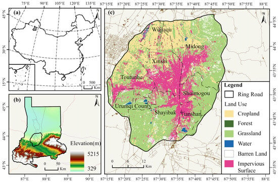
Figure 1. Overview Map of the Study Area. (a) Location of the Urumqi metropolitan area within China. (b) Location of the Third Ring Road within the metropolitan area and its topography. (c) The Third Ring with land use categories.

2.2. Data Source and Preprocessing

Geographical spatial data and remote sensing imagery were used in this study. Due to limitations in data availability, both datasets cover a 10-year period. Data were ultimately obtained at 5-year intervals for 2010, 2015, and 2020. LST represents daytime summer averages (June–September), and only images with less than 10% cloud cover were included. Geographical spatial data were converted to raster format through kernel density analysis in ArcGIS Pro 3.4.2. All datasets were clipped to the study area using a predefined mask. Because blue–green space within urban areas of arid regions is limited in both quantity and spatial scale, a grid resolution of 100 m was selected to balance computational efficiency and spatial detail. To ensure spatial consistency, nighttime light data were resampled to 100 m. The sources of all datasets are listed in Table 2.

Table 2. Data Source Table.

Data Type	Data Name	Website
land use data	China Land Cover Dataset	https://engine-aiearth.aliyun.com/#/ (accessed on 11 May 2025)
LST data	Landsat satellite data inversion	https://www.gscloud.cn/ (accessed on 13 May 2025)
Road data	Openstreetmap	https://download.geofabrik.de/asia/china.html (accessed on 15 May 2025)
	Baidu Maps	https://lbsyun.baidu.com/ (accessed on 15 May 2025)
Population data	Worldpop	https://www.worldpop.org/ (accessed on 17 May 2025)
POI data	Amap	https://lbs.amap.com/ (accessed on 20 May 2025)
	Baidu Maps	https://lbsyun.baidu.com/ (accessed on 21 May 2025)
NTL data	NPP-VIIRS-like NTL Data	https://engine-aiearth.aliyun.com/#/ (accessed on 23 May 2025)

Six land use categories comprise the classification within the study area: cropland, forest, impervious surface, water, grassland, water and bare land. In previous studies, cropland forests, grasslands and water were often classified as blue–green spaces, while impervious and bare land were classified as non-blue–green spaces [9,29]. In dryland oasis cities, grasslands surrounding urban areas are predominantly low-cover grasslands. The mean LST in 2010, 2015, and 2020 were 42.29 °C, 44.35 °C, and 41.77 °C, respectively. These values were higher than the mean LST of impervious surfaces in the same years. Thus, grassland did not provide cooling for the urban area. We therefore classified grassland as non–blue–green space. The technical roadmap is presented as follows (Figure 2):

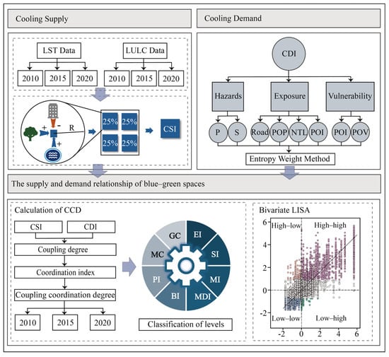
Figure 2. The technical route of the study.

3. Method

3.1. Temperature Grade Division

LST data for the study area were retrieved using the single-window algorithm throughout the summer season (June–September). [30]. The mean value was calculated, and the image data was output on the GEE platform. LST was categorized into 5 grades via the mean standard deviation method. This approach effectively characterizes temperature concentration and fluctuation by combining the mean with varying standard deviation multiples [26]. Table 3 shows the classification basis of LST:

Table 3. The LST level classification criteria.

Classification	Criteria for Classification
Extreme High-Temperature (EHT)	$T>\mu +1.5std$
High-Temperature (HT)	$\mu +0.5std<T\le \mu +1.5std$
Medium Temperature (MT)	$\mu -0.5std\le T<\mu +0.5std$
Low-Temperature (LT)	$\mu -1.5std\le T<\mu -0.5std$
Extreme Low-Temperature (ELT)	$T<\mu -1.5std$

3.2. Construction of Improved Blue–Green Space Cooling Indicators

Researchers have proposed various methods to assess the cooling capacity of blue–green spaces at different spatial scales. At the scale of urban agglomerations and metropolitan areas, calculations focus on representing the overall extent of blue–green space and its combined effects on the thermal environment. As a result, land use-based supply capacity and cold-island supply capacity are often used as core indicators [29,31]. At the city scale, the research objective shifts toward refined management of internal spatial layouts. Methods at this scale further consider spatial associations among blue–green patches and the effects of their configuration [19].

However, most existing studies focus on cities in humid regions. These cities typically feature high vegetation coverage and relatively continuous built-up areas. In contrast, cities in arid regions retain substantial bare land patches within their urban boundaries. These areas form persistent high-temperature zones [32]. Meanwhile, some patches with low vegetation cover do not necessarily act as cooling sources and may even contribute to surface heating [33]. Under these conditions, directly adopting cooling indicators designed for humid-region cities may overestimate the cooling contribution of certain green areas and underestimate the disturbance caused by high-temperature patches to the overall cooling supply. Therefore, it is necessary to refine and extend existing cooling indicators to better capture the thermal characteristics of oasis cities in arid regions.

This study refines the modeling of cooling supply provided by blue–green spaces at the urban scale. Unlike traditional methods that rely only on the temperature difference between blue–green spaces and a target pixel, our approach incorporates all surrounding land use types—including bare soil and other high-temperature patches—into the spatial weighting process. This allows us to capture the combined thermal effects of heterogeneous surfaces. The cooling supply consists of two components. The first is cooling intensity, quantified by the average temperature difference of each land use type relative to the background temperature. The second is cooling extent, represented by a distance-decaying weight that measures the effective influence of surrounding blue–green patches. The product of these two components yields the integrated cooling index, enabling the model to reflect warming disturbances from high-temperature patches. To evaluate the effectiveness of this method, we use Spearman’s rank correlation to test the relationship between the cooling index and LST. The construction of the cooling supply indicators (CSI) includes the following three steps:

(1) Obtain the cooling contributions of each type of land use:

$${CI}_n=T_n-T_{mean}$$

(1)

where ${CI}_n$ is the cooling contribution of land use type $n$, $T_n$ is the average LST of n-type land use. $T_{mean}$ is the average LST within the study area.

(2) For target pixel $i$, accounting for distance-decaying cooling effects from surrounding buffer zone grids, the spatial-weighted contribution of land use type n is calculated:

$${GT}_{ni}=\sum _{j\in B_i}{\displaystyle \frac{{CI}_{nj}}{d_{ij}^e}}$$

(2)

where ${GT}_{ni}$ is the spatial weighted cooling contribution of the i-th pixel to the n-type land use type, $B_i$ is all the pixels within the buffer zone surrounding the i-th pixel. All the land use types within this buffer zone are spatially correlated with the pixel $i$. ${CI}_{nj}$ is the cooling contribution of each type of land use corresponding to pixel $j$ within the buffer zone. $d_{ij}^e$ is the power function of the Euclidean distance between pixels $i$ and $j$, and $e$ = 2 [34,35]. The values of the pixels within the radius of the buffer zone are set to 1 km.

(3) For every analysis grid, determine its corresponding CSI value:

$$CSI=\sum {\displaystyle \frac{G{T}_{ni}{S}_i}{S}}$$

(3)

where $S_i$ is the area of the target pixel $i$, $S$ represents the total area of the analysis grid.

3.3. Establishment of Blue–Green Space Demand Indicators

The cooling demand indicators (CDI) was calculated using the risk assessment framework of the IPCC [36]. Physical and social demand factors were quantified across three dimensions: hazards (Dh), exposure (De), and vulnerability (Dv). The disaster degree represents the cooling demand of physical factors, which is quantified by two secondary indicators: the landscape proportion of high-temperature patches (PLAND) and the complexity of shape (SHAPE). The exposure degree represents the cooling demand of social factors, describing the economic and social activities of the urban population, and is quantified by four secondary indicators: road density (ROAD), population density (POP), urban life service facilities (POI), and night light data (NTL). The vulnerability represents the cooling demand of social factors, describing the geographical distribution of vulnerable groups and their activities, and is quantified by two secondary indicators: vulnerability facility density (POI_V) and vulnerable population density (POP_V).

The PLAND index and SHAPE index can be calculated using the Fragstats 4 software. The ROAD index, POI index, and POI_V index can be obtained by converting point data and line data into density raster maps through the kernel density analysis tool in ArcGIS Pro 3.4.2. The POP_V index is calculated based on the original raster, with different weights assigned to different age groups of vulnerable populations. The weight coefficient distribution assigns values as follows: ages 0 and 80 receive 1, ages 1 and 75 receive 0.8, ages 5 and 70 receive 0.6, ages 10 and 65 receive 0.4, and ages 15 and 60 receive 0.2.

The entropy weight method determines the weighting of each indicator in the Blue–Green Space Cooling Demand Index [37], and then performs a weighted calculation of multiple indicators based on these weights. The computational procedure for the entropy weight method proceeds as follows:

$${x^{\prime }}_{ij}=\frac{x_{ij}-\mathit{min}(x_j)}{\mathit{max}\{x_j\}-\mathit{min}\{x_j\}}\left(i=1,2,\dots ,m\right)\left(1,2,\dots ,n\right)$$

(4)

$$P_{ij}={\displaystyle \frac{{x^{\prime }}_{ij}}{\sum _{i=1}^m{x^{\prime }}_{ij}}}$$

(5)

$$e_j=-{\displaystyle \frac{1}{lnm}}\times \sum _{i=1}^m(P_{ij}\times ln{P}_{ij})$$

(6)

$$w_j={\displaystyle \frac{1-e_j}{\sum _{j=1}^n(1-e_j)}}$$

(7)

$$CDI={\beta }_1{D}_h+{\beta }_2{D}_e+{\beta }_3{D}_v$$

(8)

where $x_{ij}$ is the original value of indicator j in grid i, ${x^{\prime }}_{ij}$ is the standardized value of $x_{ij}$, $P_{ij}$ is the proportion of indicator j in grid i, $e_j$ is the entropy value of indicator $j$, $w_j$ is the weight of indicator j, $D_h$,  $D_e$ and $D_v$ respectively correspond to the indicators of hazards, exposure and vulnerability. ${\beta }_1$,  ${\beta }_2$ and ${\beta }_3$ respectively correspond to the weights of the three indicators calculated using the entropy weight method. To evaluate the effectiveness of this method, we used Pearson correlation test to examine the relationship between demand index and surface temperature.

3.4. Framework for Analyzing the Supply–Demand Relationship of Blue–Green Spaces

3.4.1. Coupling Coordination Degree

Derived from physics’ coupling concept, the coupling coordination degree (CCD) model quantifies interaction intensity and coordinated development levels among multiple systems. This CCD model has been applied in various fields, including the interaction between urbanization and socio-economy, as well as food–energy–water–carbon coupling, etc. [38] The calculation formula is presented below:

$$C=2\sqrt{{\displaystyle \frac{F\left(x\right)\times G\left(y\right)}{{ [F\left(x\right)+G(y\left)\right]}^2}}}$$

(9)

$$T=\alpha F\left(x\right)+\beta G\left(y\right)$$

(10)

where $C$ is coupling degree, representing the intensity of interaction between systems, with a value range of [0, 1], $F\left(x\right)$ and $G\left(y\right)$ are the combined indices of two systems, $T$ is the comprehensive coordination index, where $\alpha$ and $\beta$ are the weight coefficients, and they are usually set as $\alpha$ = $\beta$ = 0.5.

$$D=\sqrt{C\times T}$$

(11)

where $D$ is the Coupling Coordination Index. Drawing on existing literature and data characteristics, this research classifies the Coupling Coordination into 8 distinct tiers: namely extreme discoordination (0 ≤ D ≤ 0.2), severe discoordination (0.2 < D ≤ 0.3), moderate discoordination (0.3 < D ≤ 0.4), mild discoordination (0.4 < D ≤ 0.5), basically discoordinated (0.5 < D ≤ 0.6), primary discoordination (0.6 < D ≤ 0.7), moderate coordination (0.7 ≤ D ≤ 0.8), and good coordination (0.8 < D ≤ 1).

3.4.2. Bivariate Spatial Autocorrelation

Bivariate Spatial Autocorrelation employs spatial statistics to examine dependence patterns and interrelationships between two geographic variables. The method’s core function is to assess covariation levels of variable values within geographical units and reveal spatial agglomeration or discrete trends. The global and local bivariate spatial autocorrelation can be calculated using the GEODA 1.22 software. The calculation formulas are as follows [39]:

$$I_{Global}={\displaystyle \frac{{\sum }_i^m{\sum }_{j=i}^m{w}_{ij}\times (Y_i -\stackrel{-}{Y})(Y_j -\stackrel{-}{Y})}{S^2{\sum }_i^m{\sum }_{j\ne i}^m{w}_{ij}}}$$

(12)

where $I_{Global}$ is the bivariate global spatial autocorrelation value, $Y_i$ and $Y_j$ are the attribute values of spatial units i and j, $n$ is the number of spatial units, $w_{ij}$ is a weight matrix established based on spatial adjacency relationships.

$$I_{Bivariate}={\displaystyle \frac{n{\sum }_{i=1}^n{\sum }_{j=1}^n{\omega }_{ij}(y_i^p-{\stackrel{-}{y}}_p)(y_j^q-{\stackrel{-}{y}}_q)}{\left({\sum }_{i=1}^n{\sum }_{j=1}^n \right)\sum _{i=1}^n(y_i^p-{\stackrel{-}{y}}_p)(y_j^q-{\stackrel{-}{y}}_q)}}$$

(13)

$$I_{lm}^p=z_l^p·\sum _{q=1}^n{W}_{pq}·z_m^q$$

(14)

$$z_l^p={\displaystyle \frac{X_l^p-{\stackrel{-}{X}}_l}{e_l}}$$

(15)

$$z_m^q={\displaystyle \frac{X_m^q-{\stackrel{-}{X}}_m}{e_m}}$$

(16)

where $I_{Bivariate}$ is the bivariate local spatial autocorrelation value; $n$ is the number of spatial units; ${\omega }_{ij}$ is the spatial weight; $y_i^p$ and $y_j^q$ are the attribute values of spatial units in attributes p and q; ${\stackrel{-}{y}}_p$ and ${\stackrel{-}{y}}_q$ are the average values of attributes p and q; $I_{lm}^p$ is the bivariate local spatial autocorrelation index; $X_l^p$ is the attribute value of attribute l of spatial unit p; $X_m^q$ is the attribute value of attribute m of spatial unit q; ${\stackrel{-}{X}}_l$ and ${\stackrel{-}{X}}_m$ are the average values of attributes l and m; $e_l$ and $e_m$ are the variances of attributes l and m.

4. Results

4.1. Spatiotemporal Variations in Land Surface Temperature and Blue–Green Space

4.1.1. Spatiotemporal Variations in Land Surface Temperature

Figure 3 shows that the areas of all temperature categories decrease progressively from the largest to the smallest. In 2010 and 2020, the order remained MT > LT > HT > EHT > ELT. In 2015, the area of high temperature exceeded that of low temperature, while extremely low temperature surpassed extremely high temperature. The combined extremely high- and high-temperature zones accounted for 19.02% in 2010, 21.79% in 2015, and 17.83% in 2020. This proportion increased and then declined, resulting in an overall reduction. Extremely high and high temperatures were mainly distributed northeast and southwest of the built-up area. In 2015, extremely high-temperature zones shifted toward the southwest. Medium-temperature coverage declined from 2010 to 2015 and later increased, showing limited overall variation. Between 2010 and 2015, the spatial center shifted from the central–southern region to the urban core. From 2015 to 2020, the distribution expanded northwestward. The combined extremely low- and low-temperature areas accounted for 18.85%, 19.58%, and 20.02% in 2010, 2015, and 2020, respectively, showing a continuous upward trend. These temperatures were predominantly distributed in the northwest, central, and southeast. The northwest experienced lower temperatures due to the high vegetation density of cropland. In 2010, the central and southwestern regions formed the main medium-temperature zones because of the built-up area. With increased greening in subsequent years, these zones became the primary low-temperature areas in 2015 and 2020. Areas of sparse grassland and bare land surrounding the city formed the high-temperature zones. Overall, the study area exhibited a daytime cold-island pattern.

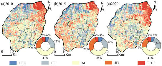
Figure 3. LST classification map, (a) shows the LST classification in 2010, (b) shows the LST classification in 2015, and (c) shows the LST classification in 2020.

4.1.2. Temporal and Spatial Changes in Blue–Green Spaces

As shown in the blue–green space distribution map (Figure 4), non-blue–green spaces account for 70–80% of the study area. Green spaces represent approximately 30%, while blue spaces constitute only 0.7%. From 2010 to 2020, green space coverage declined markedly, decreasing by 11% over the decade. Blue spaces also exhibited a slight downward trend. Blue spaces are primarily located in the outer urban districts and are composed mainly of several large lakes. Green spaces are concentrated in the cropland areas of the northwestern region. The reduction in green space occurred largely along the boundary between urban land and cropland, indicating that urban expansion contributed substantially to green space loss in the study area.

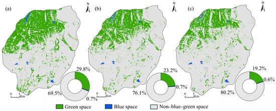
Figure 4. Blue–green space distribution map, (a) shows the blue–green space distribution in 2010, (b) shows the blue–green space distribution in 2015, and (c) shows the blue–green space distribution in 2020.

4.2. Spatiotemporal Changes in the Supply Capacity of Blue–Green Spaces

4.2.1. Evaluation of the Applicability of Supply Indicators

Oasis cities in arid regions exhibit complex thermal conditions in their surrounding areas. As illustrated in the radar chart (Figure 5), water bodies, forests, and cropland show relatively low mean temperatures, whereas grassland, impervious surfaces, and bare land show relatively high mean temperatures. The difference between the lowest and highest mean temperatures exceeds 13 °C. Given these thermal contrasts, it is necessary to evaluate the applicability of the CSI. This study uses the Spearman correlation coefficient for assessment. As shown in Table 4, the p-values for all three years are below 0.01, and the ρ values are approximately −0.5. These results indicate a stable negative relationship between CSI and LST, demonstrating that CSI effectively reflects the cooling capacity of blue–green spaces.

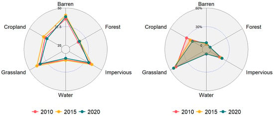
Figure 5. Mean LST of each land use type (left) and their area proportions (right).

Table 4. Correlation Table of CSI and LST.

	Spearman Correlation Coefficient
2010	−0.547 **
2015	−0.552 **
2020	−0.547 **

Note: ** means p < 0.01.

4.2.2. Spatiotemporal Changes in the Supply Capacity of Blue–Green Spaces

Figure 6 illustrates the cooling supply capacity within the three-ring region of Urumqi. Areas with high CSI values (CSI > 4) occupy the smallest proportion, and this proportion shows a slight decline over time. Medium–high CSI areas (2–4) display a pronounced decreasing trend, primarily concentrated in the cropland surrounding the city. In contrast, low CSI areas (0–2) expand significantly, especially within the central and southeastern urban zones. Negative CSI values (CSI < 0) indicate zones that do not provide cooling services and instead contribute to thermal enhancement. These areas account for the largest proportion and exhibit a pattern of initial decline followed by subsequent growth. The notable expansion of low CSI areas and the concurrent reduction in negative CSI areas are associated with increasing vegetation coverage on impervious surfaces. As urban greening intensifies, the mean temperature of impervious surfaces gradually becomes lower than that of adjacent areas, enabling these surfaces to contribute cooling effects. The gradual reduction in medium–high CSI areas is linked to urban expansion, which has increasingly encroached upon surrounding cropland. Greening efforts in newly developed urban zones remain limited, resulting in weaker cooling performance in these areas.

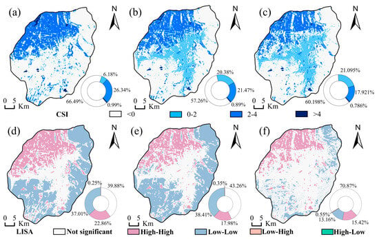
Figure 6. The temporal and spatial distribution map of the cooling supply capacity of blue–green spaces ((a) for 2010, (b) for 2015, (c) for 2020) and the spatial clustering map ((d) for 2010, (e) for 2015, (f) for 2020).

Global Moran’s I values for CSI were 0.857 in 2010, 0.833 in 2015, and 0.811 in 2020, indicating strong spatial autocorrelation throughout the study period. As shown in Figure 6, high–high and low–low clusters form the dominant spatial patterns. High–high clusters are mainly located within the northwestern cropland areas, whereas low–low clusters are concentrated in the eastern and southwestern grassland zones. Areas with insignificant clustering are primarily situated within the central impervious surfaces. High–high clusters gradually decline over time. Low–low clusters first expand and then contract sharply. Insignificant areas increase progressively. These changes can be explained by two factors. First, urban expansion enlarges the extent of insignificant areas while reducing both high–high and low–low clusters. Second, shifts in low–low clusters are influenced by changes in vegetation coverage within adjacent grassland areas.

4.3. Spatiotemporal Changes in the Demand Levels for Blue–Green Spaces

4.3.1. Evaluation of Cooling Demand Indicators

Using the entropy weight method, the weights of the three evaluation criteria were calculated, and Table 5 presents changes in indicator weights across the study period. In all three years, the combined weight of social demand (De and Dv) exceeded that of physical demand (Dh). The ranking of the three criteria remained consistent: De > Dv > Dh. Among all indicators, vulnerable facilities received the highest weight in each year, with values of 18.8%, 17.04%, and 17.67%. These results suggest that the entropy value of the vulnerable facilities indicator is the lowest, reflecting high data dispersion and substantial regional differences in the distribution of vulnerable facilities.

Table 5. Demand indicator weights and correlations.

Criteria	Index	Weight of Indicator (%)			Correlation with LST
		2010	2015	2020	2010	2015	2020
Hazard	PLAND	15.35%	16.51%	15.93%	0.535 **	0.468 **	0.614 **
	SHAPE	14.99%	16.09%	15.58%	0.538 **	0.473 **	0.613 **
Exposure	ROAD	5.32%	5.44%	4.86%	−0.021 **	−0.135 **	−0.126 **
	POI	14.34%	14.63%	14.87%	−0.024 **	−0.117 **	−0.095 **
	POP	11.91%	12.34%	13.31%	−0.043 **	−0.119 **	−0.094 **
	NTL	7.52%	5.76%	4.53%	−0.029 **	−0.104 **	−0.132 **
Vulnerability	POP_V	11.78%	12.19%	13.24%	−0.043 **	−0.12 **	−0.092 **
	POI_V	18.80%	17.04%	17.67%	−0.023 **	−0.097 **	−0.089 **

Note: ** means p < 0.01.

Table 5 also details Pearson correlation coefficients for every indicator within the three criteria against LST. The high-temperature areas and the complexity of the shape of high temperatures reflected by the physical indicators are directly and strongly correlated with the LST. However, the difference from similar studies in cities in eastern China lies in that the social cooling demand of oasis cities in arid areas is significantly not correlated with the LST. However, spatial autocorrelation analysis shows that both the distribution of social demand and areas with high CDI values are concentrated in the urban core areas, such as Shayibake and Tianshan districts (Figure 7). These areas are also characterized by high population density, concentrated economic activities, and dense service facilities, serving as the main urban centers. CDI demonstrates significant spatial clustering (Global Moran’s I = 0.864/0.831/0.871), with high-high clusters aligning with urban socio-economic hotspots. Therefore, the CDI for green–blue spaces can effectively represent the level of cooling demand within the region.

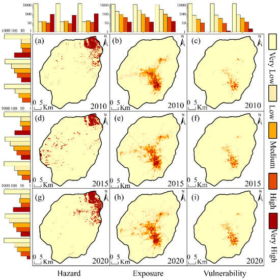
Figure 7. The time-space variation chart of each index for the cooling demand of the blue–green space. ((a) hazard distribution in 2010; (b) exposure distribution in 2010; (c) vulnerability distribution in 2010; (d) hazard distribution in 2015; (e) exposure distribution in 2015; (f) vulnerability distribution in 2015; (g) hazard distribution in 2020; (h) exposure distribution in 2020; (i) vulnerability distribution in 2020.)

4.3.2. Spatial and Temporal Changes in the Level of Cooling Demand

Figure 7 illustrates clear spatial differences between physical and social demands. Physical demands are represented by the Hazard index, which is primarily distributed in the northeastern part of the study area. In 2015, very high physical demand values also appeared slightly in the southwest. These zones correspond mainly to grassland and bare land. The study area is dominated by very low and very high levels, reflecting substantial spatial disparity. Social demands consist of Exposure and Vulnerability and are mainly concentrated within construction areas. Overall changes in the Exposure index are minimal, though low-level zones expand slightly. Most very high Exposure values are located in Shayibak District and Tianshan District in the southern portion of the city. The very high and extremely high Vulnerability levels show an increasing trend and are also concentrated in Shayibak District and Tianshan District.

Figure 8 shows the temporal and spatial changes in the comprehensive index and the degree of concentration of CDI. The high demand caused by physical factors is significantly separated from that caused by social factors. High demand zones in the northeast exhibit concentrations within the 0.2–0.3 range, while those in built-up urban areas diminish progressively outward from the city center. The areas with a demand level of >0.2 in the built-up urban areas mainly concentrate in Shayibak District and Tianshan District, showing a relatively decreasing trend. The area with a demand level of >0.2 in the built-up urban areas is significantly smaller than the area with a demand level of >0.2 in non-land use areas. This indicates that the demand level for cooling in the study area is still dominated by physical factors.

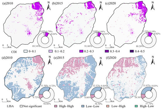
Figure 8. The temporal and spatial distribution map of cooling demand levels in blue–green spaces ((a) for 2010, (b) for 2015, (c) for 2020) and the spatial clustering map ((d) for 2010, (e) for 2015, (f) for 2020).

Global Moran’s I values for CDI were 0.864 in 2010, 0.831 in 2015, and 0.871 in 2020, indicating strong spatial autocorrelation across all three years. Local spatial clustering maps show pronounced high–high (HH) clusters, mainly concentrated in the urban core and in distant suburban areas. A clear low–low clustering pattern is also evident, primarily distributed across cropland zones surrounding the study area. Insignificant clustering is found mainly in suburban and urban–rural fringe areas. The spatial extent of high–high clusters exhibits an overall increasing trend from 2010 to 2020. Mapping results reveal a decline in high–high clustering within the built-up core, accompanied by expansion in the far northwestern suburban sector. This contrasting pattern can be attributed to an increase in the weight of physical factors (from 30.34% to 31.51%), a corresponding decrease in the weight of social factors (from 69.66% to 68.49%), and expansion of high-demand areas driven by physical conditions. Spatial patterns also indicate that high-demand areas associated with social factors have not decreased.

4.4. Coupling Coordination Degree Analysis

Figure 9 and Table 6 indicate that the cooling supply–demand CCD values in the study area remain generally poor. Extremely uncoordinated and severely uncoordinated zones occupy large portions of the region. Extremely uncoordinated zones occur across all land use types and represent the dominant category. Their areal extent continues to increase. Severely uncoordinated zones are located around urban areas and within agricultural land, forming the second most prevalent category. These zones show a declining trend. Moderately uncoordinated areas exhibit minimal change over the three years and are mainly distributed around the urban periphery. Mildly uncoordinated and basically uncoordinated areas are concentrated within the built-up area. Their spatial distribution aligns closely with urban green spaces and parks. Both categories cover relatively small areas and show a decreasing trend. The primary uncoordinated type, which has the highest CCD values, is mainly distributed in the northwestern cropland and accounts for the smallest proportion. The findings indicate that as urban expansion intensifies, the capacity of existing parks and green spaces to meet cooling demand weakens. The northwestern cropland provides substantial cooling supply, yet this potential remains underutilized by the city. Overall, the coordination between cooling supply and cooling demand across the study area remains suboptimal.

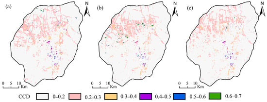
Figure 9. The CCD values of cooling supply–demand levels in blue–green spaces ((a) for 2010, (b) for 2015, (c) for 2020).

Table 6. Coupling and coordination level area proportion.

Level	2010	2015	2020
0–0.2	84.55%	86.11%	87.03%
0.2–0.3	12.86%	11.23%	10.62%
0.3–0.4	1.77%	1.72%	1.77%
0.4–0.5	0.51%	0.39%	0.40%
0.5–0.6	0.23%	0.24%	0.13%
0.6–0.7	0.08%	0.31%	0.05%

4.5. Identification of Supply and Demand Matching

Figure 10 shows the spatial correlation between the CSI and CDI. High-high clustering aligns with the high supply–high demand planning category, whereas low-low clustering matches the low supply–low demand designation. High-low and low-high clusters correspond to imbalanced supply–demand sectors, namely high-supply–low-demand territories and low-supply–high-demand locales. The study has excluded insignificant areas (p value > 0.01), so the four types obtained through the bivariate LISA analysis are all significant clustering types. Figure 10 indicates that statistically non-significant zones concentrate predominantly in urban peripheral suburbs, covering nearly half of the study area. Furthermore, low-supply–low-demand zones cover a substantial portion of the study area, ranging from 17.80% to 21.21%.

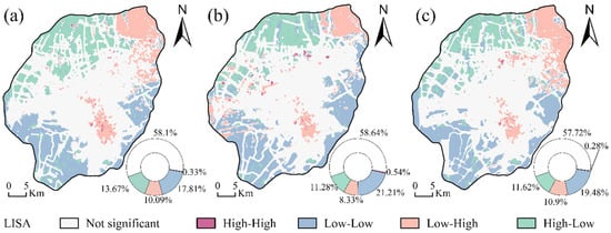
Figure 10. Blue–Green Space Supply–Demand Matching Spatial Distribution Map ((a) for 2010, (b) for 2015, (c) for 2020).

Spatial mismatches between cooling supply and cooling demand represent key areas requiring targeted intervention. High-supply–low-demand zones are concentrated mainly in the northwestern cropland. Their proportions in 2010, 2015, and 2020 were 13.67%, 11.28%, and 11.62%, respectively, showing a downward trend. Low-supply–high-demand zones accounted for 10.09%, 8.33%, and 10.90% in the same years. Although the overall proportion of this category shows no clear trend, its spatial distribution changed considerably. As shown in Figure 10, low-supply–high-demand zones formed two distinct clusters in all three years. These clusters were located in the core urban development areas and in high-temperature zones of the far northeastern suburbs. This pattern indicates that neither socially driven cooling demand nor physically driven cooling demand is well matched by the available cooling supply provided by blue–green spaces. Cooling mismatches driven by social factors decreased from 2010 to 2020, whereas mismatches driven by physical factors increased. The reduction in socially induced mismatches resulted from decreases in their indicator weights. In contrast, the growth of physically induced mismatches was associated with the expansion of high-temperature patches and the increased weight of physical factors. These findings demonstrate that peri-urban high-temperature patches exert a growing influence on overall supply–demand coordination, with their impact intensifying over time.

5. Discussion

5.1. Rethinking the Cool-Island Pattern in Oasis Cities

Analysis of LST patterns from 2010, 2015, and 2020 shows that Urumqi exhibits a distinctive cool-island-like pattern during daytime. Average LST in built-up areas decreased slightly over the decade, while low-temperature zones expanded within the urban core. At the same time, high-temperature patches in surrounding grassland and bare land increased, strengthening the thermal contrast between the city and its periphery.

This cool-island-like pattern should not be interpreted as evidence of ecological optimization within the city. In oasis cities, a decreasing LST in built-up areas does not necessarily indicate improved cooling performance. Instead, it may reflect a widening temperature gap driven by rapid warming in peripheral barren lands. When peripheral heat intensifies, the relative “coolness” of the urban core increases, even if the internal cooling capacity does not strengthen proportionally. Therefore, focusing on creating or enhancing a cold-island effect within built-up areas may be misguided. For arid-region oasis cities, effective thermal regulation depends on regional coordination between cold sources (cropland, vegetation, water bodies) and heat sources (bare land, degraded grassland), rather than the pursuit of a colder urban core alone.

5.2. The Competition of High-Temperature Lesions for Cooling Supply

Based on the IPCC assessment framework, this study established an indicator system to evaluate blue and green space demand. It was found that there are two main components of the cooling and temperature reduction demand for blue–green spaces in Urumqi: the demand caused by physical factors for disaster management and the demand caused by social factors for protection of exposure and vulnerability. Significant spatial disparities exist between the distribution of physical demand and that of social demand. The social demand is distributed in the built-up area, which is a region closely related to humans. While the physical demand is located in the surrounding areas of the city, it indirectly affects human life and health by competing for cooling services from blue and green spaces with the built-up area.

In the special thermal environment pattern distribution of oasis cities in arid regions, this study defines the high-temperature patches (bare land, degraded grassland) as “heat source disturbance areas”. Cropland, as the low-temperature area on the outskirts of the city (cold source), transports cold air through air convection to the city center, forming a “city wind” circulation, thereby alleviating the heat island effect. Numerous high-temperature zones between cropland and urban land reduce the LST contrast between cropland and the urban core, diminishing cold air transport capacity. [40]. The high-temperature patches weaken the function of the suburbs as a cold source, reducing the amount of cold air transported to the city. At the same time, the aggregation area of high-temperature patches on the northwest side not only absorbs the cooling supply from impervious surface but also absorbs the cooling supply from cropland. This causes dual interference to the cooling mechanism of cropland-to-city.

5.3. Planning Suggestions

The regulation of the thermal environment in arid areas should be adapted to local conditions [41]. This study shows a clear spatial pattern in the core built-up area of Urumqi, characterized by insufficient cooling-source supply and highly concentrated social demand. Although the mean LST in the built-up area has declined, the amount, scale, and connectivity of existing blue–green spaces remain inadequate for cooling densely populated zones and clusters of urban services. Therefore, strengthening blue–green infrastructure within the built-up area should be treated as a priority. Key actions include adding micro-green spaces and pocket parks at the block scale, improving the morphological quality and structural complexity of existing green spaces, and enhancing the continuity and shading performance of street trees and roadside vegetation. Green roofs, sunken green spaces, and rain gardens should also be promoted in new developments as effective evapotranspiration-based nature-based solutions. By increasing the internal cooling capacity of the urban core, the city can reduce its reliance on temperature-gradient-driven “passive cool island effects” from the urban periphery and achieve substantial improvements in its internal thermal environment.

The analysis identifies cropland in the northwestern part of Urumqi as the area with the highest cooling-source supply capacity (high CSI). This cropland serves as a major regional cooling source for the city. However, extensive high-temperature patches—mainly bare land and degraded grassland—form belt-like or clustered patterns around the urban boundary. These patches disrupt the movement of cool air from the suburbs to the city center and weaken the cooling support that peripheral sources can provide to the built-up area. To address this issue, continuous ventilation and cool-air corridors connecting regional cooling sources to the built-up area should be developed at the regional scale. Priority measures include protecting cropland, restoring vegetation along cropland edges, and rehabilitating wetlands to maintain the integrity of the northwestern cooling-source area. Degraded grasslands and bare surfaces located along cool-air pathways should undergo vegetation reconstruction and surface temperature control treatments to reduce their blocking effects. Large-scale impervious construction should be avoided at the urban fringe to keep the corridors open and permeable. By restoring the continuity of suburban cooling sources and enhancing their capacity to deliver cool air, cities can fundamentally alleviate the current mismatch between high supply areas and high-demand zones.

Unlike cities such as Phoenix, where cooling strategies focus on regulating the urban microclimate through internal water bodies and park systems [42], Urumqi faces a different challenge. Its primary cooling sources and areas of cooling demand are spatially mismatched. Continuous regional cooling corridors are therefore essential. Urumqi’s approach is characterized by a regional-scale perspective rather than an intra-urban one. This strategy offers a new pathway for mitigating heat stress in other arid-region cities with similar conditions.

5.4. Limitations and Future Perspectives

The precision of land use classification strongly influences this study’s outcomes. The number of land use products used in this paper is insufficient for the detailed identification of blue–green spaces within the city. This approach solely detects major urban parks, overlooking roadside protective greenery and the green areas associated with residential and industrial zones, consequently causing an underestimation of the city’s cooling provision services. In the future, it is possible to try using Sentinel data and machine learning and deep learning algorithms to improve the accuracy of land use classification. In addition, due to the lack of independent external observations, CDI and CSI based area proportions should be interpreted relatively rather than as precise absolute values.

This study infers urban cooling mechanisms and the role of blue–green spaces mainly from the spatial pattern of LST, not from direct observations of surface energy balance components. No measurements were collected for sensible heat flux, latent heat flux, albedo, evapotranspiration, or atmospheric circulation. The cooling processes discussed—such as blocked cold-air corridors and a weakened influence of cold sources—are therefore offered as plausible spatial interpretations. They are not confirmed physical mechanisms. Future work that incorporates in situ observations or remote sensing inversions of energy balance terms will allow clearer testing and quantification of these processes.

This study focuses on Urumqi, an oasis city in an arid region. Land use and the thermal environment around the city are complex. To our knowledge, it is the first to identify a decoupling between the physical and social demand for urban cooling. It also reveals a supply–demand mismatch in their sources. Future research should use multidisciplinary coupled models to analyze coordinated cooling regulation across the city and its surrounding areas in greater detail [43].

6. Conclusions

This study quantified the spatial relationship between cooling supply and cooling demand in Urumqi, an oasis city in an arid region, and identified several defining characteristics of its urban thermal environment.

First, cooling supply is dominated by strong suburban cold sources, particularly the northwestern cropland, while the cooling contribution of urban blue–green spaces remains limited. Second, cooling demand displays a clear dual-core pattern: physical demand is concentrated in peripheral high-temperature zones, whereas social demand is clustered in the urban core. Third, the coordination between supply and demand is extremely weak, with the study area exhibiting widespread mismatches. The primary constraint arises from the spatial separation between suburban cold sources and high-demand urban areas, a condition further exacerbated by the blocking effect of surrounding high-temperature patches.

These findings suggest that improving cooling efficiency in arid-region cities requires regional-scale interventions rather than localized greening alone. In addition to strengthening blue–green infrastructure within the city, reducing peripheral high-temperature zones is essential for restoring the cold–hot gradient and establishing continuous cold-source corridors that link cropland cold sources with high-demand urban sectors. Such strategies offer an effective pathway for enhancing thermal resilience, ecological security, and public health in arid-region cities.

References

- Wang, S.; Zhan, W.; Zhou, B.; Tong, S.; Chakraborty, T.C.; Wang, Z.; Huang, K.; Du, H.; Middel, A.; Li, J.; et al. Dual Impact of Global Urban Overheating on Mortality. Nat. Clim. Change 2025, 15, 497–504. [Google Scholar] [CrossRef]
- Zhu, D.; Ooka, R. WRF-Based Scenario Experiment Research on Urban Heat Island: A Review. Urban Clim. 2023, 49, 101512. [Google Scholar] [CrossRef]
- Zhang, P.; Zhang, J.; Liu, Z.; Liu, Y.; Chen, Z. Relationship between Land Surface Temperature and Air Quality in Urban and Suburban Areas: Dynamic Changes and Interaction Effects. Sustain. Cities Soc. 2025, 118, 106043. [Google Scholar] [CrossRef]
- Liu, Z.; Zhang, S. Exploring the Relationship between Urban Green Development and Heat Island Effect within the Yangtze River Delta Urban Agglomeration. Sustain. Cities Soc. 2025, 121, 106204. [Google Scholar] [CrossRef]
- Yu, Z.; Yang, G.; Zuo, S.; Jørgensen, G.; Koga, M.; Vejre, H. Critical Review on the Cooling Effect of Urban Blue-Green Space: A Threshold-Size Perspective. Urban For. Urban Green. 2020, 49, 126630. [Google Scholar] [CrossRef]
- Das, M.; Das, A.; Saha, P.; Paul, S. Impact of Spatial Configuration of Urban Blue Spaces in Mitigating Temperature during Summer: A Remote Sensing and Field-Based Observation. Sustain. Cities Soc. 2025, 127, 106418. [Google Scholar] [CrossRef]
- Yang, L.; Liu, X.; Qian, F. Research on Water Thermal Effect on Surrounding Environment in Summer. Energy Build. 2020, 207, 109613. [Google Scholar] [CrossRef]
- Liu, Q.; Dong, Q.; Zhang, L.; Sun, C. Summer Cooling Island Effects of Blue-Green Spaces in Severe Cold Regions: A Case Study of Harbin, China. Build. Environ. 2024, 257, 111539. [Google Scholar] [CrossRef]
- Gao, H.; Chen, Y.; Li, K.; Gao, S. People’s Exposure to Blue-Green Spaces Decreased but Inequality Increased during 2001–2020 across Major Chinese Cities. Ecol. Indic. 2024, 166, 112571. [Google Scholar] [CrossRef]
- Tache, A.-V.; Popescu, O.-C.; Petrișor, A.-I. Planning Blue–Green Infrastructure for Facing Climate Change: The Case Study of Bucharest and Its Metropolitan Area. Urban Sci. 2024, 8, 250. [Google Scholar] [CrossRef]
- Wong, N.H.; Yu, C. Study of Green Areas and Urban Heat Island in a Tropical City. Habitat Int. 2005, 29, 547–558. [Google Scholar] [CrossRef]
- Hamada, S.; Ohta, T. Seasonal Variations in the Cooling Effect of Urban Green Areas on Surrounding Urban Areas. Urban For. Urban Green. 2010, 9, 15–24. [Google Scholar] [CrossRef]
- Yu, Z.; Guo, X.; Jørgensen, G.; Vejre, H. How Can Urban Green Spaces Be Planned for Climate Adaptation in Subtropical Cities? Ecol. Indic. 2017, 82, 152–162. [Google Scholar] [CrossRef]
- Yang, G.; Yu, Z.; Jørgensen, G.; Vejre, H. How Can Urban Blue-Green Space Be Planned for Climate Adaption in High-Latitude Cities? A Seasonal Perspective. Sustain. Cities Soc. 2020, 53, 101932. [Google Scholar] [CrossRef]
- Liu, Y.; Li, G. Inequities in Thermal Comfort and Urban Blue-Green Spaces Cooling: An Explainable Machine Learning Study across Residents of Different Socioeconomic Statuses in Hangzhou, China. Sustain. Cities Soc. 2025, 127, 106427. [Google Scholar] [CrossRef]
- He, M.; Yuan, C.; Zhang, X.; Wang, P.; Yao, C. Impacts of Green-Blue-Grey Infrastructures on High-Density Urban Thermal Environment at Multiple Spatial Scales: A Case Study in Wuhan. Urban Clim. 2023, 52, 101714. [Google Scholar] [CrossRef]
- Zhou, L.; Hu, F.; Wang, B.; Wei, C.; Sun, D.; Wang, S. Relationship between Urban Landscape Structure and Land Surface Temperature: Spatial Hierarchy and Interaction Effects. Sustain. Cities Soc. 2022, 80, 103795. [Google Scholar] [CrossRef]
- Fricke, L.; Legg, R.; Kabisch, N. Impact of Blue Spaces on the Urban Microclimate in Different Climate Zones, Daytimes and Seasons—A Systematic Review. Urban For. Urban Green. 2024, 101, 128528. [Google Scholar] [CrossRef]
- Wang, Y.; Ouyang, W.; Zhang, J. Matching Supply and Demand of Cooling Service Provided by Urban Green and Blue Space. Urban For. Urban Green. 2024, 96, 128338. [Google Scholar] [CrossRef]
- Pritipadmaja; Garg, R.D.; Sharma, A.K. Assessing the Cooling Effect of Blue-Green Spaces: Implications for Urban Heat Island Mitigation. Water 2023, 15, 2983. [Google Scholar] [CrossRef]
- Zhang, Y.; Ge, J.; Bai, X.; Wang, S. Blue-Green Space Seasonal Influence on Land Surface Temperatures across Different Urban Functional Zones: Integrating Random Forest and Geographically Weighted Regression. J. Environ. Manag. 2025, 374, 123975. [Google Scholar] [CrossRef] [PubMed]
- Zhou, W.; Yu, W.; Wu, T. An Alternative Method of Developing Landscape Strategies for Urban Cooling: A Threshold-Based Perspective. Landsc. Urban Plan. 2022, 225, 104449. [Google Scholar] [CrossRef]
- Wang, C.; Liu, X.; Wu, J.; Qiao, W.; Liu, Y. Planning a Water-Constrained Ecological Restoration Pattern to Enhance Sustainable Landscape Management in Drylands. J. Environ. Manag. 2023, 335, 117514. [Google Scholar] [CrossRef] [PubMed]
- Lu, X.; Zou, M.; Gan, G.; Kang, S. Excessive Irrigation-Driven Greening Has Triggered Water Shortages and Compromised Sustainability. Agric. Water Manag. 2025, 311, 109405. [Google Scholar] [CrossRef]
- Zhang, P.; Dong, Y.; Ren, Z.; Wang, G.; Guo, Y.; Wang, C.; Ma, Z. Rapid Urbanization and Meteorological Changes Are Reshaping the Urban Vegetation Pattern in Urban Core Area: A National 315-City Study in China. Sci. Total Environ. 2023, 904, 167269. [Google Scholar] [CrossRef]
- Liang, H.; Kasimu, A.; Zhang, X.; Zhao, Y.; Reheman, R. Spatio-Temporal Change and Influencing Factors of Land Surface Temperature in Oasis Urban Agglomeration in Arid Region: A Case Study in the Urban Agglomeration on the Northern Slope of Tianshan Mountains. Acta Ecol. Sin. 2023, 43, 3650–3664. [Google Scholar] [CrossRef]
- Ma, Y.-J.; Xu, Y.; Yang, T.; Xiao, H.-W.; Xiao, H.-Y. Measurement Report: Characteristics of Nitrogen-Containing Organics in PM2.5 in Ürümqi, Northwestern China—Differential Impacts of Combustion of Fresh and Aged Biomass Materials. Atmos. Chem. Phys. 2024, 24, 4331–4346. [Google Scholar] [CrossRef]
- Abulimiti, A.; Liu, Y.; Tang, J.; Mamtimin, A.; Yao, J.; Zeng, Y.; Abulikemu, A. Urbanization Effect on Regional Thermal Environment and Its Mechanisms in Arid Zone Cities: A Case Study of Urumqi. Remote Sens. 2024, 16, 2939. [Google Scholar] [CrossRef]
- Fang, Y.; Zhao, L. Exploring the Supply-Demand Match and Drivers of Blue-Green Spaces Cooling in Wuhan Metropolis. Urban Clim. 2024, 58, 102194. [Google Scholar] [CrossRef]
- Deng, Y.; Jiang, W.; Ling, Z.; Liu, L.; Sun, S. Revealing the Driving Factors of Urban Wetland Park Cooling Effects Using Random Forest Regression and SHAP Algorithm. Sustain. Cities Soc. 2025, 120, 106151. [Google Scholar] [CrossRef]
- Shen, Z.-J.; Zhang, B.-H.; Xin, R.-H.; Liu, J.-Y. Examining Supply and Demand of Cooling Effect of Blue and Green Spaces in Mitigating Urban Heat Island Effects: A Case Study of the Fujian Delta Urban Agglomeration (FDUA), China. Ecol. Indic. 2022, 142, 109187. [Google Scholar] [CrossRef]
- Kasimu, A.; Maitiniyazi, M. Study on Land Surface Characteristics and Its Relationship with Land Surface Thermal Environment of Typical City in Arid Region. Ecol. Environ. Sci. 2015, 24, 1865–1871. [Google Scholar] [CrossRef]
- Cheng, Y.; An, Q.; Liu, L.; Zhang, Y.; Li, H.; Liu, X.; Huang, G. Latitudinal and Seasonal Asymmetry in Land Surface Temperature Responses to Vegetation Greening Across China. Earth’s Future 2025, 13, e2025EF006385. [Google Scholar] [CrossRef]
- Du, K.; Fan, J.; Chen, X. Study on the Cooling Effect of Parks in the Central Urban Area of Urumqi. Sci. Surv. Mapp. 2024, 49, 168–176. [Google Scholar] [CrossRef]
- Wang, Y.; Zhan, Q.; Ouyang, W. How to Quantify the Relationship between Spatial Distribution of Urban Waterbodies and Land Surface Temperature? Sci. Total Environ. 2019, 671, 1–9. [Google Scholar] [CrossRef]
- IPCC. Climate Change 2022—Impacts, Adaptation and Vulnerability: Working Group II Contribution to the Sixth Assessment Report of the Intergovernmental Panel on Climate Change, 1st ed.; Cambridge University Press: Cambridge, UK, 2023; ISBN 978-1-009-32584-4. [Google Scholar]
- Guo, F.; Zheng, R.; Zhao, J.; Zhang, H.; Dong, J. Framework of Street Grid-Based Urban Heat Vulnerability Assessment: Integrating Entropy Weight Method and BPNN Model. Urban Clim. 2024, 56, 102067. [Google Scholar] [CrossRef]
- Fang, Y.; Meng, F.; Luo, M.; Sa, C.; Bao, Y.; Lei, J. Coupling Coordination Framework for Assessing Balanced Development Between Potential Ecosystem Services and Human Activities. Earth’s Future 2025, 13, e2025EF006243. [Google Scholar] [CrossRef]
- Yan, G.; Wang, S. Coexistence and Transformation from Urban Industrial Land to Green Space in Decentralization of Megacities: A Case Study of Daxing District, Beijing, China. Ecol. Indic. 2023, 156, 111120. [Google Scholar] [CrossRef]
- Zhang, X.; Kasimu, A.; Liang, H.; Wei, B.; Aizizi, Y.; Zhao, Y.; Reheman, R. Construction of Urban Thermal Environment Network Based on Land Surface Temperature Downscaling and Local Climate Zones. Remote Sens. 2023, 15, 1129. [Google Scholar] [CrossRef]
- Kasimu, A.; Zhang, X.; Liang, H. The Spatial Relationship between Seasonal Surface Temperature Andlandscape Pattern of the Urban Agglomeration on the Northern Slope of the Tianshan Mountains. Geogr. Res. 2024, 43, 1267–1287. [Google Scholar]
- Jenerette, G.D.; Harlan, S.L.; Buyantuev, A.; Stefanov, W.L.; Declet-Barreto, J.; Ruddell, B.L.; Myint, S.W.; Kaplan, S.; Li, X. Micro-Scale Urban Surface Temperatures Are Related to Land-Cover Features and Residential Heat Related Health Impacts in Phoenix, AZ USA. Landsc. Ecol. 2016, 31, 745–760. [Google Scholar] [CrossRef]
- Paton, E.; Nardi, M.; Churkina, G.; Hoffmann, K.; Joseph, B.; Kluge, B.; Salim, M.; Schubert, S.; Tams, L. Merits, Limits and Preposition of Coupling Modelling Tools for Blue-Green Elements to Enhance the Design of Future Climate-Resilient Cities. Environ. Res. Lett. 2025, 20, 043002. [Google Scholar] [CrossRef]
Disclaimer/Publisher’s Note: The statements, opinions and data contained in all publications are solely those of the individual author(s) and contributor(s) and not of MDPI and/or the editor(s). MDPI and/or the editor(s) disclaim responsibility for any injury to people or property resulting from any ideas, methods, instructions or products referred to in the content. |
© 2025 by the authors. Licensee MDPI, Basel, Switzerland. This article is an open access article distributed under the terms and conditions of the Creative Commons Attribution (CC BY) license.