Hyperspectral Signatures for Detecting the Concrete Hydration Process Using Neural Networks

Abstract

The curing process of a concrete sample has a significant influence on hydration and its strength. This means that inadequate curing conditions lead to a loss of concrete quality and negative consequences in structural engineering. In addition, different state-of-the-art (SOTA) curing surface treatments and hydration periods have a significant effect on durability. This paper introduces an innovative non-destructive method to detect the development of the hydration process under different treatment conditions. Hyperspectral imaging is a non-contact measurement technique that provides detailed information on hydration characteristics within an electromagnetic wavelength range. A comparative laboratory measurement was conducted on twelve concrete samples, subjected to three curing treatments and four curing surface treatments, over a hydration period from the 1st to the 56th day. Additionally, artificial neural networks and convolutional neural networks have achieved classification accuracies of 67.8% (hydration time), 83.3% (curing regime), and 87.6% (surface type), demonstrating the feasibility of using neural networks for hydration monitoring. In this study, the results revealed differences in near-infrared spectral signatures, representing the type of curing treatment, curing surface, and hydration time of the concrete. The dataset was classified and analyzed using neural networks. For each hydration treatment, three different models were developed to achieve better prediction performance for hyperspectral imaging analysis. This method demonstrated a high level of reliability in investigating curing surface treatments, curing treatments, and hydration time. A recommended method for using hyperspectral imaging to evaluate the cured quality of concrete will be developed in future research.

1. Introduction

As a fundamental industry in national development, infrastructure significantly affects all aspects of daily life and promotes the advancement of human civilization. Conversely, human needs and social productivity drive the advancement of infrastructure and transportation development. Recently, various fields, including science and technology, culture, politics, economy, and daily life, have profoundly influenced infrastructure development. With the continuous progress in civil engineering, almost all infrastructure naturally deteriorates over time.

The concrete industry is an essential raw material sector for national development, production, and daily life [1]. It is one of the most important building materials in modern times. Contemporary concrete offers enhanced performance, including low water content, superior tensile properties, and excellent durability under various complex environmental conditions. These properties contribute to improved structural performance, increased stiffness, reduced deformation, and better seismic resistance. However, as concrete ages under long-term natural conditions, it may no longer meet traffic support requirements, leading to a gradually shortened lifespan.

The production of concrete primarily involves three main processes: hydration, curing, and hardening [2]. During hydration, a chemical reaction forms cement stone, bonding with composite materials to create concrete. Proper hydration, with adequate moisture, is crucial for achieving the desired strength. Insufficient hydration can lead to drying effects, increasing the formation of capillary pores [3]. As a result, the structure of the peripheral and surrounding concrete remains porous, reducing surface strength and leading to the development of chemical shrinkage cracks, among other defects [4]. Furthermore, monitoring the quality of curing concrete components under non-destructive conditions presents a significant challenge due to the material’s characteristics.

Hydration detection technology offers a convenient, non-contact, and non-destructive measurement method with minimal sample requirements. Additionally, spectrometers collect spectral reflectance and emissivity data across hundreds of spectral wavelengths [5]. Research on the hyperspectral properties of concrete plays a crucial role in improving production processes and advancing the application of concrete in complex building systems [6].

Based on these methodologies and concrete research, a proposed neural network analysis has been applied to study concrete properties. A large hyperspectral dataset will be collected and analyzed using artificial neural networks. This approach introduces a concept in which cascade neurons work together to process and transmit information [7]. These networks are specifically designed to simulate human logic, knowledge acquisition, and problem-solving mechanisms that resemble the reasoning processes of the human brain, as illustrated in Figure 1.

The first layer in artificial neural networks is called the input layer, which is responsible only for receiving input data and mapping it to an array of related features without an activation function. Subsequently, all intermediate layers in artificial neural networks are known as hidden layers, which extract more complex features through the calculation of ReLU activation functions. However, if the network contains too many neurons in the hidden layers, it may cause overfitting, where the network simply memorizes input patterns rather than learning meaningful representations.

Finally, the last layer is the output layer, where the number of neurons corresponds to the number of label categories and is typically processed using the Softmax activation function. This allows for object categorization and classification in artificial neural networks [8]. However, another method, the convolutional neural network (CNN), was implemented to recognize a large number of image features and datasets, as shown in Figure 2.

A CNN consists of convolutional layers, max-pooling layers, fully connected layers, and a classification layer. The first convolutional layer typically captures low-level features such as gradient orientation, edges, and colors. The design adapts to higher-level features by adding additional layers, enabling the network to fully understand image features from the dataset. As shown in Figure 3, for example, a 5 × 5 × 5 image is transformed into a 7 × 7 × 1 image and then multiplied by a 3 × 3 × 1 kernel over each channel. Through this padding method and the convolution kernel mechanism, the main features of the image can be extracted [9].

Next, a max-pooling layer is added to perform a common operation in convolutional neural networks, mimicking the human visual system for dimensionality reduction. This helps reduce the feature size of the output from the convolutional layer and prevents overfitting. Furthermore, the fully connected layer serves as the classifier in the neural network, mapping the extracted features to sample labels. It also performs the weighted sum of the previously designed features, as shown in Figure 4 [9].

For classification, the core operation of the fully connected layer is matrix multiplication, which is essentially a linear transformation of one feature space into another.

Based on the above theory, a graphical illustration of the 1D CNN applied to hyperspectral reflectance processing is shown in Figure 5. A hyperspectral vector is fed into the input layer and then passes through multiple convolutional and pooling layers for feature extraction. The kernel size is a hyper-parameter related to the vector data. In this sense, it helps optimize computational complexity [10].

Recent works have successfully applied neural networks to hyperspectral image (HSI) data for infrastructure monitoring. Zhang et al. used CNNs to detect asphalt defects using HSI data, while Lee et al. demonstrated the feasibility of field hydration monitoring using portable spectral sensors and deep learning [11,12].

Figure 4. Fully connected layer process, extracted from [13].

Figure 4. Fully connected layer process, extracted from [13].

Figure 5. Classification process of reflectance transformation in neural network.

Figure 5. Classification process of reflectance transformation in neural network.

2. Methodology

2.1. Concrete Sample Preparation and Curing Regimes

Twelve concrete samples were fabricated with standardized dimensions (50 cm × 50 cm × 10 cm) using Austrian concrete type B5 (C30/37) with a water-to-cement ratio (w/c) of 0.48. Each specimen was subjected to one of three curing conditions, defined as NB1 (20 °C, 60% RH, with foil), NB2 (20 °C, 60% RH, without foil), and NB3 (30 °C, 40% RH, without foil). These regimes simulate varying practical field curing conditions, ranging from ideal (NB1) to thermally stressed (NB3). Foil was used in NB1 to simulate protective curing membranes, while NB3 aimed to reflect poor hydration conditions due to elevated temperature and reduced humidity.

Each surface was further treated to simulate real-world variability in finish and porosity, producing four surface textures per sample: none (smooth), wave (rippled), sand (roughened), and hole (porous) [14]. These treatments represent diverse surface conditions that influence reflectance behavior and moisture evaporation.

Table 1. Material properties of concrete sample.

Austrian Concrete Type	B5
Strength class	C30/37
Cement: CEM/A-M(S-L)42.5N	329 kg/m3
Water	170 kg/m3
w/c ratio	0.48
Stone
Round gravel 16/32 RK	451 kg/m3
Round gravel 8/16 RK	289 kg/m3
Round gravel 4/8 RK	307 kg/m3
Sand 0/4 RK	761 kg/m3
Aggregates	40 kg/m3
Air content (fresh concrete)	2.5–3.6%
Density (fresh concrete)	2383–2442 kg/m3
Fresh concrete temperature	21.8–23.3 °C

summarizes the concrete material properties.

As indicated in

Table 2. Treatment conditions in the curing process.

	Curing Condition
	Storage	Temperature	Humidity	w/c	Surface Treatment
NB1	With foil	20 °C	60%	0.48	Hole, None, Sand, Wave
NB2	Without foil	20 °C	60%	0.48	Hole, None, Sand, Wave
NB3	Without foil	30 °C	40%	0.48	Hole, None, Sand, Wave

, the curing conditions followed environmental classifications NB1, NB2, and NB3 over the first 7-day curing period, as shown in Figure 6.

The selection of the four surface treatments—hole, none, sand, wave—was intended to simulate a range of practical surface textures that may arise from different curing practices or finishing techniques. These surfaces represent smooth, rippled, roughened, and porous textures, respectively, which can affect surface water retention and evaporation rates. Since surface texture alters light scattering and reflectance in HSIs, including these variants enables us to evaluate how real-world surface finishes might impact hydration monitoring accuracy.

After the 7-day curing treatment, the hydration process of each concrete sample was monitored through daily measurements for the first 21 days and weekly measurements from the 21st to the 56th hydration day. Concrete samples with none, wave, sand, and hole surface treatments under NB1, NB2, and NB3 conditions are shown in Figure 7. A total of twelve concrete samples were used for further hydration process research.

Special care was taken to maintain consistent illumination using four symmetrically placed halogen lamps within a semi-enclosed imaging booth. The same lighting setup was used for all samples and curing conditions. Slight visual inconsistencies in Figure 7 are due to natural surface reflectance differences and the camera angle, not changes in lighting configuration. All images were corrected using standardized white and dark reference calibration before reflectance computation.

The complete experimental setup for HSIs is illustrated in Figure 8. The concrete sample surfaces were scanned line-by-line using a push-broom imaging method under halogen illumination. The imaging samples were further processed step by step on different surfaces using a moving semi-enclosed table. Four halogen lamps were installed in the top corners of the semi-enclosed table to provide symmetrical lighting and eliminate the influence of visible light, ensuring optimal conditions for HSIs [15].

For dark reference calibration, the hyperspectral camera was enclosed in a black-lined imaging chamber and directed toward a non-reflective surface fully covered to eliminate ambient light. This method approximates a zero-reflectance (100% absorbance) baseline and ensures consistent two-point calibration. This setup minimized bias due to ambient interference.

Furthermore, nine HSIs were taken for each concrete sample at a distance of 45 cm using the NIR hyperspectral camera. The measurement dataset was processed to analyze the main absorption features at different hydration times [4]. Due to the large surface area of the twelve concrete samples, each surface was divided into nine sections. The detailed process of the experimental setup and data acquisition is further explained in Figure 9.

2.2. Hyperspectral Imaging and Data Acquisition

All samples were scanned using a SPECIM IQ VNIR hyperspectral camera (400–1000 nm, 204 spectral bands, CMOS sensor, SPECIM, FI-90590 Oulu, Finland) under standardized halogen illumination in a semi-enclosed black imaging booth. The samples were imaged using a push-broom scanning method at a 45 cm distance. Each surface was divided into 9 equal segments, and hyperspectral data were collected at 5 hydration ages: 1, 7, 14, 28, and 56 days post-casting. Each region produced approximately 1000 spectral signatures per scan, yielding a total of 12 samples × 9 segments × 5 hydration stages × 1000 spectra = 540,000 spectral vectors.

2.3. Spectral Preprocessing

The raw hyperspectral cubes were denoised using a neighborhood-based algorithm implemented in MATLAB 2018b. Wavelengths outside the reliable range (392–600 nm and 1003–1050 nm) were excluded due to sensor noise and a low signal-to-noise ratio. The final reflectance data spanned 600–1003 nm across 204 wavelengths.

Reflectance values were normalized and analyzed using PLS Toolbox, Eigenvector Research Inc., WA 98831 Manson, USA (Eigenvector Research [16]) to track hydration trends. Emphasis was placed on water-sensitive bands (680 nm and 800–1000 nm), corresponding to known absorption features of free and chemically bound water.

2.4. Dataset Construction and Labeling

Three classification tasks were defined:

• Hydration time (5 classes: days 1, 7, 14, 28, 56);
• Curing regime (3 classes: NB1, NB2, NB3);
• Surface type (4 classes: none, wave, sand, hole).

Each spectral vector was labelled accordingly, and RGB image snapshots (960 × 1280 pixels) were also extracted for surface classification.

Table 3. Components of the experimental setup for the concrete hydration process.

SPECIM IQ camera (hyperspectral camera—VNIR 400–1000 nm (CMOS) with a spectral resolution of FWHM 7 nm, 204 spectral bands, 100 measurements, and one SD card and battery; rescaled to 960 × 1280 pixels under halogen illumination)

50 × 50 × 50 cm semi-enclosed black table

Four stable diffused lights generated by four 9 V halogen bulbs

220 V voltage power 2 × 9 V voltage converter

MATLAB R2018b

MATLAB PLS toolbox

PyCharm CE Version 2023.1

summarizes the components of the spectral processing setup.

2.5. Neural Network Models

2.5.1. 1D Convolutional Neural Network (CNN) for Hydration Time

A 1D CNN was used to classify hydration age from spectral vectors. The architecture included four convolutional layers (kernel size = 3), batch normalization, ReLU activation, and two fully connected layers, followed by Softmax classification. The input dimension was 1 × 204 (spectral vector). The model was trained using the Adam optimizer (learning rate = 0.00023, batch size = 256, epochs = 1000). Early stopping and learning rate decay were applied to avoid overfitting.

2.5.2. Artificial Neural Network (ANN) for Curing Regime

Curing treatment classification was performed using a four-layer fully connected ANN, optimized for low spectral variability. Each input vector (1 × 204) passed through ReLU-activated dense layers. The model was trained for 150 epochs using Adam optimization (learning rate = 0.0001, batch size = 256). This architecture provided a computationally efficient alternative to CNNs with minimal performance loss.

2.5.3. Two-Dimensional CNN for Surface Classification

Surface classification was conducted using RGB images and a 2D CNN consisting of four convolutional layers, max pooling, a fully connected layer, and a Softmax output. This model exploited spatial texture differences among the four surface types. Images were resized and augmented during training. The model was trained with 100 epochs (Adam optimizer, learning rate = 0.001, batch size = 24).

2.6. Evaluation Metrics

Each model was evaluated using accuracy, precision, recall, and F1-score. Class-wise metrics were computed using confusion matrices. Confidence intervals (95%) were calculated through bootstrapping. Results are presented in Section 3 and summarized in

Table 4. Classification metrics for CNN and ANN models across three tasks.

Classification Task	Accuracy %	Precision %	Recall %	F1-Score %	95% CF-Interval
Hydration Time CNN	67.8	66.4	67.1	66.7	[65.2, 70.3]
Curing Treatment ANN	83.3	82.7	83.1	82.9	[81.5, 85.6]
Surface Type CNN	87.6	87.2	87.4	87.3	[85.9, 89.2]

.

3. Result and Discussion

3.1. Result After Concrete Data Analysis

Based on the above experiment and theoretical methods, all results of the analysis and prediction modelling with neural network algorithms for hyperspectral features are demonstrated in the following figures: Figure 10, Figure 11, Figure 12 and Figure 13, which differ in the properties of their spectral signatures.

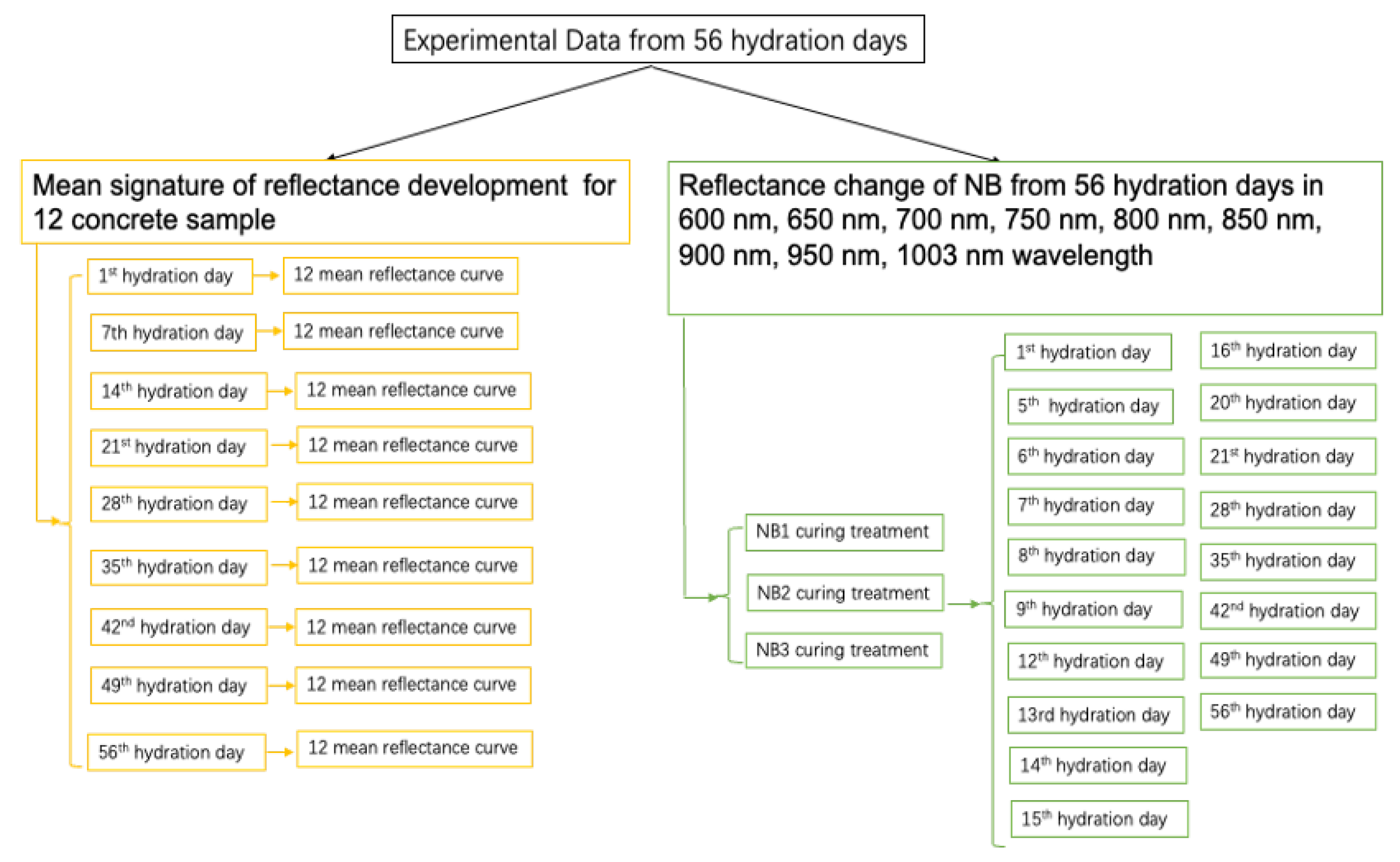
Although HSIs contain hundreds of data points per line scan, we selected 12 spectral signatures per surface region to ensure computational efficiency and maintain a balanced dataset across the entire image matrix. Future work will explore using a denser sampling of the hyperspectral cube to fully leverage the data richness and potentially improve model accuracy.

The selected wavelength range (600–1003 nm) was chosen based on its sensitivity to key hydration indicators such as free water content and calcium–silicate–hydrate formation. Prior studies have shown that the 700–950 nm range is especially responsive to changes in moisture and material porosity [4,6,17,18]. These regions were thus prioritized for reflectance analysis due to their established relevance in cement hydration research.

Specific wavelengths correlate with hydration phenomena. The 700–900 nm band is sensitive to free water, while 950–1000 nm overlaps with chemically bound water absorption. As hydration progresses, reduced free water lowers reflectance in these bands. A hydration index, defined as the normalized reflectance ratio between 950 nm and 800 nm, was explored but not included due to variability. Future work will define robust indices linked to the calcium–silicate–hydrate content.

One limitation in comparing curing treatments is the absence of a baseline reflectance (time = 0 day). Since each regime begins under different moisture retention conditions, the reflectance at day 1 may already reflect curing divergence. This introduces an unknown offset, making horizontal comparisons less certain. Future studies will include an immediate post-casting scan to establish a consistent spectral baseline.

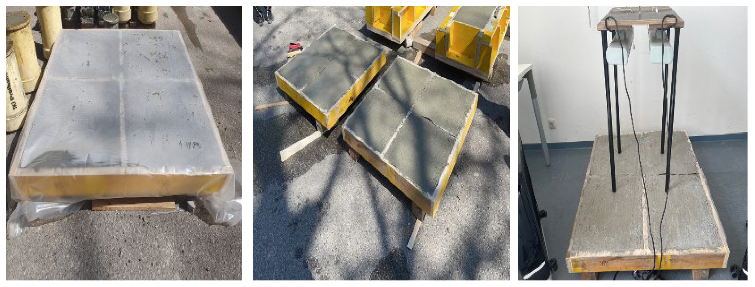
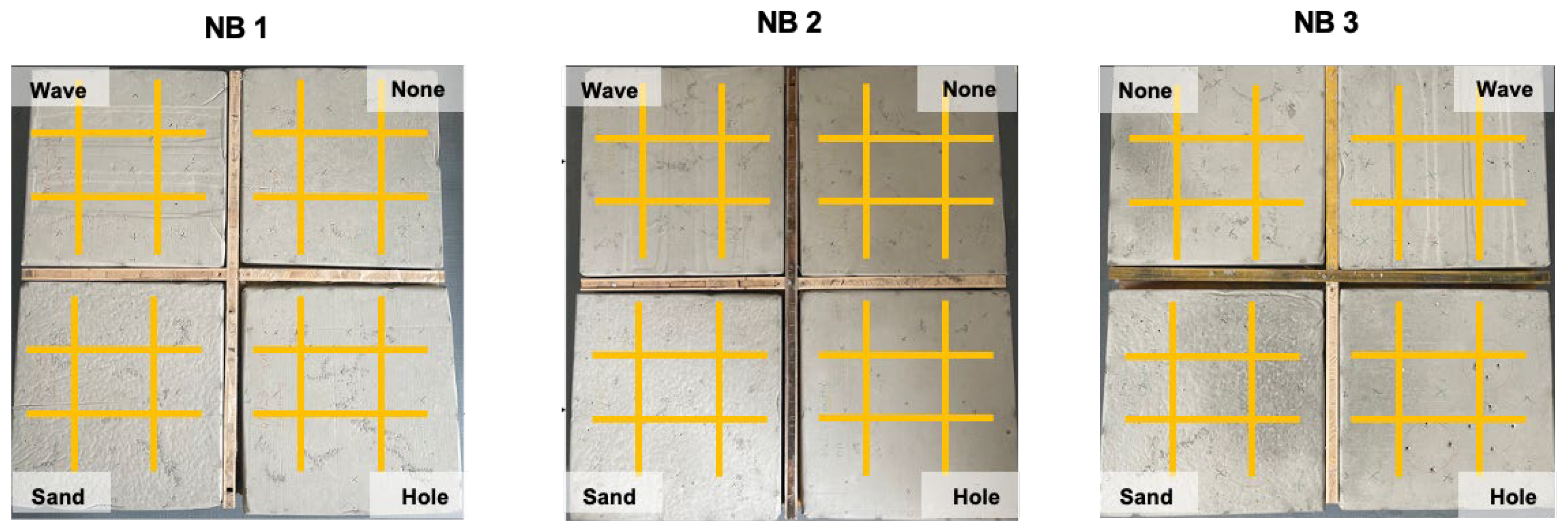
Measurements were taken from the 1st day to the 56th day, every week, after the curing and hardening process, resulting in a total of approximately 1944 HDR images. To focus on the change in spectral signatures over time, samples from four different surfaces, including none, wave, sand, and hole, with three curing treatments (NB1, NB2, and NB3), were recorded using a hyperspectral camera. A total of twelve samples were used, with the spectral mean signatures indicated separately for each day of measurement and observed reflectance development at wavelengths of 600 nm, 650 nm, 700 nm, 750 nm, 800 nm, 850 nm, 900 nm, 950 nm, and 1003 nm, as shown in the bar graph.

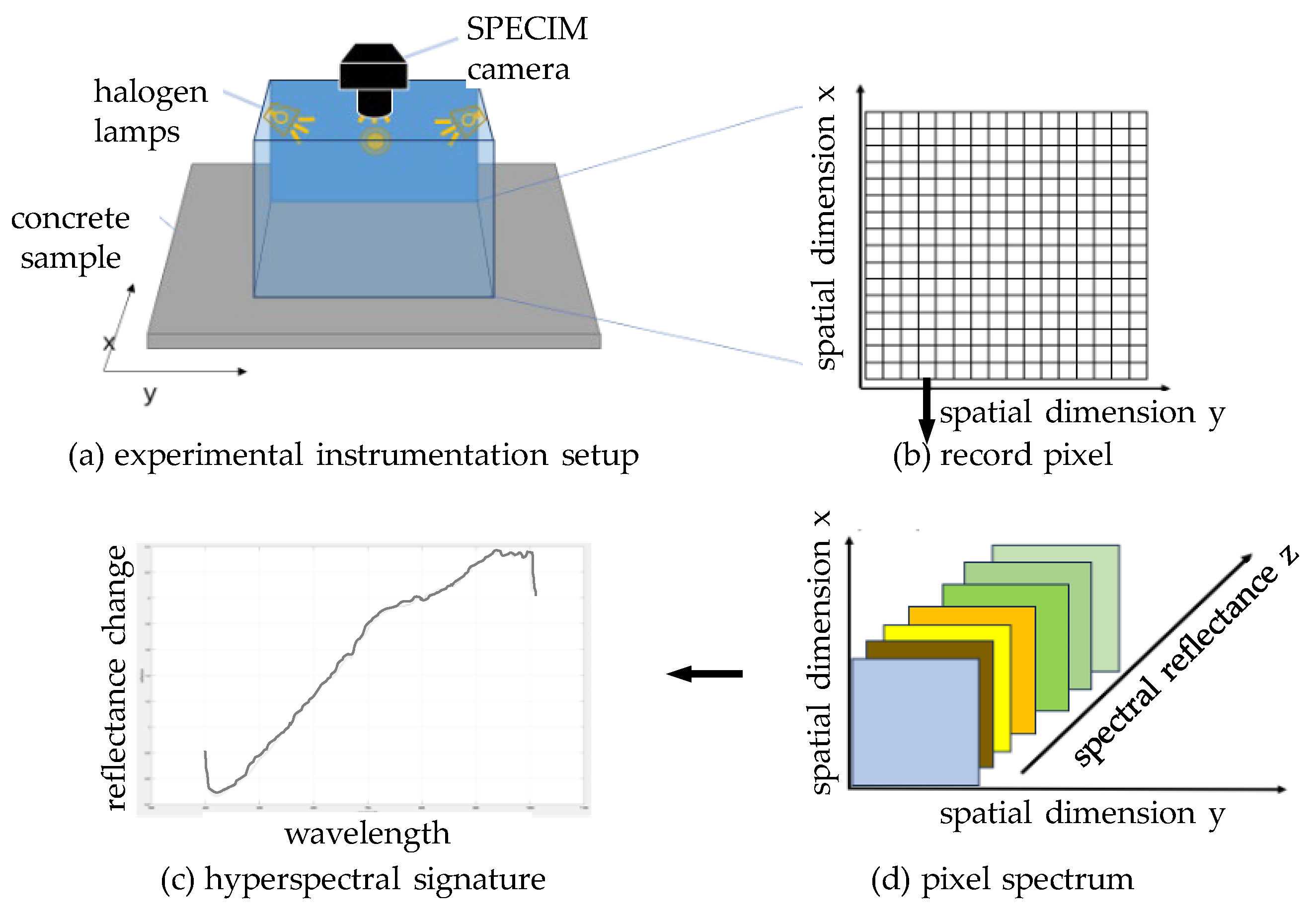
Overall, all hyperspectral signatures in the detected wavelength range (from 392.32 nm to 1003.58 nm) demonstrated a continuous increase in the refraction curve. It was evident that there was a continuous increase in the wavelength range from 392.32 nm to 940 nm, except for a slight decrease around 680 nm and 800 nm (water band), where the reflectance value was clearly visible and fluctuated. Afterward, the reflectance started to decrease sharply from 990 nm to 1003.58 nm.

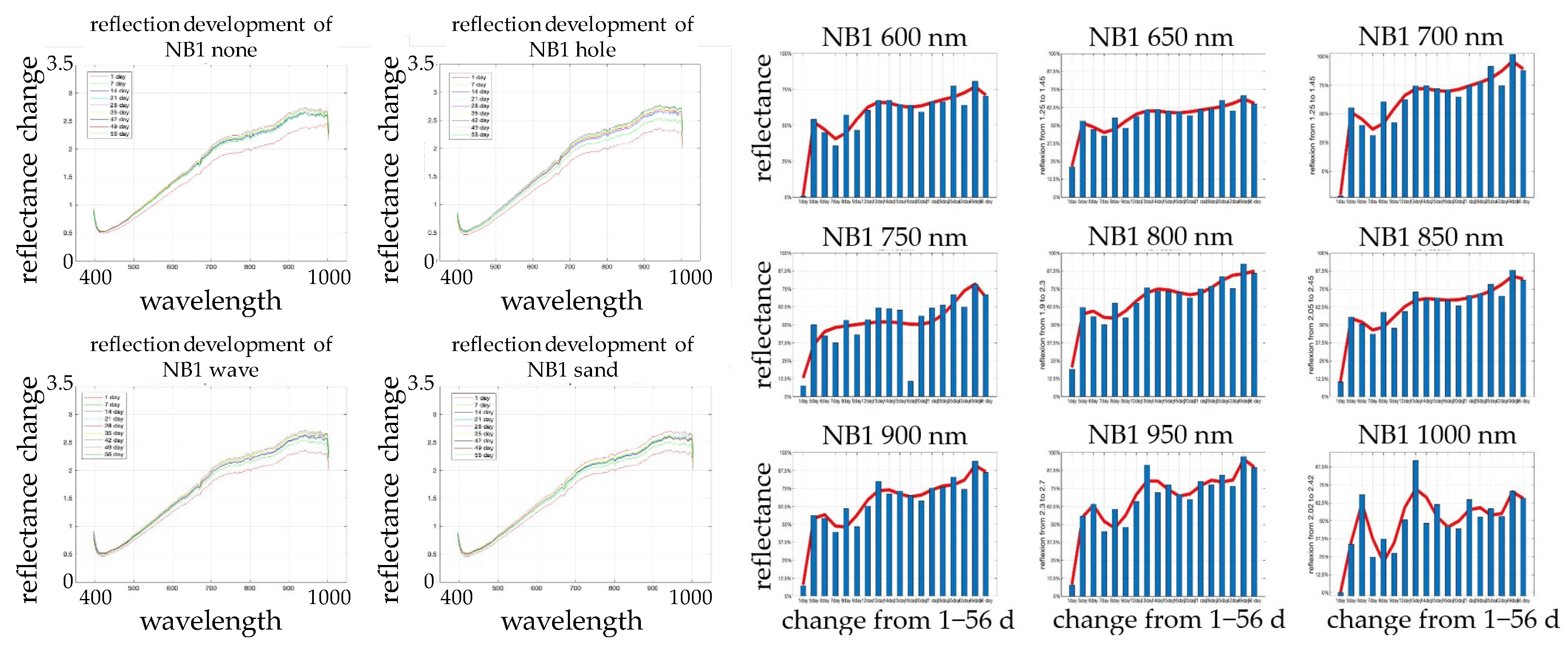
For the concrete sample after the NB1 treatment, as shown in Figure 11(left), the reflectance generally increased significantly with the hydration process, especially on the NB1 hole surface. Meanwhile, the spectral signature on the 35th day was slightly higher than the reflectance on the 42nd day, reaching a peak on the 49th day, rather than the 56th day. Furthermore, Figure 11(right) shows the development in NB1 reflectance over the hydration days. The blue bar represents the true average reflectance value after measurement, while the red curve represents the fitted curve from the 1st day to the 56th hydration day. Due to environmental temperature and water evaporation, the reflectance was lowest on the first day, then reached a small peak on the fifth day before beginning to decrease until the seventh day. Afterward, it started to increase continuously, reaching a second peak on the 13th day, then decreasing from the 13th to the 19th day, and continuing to increase from the 20th day, reaching a maximum value on the 49th day.

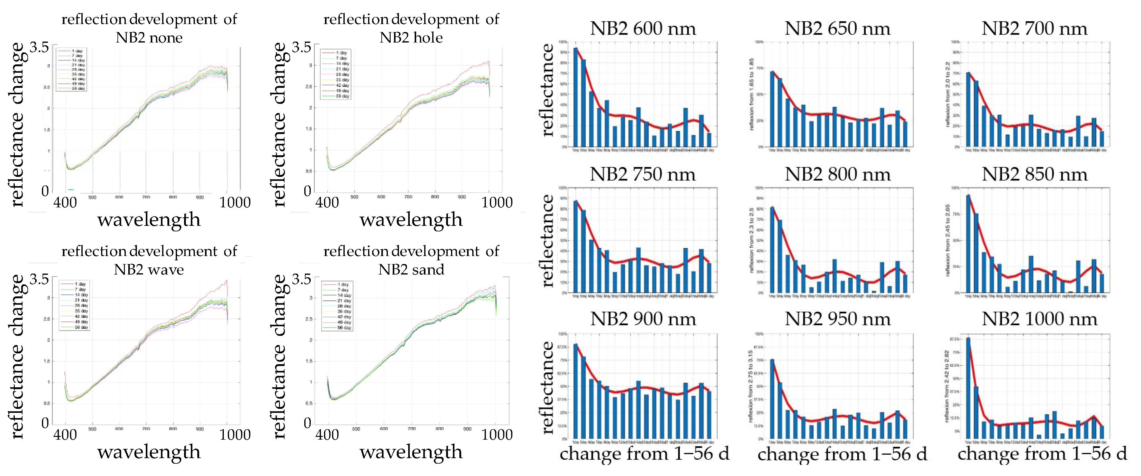
The treated NB2 concrete samples show a significant decrease in the reflectance curve from the 1st day to the 56th day, as shown in Figure 12. There was a slight increase during the second and third weeks. The reflectance of concrete samples with none, wave, and hole surfaces showed very little change over the hydration process, especially in the spectral signature change with the sand surface. The sand surface had a lower reflectance signature compared with other surfaces, while the spectral signature with the hole surface had a higher average reflectance signature. The rate of decline slowed on the 9th day, with a tendency to rebound, showing a slight increase until the 14th day, when it peaked and then fluctuated continuously downward. A trough occurred on the 28th day, followed by a small peak on the 49th day, with a significant reduction in fluctuation. On the other hand, the NB2 samples had consistently lower water content. Therefore, since the NB2 samples were exposed to a higher temperature during the seventh-day preservation, hydration loss was relatively higher, and the lower water content led to the cessation of hydration.

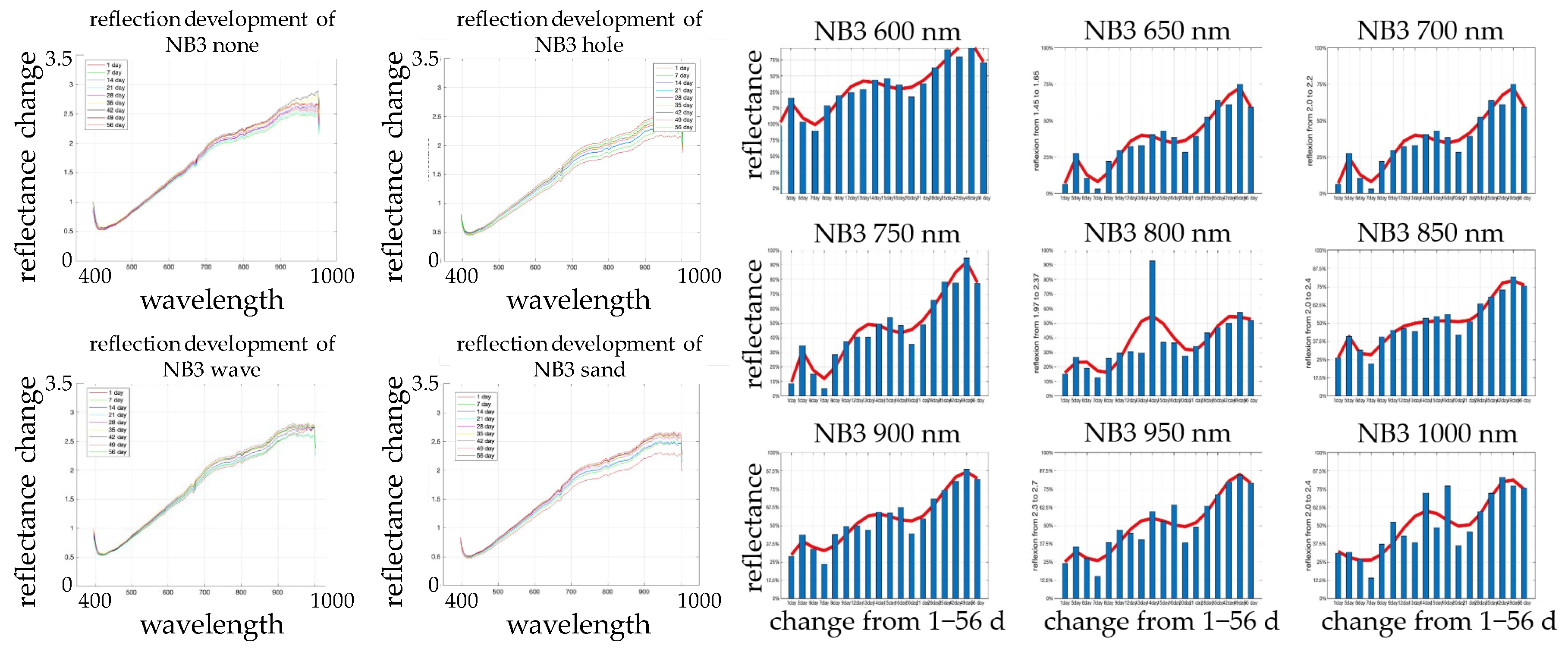
Furthermore, as seen from the NB3 concrete sample in Figure 13, the reflectance increased significantly over the hydration days, while other spectral features remained relatively consistent. In contrast, there was a significant decrease between the 14th and 21st days. However, the spectral characteristics of the NB3 sand surface had a lower reflectance wavelength, while the spectral signature with the hole and wave surfaces had similar reflectance variations. Meanwhile, the overall reflectance of NB3 followed the same trend as NB1, showing a fluctuating increase in reflectance development over the hydration process until reaching the highest emissivity on the 49th day, which was lower than that of NB1. This indicates that cured samples under the NB1 condition had higher water content than those cured under NB3, which suggests better protection for concrete curing under NB1.

3.2. Result Based on Hydration Signatures Classification with Neural Networks

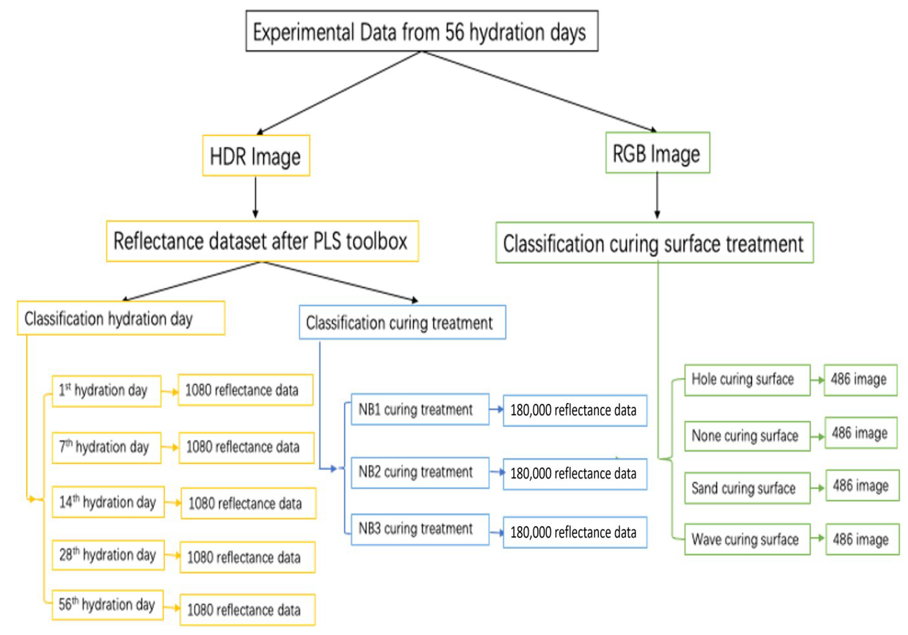
Based on the above contents of hyperspectral analysis, we can better observe the trend in the spectral images and the large database through the HDR image denoising process over the hydration process under three different NB conditions and four different curing surfaces. This also provides a solid foundation for predicting the development of the hydration process with the help of artificial and convolutional neural networks. Therefore, to better predict the concrete hydration process under different treatments, we will utilize the mentioned neural networks to model several networks for a large amount of hyperspectral reflectance data and surface images. This includes classifying the experimental dataset to predict hydration at five different days, three types of NBs, and four types of cured surfaces, as shown in Figure 14.

Table 4 summarizes the performance of the classification models using accuracy, precision, recall, and F1-score. The hydration time prediction task yielded the lowest metrics, whereas the surface classification task demonstrated the highest consistency and robustness across all evaluation indicators.

3.2.1. Hydration Time Classification of Concrete Reflectance Based on CNN Model

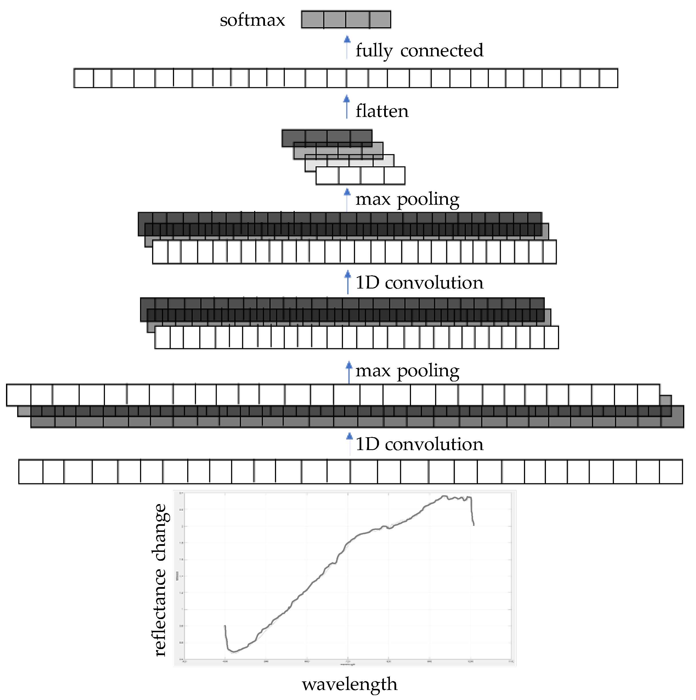
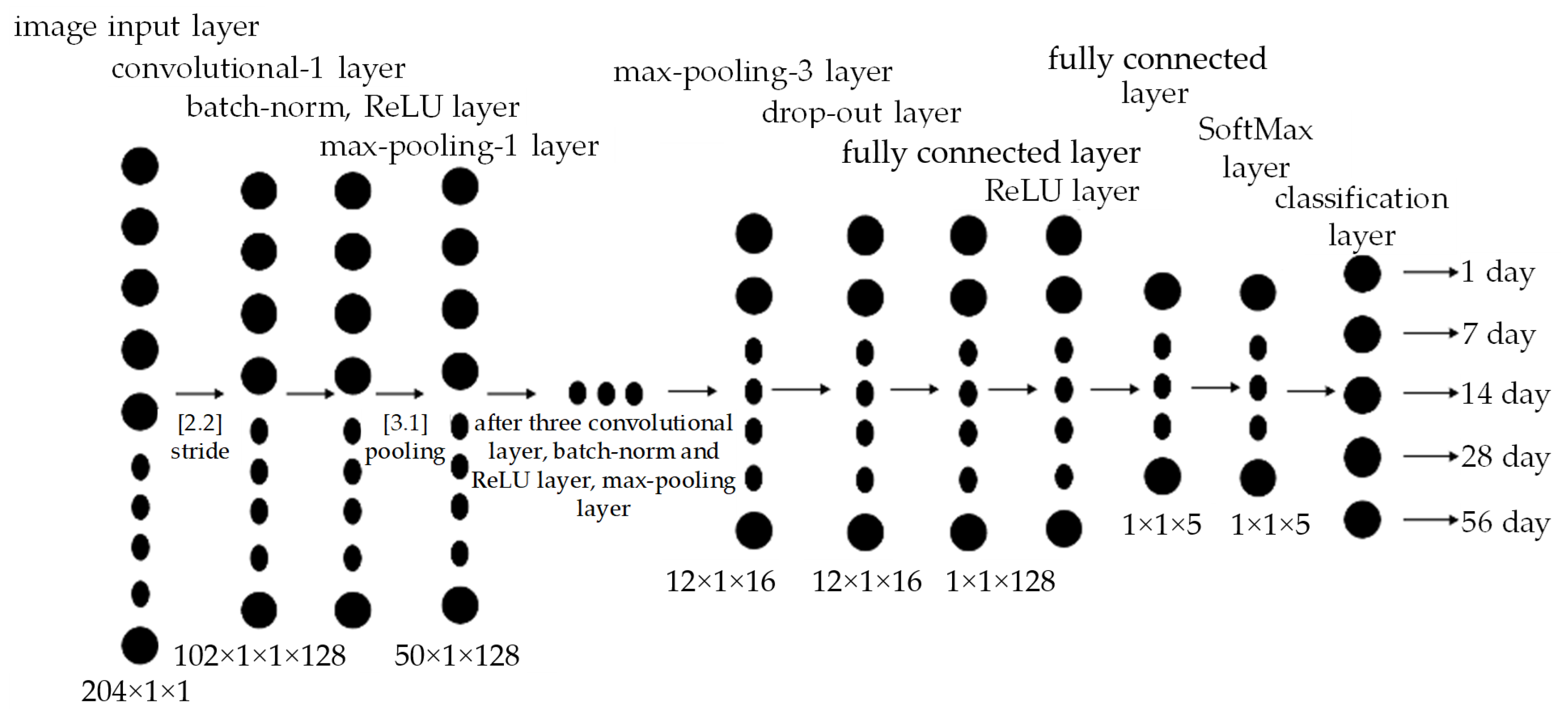
Based on the theoretical neural network method for classification prediction, we aim to process the hyperspectral reflectance dataset of concrete samples for several hydration phases, such as on the 1st, 7th, 14th, 28th, and 56th hydration days, resulting in a total of 540,000 reflectance values. The 540,000 reflectance curves mentioned refer to 12 specimens × 9 sections × 5 hydration ages × 1000 pixels = 540,000 spectral signatures. In addition, the input and output matrices are divided into an 80% training dataset and a test dataset for predicting hydration time, with data randomly selected. Based on the initial values related to certain empirical selections of appropriate hyperparameters, the approximate convergence of the loss function was carefully monitored. The shorter the training time, the better the loss function convergence. After long periods of continuous debugging, the number of iterations was set to 1000, while the training curve oscillated strongly. Meanwhile, when increasing the batch size to 256 and gradually reducing the learning rate, there was a significant improvement in the accuracy. Furthermore, the CNN model structure consists of an input layer, four convolutional layers (each with a batch normalization layer and a ReLU layer), two fully connected layers, and a SoftMax layer and classification layer to achieve hydration time classification and prediction, as shown in Figure 15.

The labelled concrete samples were randomly divided into training and test sets, with 30% of the labelled reflectance datasets used as a validation set to test the model performance of the network for hydration time classification (i.e., accuracy for each category and loss of the neural network). To predict the validation set for the 1st, 7th, 14th, 28th, and 56th hydration days, as shown in Figure 16, it is clear that the prediction of the validation dataset for each period was achieved with an accuracy of 67.8% for hydration time classification.

The relatively modest classification accuracy (67.8%) for hydration time may be attributed to overlapping spectral characteristics in early hydration stages and data imbalance across the five hydration periods. Additionally, the limited use of selected bands may have constrained the model’s feature extraction capacity. Future enhancements could include using more spectral bands, data augmentation, and advanced architectures like residual CNNs or attention-based networks to boost sensitivity and performance.

3.2.2. Curing Treatment Classification of Concrete Reflectance Based on ANN Model

The hyperspectral reflectance data from the concrete samples above were processed for different curing treatments based on ANN classification prediction. A total of 36 HDR images were acquired per curing regime (3 regimes × 12 specimens), and each HDR image contributed 1000 reflectance spectra, resulting in 36,000 values per regime and 108,000 reflectance vectors overall. This means that each NB category would include a total of 204 wavelengths × 108,000 reflectance values, with the output matrix labelling each category as 0, 1, or 2 to represent NB1, NB2, and NB3, respectively.

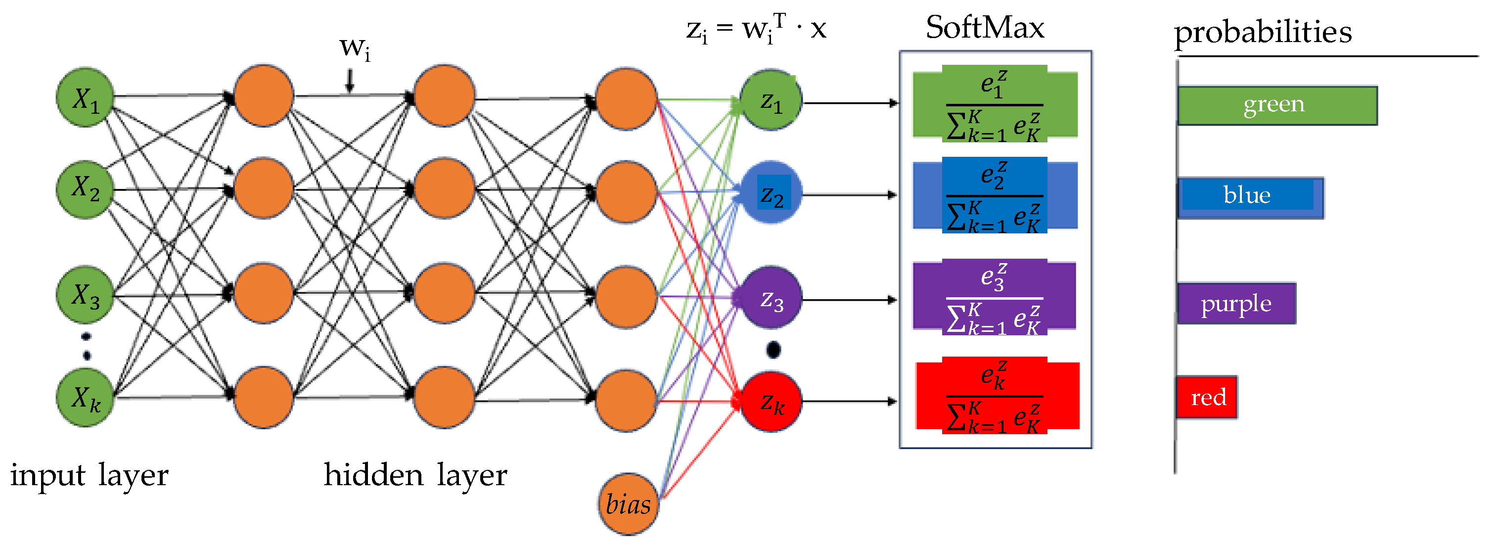
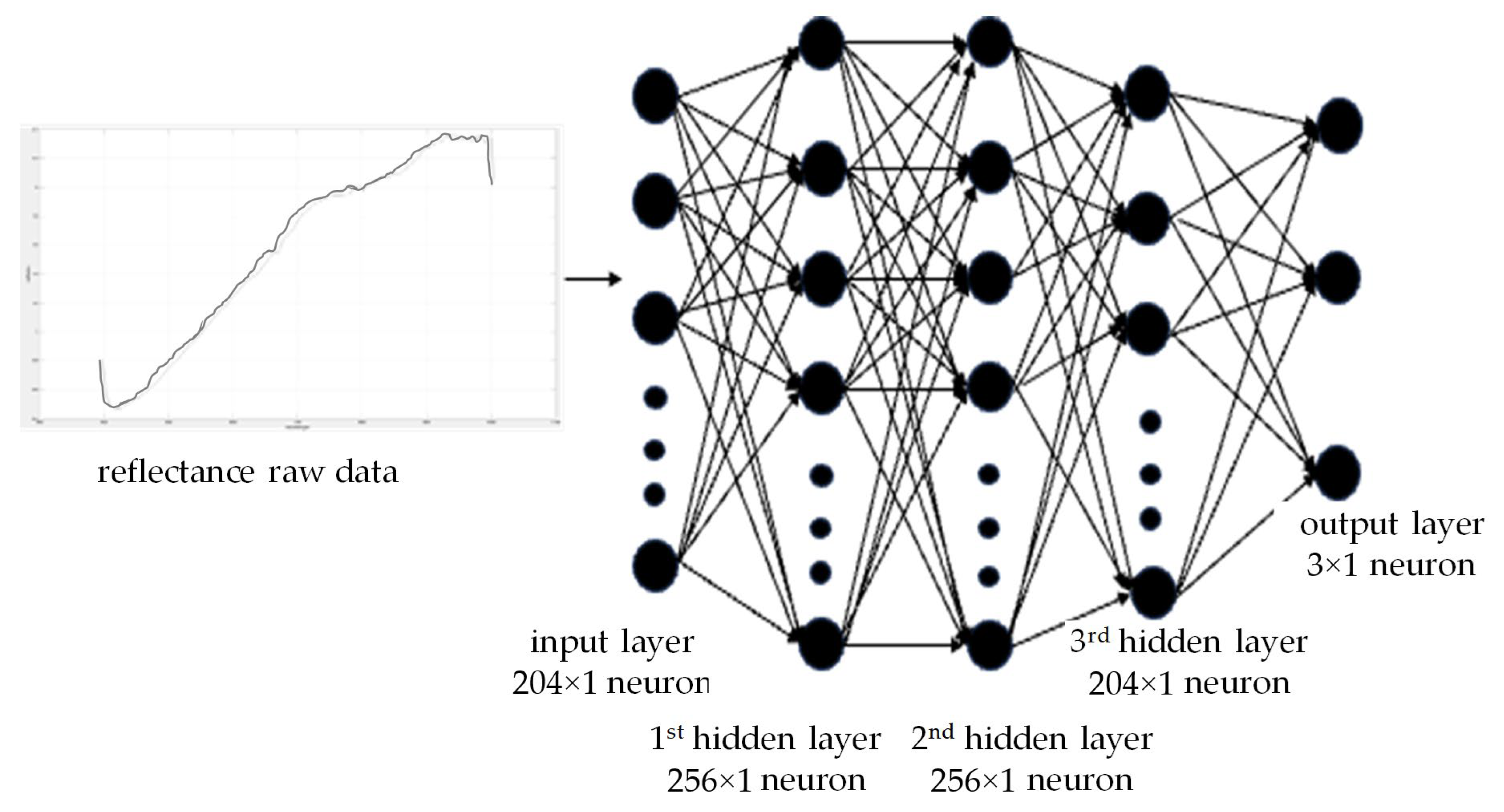
Furthermore, we randomly selected 70% of the total data as the training set to build the ANN prediction model, and the remaining 30% as the validation set to test the accuracy of the model’s classification. For this one-dimensional data, we designed an input layer to accept 204 reflectance values, with four hidden layers for calculations, each including a ReLU activation function, as shown in Figure 17. After a long period of parameter debugging, the appropriate parameters for the ANN model classification were finally adjusted to achieve better prediction performance. The model was iterated 150 times, and the total training time was 26 min and 46 s, using PyCharm CE and the SK-learn toolbox for the ANN model in hydration treatment.

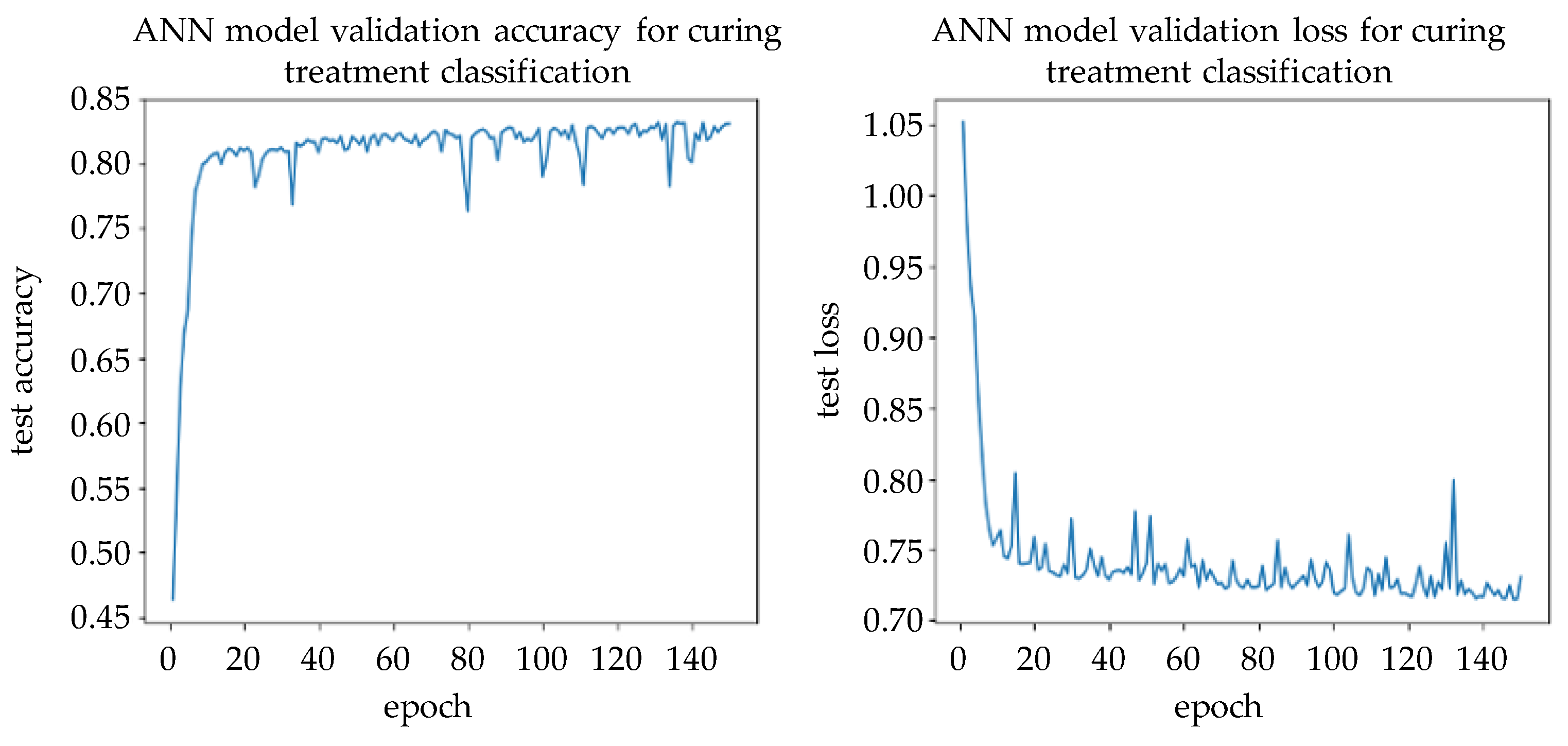
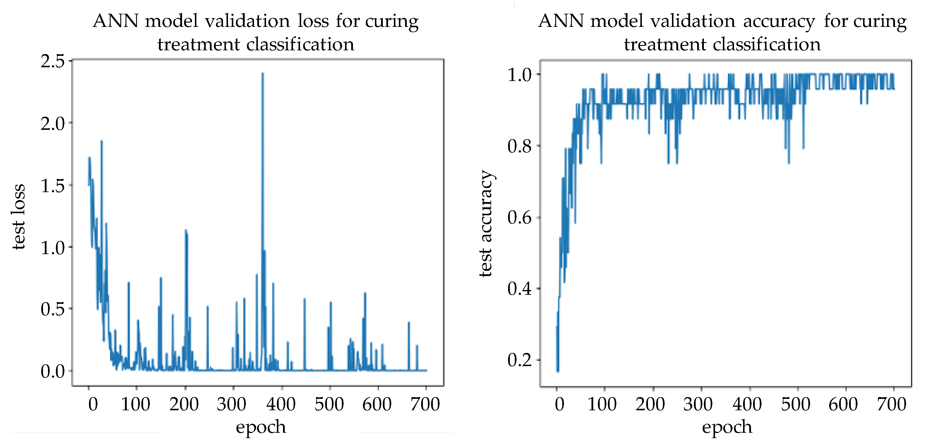
When compared side by side, the figure clearly shows the ANN training process in the left figure and accuracy of around 83.3% on the validation dataset in the right figure for curing NB1, NB2, and NB3 treatment classification and prediction, as shown in Figure 18. It is also clear that the three different NB curing treatments exhibit significant differences in the spectral characteristics of the concrete samples, which provides a solid foundation for determining the concrete quality and differentiating between the three curing treatments.

3.2.3. Curing Surface Classification of Concrete Reflectance Based on CNN Model

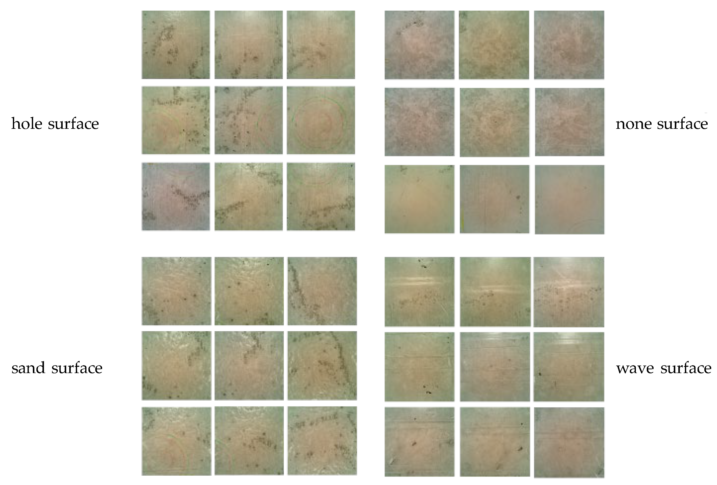
Research on the categorization of different surfaces of concrete samples during the hydration process was carried out, in which nine HDR images and their corresponding RGB images were obtained from experimental data acquisition, as shown in Figure 19. After the entire 56-day hydration observation, a total of 1944 images were captured for four different curing surfaces: hole, none, sand, and wave. These images were labelled into four categories with the help of the CNN model algorithm.

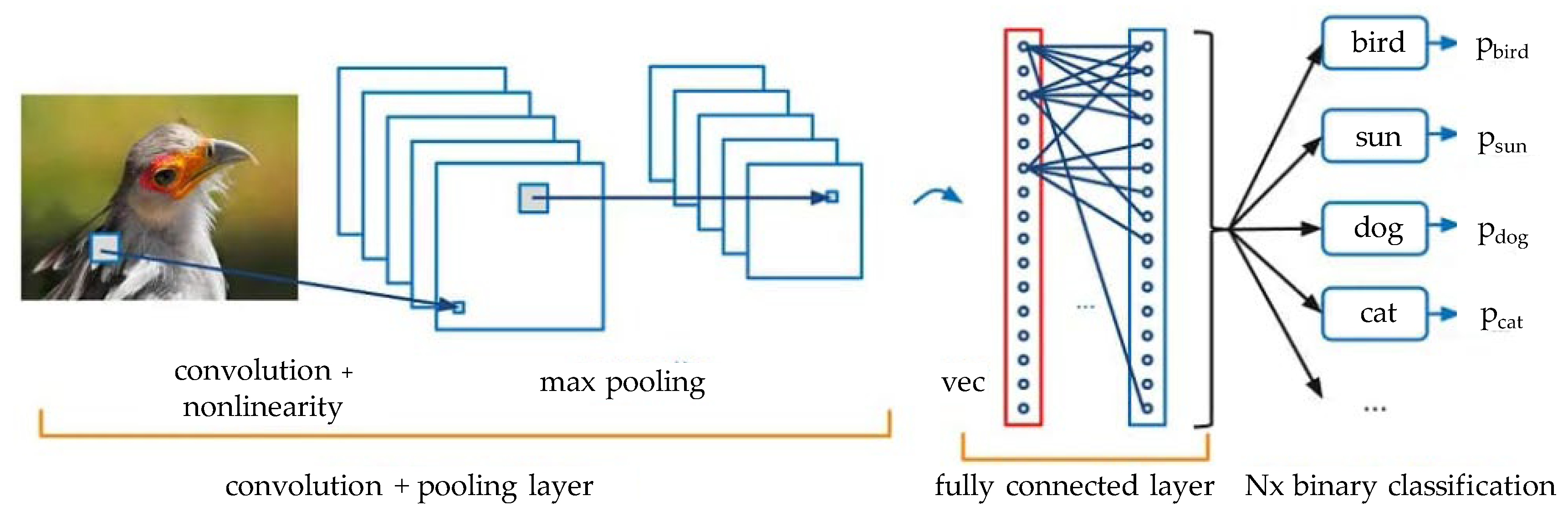
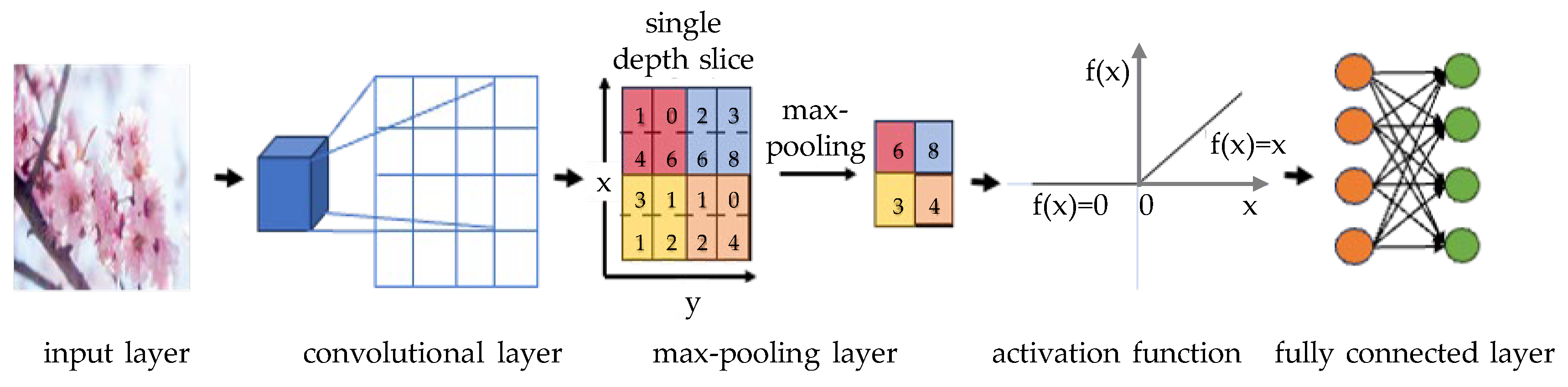
Meanwhile, a CNN model was designed with an input layer, four convolutional layers, pooling layers, a fully connected layer, and a Softmax function. The convolutional layers continuously extracted features from the images, and the pooling layers effectively reduced the size of the feature matrix, decreasing the number of parameters in the final connection layers. As a result, the fewer weight parameters helped speed up the computation and prevented overfitting, as shown in Figure 20.

After training the CNN model with 100 epochs, the total time for training was approximately 1 h, 10 min, and 42 s. Figure 21 shows the results of the validation set for curing surface classification through the CNN model. Furthermore, the loss error of the CNN model was reduced to 0.0001, and the accuracy reached 87.6%. This indicates that the CNN model has strong processing ability for concrete image data and can clearly distinguish between hole, none, sand, and wave concrete curing surfaces.

The model process for the life cycles of curing concrete objects, or even entire infrastructure networks, includes not only inspection (i.e., the survey of the condition) and assessment of structural performance, but also the prediction of hydration maintenance strategies.

These management systems are usually based on deterministic performance prediction models to describe the degradation processes of curing concrete. The increasing use of advanced measurement methods, monitoring technologies, and rapid developments in computer processing have led to a trend towards data-based approaches for curing condition monitoring.

4. Conclusions

It can be demonstrated that the quality of concrete can be classified by comparing hyperspectral data from samples with different curing treatments and hydration periods. It is also possible to classify concrete surfaces by comparing image data of four different concrete surfaces using non-destructive hyperspectral imaging technology. Classification methods using neural networks can more effectively distinguish between concrete samples under three curing treatments, five hydration times, and four surface treatments. Better prediction of concrete quality can be made by analyzing the pattern of hydration reflectance development and surface image data.

Detailed interpretation of the spectral signature statistics for the generated categories and the classification of the hydrated surface image data enabled analysis of the samples from the perspective of the hydration process. Significant changes in hydration time were observed in the hyperspectral data of the analyzed HDR images. Reflectance spectroscopy has developed significantly across the 600–1003.58 nm absorption band. The reflectance values of the water band segment, from 900 nm to 1003.58 nm, show that the NB2 treatment samples have the highest values and, therefore, the highest water content compared to the NB3 treatment samples. This suggests that non-optimally cured samples dry out prematurely, which negatively impacts the developing strength and quality of the concrete. The NB2 curing treatment concrete sample, particularly with the hole surface, has the highest mean reflectance values compared to other surfaces, indicating that the hole surface has a better hydration process, which positively supports the quality of concrete development.

To fit the results of reflectance values in the development over 56 hydration days, it is significant to note that the values of the NB1 treatment samples fluctuate upwards, while those of the NB2 treatment samples fluctuate downwards with the increase in hydration time. This fluctuation likely occurs near the point where water loss becomes more severe. Compared to the NB3 treatment samples, NB1 treatment samples have extreme values at 940 nm, indicating higher water content. Particularly on the 49th day, the highest values were generally reached. Therefore, the best hydration performance is achieved on the 49th day for NB1 curing treatment. In comparison, NB1 provides better curing treatment for protecting the quality of concrete development over a long hydration process.

In the results of CNN classification of hydration times, the distribution of reflectance values clearly distinguishes concrete samples on the 1st, 7th, 14th, 28th, and 56th hydration days. The class distribution of reflectance data can also distinguish NB1 treatment, NB2 treatment, and NB3 treatment with the help of ANN classification. Meanwhile, in the CNN image classification process, the curing surface class distribution of image pixels can significantly differ between concrete samples with none, wave, sand, and hole surface treatments. Classification tests of young concrete on the 1st, 7th, and 14th days gave the clearest results. However, after the 28th day, the hydration changes become less pronounced.

Valuable information on hydration processes, premature drying, and final quality can be obtained from hyperspectral analysis of fresh concrete. From the above experimental analyses, it can be concluded that this method is reliable and promising for assessing the curing quality of concrete specimens.

We hope to further investigate the direct application of this method to structures. A reliable assessment can be achieved by using a reference sample, where the characteristic absorption bands can be used as limits for evaluating curing quality. Measurements are highly dependent on the composition of the concrete and environmental influences such as temperature and humidity. Standardized field tests are, therefore, necessary for reliable assessments using this method. Further investigation of a broader wavelength range is also worthwhile, as it would provide additional information and clearer results.

In this regard, it is hoped that further research in this area will lead to a better understanding of the changing patterns in hydration processes. This understanding could enable the continued assessment of concrete curing and the widespread application of hyperspectral methods in construction practice.

This study is limited by its relatively small sample size (12 specimens) and controlled laboratory conditions. Real-world application of hyperspectral imaging will require calibration under variable lighting, dust, and surface contamination. Additionally, sample diversity (e.g., admixtures, aggregates, formwork effects) was not explored. Future work should focus on in situ testing, expanded datasets, and broader spectral coverage beyond 1000 nm to detect deeper hydration processes. The integration of portable imaging devices with real-time processing could enhance on-site applicability for infrastructure monitoring.

References

1. Rodrıguez-Camacho, R.E.; Uribe-Afif, R. Importance of using the natural pozzolans on concrete durability. Cem. Concr. Res. 2002, 32, 1851–1858. [Google Scholar] [CrossRef]
2. Taylor, H.F.W. Cement-Chemistry, 2nd ed.; Thomas Telford Ltd.: London, UK, 2015. [Google Scholar]
3. Arslan, M.H.; Korkmaz, H.H.; Gulay, F.G. Damage and failure pattern of prefabricated structures after major earthquakes in Turkey and shortfalls of the Turkish Earthquake code. Eng. Fail. Anal. 2006, 13, 537–557. [Google Scholar] [CrossRef]
4. Ptacek, L.; Strauss, A.; Hinterstoisser, B.; Zitek, A. Curing Assessment of Concrete with Hyperspectral Imaging. Materials 2021, 14, 3848. [Google Scholar] [CrossRef]
5. Kim, B.; Cho, S. Automated vision-based detection of cracks on concrete surfaces using a deep learning tech-nique. Sensors 2018, 18, 3452. [Google Scholar] [CrossRef]
6. Manolakis, D.G. Hyperspectral Imaging Remote Sensing: Physics, Sensors, and Algorithms; Cambridge University Press: Cambridge, UK, 2016. [Google Scholar]
7. Pimenidis, E.; Angelov, P.; Jayne, C.; Papaleonidas, A.; Aydin, M. Artificial Neural Networks and Machine Learning—ICANN 2022; Springer Nature Switzerland: Cham, Switzerland, 2022. [Google Scholar]
8. Janiesch, C.; Zschech, P.; Heinrich, K. Machine learning and deep learning. Electron. Mark. 2021, 31, 685–695. [Google Scholar] [CrossRef]
9. Bhatt, D.; Patel, C.; Talsania, H.; Patel, J.; Vaghela, R.; Pandya, S.; Modi, K.; Ghayvat, H. CNN Variants for Computer Vision: History, Architecture, Application, Challenges and Future Scope. Electronics 2021, 10, 2470. [Google Scholar] [CrossRef]
10. Wu, H.; Prasad, S. Convolutional Recurrent Neural Networks forHyperspectral Data Classification. Remote Sens. 2017, 9, 298. [Google Scholar] [CrossRef]
11. Zhang, X.; Li, D.; Zhou, M. Deep learning-based detection of asphalt pavement defects using hyperspectral images. Sensors 2022, 22, 2351. [Google Scholar]
12. Brook, A.; Ben-Dor, E. Reflectance spectroscopy as a tool to assess the quality of concrete in situ. Constr. Technol. 2011, 2, 169–188. [Google Scholar]
13. A Research Guide to Convolutional Neural Networks. Available online: https://fritz.ai/convolution-neural-networks/ (accessed on 3 May 2025).
14. Vagni, F. Survey of Hyperspectral and Multispectral Imaging Technologies (Etude Sur Les Technologies D’imagerie Hyperspectrale Et Multispectrale); Nato Research And Technology Organization Neuilly-Sur-Seine: Neuilly-sur-Seine, France, 2007. [Google Scholar]
15. Mozgeris, G.; Juodkienė, V.; Jonikavičius, D.; Straigytė, L.; Gadal, S.; Ouerghemmi, W. Ultra-Light Aircraft-Based Hyperspectral and Colour-Infrared Imaging to Identify Deciduous Tree Species in an Urban Environment. Remote Sens. 2018, 10, 1668. [Google Scholar] [CrossRef]
16. Eigenvector, Chemometrics—Data Analysis Software—PLS_Toolbox—Eigenvector. Available online: https://eigenvector.com/software/pls-toolbox/ (accessed on 15 August 2023).
17. Fan, L.; Fan, M.; Alhaj, A.; Chen, G.; Ma, H. Hyperspectral imaging features for mortar classification and compressive strength assessment. Constr. Build. Mater. 2020, 251, 118935. [Google Scholar] [CrossRef]
18. Ma, P.; Fan, L.; Chen, G. Hyperspectral reflectance for determination of steel rebar corrosion and Cl− concentration. Constr. Build. Mater. 2023, 368, 130506. [Google Scholar] [CrossRef]
Figure 1. Architecture of neural network.
Infrastructures 10 00172 g001
Figure 2. Imaging data analysis in convolutional neural networks [9].
Infrastructures 10 00172 g002
Figure 3. Feature computation for RGB image in convolutional layer.
Infrastructures 10 00172 g003
Figure 6. (left) NB1 treatment under 20 °C with foil; (middle) NB2 treatment under 20 °C without foil; (right) NB3 treatment under 40 °C without foil.
Infrastructures 10 00172 g006
Figure 7. (left) Concrete samples after NB1 with none, wave, sand, and hole surface; (middle) concrete samples after NB2 with none, wave, sand, and hole surface; (right) concrete samples after NB3 with none, wave, sand, and hole surface.
Infrastructures 10 00172 g007
Figure 8. Experimental setup table for the HDR image acquisition.
Infrastructures 10 00172 g008
Figure 9. HDR imaging recording process and data extraction.
Infrastructures 10 00172 g009
Figure 10. Experimental dataset in 56 hydration days of concrete sample.
Infrastructures 10 00172 g010
Figure 11. (Left) Mean spectral reflectance for NB1 samples with four surface treatments from day 1 to day 56. (Right) Temporal evolution of reflectance at selected wavelengths (600–1003 nm). Y-axis: reflectance (%); X-axis: hydration days.
Infrastructures 10 00172 g011
Figure 12. (Left) Mean spectral reflectance for NB2 samples with four surface treatments from day 1 to day 56. (Right) Temporal evolution of reflectance at selected wavelengths (600–1003 nm). Y-axis: reflectance (%); X-axis: hydration days.
Infrastructures 10 00172 g012
Figure 13. (Left) Mean spectral reflectance for NB3 samples with four surface treatments from day 1 to day 56. (Right) Temporal evolution of reflectance at selected wavelengths (600–1003 nm). Y-axis: reflectance (%); X-axis: hydration days.
Infrastructures 10 00172 g013
Figure 14. Raw data for the three classification models.
Infrastructures 10 00172 g014
Figure 15. CNN layer structure of hydration time prediction.
Infrastructures 10 00172 g015
Figure 16. Accuracy result of validation dataset for hydration time classification.
Infrastructures 10 00172 g016
Figure 17. ANN model for curing treatment classification.
Infrastructures 10 00172 g017
Figure 18. (left) Accuracy result of validation test for curing treatment classification; (right) loss result of validation test for curing treatment classification.
Infrastructures 10 00172 g018
Figure 19. Image dataset example for curing surface treatment classification.
Infrastructures 10 00172 g019
Figure 20. CNN architecture for curing surface classification.
Infrastructures 10 00172 g020
Figure 21. (left) Loss result of validation set for curing surface classification; (right) accuracy result of validation set for curing surface classification.
Infrastructures 10 00172 g021