Experimental and Numerical Model Analysis of Pipe–Soil Interaction Under Typical Geohazard Conditions

Abstract

This paper systematically investigates the interaction between pipes and soil under geo-logical disaster conditions by combining small-scale physical experiments with mul-ti-method numerical simulations. Three analytical models—namely the Smoothed Particle Hydrodynamics-Finite Element Method (SPH-FEM) model, the traditional FEM model, and the soil spring-based Pipe–Soil Interaction (PSI) model—are employed to comparatively analyze their applicability across different geohazard scenarios. The study found that the PSI model overpredicted pipeline strain responses, indicating that traditional soil spring analytical models require modification. The traditional FEM model provided the most accurate predictions under small-displacement conditions, while the SPH-FEM model yielded more reliable results for large-displacement scenarios. The novelty of this study lies in its systematic exploration of the applicability of these three methodologies, providing scientifically grounded simulation tools for numerical modeling in engineering practice.

1. Introduction

Oil and gas pipelines inevitably traverse some areas with high incidence of geological hazards. During the occurrence of geological disasters, the surrounding soil of pipelines will experience large-scale displacement and deformation [1]. The permanent ground deformation causes pipelines to undergo significant deformation and displacement under the action of surrounding soil pressure, affecting pipeline safety [2]. With the development of theoretical research and computer technology, various numerical simulation methods have been widely applied in the analysis of pipe–soil interaction. Compared with theoretical analytical methods, numerical methods can better describe the nonlinearity of pipe–soil interaction and have gradually become the mainstream research method [3]. Currently, the primary finite element numerical models currently include nonlinear soil spring models, traditional FEM (Finite Element Method, FEM) models, and SPH-FEM (Smooth Particle Hydrodynamics-Finite Element Method, SPH-FEM) coupled models.

The finite element numerical simulation model based on soil springs was the earliest approach employed for the numerical modeling of pipe–soil interaction. In 2001, Lim et al. [4] established a numerical model using beam elements to represent pipelines and a series of elastoplastic springs uniformly distributed along the pipe circumference to simulate the surrounding soil. This model analyzed the mechanical response of buried pipelines subjected to lateral spreading displacements induced by soil liquefaction, investigating the influence of parameters such as pipe diameter and wall thickness. Their work proposed critical values for lateral spreading length and peak ground displacement at local buckling failure. In the same year, Takada et al. [5] developed a beam–shell coupling model, where shell elements were used for pipe segments within a limited range on both sides of the fault zone while beam elements represented other sections. This approach maintained computational accuracy while improving efficiency. Through this model, they analyzed the relationship between maximum pipe strain and crossing angle. In 2011, Xie et al. [6] conducted a comparative analysis of three modeling approaches: pipe–soil spring, shell-soil spring element, and continuum soil–shell element models. Their results demonstrated minor differences in local pipe deformation predictions among these methods. In 2012, Zhang et al. [7] established a soil-spring-based pipe–soil model to simulate and analyze the mechanical response of pipelines under two types of mining-induced subsidence: trough settlement and foundation pit settlement. In 2022, Ji [8] created a numerical model of pipe–soil interaction using the nonlinear soil spring method, examining the displacement and axial stress distribution of X80 pipelines under various forms of collapse and subsidence-induced ground movements. To date, soil-spring-based numerical simulation methods remain widely used in pipeline engineering practice.

The soil spring model demonstrates significant advantages in simulating large-scale pipe–soil interaction, yet exhibits notable limitations in characterizing localized contact behavior. In contrast, continuum FEM models have proven more effective for simulating pipe–soil contact behavior and have been successfully applied to analyze pipeline responses under typical geohazards including subsidence, landslides, and fault movements. Early scholars employed traditional FEM models for such analyses, which were based on solid elements. Zhao et al. [9] investigated the effects of varying settlement magnitudes and ranges on pipeline bending stress, identifying stress concentration primarily at inflection points of the settlement profile. Tang et al. [10] studied buckling and failure mechanisms during landslide progression, confirming localized buckling as a primary failure mode in early-stage pipeline damage. Karamitros [11] utilized 3D FEM to examine pipe–soil interaction at normal faults, revealing that traditional models struggled to accurately simulate complex soil-pipe contact behavior, thereby compromising mechanical response predictions. These models have also been extended to other geohazard scenarios. However, constrained by the deformation capacity of traditional FEM meshes, the SPH-FEM coupling model has recently gained attention for its superior capability in modeling large soil deformations. Zhang et al. [12] applied SPH-FEM model to simulate pipe–soil interaction during landslides and collapses, with results demonstrating the model’s accuracy in capturing large-deformation soil characteristics.

While researchers have employed various finite element models to investigate pipe–soil interaction under different geohazard scenarios, existing studies remain limited to applying single modeling approaches to individual hazard types. Notably, no systematic comparative analysis has been conducted across multiple geohazards using the aforementioned FEM methodologies, nor have the discrepancies and accuracy of different finite element models in predicting pipeline mechanical responses been quantitatively evaluated. This study establishes a horizontal comparison framework for soil spring models, traditional FEM, and SPH-FEM coupled models to evaluate the applicability of nonlinear soil spring models and continuum solid models in analyzing pipe–soil interactions under three typical geohazard scenarios (collapse, landslide, and fault displacement), aiming to address existing research gaps. The findings provide empirical evidence for researchers to select reliable numerical simulation methods in pipeline integrity assessments.

2. Pipe–Soil Interaction Test Apparatus

2.1. Apparatus Introduction

To investigate the mechanical response characteristics of buried pipelines under fault, settlement, and landslide conditions, and to provide calibration and verification data for numerical models, a pipe–soil interaction test apparatus capable of simulating these three types of geological hazard scenarios was designed and constructed. By measuring the displacement response of UPVC pipes under different geological conditions, a comparison benchmark between physical experiments and numerical simulations was established. The test platform consists of a sandbox, steel frame, movable base plate, and hydraulic lifting platform. The sandbox has dimensions of 1500 mm (length) × 500 mm (width) × 515 mm (height), is made of transparent acrylic glass, and has a thickness of 20 mm. The three-segment structural design allows for adjustments to the steel frame and hydraulic platform positions depending on the test scenario. For fault displacement or settlement tests, the sandbox is placed on the hydraulic platform, while for fixed conditions, it is secured to the steel frame. Holes are drilled on both sides of the sandbox at 0.2 m above the base, with flanges installed externally. The test pipeline passes through these flanges and is bolted in place. The maximum designed burial depth of the pipeline is 0.3 m.

Strain gauges were installed along the axial direction at the top of the test pipeline (or on the slope-facing side for landslide conditions). After assembling the test setup, soil was filled into the sandbox in 50 mm layers, with each layer compacted using a tamping plate to ensure soil density. This layer-by-layer filling and compaction process continued until reaching the pipeline installation depth (200 mm soil depth). At this stage, the test pipeline was positioned on the test frame and secured at both ends with bolts to prevent rotation or sliding during subsequent soil filling. After pipeline fixation, the soil adjacent to the pipe was gently compacted, and filling continued using the same method until reaching the target burial depth. Sensor wiring was routed out during filling and connected to the strain data acquisition system. For both fault displacement and soil settlement tests, the pipeline centerline burial depth was maintained at 0.3 m. In the lateral landslide test, an inclined slope was created within the sandbox to simulate natural slope conditions, following the same layered compaction process, with a pipeline burial depth of 70 mm (Figure 1b). Figure 2 illustrates the implementation methods for different soil displacement modes.

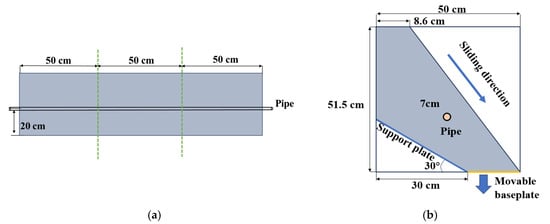
Figure 1. Diagram of pipe–soil interaction test apparatus: (a) Front view; (b) side view.

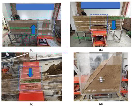
Figure 2. Experimental simulation methods for different geohazard types: (a) Fault; (b) settlement; (c) landslide; (d) fixed-end.

2.2. Test Materials

2.2.1. Test Pipe

Due to the high stiffness of metal pipelines, which results in minimal deformation under small-scale soil interactions, this experiment comprehensively considered factors such as size, operability, and data accessibility, ultimately selecting (Unplasticized Polyvinyl Chloride) UPVC pipes as the test pipelines. The mechanical and dimensional parameters of the chosen UPVC pipes are presented in Table 1. The pipe material parameters were obtained from manufacturer-certified data.

Table 1. Parameters of UPVC pipes for test.

Density	Elasticity Modulus	Poisson’s Ratio	Length	Diameter	Thickness
1400 kg/m3	3500 MPa	0.38	2 m	25 mm	1.5 mm

2.2.2. Test Soil

For this experiment, backfill soil from the pipe trench was selected, classified as silty sand with no gravel or other impurities present. After soil filling, direct shear test specimens were prepared in strict compliance with the Chinese National Standard GB/T 50123-2019 “Standard for Geotechnical Testing Methods” [13]. The direct shear tests yielded a soil internal friction angle of 34.6° and cohesion of 1210 Pa. Soil density was measured using a density ring apparatus, with three replicate tests conducted to determine an average density value of 1631 kg/m³.

2.3. Data Acquisition Device and Monitoring Protocol

2.3.1. Data Acquisition Device

Resistance strain gauges (Model: BE120-3AA-P300) were used to measure the axial strain of the pipeline during the test. The resistance strain gauges had a resistance value of 120.2 ± 0.1 Ω and a maximum range of 20,000 με. The strain gauges were connected to the strain acquisition instrument using a three-wire self-compensation method, suitable for measuring axial strain caused by simple tension, compression, or bending.

The strain data acquisition was performed using the Donghua Test DH3861N Static Stress-Strain Test and Analysis System. This static strain acquisition instrument has a maximum acquisition frequency of 5 Hz and a strain range of ±60,000 με, with a minimum resolution of 0.1 με, making it suitable for indoor quasi-static tests. The acquisition instrument has 72 measurement channels, each of which can be independently connected to different bridge types. During measurement, the system was controlled via computer software to achieve real-time data acquisition. Train gauges and the data acquisition instrument are illustrated in Figure 3.

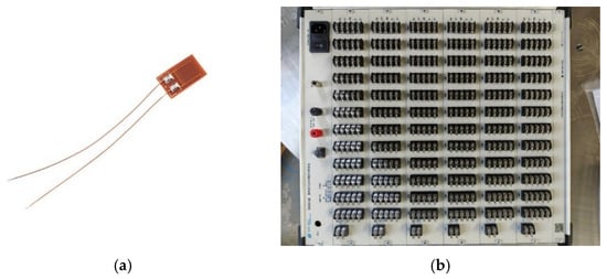
Figure 3. Resistance strain gauge and data acquisition instrument: (a) Resistance strain gauge; (b) data acquisition instrument.

2.3.2. Monitoring Protocol

The strain measurement point arrangements for the settlement test and fault displacement test pipelines are illustrated in Figure 4 and Figure 5. Resistance strain gauges were uniformly spaced at 0.15 m intervals along the pipeline crown (top surface) in the axial direction, with a total of 10 gauges installed. The strain gauge layout for the lateral landslide test pipeline is shown in Figure 4, where gauges were mounted at 0.15 m intervals along both the upslope and downslope surfaces in the axial direction. This configuration enables measurement of axial strain variations under different soil displacement conditions. The strain gauges were bonded to the test pipeline surface using CYANOACRYLATE 502 instant adhesive, ensuring complete surface adhesion. To protect against moisture ingress and mechanical damage from soil movement during testing, each installed gauge was coated with a protective layer of K-704 N silicone sealant for waterproofing and abrasion resistance after achieving proper surface contact.

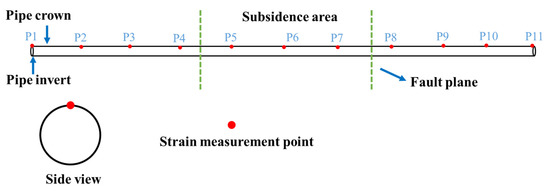
Figure 4. Strain Gauge Layout Plan for Soil Settlement and Reverse Fault Tests.

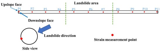
Figure 5. Strain Gauge Layout Plan for Landslide Experiment.

3. Pipe–Soil Interaction Test Results

3.1. Test Results Under Fault Action

The pipe–soil interaction test under reverse fault conditions was conducted by applying a 200 mm vertical upward displacement to the left-side container. Soil deformation patterns at varying fault displacement stages are presented in Figure 6. When the fault displacement reached 20 mm, soil cracks initiated on the fault plane and its left side. A triangular fracture zone developed at the crown of the pipe in the footwall block. With increasing displacement, the cracking intensity progressively intensified, the affected zone expanded, and the fracture zone became more pronounced.

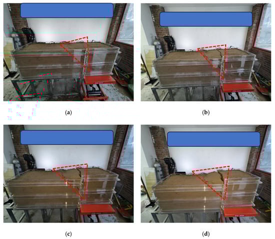
Figure 6. Soil Deformation During Fault Tests: (a) 25 mm displacement; (b) 50 mm displacement; (c) 75 mm displacement; (d) 100 mm displacement.

The measured axial strain at the pipe crown under varying fault displacements is presented in Figure 7. Strain concentrations were confined within ±0.5 m of the fault plane during movement. In the moving block, tensile strain developed at the pipe crown, while the stationary block exhibited compressive strain. As fault displacement increased, tensile strain magnitude progressively exceeded compressive values, with the disparity widening—indicating global pipeline tension. Maximum tensile strain reached 1.12% at monitoring point S8 (0.05 m right of fault plane), whereas peak compressive strain of −0.39% occurred at S6 (0.25 m left). The radial distribution of peak strain expanded with displacement, though strain growth rate diminished beyond 75 mm displacement. Notably, compressive strain at S6 stabilized between 75–100 mm displacements due to coupled bending-stretching deformation mechanisms.

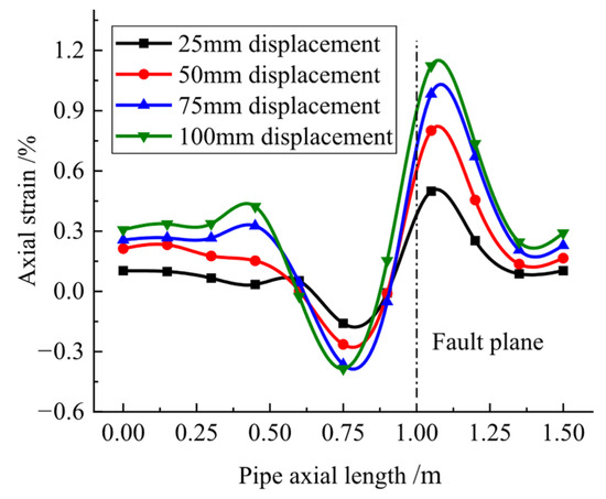
Figure 7. Axial Strain Distribution Curves at Pipeline Crown Under Fault Displacement.

3.2. Test Results Under Settlement Action

The soil settlement simulation test was conducted with a maximum applied displacement of 50 mm. Soil deformation patterns during the test are illustrated in Figure 8 and Figure 9. The settlement zone exhibited continuous downward movement under gravity, with deformation continuity maintained by the constraining effect of rubber bearing pads. At approximately 12 mm maximum settlement, distinct tensile cracks initiated laterally along the settlement boundaries. Internal soil deformation around the pipeline was tracked using a lime powder marker on the sidewalls, revealing progressively increasing settlement magnitudes from upper to lower soil strata. When displacement reached 50 mm, these cracks propagated fully downward, forming through-going fractures to the base layer.

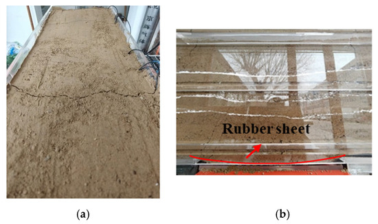
Figure 8. Soil Behavior Under 25 mm Settlement Displacement: (a) Soil surface; (b) settlement area.

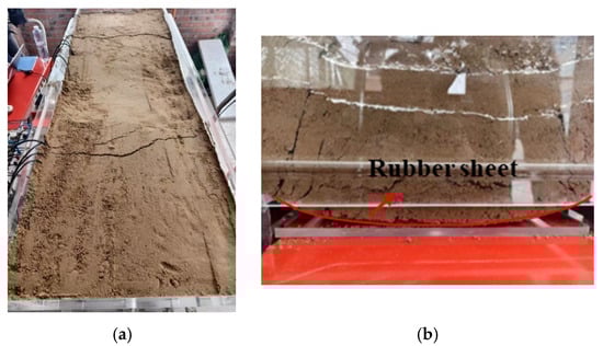
Figure 9. Soil Behavior Under 50 mm Settlement Displacement: (a) Soil surface; (b) settlement area.

The measured axial strain values of the pipeline at different settlement magnitudes are shown in Figure 10. The axial strain distribution along the pipeline was approximately symmetric about the mid-span cross-section. Within the settlement zone, compressive stress acted on the pipe crown, while tensile stress dominated on both sides. The extreme axial strain values were located at monitoring point S6 at the pipeline mid-span and points S4/S8 outside the settlement zone. Both the axial strain values and the range of extreme strain responses gradually increased with greater settlement magnitudes. At 25 mm settlement, the maximum axial tensile strain was 0.2% at monitoring point S8 on the outer edge of the settlement zone, while the maximum axial compressive strain was 0.22% at mid-span point S6. When the settlement reached 50 mm, the maximum axial tensile strain increased to 0.31% and the maximum axial compressive strain reached 0.33%.

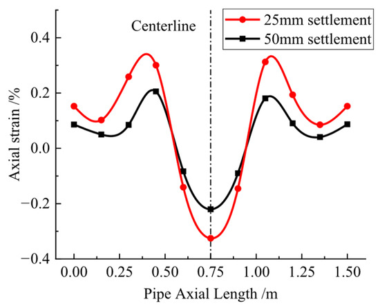
Figure 10. Axial Strain Curves at the Pipe Crown During Different Settlement Stages.

During the tests, vertical displacements at the soil base were measured under 25 mm and 50 mm imposed settlements. Horizontal displacement measurements were recorded at 25 mm intervals across the test section. The measured settlement profiles for both 25 mm and 50 mm cases are tabulated in Table 2, with the pipeline mid-span designated as the coordinate origin (x-axis: horizontal distance; y-axis: settlement magnitude). The experimental data were fitted using Fourier series expansion to derive soil displacement functions for both settlement scenarios. The resulting settlement curves were subsequently implemented as boundary conditions in the finite element model.

Table 2. Measurement Value of Soil Settlement Displacement.

Horizontal Coordinate/mm	Settlement
	25 mm	50 mm
−250	0	0
−200	8.58	17.06
−150	15.67	30.52
−100	21.10	40.69
−50	23.60	46.98
0	25.00	50.00
50	23.58	46.80
100	20.64	40.25
150	15.21	30.12
200	8.47	16.95
250	0	0

The settlement curve functions for the two working conditions are as follows:

$$W(x)=-45.83+95.08\cos 0.0043x-0.14\sin 0.0043x$$

(1)

$$W(x)=-40.78+65.65\cos 0.0036x-0.16\sin 0.0036x$$

(2)

where W(x) is the settlement magnitude (in millimeters) at location x, m.

3.3. Test Results Under Landslide Action

The constructed physical model for the lateral landslide pipe–soil test is shown in Figure 1b. Figure 11 details the deformation and failure states of the landslide mass at different stages. The stability of the soil mass was disrupted by downward movement of the base plate at the landslide toe, inducing soil slippage along the slope surface. Given the pipeline’s substantially higher stiffness compared to the soil, significant deformation incompatibility occurred. The obstructing effect of the pipeline caused markedly greater soil displacement beneath the pipe than above it. As sub-pipe soil displacement increased, tension cracks initiated at the pipe-landslide interface and progressively expanded, disrupting the continuity of landslide movement. The soil beneath the pipeline gradually separated from the pipe surface, resulting in progressive loss of soil support and ultimately creating a suspended pipe segment within the landslide zone.

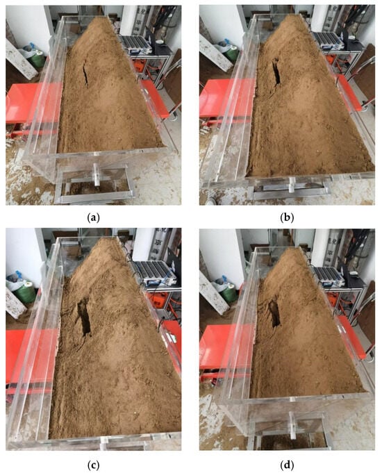
Figure 11. Soil Deformation During Landslide Tests: (a) Baseplate descends by 25 mm; (b) baseplate descends by 50 mm; (c) baseplate descends by 75 mm; (d) baseplate descends by 100 mm.

The axial strain distribution on the landslide-facing pipe surface was measured at different stages of the test, as shown in Figure 12. The strain profile exhibited approximate symmetry about the mid-span plane, though the right-side strain magnitudes were systematically higher than the left-side values due to greater soil deformation on the landslide’s right flank. This observation aligned with the physical test results and was attributed to unavoidable soil heterogeneity in experimental conditions. Under lateral landslide loading, the axial strain distribution pattern resembled that induced by soil settlement. Compressive strain dominated within the landslide-affected zone, while tensile strain developed in the anchored pipe segments outside the slide boundaries. The peak strain values were concentrated in two regions: the central portion of the landslide zone and the transition areas near the landslide boundaries. As landslide displacement increased, the pipe axial strain exhibited progressive growth. However, the strain increment rate decreased significantly after Stage 2. By Stage 4, the three peak strain values showed minimal variation (less than 5%) compared to Stage 3, indicating strain stabilization. This behavioral transition coincided with the development of soil-pipe separation and increased soil fracturing, which altered the load transfer mechanism such that the pipeline became primarily loaded by the overlying soil weight.

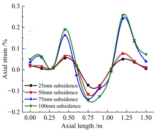
Figure 12. Axial Strain Curves at Pipe Crown During Different Landslide Stages.

4. Multifaceted Numerical Simulation Model

4.1. Soil Spring-Based Pipe–Soil Coupling Model

4.1.1. Soil Spring Constitutive Model

The core concept of the finite element simulation model based on soil springs is to simplify the soil constraint into nonlinear soil springs in the lateral, axial, and vertical directions. The nonlinear soil springs include two main parameters: the ultimate resistance and the yield displacement, as shown in Figure 13. The ALA-ASCE pipeline design guidelines provide the calculation methods for the soil springs per unit length of pipe in three directions [14]. P_u, T_u, Q_u, and Q_d represent the ultimate resistances of the lateral, axial, vertical upward, and vertical downward soil springs, respectively, while Δp, Δt, Δq_u, and Δq_d are the corresponding yield displacements. It can be seen that the soil springs in the lateral and axial directions exhibit symmetry. However, since pipelines are generally buried at shallow depths and the foundation depth is much greater than the burial depth, the ultimate resistance of the vertical upward soil spring Q_u is much smaller than that of the vertical downward soil spring Q_d. The main governing equations for calculating the ultimate resistance are as follows, while the required parameters and empirical values of soil yield displacement can be found in [14].

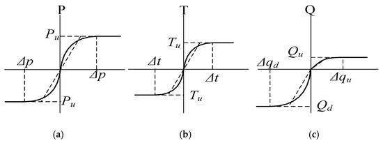
Figure 13. Schematic diagram of the soil spring constitutive model. (a) lateral direction, (b) axial direction, (c) vertical direction.

Lateral ultimate soil resistance calculation formula:

$$p_u=N_{ch}cD+N_{qh}\overline{\gamma }HD$$

(3)

In the equation, P_u denotes the horizontal ultimate soil resistance, kN/m; N_ch denotes the calculation parameter related to soil cohesion; N_qh denotes the calculation parameter related to the soil internal friction angle; c denotes the soil cohesion, kPa; D denotes the pipe diameter, m; $\overline{\gamma }$ denotes the effective unit weight of the soil, kN/m³; and H denotes the burial depth of the pipe center, m.

Axial ultimate soil resistance calculation equation:

$$T_u=\pi D\alpha c+\pi DH\overline{\gamma }{\displaystyle \frac{1+K_0}{2}}\tan \delta$$

(4)

In the equation, T_u denotes the axial ultimate soil resistance, kN/m; $\alpha$ denotes the soil cohesion coefficient; K₀ denotes the coefficient of earth pressure at rest; and $\delta$ denotes the pipe–soil interface friction angle, °.

Vertical upward ultimate soil resistance calculation equation:

$$Q_u=N_{cv}cD+N_{\mathrm{qv}}\overline{\gamma }HD$$

(5)

In the equation, Q_u denotes the vertical upward ultimate soil resistance, kN/m; N_cv denotes the calculation parameter related to soil cohesion; and N_qv denotes the calculation parameter related to the soil internal friction angle.

Vertical downward ultimate soil resistance calculation equation:

$$Q_d=N_{c}cD+N_q\overline{\gamma }HD+N_{\gamma }\gamma {\displaystyle \frac{D^2}{2}}$$

(6)

In the equation, Q_d denotes the vertical downward ultimate soil resistance, kN/m; N_c, N_q, and N_γ represent the bearing capacity factors; and γ denotes the total unit weight of soil, kN/m³.

4.1.2. Introduction of the Finite Element Model

In ABAQUS 2022, the stiffness properties of these springs in all three directions are implemented using PSI (Pipe–Soil Interaction) elements. The force-displacement relationship for each spring follows an ideal elastic-plastic curve. The calculated force-displacement values were input into the ABAQUS 2022-specific INP file to define the PSI elements. The pipeline is simulated using PIPE31 elements, a specialized beam-type element in ABAQUS/CAE specifically designed for tubular structures. The pipeline model has a length of 150 cm, consistent with the physical test model, with pipe nodes uniformly spaced at 1 cm intervals and corresponding soil nodes aligned accordingly. The peak soil resistance of the soil springs in all three directions can be calculated based on soil parameters and pipeline state parameters (diameter, burial depth) using the formulas provided in Section 4.1.1, while the soil yield displacement can be obtained by consulting Reference [14]. Figure 14 shows the schematic diagram of the PSI element.

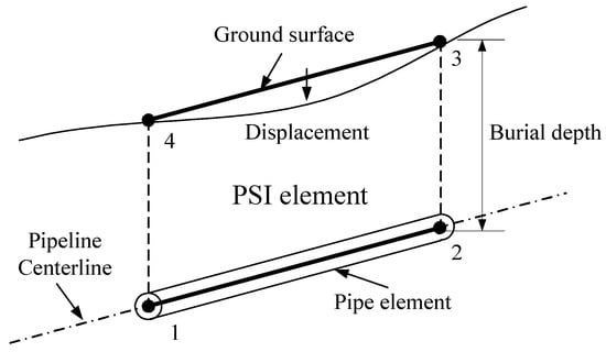
Figure 14. Schematic Diagram of PSI Element.

For three types of geohazard-induced pipe–soil interactions, different displacements are applied to the soil nodes, while translational degrees of freedom are constrained at both ends of the pipeline. In the fault displacement model, a 100 mm vertical upward displacement is applied to the soil nodes on the right side within a 500 mm zone. In the soil settlement model, continuous settlement displacement is applied to the surface soil nodes in the central 500 mm settlement area. In the lateral landslide model, a 100 mm horizontal displacement is applied to the soil nodes within the central landslide zone. These displacements are transferred to the pipe elements through the PSI units, thereby simulating the mechanical state of the pipeline under different geohazard-induced displacement loads. Figure 15 illustrates the schematic diagram of the finite element model.

Figure 15. Schematic Diagram of the Finite Element Model Based on PSI Element.

4.2. Traditional FEM Pipe–Soil Coupling Model

4.2.1. FEM Method

The core concept of the FEM is to systematically discretize the continuous pipeline and the surrounding soil medium into a series of simple elements connected by nodes. The fundamental unknowns directly solved in FEM are the nodal displacements. Once the displacements of all nodes are obtained, the shape functions of the elements are used, together with differential operations, to interpolate and calculate the strain at any point within each element. After obtaining the strain field, the corresponding stress at each point can be derived from the calculated strain by introducing a constitutive model that describes the material’s mechanical behavior. The explicit calculation method adopted in this study has its dynamic equilibrium equation expressed as shown in Equation (7):

$$M\stackrel{··}{{\displaystyle u}}+C\stackrel{·}{{\displaystyle u}}+Ku=P(t)$$

(7)

In the equation, M denotes the mass matrix, kg; C denotes the system damping matrix, N·s/m; K denotes the system stiffness matrix, N/m; $\stackrel{··}{u}$ denotes the nodal acceleration, m/s²; $\stackrel{·}{u}$ denotes the nodal velocity, m/s; u is the noadal displacemnet, m; and P(t) denotes the time-dependent external force vector, N.

The integration of acceleration over time is carried out using the central difference method, that is, the nodal velocity at the midpoint of the current increment step is equal to the velocity change obtained in this step plus the nodal velocity at the midpoint of the previous increment step.

$$\stackrel{·}{{\displaystyle u}}{|}_{(t+{\displaystyle \frac{△t}{2}})}=\stackrel{·}{{\displaystyle u}}{|}_{(t-{\displaystyle \frac{△t}{2}})}+{\displaystyle \frac{(△t{|}_{(t+△t)}+△t{|}_{(t)})}{2}}\stackrel{··}{{\displaystyle u}}{|}_{(t)}$$

(8)

In the equation, $\stackrel{·}{{\displaystyle u}}{|}_{(t+{\displaystyle \frac{△t}{2}})}$ denotes the nodal velocity at the midpoint of the current increment step, m/s; $\stackrel{·}{{\displaystyle u}}{|}_{(t-{\displaystyle \frac{△t}{2}})}$ denotes the nodal velocity at the midpoint of the previous increment step, m/s; ${\displaystyle \frac{(△t{|}_{(t+△t)}+△t{|}_{(t)})}{2}}$ represents the arithmetic average of the time step at instant t and the next time step, s; and $\stackrel{··}{{\displaystyle u}}{|}_{(t)}$ denotes the nodal acceleration at time, m/s².

The integration of velocity over time, combined with the displacement at the beginning of the increment step, yields the displacement at the end of the increment step.

$$u{|}_{(t+△t)}=u{|}_{(t)}+△t{|}_{(t+△t)}\stackrel{·}{{\displaystyle u}}{|}_{(t+{\displaystyle \frac{△t}{2}})}$$

(9)

In the equation, $u{|}_{(t+△t)}$ denotes the displacement at the end of the increment step, m, and $u{|}_{(t)}$ denotes the displacement at the beginning of the increment step, m.

4.2.2. Introduction of the Finite Element Model

Nonlinear finite element software ABAQUS 2022 was used to establish pipe–soil coupling models for fault displacement, ground settlement, and landslide scenarios. The model dimensions and pipeline parameters were kept consistent with the experimental setup. The soil was modeled using C3D8R (8-node hexahedral linear reduced integration element) elements, while the pipeline was modeled with S4R shell elements. The pipe–soil interface was characterized using “Surface to Surface” contact, with hard contact in the normal direction and a penalty function in the tangential direction, where the friction coefficient was set to 0.38. The friction coefficient is taken as the tangent of the pipe–soil interface friction angle. The soil properties were described using the Mohr-Coulomb constitutive model [15]. To ensure solution accuracy, the soil mesh near the pipe–soil interface was refined, while coarser meshes were used for soil regions farther from the interface. The model consists of two analysis steps: the first step applies gravitational loading, while the second step imposes soil displacement. It should be noted that for the fixed soil section, all surfaces except the top surface are constrained in the normal direction, while the movable soil section is subjected to the prescribed displacement pattern. The pipe-soil interaction models under different geohazard conditions are illustrated in Figure 16, Figure 17 and Figure 18.

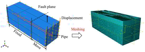
Figure 16. Pipe–Soil Coupling Model Under Fault Displacement (Traditional FEM).

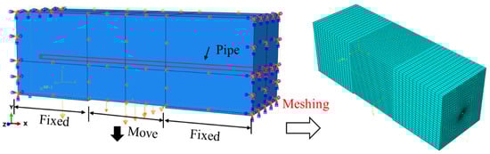
Figure 17. Pipe–Soil Coupling Model Under Settlement Displacement (Traditional FEM).

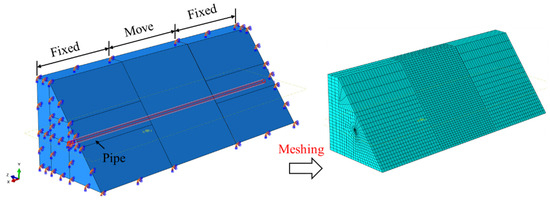
Figure 18. Pipe–Soil Coupling Model Under Landslide Displacement (Traditional FEM).

4.3. SPH-FEM Pipe–Soil Coupling Mode

4.3.1. SPH Method

The SPH method is a mesh-free, purely Lagrangian approach based on interpolation theory [16]. Compared with mesh-based methods, the main advantage of applying SPH to solid mechanics is its ability to handle larger local deformations. The core idea is to discretize the computational domain into a certain number of particles, each having a specific mass and volume, as well as physical properties such as density, velocity, acceleration, and stress. By solving for the discrete particles individually, the overall information of the continuum can be obtained [17]. In ABAQUS 2022, particles can be converted from C3D8R elements. After the particle conversion, the state information associated with the original elements (such as stress, strain, and displacement) is transferred to the generated particles. The activated particles then interact with adjacent non-particle meshes in the SPH formulation. Gravity loads, contact interactions, initial conditions, and outputs associated with the parent elements are transferred to the generated particles during the conversion. A set of built-in special algorithms in ABAQUS 2022 ensures a smooth transition between the two modeling approaches as far as possible. The contact surface of the SPH–FEM coupling is shown in Figure 19.

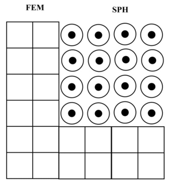
Figure 19. FEM-SPH coupling diagram.

In the SPH solution process, within the domain $\Omega$, any continuous field macroscopic variable function F(x) in space is expressed in an integral form through a smoothed interpolation approximation [18]:

$$F\left(x\right)={\displaystyle {\int }_{\Omega }F\left(x^{\prime }\right)}\delta \left(x-x^{\prime }\right)d{x}^{\prime }$$

(10)

In the equation, F(x) denotes a macroscopic variable function of the continuous field to be solved, such as displacement or stress; $\Omega$ is the domain of the variable; and $\delta \left(x-x^{\prime }\right)$ is the Dirac delta function.

By replacing the Dirac delta function with an interpolation kernel function $W=W\left(x-x^{\prime },\mathrm{h}\right)$, the kernel approximation expression of the SPH method is obtained.

$$⟨F\left(x\right)⟩={\displaystyle \underset{\Omega }{\int }F\left(x^{\prime }\right)W\left(x-x^{\prime },h\right)}d{x}^{\prime }$$

(11)

In the equation, $⟨F\left(x\right)⟩$ is the smoothed estimate; h is the smoothing length, i.e., the influence radius of the interpolation kernel function, which determines how many particles contribute to the interpolation at a given point.

4.3.2. Introduction of the Finite Element Model

The soil domain was initially meshed with C3D8R hexahedral elements, which were subsequently converted to PC3D particles using cubic kernel functions, while the pipeline was modeled with S4R shell elements. Unlike traditional FEM approaches, SPH particles cannot directly accommodate boundary conditions and require constraint through contact interactions. Thus, a bounding box with constrained boundaries was implemented to confine the particle domain. Particle mass and volume were automatically calculated based on their parent elements, with SPH smoothing lengths and computational domains determined through the same conversion process. Initial conditions (stress/strain fields, displacements, material properties), gravity loads, and interaction definitions from the parent elements were transferred to the particles, whereas nodal boundary conditions applied to the parent elements were not inherited by the SPH particles. The SPH method employs a meshless Lagrangian formulation to represent soil as a collection of mass-smoothed particles, eliminating mesh distortion issues inherent in traditional Lagrangian analyses during large soil deformations. Soil-pipeline coupling was achieved through Lagrangian contact definitions between SPH particles and shell elements, with contact behavior consistent with traditional FEM settings. The model dimensions and pipe–soil interaction mechanisms for all three geohazard scenarios maintained consistency with the physical test setup, including identical pipe material properties, soil constitutive models, and contact definitions as in traditional FEM. However, soil displacements were applied to the external bounding box or base plate rather than directly to SPH particles, as particle-based systems cannot receive direct displacement loading. The pipe-soil interaction models under different geohazard conditions are illustrated in Figure 20, Figure 21 and Figure 22.

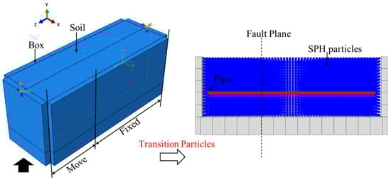
Figure 20. Pipe–Soil Coupling Model Under Fault Displacement (SPH-FEM).

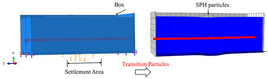
Figure 21. Pipe–Soil Coupling Model Under Settlement Displacement SPH-FEM).

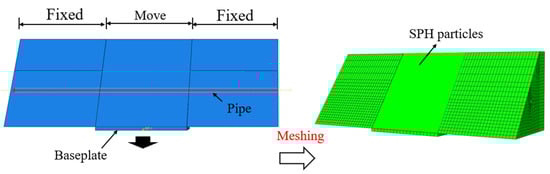
Figure 22. Pipe–Soil Coupling Model Under Landslide Displacement (SPH-FEM).

5. Analysis of Numerical Simulation and Experimental Results

5.1. Fault Action

To verify the accuracy of different pipe–soil coupling numerical models in simulating fault-induced soil displacement, a comparative analysis was conducted between small-scale laboratory fault test results and three numerical approaches: the nonlinear soil spring model, traditional FEM model, and SPH-FEM coupled model. Figure 23 presents the deformation contour plots obtained from these distinct finite element modeling methodologies.

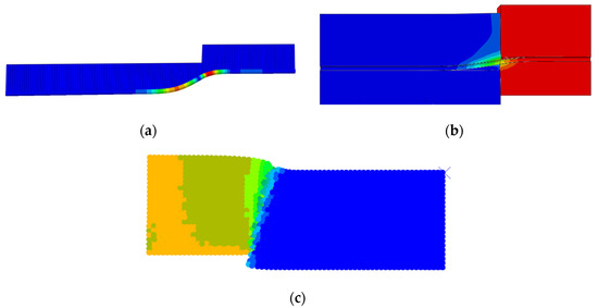
Figure 23. Deformation Contours of Different Finite Element Models Under Fault Displacement: (a) Model based on soil springs; (b) Traditional FEM model; (c) SPH-FEM model.

The comparison curves between numerical simulation results and experimental measurements of axial strain at the pipe crown under different fault displacements are shown in Figure 24. The distribution trends of axial strain obtained from the three numerical models (nonlinear soil spring, traditional FEM, and SPH-FEM) are similar to those observed in small-scale laboratory tests. Strain concentrations primarily occur on both sides of the fault plane, with the maximum axial tensile and compressive strains located near monitoring points S8 and S6, respectively. However, significant differences exist in the numerical values predicted by the three models. Using the experimental measurements as a benchmark, at fault displacements of 25 mm and 50 mm, the traditional FEM model results are slightly higher than the experimental values, with relative errors of 21.14% and 28.07% for the maximum axial strains, respectively. The SPH-FEM model results are generally lower than the experimental values, with larger relative errors of 32.86% and 44.16%. The soil spring model significantly overestimates the strains compared to the experimental measurements. At fault displacements of 75 mm and 100 mm, the traditional FEM model overestimates the axial strain on the right (tensile) side of the pipe but slightly underestimates the strain on the left (compressive) side, with relative errors of 26.33% and 15.32% for the maximum axial strains. The SPH-FEM model slightly underestimates the axial strain on the tensile side, with relative errors of 22.95% and 18.62%. The soil spring model still exhibits large discrepancies, with relative errors exceeding 50% compared to the experimental measurements.

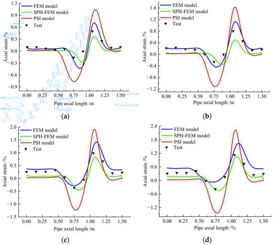
Figure 24. Axial Strain of Pipeline Under Different Fault Displacements: (a) 25 mm displacement; (b) 50 mm displacement; (c) 75 mm displacement; (d) 100 mm displacement.

The relative errors between computational results from both the traditional FEM model and SPH-FEM coupled pipe–soil model and experimental measurements remain within generally acceptable engineering tolerances. Under smaller fault displacements, the SPH-FEM model demonstrates deviations exceeding 30% relative to experimental values, showing inferior accuracy compared to the traditional FEM model. However, as fault displacements increase, the relative error between SPH-FEM simulation results and measured values decreases. Overall, the traditional FEM pipe–soil model yields more accurate computational results. In terms of computational efficiency, the SPH-FEM coupled model requires the longest calculation time, exceeding six times that of the traditional FEM model. While the SPH particle-based soil model can effectively simulate soil fracturing, it fails to demonstrate significant advantages for small-scale test conditions. The soil spring model exhibits the shortest computation time, yet its results show marked discrepancies with experimental values, rendering it unsuitable for localized pipeline simulations.

5.2. Settlement Action

Figure 25 displays the deformation contour plots of different finite element models under ground settlement conditions. The computational results of three pipe–soil coupling models were compared with experimental data to evaluate their accuracy in simulating settlement-induced soil displacement. Figure 26 shows the comparison curves between numerical simulations and experimental measurements of axial strain at the pipe crown under different settlement magnitudes. The traditional FEM model generally overestimated strain values compared to experimental results, while the SPH-FEM model tended to underestimate them. At 25 mm maximum settlement, the relative errors of the FEM model and SPH-FEM model compared to experimental results were 13.82% and 39.86%, respectively. At 50 mm settlement, these errors were 12.51% and 32.77%. The soil spring model showed significant discrepancies, with errors exceeding 50% relative to experimental measurements. The FEM model demonstrated the highest accuracy, while the SPH-FEM model’s underestimation and larger errors were attributed to its limitations in handling small deformations at this scale. Additionally, the SPH-FEM model exhibited substantially lower computational efficiency compared to traditional mesh-based approaches.

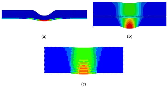
Figure 25. Deformation Contours of Different Finite Element Models Under Settlement Displacement: (a) Model based on soil springs; (b) Traditional FEM model; (c) SPH-FEM model.

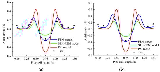
Figure 26. Axial Strain of Pipeline Under Different Settlement Displacements: (a) 25 mm settlement; (b) 50 mm settlement.

5.3. Landslide Action

Figure 27 shows the deformation contour plots of different finite element models under landslide conditions. It can be seen that the soil displacements of both the soil spring model and the traditional FEM model are continuous, while the SPH-FEM model shows obvious discontinuous soil displacement, which is consistent with the soil behavior observed in the experiments.

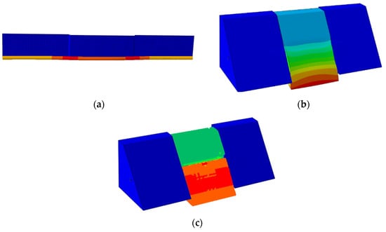
Figure 27. Deformation Contours of Different Finite Element Models Under Landslide Displacement: (a) Model based on soil springs; (b) Traditional FEM model; (c) SPH-FEM model.

The computational results of three types of pipe–soil coupling numerical models under landslide conditions were compared with experimental measurements. The comparison curves between numerically calculated and experimentally measured axial strains at the pipe crown under different landslide displacements are shown in Figure 28. All three models predicted similar axial strain distribution patterns on the landslide-facing pipe surface, with maximum compressive strain occurring at the pipe mid-span and peak tensile strain developing near the boundary outside the landslide zone. However, significant numerical discrepancies were observed. For the first three loading cases, both the traditional FEM model and SPH-FEM model produced slightly higher results compared to experimental measurements. The relative errors between the traditional FEM model simulations and experimental measurements were 24.24%, 17.12%, and 30.75% for the three landslide displacement cases, while the SPH-FEM model showed relative errors of 42.04%, 44.29%, and 44.52%. The traditional FEM model had smaller calculation errors than the SPH-FEM model. When the landslide displacement reached 100 mm, the traditional FEM model calculation results increased significantly, while the SPH-FEM model axial strain calculation results decreased compared to the previous stage. Their relative errors compared to experimental measurements were 98.95% and 25.95%, respectively. The SPH-FEM model results showed reduced relative errors, whereas the traditional FEM model results exhibited a sharp error increase. This occurred because, under large landslide displacements, severe mesh distortion occurred around the pipe in the soil domain, and the solid elements could not simulate soil fracturing, leading to abnormal calculation results in the solid soil model. The advantage of the meshless SPH method lies in its ability to simulate soil fracturing during landslides under large deformation conditions. When landslide displacements are large and soil fracturing is severe, the soil’s force on the pipeline weakens, causing the SPH-FEM model calculation results to gradually decrease. This trend aligns with the experimental strain measurements. However, the SPH-FEM method has lower computational efficiency and is less accurate than the traditional FEM model for small soil deformations.

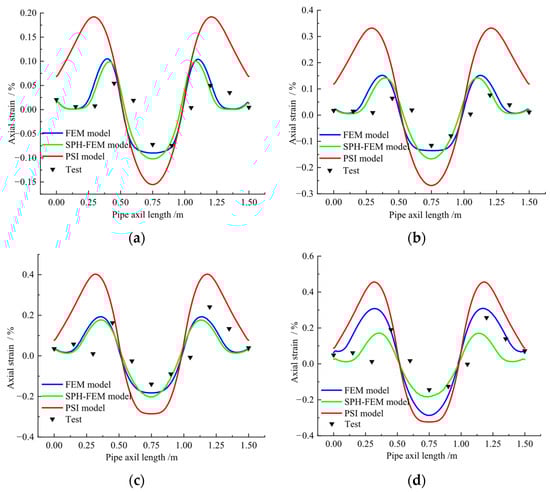
Figure 28. Axial Strain of Pipeline Under Different Landslide Displacements: (a) 25 mm leading edge displacement; (b) 50 mm leading edge displacement; (c) 75 mm leading edge displacement; (d) 100 mm leading edge displacement.

6. Conclusions

This study conducted physical scale-model tests of pipe–soil interaction under three geohazard scenarios—fault displacement, ground subsidence, and landslide—to characterize soil deformation patterns and pipeline mechanical responses. Numerical back-analysis of these experimental cases was performed using three distinct modeling approaches: the soil spring-based numerical model, traditional FEM model, and SPH-FEM coupling model. Through systematic comparison, the applicability of each modeling technique for different geohazard types was evaluated, yielding the following key findings:

(1) The nonlinear soil spring model, based on the ALA-ASCE standard, simplifies pipe–soil interaction into spring elements and offers the highest computational efficiency. However, its simulation results show significant discrepancies with experimental data, with errors typically exceeding 50%. It is mainly suitable for rapid engineering assessments. These findings also indicate that the current accuracy of soil spring models requires improvement.

(2) The traditional FEM model demonstrates higher accuracy when soil displacement is small, with relative errors generally below 30% compared to experimental measurements. It performs well under reverse fault and soil settlement conditions, closely matching experimental results. However, when soil deformation is large, mesh distortion occurs, leading to a significant increase in error.

(3) The SPH-FEM coupled pipe–soil model demonstrates exceptional performance under large-displacement conditions. By integrating meshless particle methods with finite element coupling, it effectively simulates soil behavior during large deformations and accurately captures discontinuous features such as soil flow and cracking.

(4) Comparative analysis reveals that the soil spring-based numerical model is suitable for rapid engineering assessments; the traditional FEM model demonstrates superior performance in handling small soil deformations by balancing computational accuracy and efficiency; while the SPH-FEM coupling model, leveraging its meshless characteristics, excels in addressing large soil deformation problems. The novelty of this study lies in its systematic comparison of the applicability of these numerical simulation models, providing valuable references for researchers in related fields.

References

- Kong, T.W.; Liu, X.B.; Huang, W.; Liu, C.Q.; Zhang, D.; Zhang, J.; Zhang, H. Strain response study of CFRP pre-reinforced pipelines under reverse fault displacement. China Pet. Pet. Mach. 2023, 51, 127–135. [Google Scholar]
- Liang, Y.; Tu, R.; Zhang, H.; Liu, C.; Fu, G.; Qiu, R.; Liao, Q.; Xu, N. Role of oil and gas pipelines in the construction of a new energy system with multi-energy integration. Oil Gas Storage Transp. 2025, 44, 361–378. [Google Scholar] [CrossRef]
- Zhang, H. Analysis of Pipeline Stress State and Risk Assessment Under Slope Conditions. Master’s Thesis, China University of Mining and Technology, Beijing, China, 2024. [Google Scholar]
- Lim, Y.M.; Kim, M.K.; Kim, T.W.; Jang, J. The behavior analysis of buried pipeline: Considering longitudinal permanent ground deformation. In Pipelines 2001: Advances in Pipelines Engineering and Construction; American Society of Civil Engineers: Reston, VA, USA, 2001; pp. 1–11. [Google Scholar]
- Takada, S.; Hassani, N.; Fukuda, K. A new proposal for simplified design of buried steel pipes crossing active faults. Earthq. Eng. Struct. Dyn. 2001, 30, 1243–1257. [Google Scholar] [CrossRef]
- Xie, X.; Symans, M.D.; O’Rourke, M.J.; Abdoun, T.H.; O’Rourke, T.D.; Palmer, M.C.; Stewart, H.E. Numerical modeling of buried HDPE pipelines subjected to normal faulting: A case study. Earthq. Spectra 2013, 29, 609–632. [Google Scholar] [CrossRef]
- Zhang, F.; Liu, M.; Wang, Y.Y.; Yu, Z.; Tong, L. Strain demand in areas of mine subsidence. In Proceedings of the 2012 International Pipeline Conference, Calgary, AB, Canada, 24–28 September 2012; American Society of Mechanical Engineers: New York, NY, USA, 2012; pp. 391–401. [Google Scholar]
- Ji, B.L. Research on Digital Twin Technology for Pipeline Structures in Geological Hazard Zones. Master’s thesis, China University of Petroleum (Beijing), Beijing, China, 2022. [Google Scholar]
- Zhao, J.; Liu, H.; Zhang, X. Numerical analysis of pipeline responses to ground subsidence. Tunn. Undergr. Space Technol. 2014, 40, 1–8. [Google Scholar]
- Tang, L. Failure mechanism analysis of buried pipelines subjected to slope movement: Numerical modeling and parametric study. Eng. Fail. Anal. 2020, 111, 104453. [Google Scholar]
- Karamitros, D.K.; Bouckovalas, G.D.; Kouretzis, G.P. Numerical simulation of fault-pipeline interaction and its effects on design. Tunn. Undergr. Space Technol. 2017, 70, 1–9. [Google Scholar]
- Zhang, J.; Huang, S.; Wang, H.; He, J.; Zhao, H.; Zhou, B.; Liu, J. Interaction of pipelines with landslides: Analysis of mechanical properties at different strengths. Vibroeng. Procedia 2024, 57, 59–65. [Google Scholar] [CrossRef]
- GB/T 50123; Standard for Geotechnical Testing Method. Ministry of Housing and the People’s Republic of China: Beijing, China, 2019.
- American Lifelines Alliance (ALA). Guidelines for the Design of Buried Steel Pipe; American Society of Civil Engineers: Reston, VA, USA, 2001. [Google Scholar]
- Fei, K.; Zhang, J. Application of ABAQUS in Geotechnical Engineering; China Water & Power Press: Beijing, China, 2013. [Google Scholar]
- Wang, H.B.; Yan, F.; Zhang, L.W.; Zhang, W.; Li, X.M.; Wang, S.Q.; Wang, S. Mechanism and flow process of debris avalanche in mining waste dump based on improved SPH simulation. Eng. Fail. Anal. 2022, 138, 106345. [Google Scholar] [CrossRef]
- Feng, D.; Imin, R. A kernel derivative free SPH method. Results Appl. Math. 2023, 17, 100355. [Google Scholar] [CrossRef]
- Sigalotti, L.D.G.; Klapp, J.; Gesteira, M.G. The mathematics of smoothed particle hydrodynamics (SPH) consistency. Front. Appl. Math. Stat. 2021, 7, 797455. [Google Scholar] [CrossRef]
Disclaimer/Publisher’s Note: The statements, opinions and data contained in all publications are solely those of the individual author(s) and contributor(s) and not of MDPI and/or the editor(s). MDPI and/or the editor(s) disclaim responsibility for any injury to people or property resulting from any ideas, methods, instructions or products referred to in the content. |
© 2025 by the authors. Licensee MDPI, Basel, Switzerland. This article is an open access article distributed under the terms and conditions of the Creative Commons Attribution (CC BY) license (https://creativecommons.org/licenses/by/4.0/).