Coupled LEM–CZM Numerical Framework for Landslide Simulation and Its Application to Geotechnical Design

Abstract

To realistically simulate the entire slip-surface process from crack initiation to run-out, we couple the simplified Bishop method (LEM) with zero-thickness cohesive elements (CZM): LEM first pinpoints the critical slip circle, then CZM tracks interface opening, progressive damage, and sliding along that exact surface. Benchmarked against ACADS EX11, the framework reproduces the classical factor of safety while delivering the post-failure displacements, energy dissipation, and crack paths that LEM or traditional FEM cannot capture, offering a practical tool for landslide-prone slope design.

1. Introduction

Landslides are among the most destructive geological hazards, often evolving through distinct phases: initial crack formation, progressive structural failure, rapid sliding, and eventual impact. Accurately predicting both the location of potential failure surfaces and the subsequent rupture behavior of the sliding mass is essential for understanding landslide mechanisms and for developing effective mitigation strategies. Generally speaking, there are three main types of numerical simulation of slopes: empirical and analytical methods, limit equilibrium, and continuous discrete numerical methods.

Empirical rating systems such as rock mass rating (RMR) and slope mass rating (SMR) [1,2] and landslide-inventory susceptibility models [3] deliver fast regional hazard zoning. GIS-based landslide assessment now couples empirical rock-mass classifications with spatial-statistical tools to generate regional hazard maps in minutes. High-resolution DEMs, UAV-LiDAR-derived discontinuity orientations, and monsoon rainfall rasters are imported into ArcGIS Pro 3.0 where the RMR/SMR check-lists are coded as reusable Python 2020 raster functions; the resulting 0–100 grids are re-classified into five susceptibility zones that correctly predict > 80% of the post-mapping failures along NH-44 in the Kashmir Himalaya, giving AUC = 0.78 [4]. The same workflow has been ported to inventory-based models: logistic regression, weights-of-evidence, and artificial neural networks executed inside GIS statistically relate past slide polygons to SMR together with slope, lithology, and land-cover covariates. In Chandpur, Uttarakhand, adding the continuous SMR grid as a predictor raised the success rate from 71% to 84% and concentrated the “very-high” class around the main town, demonstrating that hybrid GIS platforms merge the speed of empirical ratings with the adaptability of data-driven susceptibility mapping [5]. Analytical upper-bound and energy-based limit analyses [6,7] provide rapid stability estimates for simple geometries, but their accuracy drops significantly under complex hydrogeological conditions. These methods remain correlative and cannot predict crack paths or time-dependent deformation.

Another widely used method is the limit equilibrium method (LEM). which evaluates slope safety by dividing the potential sliding mass into slices and enforcing force and moment equilibrium [8,9]. While LEM is computationally efficient and widely adopted for identifying critical slip surfaces, it is fundamentally limited by its assumptions: it treats the sliding mass as a rigid body, neglects material deformation and post-failure behavior, and cannot capture fracture propagation or progressive failure mechanisms [8,9,10]. Consequently, LEM provides a static safety factor but offers no insight into the dynamic evolution of slope failure.

With the development of numerical computation, a lot of new methods are employed to simulate the failure of slopes. The first type is used for the evaluation of the safety of slope. The strength reduction method based on FEM and FDM is widely used and accepted as the alternative of LEM. A lot of commercial codes like FLAC3D GeoStudio have integrated this method. Another type is for the evaluation of the failure mode of landslide.

Considering the large deformation after failure, almost any discontinuous numerical methods, such as discrete element method (DEM) [11], cohesive zone model (CZM), finite element method (FDEM) [12], SPH-based large deformation model [13], Smoothed Particle Hydrodynamics (SPH), Material Point Method (MPM), peridynamics, and extended finite element method (XFEM), can be used for failure simulation.

The empirical and analytical method is suitable for limited situations like the regional evaluation or simple geometry. The LEM can only evaluate the safety factor and cannot simulate the deformation of the slope. The continuous and discontinuous numerical method can give accuracy to the simulation. But the failure of the slope involved the localization and the thin shear band is generated and the parameter on the shear band is weaker than the other region. In terms of modeling the phenomena of slope, many complex techniques should be used. This manuscript LEM–CZM method employs the LEM to compute the safety factor and shear band, and CZM to simulate the failure mode of the slope, providing a simple but effective solution for this problem to evaluate the safety factor and failure mode.

2. Method

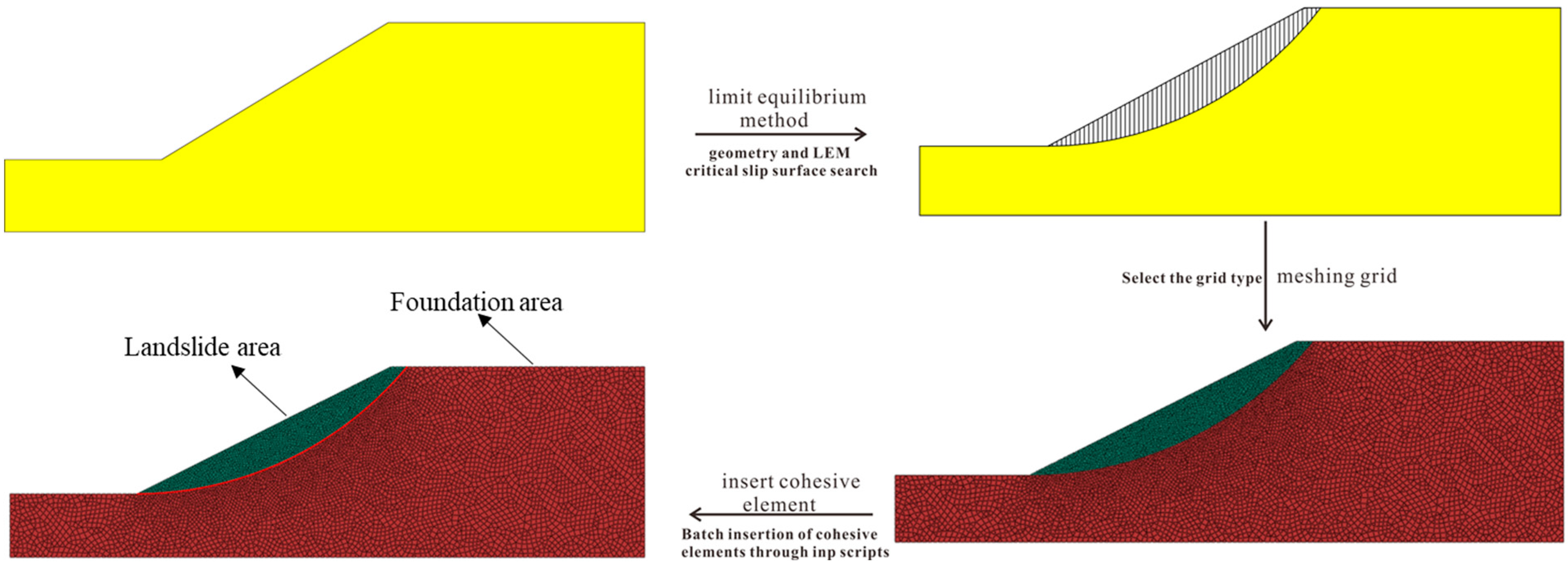
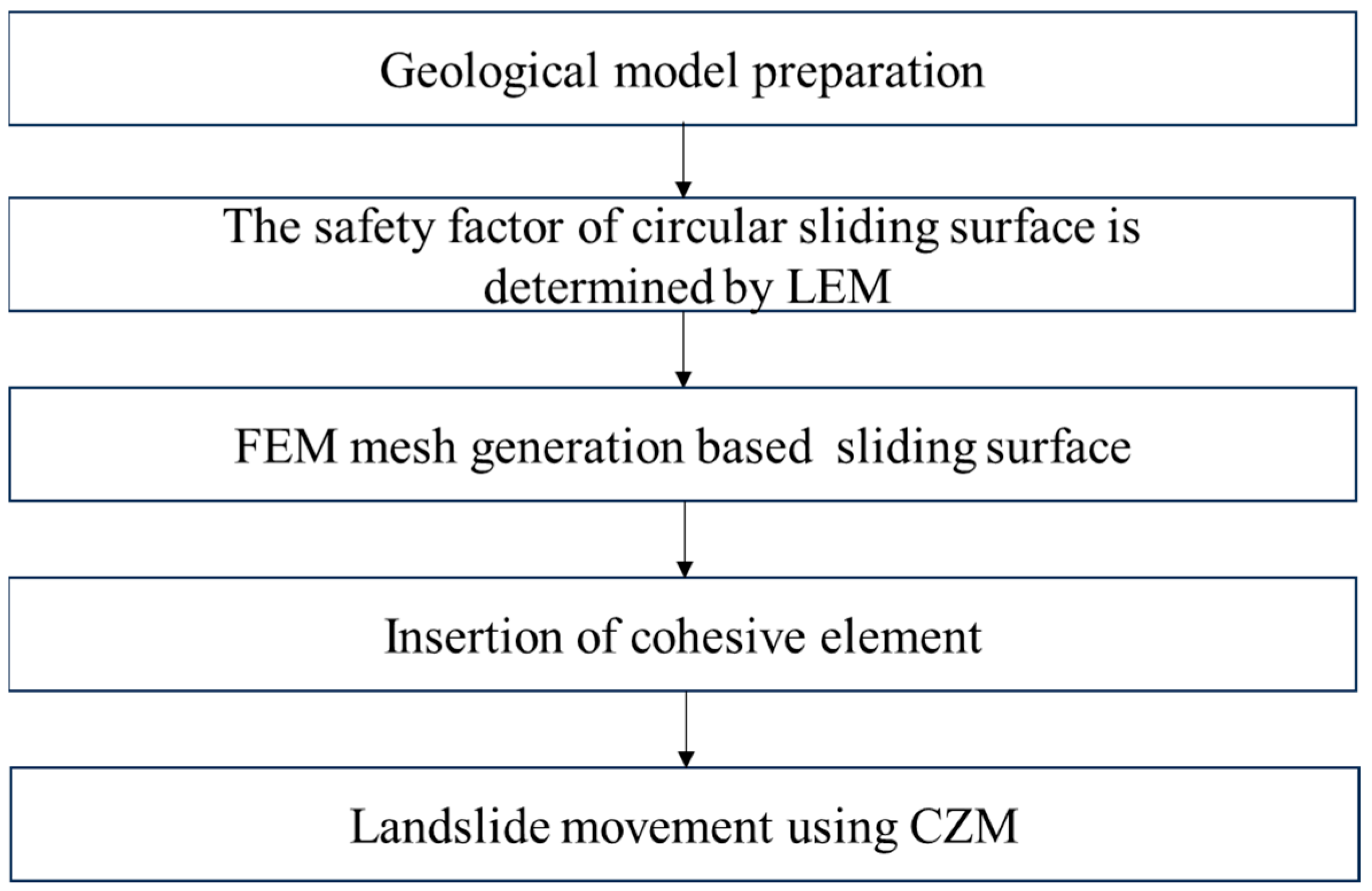
This study proposes a coupled LEM–CZM framework that synergizes the strengths of both methods. This coupling enables a continuous, physically realistic simulation of landslide evolution—from initial instability to final collapse—while preserving computational efficiency. The framework is validated using the ACADS benchmark problem EX11, demonstrating its superiority over standalone LEM (which ignores post-failure kinematics) or CZM (which struggles with arbitrary crack paths). By integrating classical slope stability theory with modern fracture mechanics, the proposed LEM–CZM framework serves as a complementary rather than alternative tool to conventional factor-of-safety (Fs) approaches. While Fs aims to prevent failure by ensuring a prescribed safety margin, the coupled model quantifies post-failure kinematics (run-out distance, sliding velocity, and energy dissipation) once the Fs is exceeded. It allows engineers to (i) evaluate how far and how fast a potential slide will travel, (ii) compare the efficiency of mitigation options (e.g., rock-bolt length, geogrid stiffness, or catch-bench width) in reducing these post-failure metrics, and (iii) optimize the location and capacity of retaining structures or deflection dams based on predicted displacement fields rather than on Fs alone. Consequently, the framework provides an additional design criterion—performance-based landslide mitigation—that works alongside traditional Fs calculations to achieve more economical and resilient slope stabilization solutions in landslide-prone regions [14,15]. Its modular structure further allows extensions to 3D geometries, non-circular slip surfaces, and hydro-mechanical coupling. The specific flow chart is shown in Figure 1.

Figure 1. Flow chart of LEM–CZM simulation.

2.1. Limit Equilibrium Analysis

The limit equilibrium method (LEM) is widely used in slope stability analysis and calculation. The theoretical basis of this method is the Mohr-Coulomb strength criterion [8,15]. A commonly used form of the LEM is the strip method, in which the soil mass is divided into vertical strips, and the equilibrium conditions of each strip are analyzed to evaluate overall slope stability. This approach introduces significant mathematical indeterminacy—for n slices, there are 5n−2 unknowns (normal forces, shear forces, line of thrust locations, and interslice forces) but only 3n equilibrium equations (force and moment balance)—creating a statically indeterminate system. However, several limitations arise when using the strip method. With more slices employed, the degree of static indeterminacy rises, thereby amplifying the need for additional kinematic or constitutive assumptions to achieve a solution. To address this, simplifying assumptions about interslice force directions must be introduced. The Bishop method assumes horizontal interslice forces (neglecting shear forces), reducing unknowns while maintaining good accuracy for circular slip surfaces. More advanced methods like Morgenstern–Price specify a functional relationship (e.g., half-sine function) between the inclination and magnitude of interslice forces, providing additional equations to achieve static determinacy [16].

The assumptions for force distribution typically follow two fundamental principles: (1) there is a maximum shear capacity for each soil strip, and the shear stresses on both sides must not exceed this limit; and (2) only shear and compressive stresses are allowed on the contact surface between strips, with tensile stress being neglected [17]. Based on the strip method framework, a variety of classical approaches have been developed, including the Swedish circle method, the simplified Bishop method, and the Janbu method [18]. Among these, the simplified Bishop method is one of the most widely used techniques for slope stability analysis [19,20,21,22,23]. The algorithm adopted in this study is also based on this method.

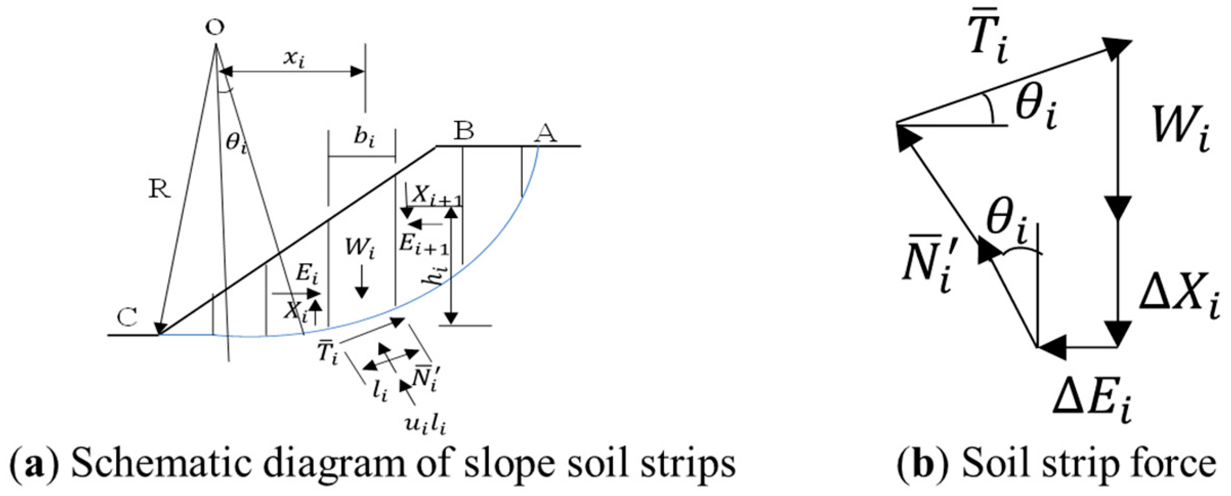
The Bishop strip method was proposed by British scientist Bishop [24]. This method assumes that the sliding surface is an arc with a center of O and a radius of R. It also takes into account the forces on the sides of the soil strips and assumes that all slices are assigned the same base-slice safety factor, which coincides with the overall average for the complete slip surface. This uniform FS is an inherent requirement of the limit equilibrium formulation, determined iteratively to satisfy global equilibrium conditions, rather than being an arithmetic average of individual strip safety factors. Bishop derived the formula using the effective stress method, and total stress analysis can also be used. The schematic diagram of the calculation principle is shown in Figure 2.

Figure 2. Bishop’s method of slices calculation diagram.

This takes a soil strip where $i{,\theta }_i$ is the inclination angle between the bottom and the horizontal plane, $\Delta X_i$ is the force difference in the horizontal soil strip around the soil strip I, and the forces on it include self-weight $W_i$, bottom tangential shear force ${\overline{T}}_i$, effective normal reaction force ${\overline{N}}_i^{\prime }$, and pore water pressure $u_i{l}_i$. Assume that the points of action of these forces are all at the midpoint of the bottom surface of the soil strip. In addition, normal force, cohesion c, and the shear forces on the two vertical faces of slice $i$ are included; vertical equilibrium of this slice gives

$$W_i+\Delta X_i-{\overline{T}}_{i}sin{\theta }_i-{{\overline{N}}_i}^{\prime }cos{\theta }_i-u_i{l}_{i}cos{\theta }_i=0,$$

(1)

Equivalent to

$${{\overline{N}}_i}^{\prime }cos{\theta }_i=W_i+\Delta X_i-{\overline{T}}_{i}sin{\theta }_i-u_i{b}_i,$$

(2)

where $b_i$ is the width of the bottom of $i$.

When the soil slope is not damaged, only a fraction of the slip-surface shear strength is mobilized. If expressed in terms of effective stress, the shear resistance mobilized along the slice base is

$${\overline{T}}_i={\displaystyle \frac{{\tau }_{fi}l}{F_s}}={\displaystyle \frac{c^{\prime }{l}_i}{F_s}}+{\displaystyle \frac{{{\overline{N}}_i}^{\prime }{tan\phi }^{\prime }}{F_s}},$$

(3)

where $c^{\prime }$ is the effective cohesion; ${\tau }_{fi}$ is the ultimate shear strength of the bottom; $l_i$ is the bottom arc length; ${tan\phi }^{\prime }$ is the effective internal friction coefficient; $F_s$ is the safety factor.

Substitute into formula (2), we can solve ${\overline{N}}_i^{\prime }$ and obtain the formula

$${{\overline{N}}_i}^{\prime }={\displaystyle \frac{1}{m_{\theta i}}}(W_i+\Delta X_i-u_i{b}_i-{\displaystyle \frac{c^{\prime }{l}_i}{F_s}}sin{\theta }_i),$$

(4)

where $m_{\theta i}$ is the Bishop correction factor.

In the formula

$$m_{\theta i}=cos{\theta }_i+{\displaystyle \frac{ {tan\phi }^{\prime }}{F_s}}sin{\theta }_i,$$

(5)

The moment equilibrium of the entire sliding soil around the center o is calculated. At this time, the moments of the side wall forces between adjacent soil strips cancel each other out, and the lines of action of ${\overline{N}}_i^{\prime }$ and $u_i{l}_i$ of each soil strip pass through the center of the circle, so we can obtain

$${\displaystyle \sum _i{W}_i{x}_i}-{\displaystyle \sum _i{\overline{T}}_i}R=0,$$

(6)

where $R$ is the radius of the slip surface arc.

Substitute Equation (4) into Equation (3) and then into the above equation. Since $x_i=Rsin{\theta }_i$, we obtain

$$F_s={\displaystyle \frac{\sum \frac{1}{m_{\theta i}}\left[c^{\prime }{b}_i+(W_i-u_i{b}_i+\Delta X_i){tan\phi }^{\prime }\right]}{\sum W_{i}sin{\theta }_i}},$$

(7)

This is Bishop’s general formula for calculating the safety factor of soil slopes, in which ${∆X}_i$ is still an unknown quantity. In order to obtain $F_s$, it is necessary to estimate the value of ${∆X}_i$, which can be solved by the method of successive approximation. The trial values of $X_i$ and $E_i$ must meet the equilibrium conditions of each soil strip, and at the same time, the ${\sum ∆X}_i$ and ${\sum ∆E}_i$ of the entire sliding soil body are equal to zero. However, Bishop has proved that if the ${∆X}_i$ of each soil strip is assumed to be equal to zero, the error is only 1%. In this case, Equation (7) can be simplified to

$$F_s={\displaystyle \frac{\sum \frac{1}{m_{\theta i}}\left[c^{\prime }{b}_i+(W_i-u_i{b}_i){tan\phi }^{\prime }\right]}{\sum W_{i}sin{\theta }_i}},$$

(8)

2.2. Cohesive Zone Model Modeling

2.2.1. The Constitution of Cohesive Zone Model

CZM was first proposed by [25,26], with the concept of a process zone at the crack tip initially introduced by [25] and later formalized into the cohesive-zone framework by [26], which provides a powerful numerical framework for analyzing the fracture mechanics of material interfaces [27]. In fact, CZM does not delve into the atomic-level behavior or microstructural properties of physical materials; it primarily characterizes the cohesive forces during interface separation. In the CZM framework, the formation of fracture is viewed as a gradual process in which the separation of crack surfaces occurs along an extended crack tip (commonly called the cohesive zone) and is resisted by cohesive traction. During the separation process, the traction initially increases until it reaches a maximum value, then gradually decreases to zero as the separation proceeds, eventually leading to complete separation.

In the CZM, the traction–separation law plays a crucial role in describing the interface behavior by establishing a relationship between the material separation and the corresponding applied stress [28]. The strain of the cohesive element is defined by the normal strain ${ϵ}_n$ and the tangential strain ${ϵ}_s$ in formula (9):

$${\epsilon }_n={\displaystyle \frac{{\delta }_n}{T_0}},{\epsilon }_S={\displaystyle \frac{{\delta }_S}{T_0}},$$

(9)

where $T_0$ represents the initial thickness of the cohesive unit; ${\delta }_n$ and ${\delta }_s$ are the corresponding normal and tangential separations, respectively.

The elastic behavior of cohesive elements can be calculated according to Hooke’s Law:

$$\left[\begin{array}{l}{\delta }_n\\ {\tau }_s\end{array}\right]=\left[\begin{array}{cc}{E}_{nn}& E_{ns}\\ E_{sn}& E_{ss}\end{array}\right]\left[\begin{array}{l}{\epsilon }_n\\ {\epsilon }_s\end{array}\right],$$

(10)

Among them, ${\tau }_s$ is the tangential traction stress components; $E_{\mathrm{nn}},E_{\mathrm{ns}},E_{sn}$, and $E_{ss}$ are normal elastic modulus, coupling stiffness, and tangential elastic modulus, respectively.

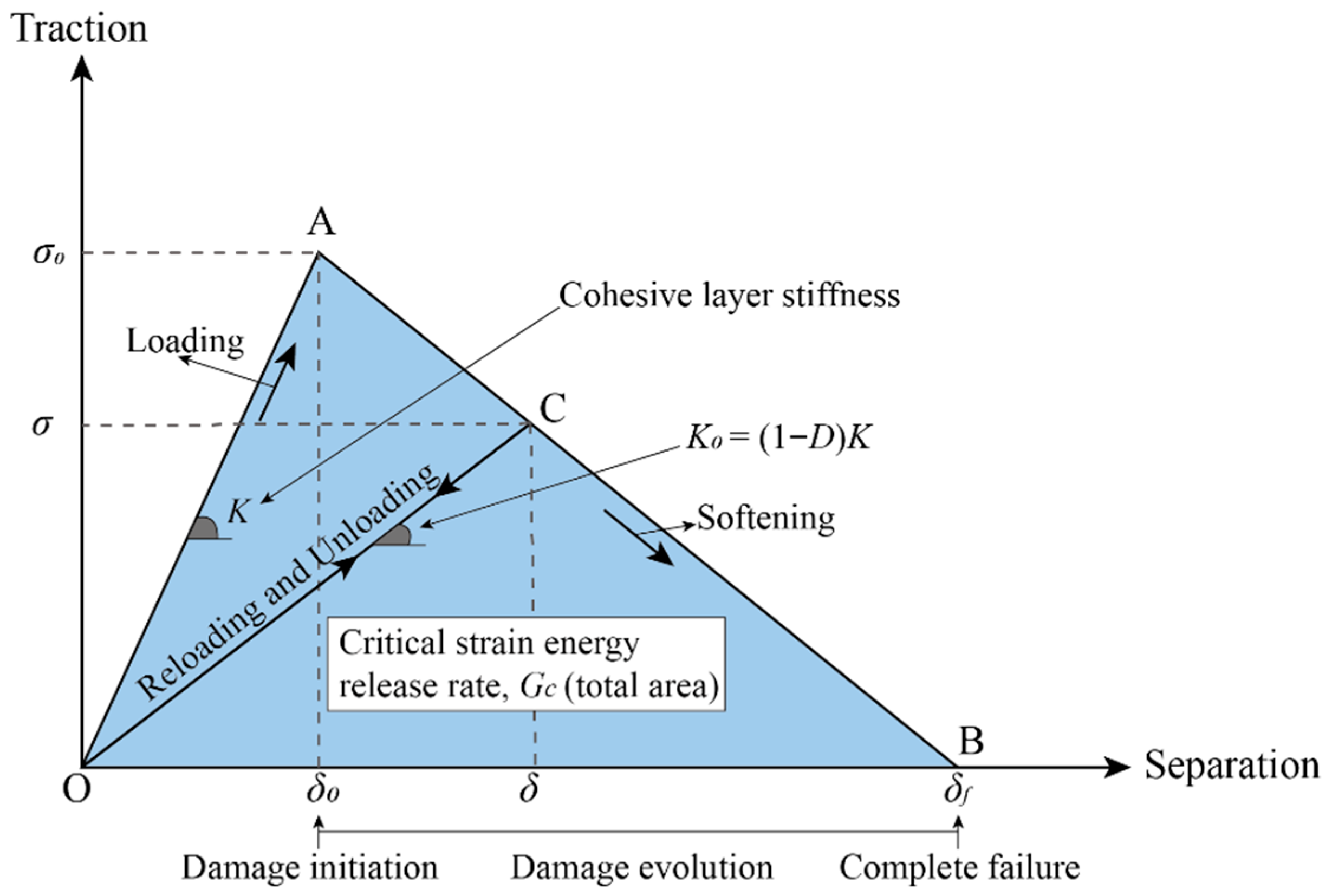
As shown in Figure 3, a typical bilinear traction–separation law (TSL) model is used to describe the slope characteristics of interface behavior. The initial stage is a linear elastic loading stage, and the material exhibits linear elastic behavior before reaching its strength limit. Then it enters the softening stage (AB), when the stiffness decreases linearly after the material reaches its strength limit. In the unloading stage (CO) and the subsequent reloading stage (OC), the material exhibits linear elastic behavior along the line OC and shows a gentle slope ($K_0$) in order to describe the behavior after the peak, a bilinear softening evolution function containing the damage variable D is used, where the value of D ranges from 0 to 1.

$$K_0=(1-D)K,$$

(11)

$${\displaystyle \frac{\sigma }{\delta }}=(1-D){\displaystyle \frac{{\sigma }_0}{{\delta }_0}},$$

(12)

$$D=1-{\displaystyle \frac{{\delta }_0\sigma }{\delta {\sigma }_0}}=1-{\displaystyle \frac{{\delta }_0}{\delta }}{\displaystyle \frac{({\delta }_f-\delta )}{({\delta }_f-{\delta }_0)}}={\displaystyle \frac{{\delta }_f(\delta -{\delta }_0)}{\delta ({\delta }_f-{\delta }_0)}},$$

(13)

Figure 3. A typical bilinear TSL for cohesive element.

Among them, $K$ is the cohesive stiffness; $K_0$ is the stiffness during unloading or reloading; ${\sigma }_0$ and ${\delta }_0$ are the critical stress and critical displacement at the onset of damage; $\sigma$ and $\delta$ are the critical stress and critical displacement in the softening stage; and ${\delta }_f$ is the critical displacement at complete separation.

As the material separation increases, the traction force gradually increases until it reaches a peak value at point A, which corresponds to the point on the separation axis called the damage initiation point ${\delta }_0$. Debonding and damage initiation occur at point A, and the subsequent process is called the linear softening or damage evolution stage, which ends at point B. At point B, the traction force value drops to zero, corresponding to the maximum separation and damage value of 1.

2.2.2. Generation of Cohesive Elements

There are two main methods for CZM: cohesive elements and cohesive surfaces. In this study, a cohesive zone model designed specifically for cohesive elements is used. As shown in Figure 4, the cohesive zone has basic geometric properties, including geometric thickness and constitutive thickness. The geometric thickness represents the physical size of the model, while the constitutive thickness is the size used for internal calculations in the model. In order to achieve a cohesive zone with discretized thickness, a layer of cohesive elements is required in the model. It should be noted that at least one of the two surfaces (upper or lower surface) of the cohesive zone must be connected to other components. It is best practice to connect both surfaces of the cohesive zone to adjacent components to avoid abnormal deformation patterns that may be caused by single-surface connection. In this study, the cohesive zone is matched with the adjacent landslide mesh and directly connected through shared nodes, as shown in Figure 4a. Figure 4b shows a schematic diagram of the cohesive zone in the two-dimensional model.

Figure 4. The structure of cohesive elements.

However, to accurately simulate the behavior of a specific material, the CZM requires suitable parameters, such as fracture energy and interface strength. The determination of these parameters usually requires extensive experiments or the application of inverse problem solving techniques. In addition, in order to accurately simulate crack growth and material fracture, the CZM usually requires the use of a fine finite element mesh near the crack front or interface. This means that additional finite elements are needed to fully represent the interface.

2.3. LEM and CZM Coupled Simulation Process

This paper proposes a landslide simulation method based on the combination of LEM and CZM. By integrating sliding surface identification, crack evolution modeling, and landslide dynamic response analysis, the physical reconstruction of the whole process of landslide damage from potential instability to final sliding is realized. First, the slope geometry information is modeled on the Rhino platform and divided into multiple closed polyline regions according to the strata. The self-written script exports its node coordinates into a standard text format and uniformly processes them in Python. The program calls the Pyclipper library to perform Boolean operations on the boundaries of different strata to construct the outer contour of the complete slope. Pyclipper uses integer coordinates rather than floating-point numbers for geometric calculations. This design may introduce rounding errors and geometric tolerance issues, which could result in errors due to integer precision. Considering that Pyclipper uses integer precision, in order to avoid numerical errors, the coordinates are uniformly scaled and retained to three decimal places before processing. Subsequently, dense grid nodes are generated in the slope area as potential sliding circle centers, and the arc radius range is defined in combination with the surface boundary to automatically generate a large number of candidate sliding surfaces. The candidate surfaces are circular arcs generated through the following rigorous geometric constraints: center distribution, radius control, and intersection criterion. The program performs geometric screening on each arc and only retains valid sliding surfaces with two intersections with the slope contour to ensure physical rationality and improve computational efficiency. For each effective sliding surface, the program automatically divides the sliding area into multiple soil strips, extracts its geometric parameters, and uses the simplified Bishop method to perform stability analysis. The corresponding safety factor is obtained through iterative calculation, and finally the dangerous sliding surface with the minimum safety factor is selected.

After obtaining the sliding surface, the program further partitions the overall slope spatially, dividing the slope into two parts: a potential sliding body and a stable foundation. The sliding surface serves as the interface of the subsequent crack propagation path. To simulate the interface rupture process, this paper introduces CZM units on the shared unit surface inside the sliding body, and automatically inserts thickness-free cohesive units to characterize the interface damage evolution behavior. The generation of cohesive units is completed by a self-written script. The script first identifies various units and their topological connection relationships in the INP file, extracts all unit surface information, and counts the frequency of shared surfaces, from which internal interfaces shared only by two units are selected; for these interfaces, adjacent units have their own independent node surfaces by copying and renumbering nodes, and then cohesive units such as COH2D4 are inserted between the two node surfaces, and corresponding Elset information is created to ensure that the model structure is continuous and topologically correct. After the generated cohesive units are imported through ABAQUS, material parameters based on the bilinear TSL can be assigned, including normal/tangential limit stress, fracture energy, and critical separation displacement. The CZM unit can thus simulate the interface strain softening and final complete separation and thus reproduce the initiation and propagation of cracks on the sliding surface and the complete sliding process of the sliding body.

2.3.1. LEM-to-CZM Data Transfer, Assumptions, and Boundary Conditions

To guarantee a mechanically consistent transition from the LEM stability calculation to the CZM fracture simulation, a one-way, non-iterative mapping protocol is executed immediately after the critical slip surface $𝒫$LEM is identified. The detailed steps are as follows:

(1)

Stress recovery from LEM

For each slice base segment i, the effective normal stress and mobilized shear stress are recovered from the final Bishop iteration:

These scalar values are linearly interpolated onto the vertices of $𝒫$LEM to produce two continuous traction profiles.

(2)

Key mapping assumptions

The slip surface is assumed to be a zero-thickness internal boundary governed exclusively by mixed-mode (I + II) cohesive separation; out-of-plane shearing (mode III) is neglected because the 2-D LEM provides no information on that component.

The interpolated tractions are imposed as initial cohesive tractions at zero separation (δ_n = δ_s = 0) by means of the ABAQUS keyword *INITIAL CONDITIONS, TYPE = TRACTION. This pre-stresses the CZM elements to the limit-equilibrium state and eliminates the need for an additional gravity ramp-up step.

Pore-water pressures u(s) extracted from the LEM iteration are kept frozen throughout the CZM analysis; hydro-mechanical coupling is intentionally deactivated to honor the one-way coupling strategy.

(3)

Mesh partitioning and node duplication

A Python script automatically duplicates all nodes located on LEM and assigns unique IDs. Zero-thickness cohesive elements (COH2D4 for 2-D) are inserted between the duplicated node pairs. Each cohesive element inherits the interpolated tractions at its centroid and stores them as the .Inp deck.

(4)

Boundary and loading conditions for the CZM stage

Far-field boundaries remain identical to the LEM model: roller constraints on lateral sides and full fixity at the base.

Because initial tractions are already in global equilibrium with gravity, no additional gravity step is executed; the explicit simulation starts with a quasi-static “release” step (time = 0) followed by a dynamic step with mass-proportional damping (α = 0.05).

The ground surface is kept traction-free, while the lower block (stable substratum) is constrained against rigid-body motion. The upper block (sliding mass) is free to displace once the cohesive tractions drop to zero, thus reproducing the transition from progressive failure to catastrophic sliding.

(5)

Verification and tolerance checks

Prior to the dynamic step, a zero-displacement equilibrium check is performed: with all cohesive elements artificially rigid, the maximum nodal unbalanced force must be <0.1% of the characteristic gravitational force. If this tolerance is violated, the LEM slice discretisation is locally refined and the mapping is repeated.

After completing the model construction and parameter assignment, the ABAQUS explicit dynamics module was used for numerical simulation, setting appropriate gravity fields, boundary conditions, and mass damping to capture key responses such as the rupture path of the landslide, the evolution of cracks, and the sliding velocity in real time. This simulation process effectively realizes the coupled modeling of the entire process from sliding surface identification to crack development to overall sliding, providing a reliable numerical tool and physical basis for understanding the rupture mechanism and energy dissipation path of the landslide.

2.3.2. Mesh Discretisation and Sensitivity Analysis

All continuum domains were discretised using 8-node linear hexahedral elements (C2D4) with an average global seed size of 0.5 m, yielding approximately 12,000 elements for the EX11 slope model.

In the monitoring process, the mesh sensitivity was studied by global refinement of the seed size from 1.0 m → 0.5 m → 0.25 m. The safety factor (F_s), the maximum displacement after failure (U_max), and the calculation cost (CPU time ∝ number of elements) under different mesh sizes were analyzed, as shown in Table 1.

Table 1. Analysis results of different mesh sizes.

Grid Size	Fs	Umax (m)	Tcpu (h)
1 m	1.42	4.12	0.3
0.5 m	1.39	3.65	1.1
0.25 m	1.38	2.18	4.8

Results indicated that 0.5 m achieved an optimal balance between accuracy and efficiency, and was therefore adopted for all subsequent simulations.

2.3.3. Cohesive Zone Parameters: Calibration and Justification

This paper calibrated the bilinear TSL by referencing prior literature [29,30]. Sensitivity to Gf was further explored by varying ±25%; resultant run-out changed <5%, confirming robustness.

3. Results

3.1. Analysis of the Results of EX11

To validate the slope stability coefficient calculation, the author’s program results are compared with established international case studies, confirming their accuracy. The Australian Computer Applications Association surveyed slope stability analysis software usage in Australia through a five-question exam study. The survey designed five examination questions, and Prof. Fredlund of Saskatchewan University in Canada and Prof. Baker of Israel Institute of Technology provided reference answers. In this paper, the stability coefficient of EX11 is calculated, which is homogeneous slope material parameters, as shown in Table 2 [31].

Table 2. Assessment Question EX11 Material Properties.

Assessment Question	c(kN/m2)	γ(kN/m3)
EX11	3.0	20.0

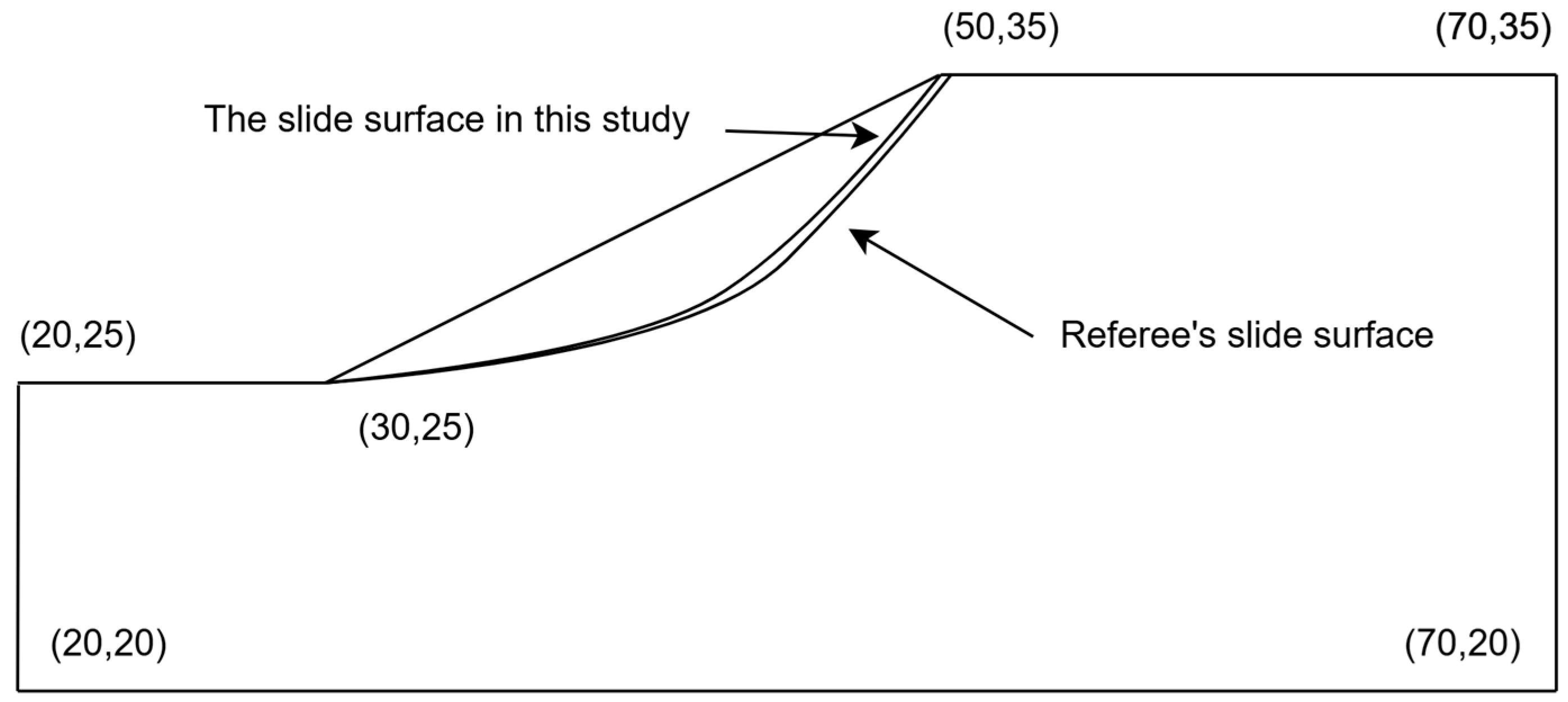
For exam question EX11, the minimum Factor of safety calculated in this work was 0.986, which is close to the referee’s recommendation as shown in Figure 5. The result proves the reliability of determining the slip surface by the stability coefficient in this paper.

Figure 5. Example of the sliding surface of the slope in EX11.

The specific simulation flow chart of this paper is shown in Figure 6, which mainly realizes the generation of cohesive elements by writing a script. The script can automatically insert cohesive elements between the shared surfaces of the specified unit set to simulate material interface debonding or crack propagation. The implementation method is as follows.

Figure 6. LEM–CZM modeling process for EX11 example.

Within the ABAQUS/Explicit environment (Dassault Systèmes, 2023), the mesh information including node, element, and elset, is obtained through reading INP files with regular expressions. According to elset information, the meshes are divided into the slide body and other sets. Each node on the mesh is assigned to a new node id, and each element is separated into an independent grid without connected nodes. In this way, the face of each element is generated with new node ids. Looping for all faces of elements and counting the number of occurrences of shared faces, the internal faces and external faces are identified. Internal shared faces are inserted into zero-thickness 4-node quadrilateral interface (COH2D4) elements—each possessing three translational degrees of freedom per node, one integration point, and support for finite-sliding, large-strain, and mixed-mode traction–separation laws, while external faces that coincide with model boundaries are ignored to avoid spurious debonding. The node connection relationship of the cohesive elements is determined by mapping the old and new nodes. The element connection relationship is updated to ensure the mesh continuity of the non-sticky area.

With the new node, element, and elset, a new INP file can be generated. To guarantee ID uniqueness, the sticky unit ID starts at max(solid ID) + 1 and is incremented sequentially without gaps. By copying nodes, detecting shared faces, and stitching non-interface nodes, batch adding COH units in complex grids can be achieved, significantly improving the efficiency of establishing interface models.

In the subsequent CZM analysis, the slope is divided into the landslide area and the foundation area according to the most dangerous sliding surface. The CZM is inserted into the landslide area to simulate the crack development of the sliding surface. The slope sliding surface simulated by the ACADS slope stability analysis test question EX1 is restored one-to-one. The material parameters are shown in Table 3.

Table 3. Initial Model—Assessment Question EX11 Material Properties.

Assessment Question	c (kN/m2)	γ (kN/m3)	φ/°
EX11	3.0	20.0	19.6

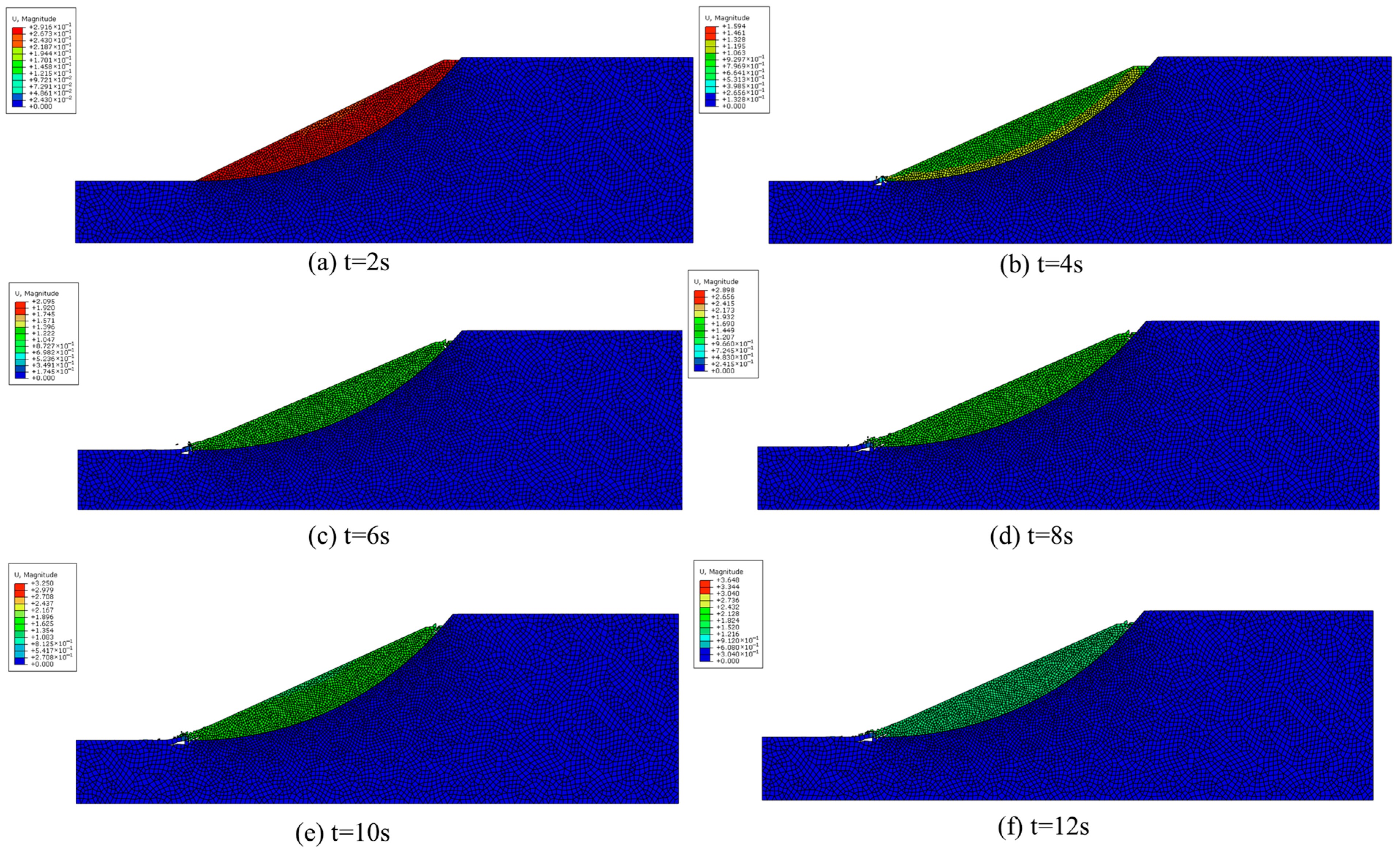
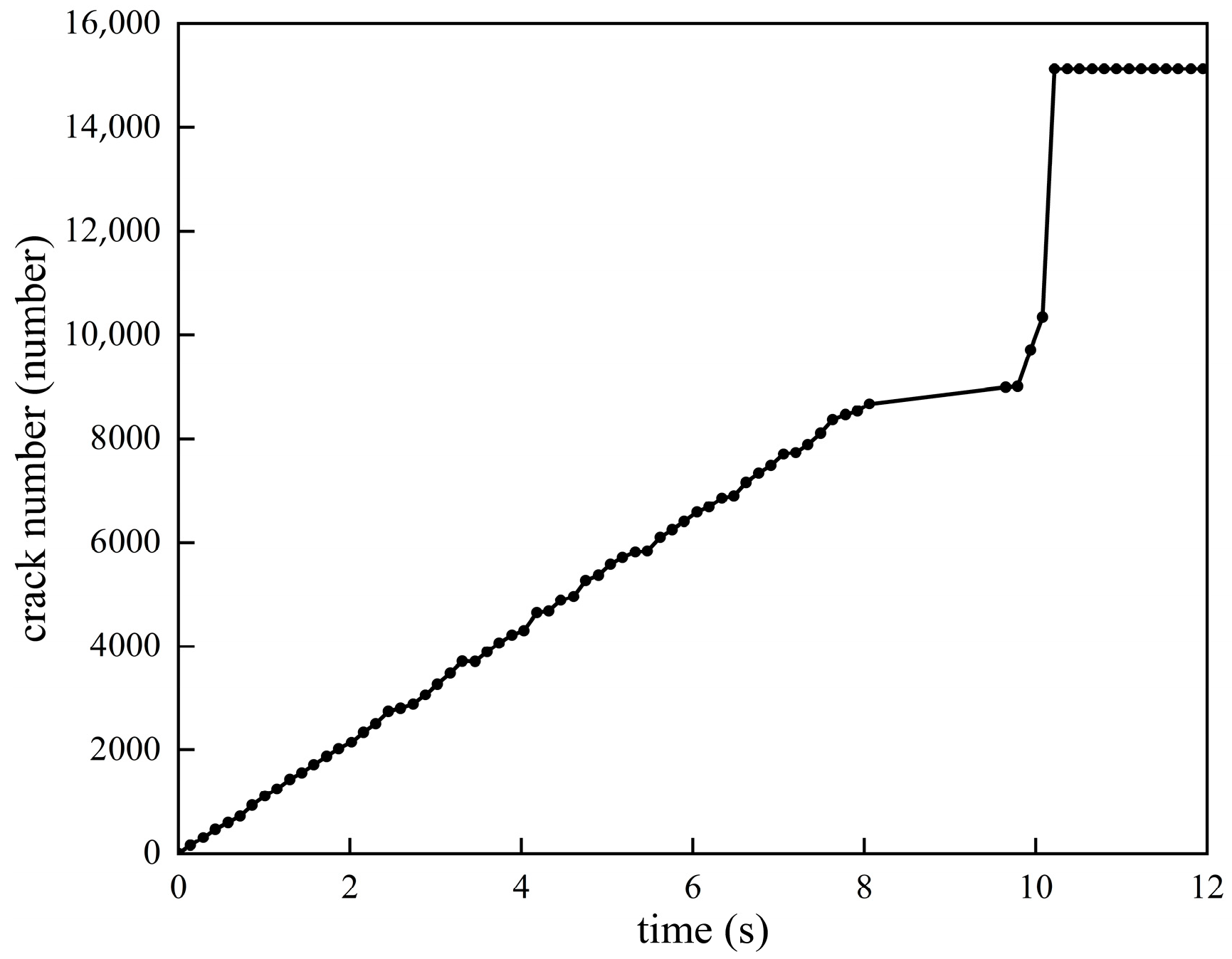
In order to understand the crack development process of the sliding surface, Figure 7 and Figure 8 show the displacement cloud diagram and the number of cracks generated by the landslide movement at different times and analyze its movement law:

Figure 7. Loud map of crack development displacement on the sliding surface.

Figure 8. The number of cracks changes at different times.

According to the displacement nephograms at six times (2 s, 4 s, 6 s, 8 s, 10 s, and 12 s) and the maximum displacement in the legend, the sliding process on the sliding surface can be divided into three stages, as shown in Table 4.

Table 4. Deformation characteristics of landslide sliding surface.

Deformation Stage	Time (s)	Maximum Displacement U_max (m)	Crack Number (Number)	Crack Growth Rates (Number/s)
Crack initiation and sliding initiation stage	T = 2	2.92 × 10−1	2149	1074.5
The stage of crack propagation and foundation separation	T = 4	1.59	4299	1075
	T = 6	2.10	6589	1145
The sliding stage of the ruptured landslide	T = 8	2.90	8671	1041
	T = 10	3.25	10,341	835
	T = 12	3.65	15,131	2395

(1) Crack initiation and sliding initiation stage (t = 2 s)

Maximum displacement $U_{max}$ ≈ 2.92 × 10⁻¹ m (see the red scale in Figure 7a). The rupture first initiated at the top of the sliding surface (the contact between the landslide and the foundation), and the top unit changed from red to yellow to green, indicating that the strain was concentrated and slipped first. No obvious displacement has occurred at the bottom, indicating that the initial cracks are confined to the top of the sliding surface.

(2) The stage of crack propagation and foundation separation (t = 4–6 s),

$U_{max}$ ≈ 1.59 m at t = 4 s and $U_{max}$ ≈ 2.10 m at t = 6 s (see Figure 7b,c). The cracks spread upward rapidly along the established sliding surface, and the central unit changes from orange to red. The red high displacement zone also begins to appear at the bottom, indicating that the middle and lower parts of the landslide have basically separated from the lower part. The large area CZM element on the failure surface breaks and fails, and the interior of the sliding mass enters “Block” state, and the maximum displacement gradient zone gradually moves from the middle to the bottom.

(3) The sliding stage of the ruptured landslide (t = 8–12 s),

$U_{max}$ ≈ 2.90 m at t = 8 s, $U_{max}$ ≈ 3.25 m at t = 10 s, and $U_{max}$ ≈ 3.65 m at t = 12 s (see Figure 7d–f). The entire sliding body area is almost all red, indicating that the cohesion is depleted and the sliding body is sliding as a rigid body. The distribution of the displacement field tends to be uniform, and the $U_{max}$ increases linearly with time. The average slip velocity is about 1.7 m/s; this speed is as expected.

3.2. Analysis of the Results of Real Slope

3.2.1. Geological Background

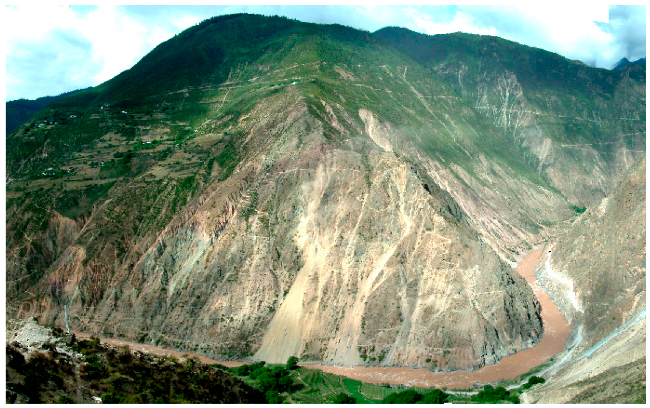
In order to verify the correctness of the calculation of the slope stability coefficient, an engineering slope will be used for analysis. The engineering slope is shown in Figure 9.

Figure 9. The real landslide shape diagram of the project.

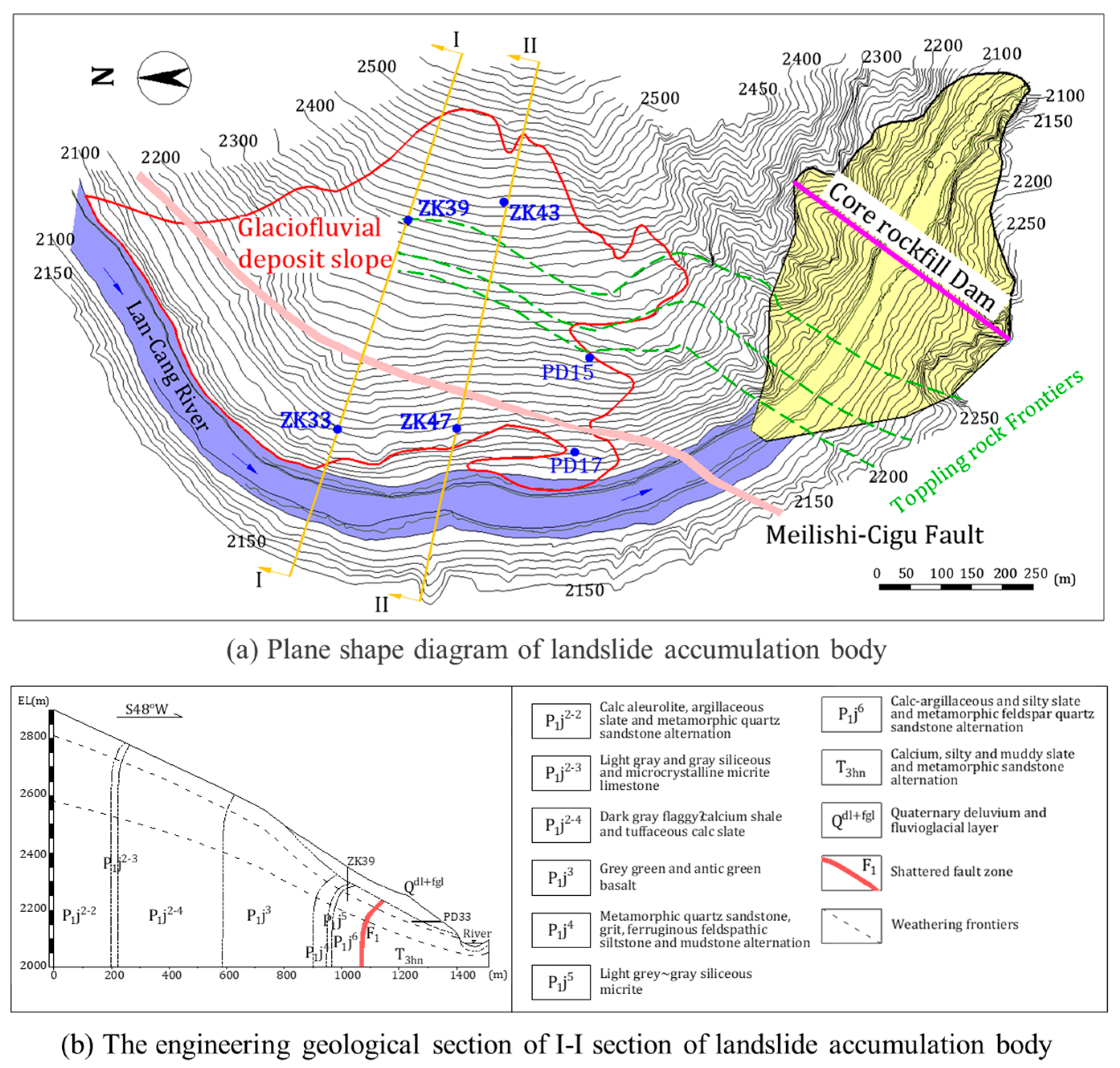
The landslide is located near the Lancang River in Yunnan Province. The specific plane shape map and engineering geological map are shown in Figure 10. The terrain on both sides of the landslide area is steep. The lithology of the exposed strata on both sides is mainly Jurassic, Triassic clastic rocks, and Permian mild metamorphic rocks. The development of the river valley is obviously controlled by the structure, and the reservoir bank slopes are mostly along oblique valleys. The three major rocks of sedimentary rock, magmatic rock, and metamorphic rock, in the area are exposed. Among them, the Lower Paleozoic Silurian and Ordovician are missing, the Mesozoic Cretaceous and Jurassic are partially missing, and the Upper Paleozoic strata are the most widely distributed. In addition to the Cenozoic strata, the strata of the other ages are subjected to different degrees of metamorphism. The area is dry and has less rain; the average annual precipitation is 494.7~522.4 mm, and the vegetation on both sides of the reservoir area is scarce. The hydrogeological conditions of the reservoir area are relatively simple: the spring point is exposed higher, the groundwater level on both sides of the Lancang River is higher than the river water, and the Lancang River is the lowest discharge datum in the area.

Figure 10. Landslide plane diagram and engineering geological map (according to the literature [32] change).

The recharge sources of groundwater are mainly snow melting water and atmospheric precipitation, mainly snow water recharge, followed by atmospheric precipitation.

(1) Melting water of ice and snow: In the reservoir area, the annual snow cover is 5~6 months at the elevation of 3000~3500 m, the annual snow cover is 6~7 months at the elevation of 4000~5000 m, the annual snow cover is more than 5000 m, and the winter snow line drops to about 2500 m. The melting of ice and snow is the most important water source in the area, and the water storage is quite abundant.

(2) Atmospheric precipitation: The Lancang River belongs to the alpine gorge zone, which is located in the subtropical marginal climate zone. Due to the influence of elevation and topography, the atmospheric precipitation changes greatly, and changes obviously with elevation. In the valley zone, the annual rainfall is less, the surface vegetation is less or no vegetation, and the precipitation is small. With the increase in terrain, the temperature gradually decreases, and the rainfall is concentrated in the alpine zone.

3.2.2. LEM Modeling for Safety Factor

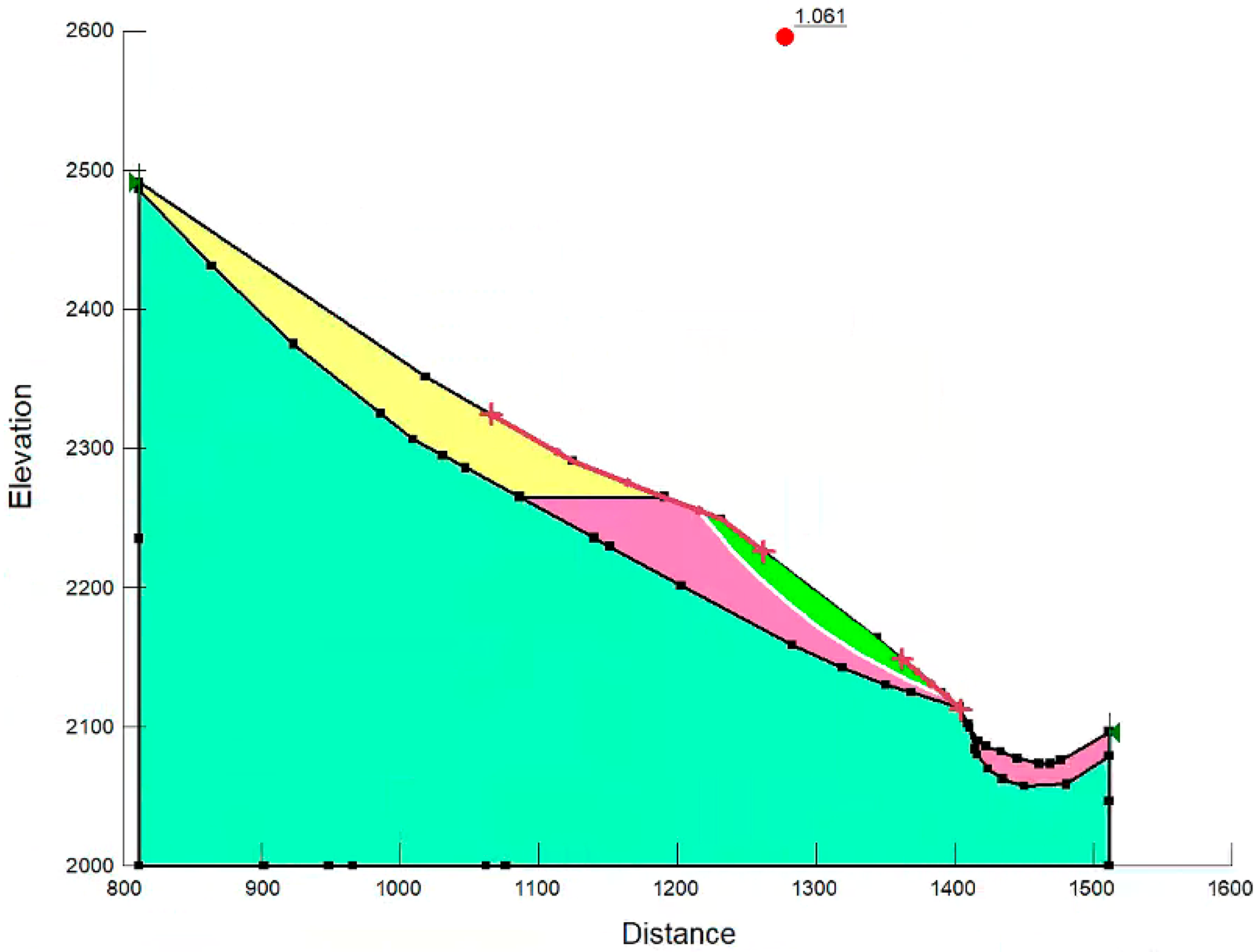
Using Geostudio 2023 software, the geometric model of landslide profile is established in SLOPE/W module. The specific material parameters are shown in Table 5. The circular sliding surface is determined by LEM, and the safety factor is calculated to be 1.061, as shown in Figure 11.

Table 5. Material properties of slope.

Components	Unit Weight (kN/m3)	Cohesion (kPa)	Friction Angle (°)
Foundation area	25	4500	48.0
Accumulation body	21	25	28.5

Figure 11. Calculation results of landslide safety factor with 1.061.

3.2.3. CZM Modeling for Landslide Hazard

The LEM-based landslide model was originally established in GeoStudio (SLOPE/W module) to determine the critical slip surface and the corresponding safety factor. Subsequently, the geometric sections containing material partition and slip surface information are exported in DXF format and imported into Rhino to generate high-quality structured grids, so as to ensure the numerical stability and accuracy of subsequent finite element simulation. Through the self-compiled Python script, the grid data is converted into Abaqus-readable INP input file, and the node coordinates, unit connections, and material properties are completely retained.

In Abaqus, another Python script is used to insert the cohesive element (COH2D4) along the preset slip surface in batches to simulate the progressive failure and post-peak softening behavior of the landslide. The cohesive constitutive uses the traction–separation law to define the peak and residual strength, fracture energy, and damage evolution considering the failure mode, so as to truly reflect the strength degradation of the interface under shear or tension-shear combined action.

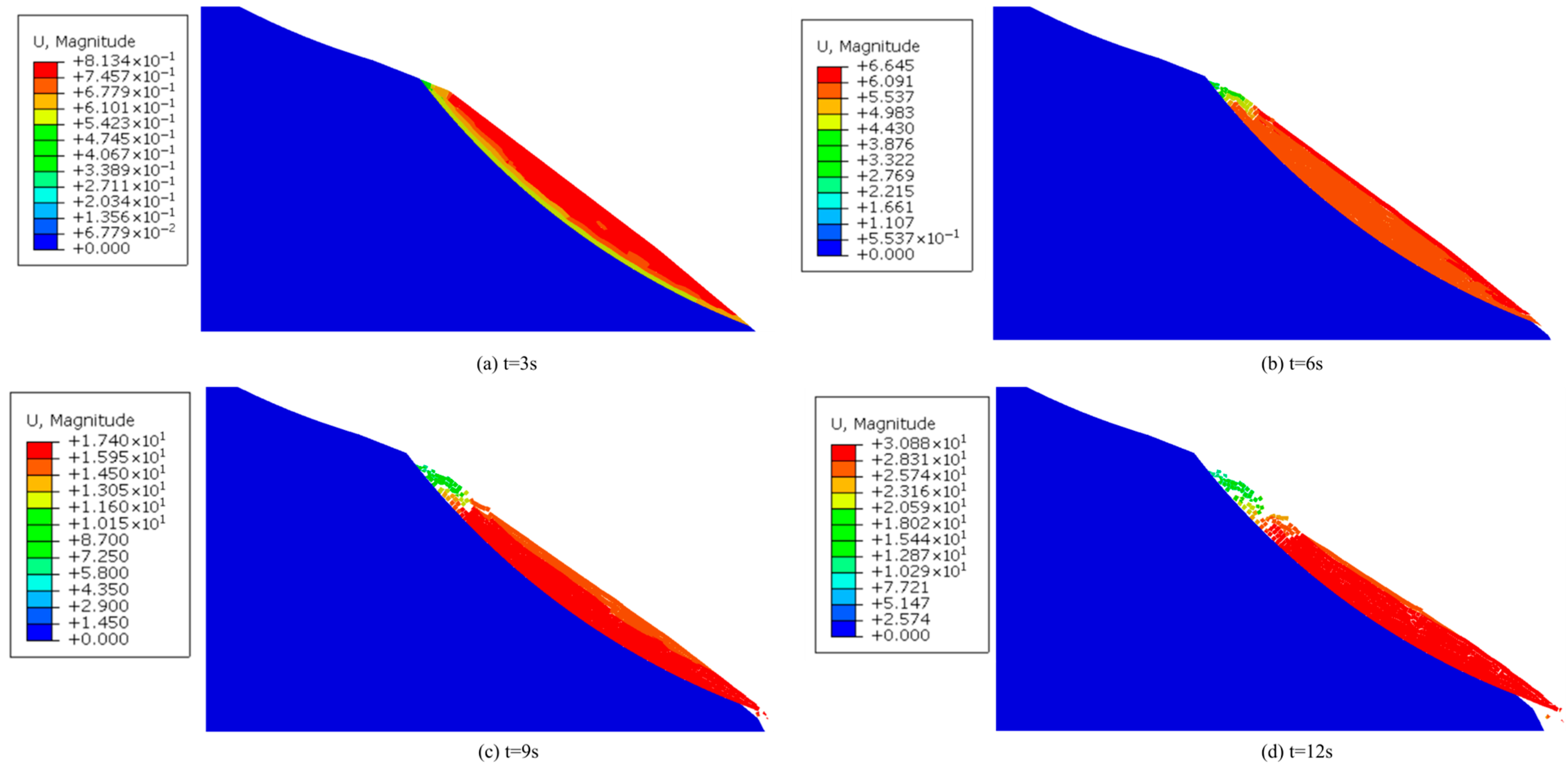
Through dynamic explicit analysis, the development process of slope instability with time is tracked. Figure 12 shows the displacement contours at different times: U_max ≈ 0.81 m at t = 3 s, U_max ≈ 6.65 m at t = 6 s, U_max ≈ 17.40 m at t = 9 s, and U_max ≈ 30.88 m at t = 12 s. The accelerated growth of displacement indicates that the landslide gradually evolves from initial initiation to large-scale sliding, which is consistent with the characteristics of landslide movement observed in the field. The coupled LEM–CZM numerical framework proposed in this paper provides a robust framework for predicting landslide initiation and movement path, and can provide an important basis for disaster assessment and prevention design.

Figure 12. Displacement cloud map of engineering landslide at different times.

4. Discussion

An LEM–CZM framework for simulating slope failure is proposed. The above content has shown the ability of the framework. Here, the feasibility of the framework is discussed by giving different parameters. In this section, two influencing factors of fracture parameters and friction parameters are discussed.

4.1. Effect of Fracture Parameters

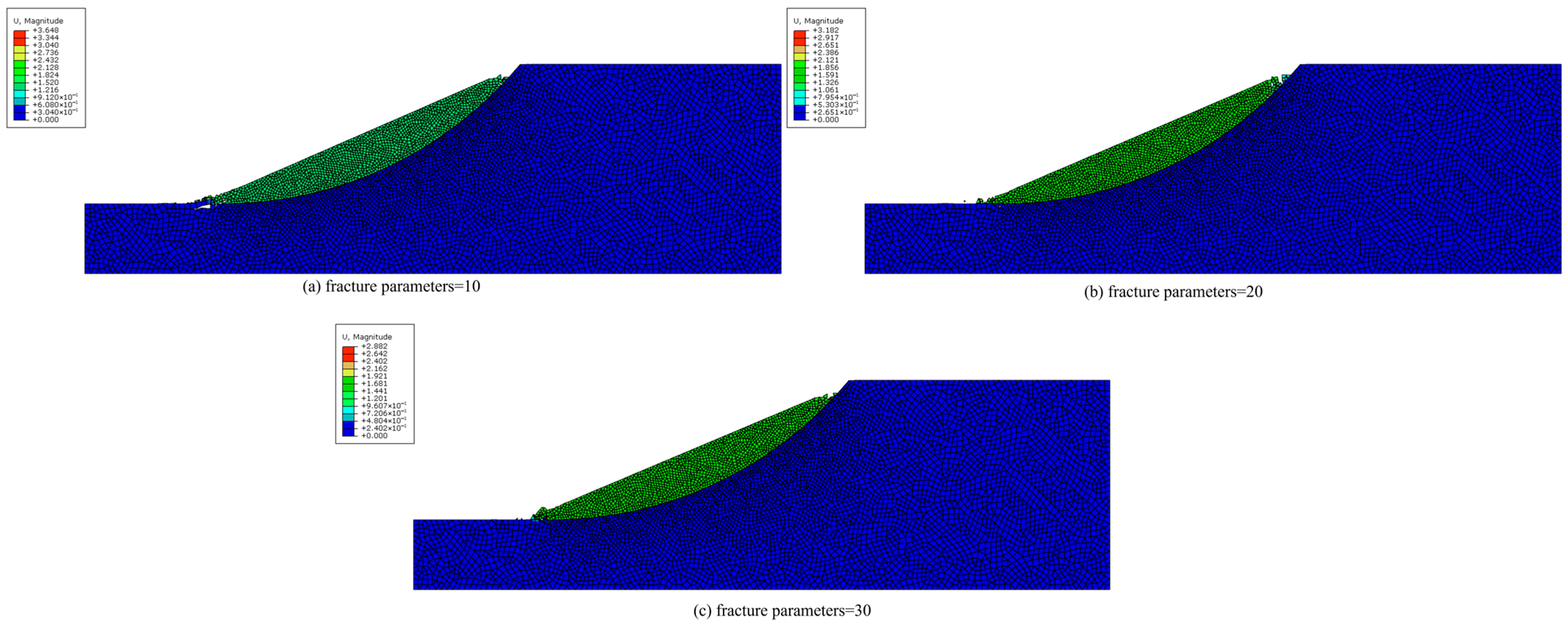
The landslide displacement cloud diagram under different fracture parameters was calculated by numerical simulation. The fracture parameters are 10, 20, and 30, respectively, and the landslide displacement cloud map is shown in Figure 13. The displacement contour maps in Figure 13 correspond to interface fracture energy values G_f = 10, 20, and 30 J/m², respectively. The observed reduction in maximum landslide displacement ($U_{max}$) from 3.65 m to 2.88 m is governed by the energy-based crack propagation criterion of the cohesive zone model:

$$\mathrm{G}={\displaystyle \frac{{\mathrm{K}}_{\mathrm{I}}^2}{{\mathrm{E}}^{\prime }}}\ge {\mathrm{G}}_{\mathrm{f}}$$

(14)

where G is the energy release rate and the unit is N/m; ${\mathrm{K}}_{\mathrm{I}}$ is the type I stress intensity factor and the unit is Pa·m^1/2; $E^{\prime }$ is the effective elastic modulus; ${\mathrm{G}}_{\mathrm{f}}$ is the fracture toughness and the unit is N/m.

Figure 13. Displacement cloud diagram under different fracture parameters.

As $G_f$ increases, a higher mode ${\mathrm{K}}_{\mathrm{I}}$ is required at the crack tip to trigger interface softening. This delays crack propagation, increases energy dissipation along the slip surface, and reduces the final runout distance. Mechanistically, this implies that engineering measures such as grouting or geosynthetic reinforcement, which enhance ${\mathrm{G}}_{\mathrm{f}}$ by ≥50%, can effectively reduce post-failure displacement by approximately 20% under the current slope geometry and stress conditions. With the increase in fracture parameters, the maximum displacement $U_{max}$ of the landslide decreases gradually, indicating that the bearing capacity of the landslide increases gradually. The specific performance is that when the fracture parameters increase from 10 to 20, $U_{max}$ decreases from 3.65 m to 3.18 m. When the fracture parameters increase from 20 to 30, $U_{max}$ decreases from 3.18 m to 2.88 m. The essence of this law is that the fracture parameters directly determine the ability of rock and soil to resist crack initiation and propagation, and the degree of crack development is directly related to the structural integrity and anti-sliding stability of the landslide. This law also provides key guidance for landslide prevention and control engineering: improving the fracture parameters of rock and soil mass through grouting reinforcement, bolt support, and other measures can effectively reduce the maximum displacement of the landslide and enhance its bearing capacity, so as to ensure the stability of the slope.

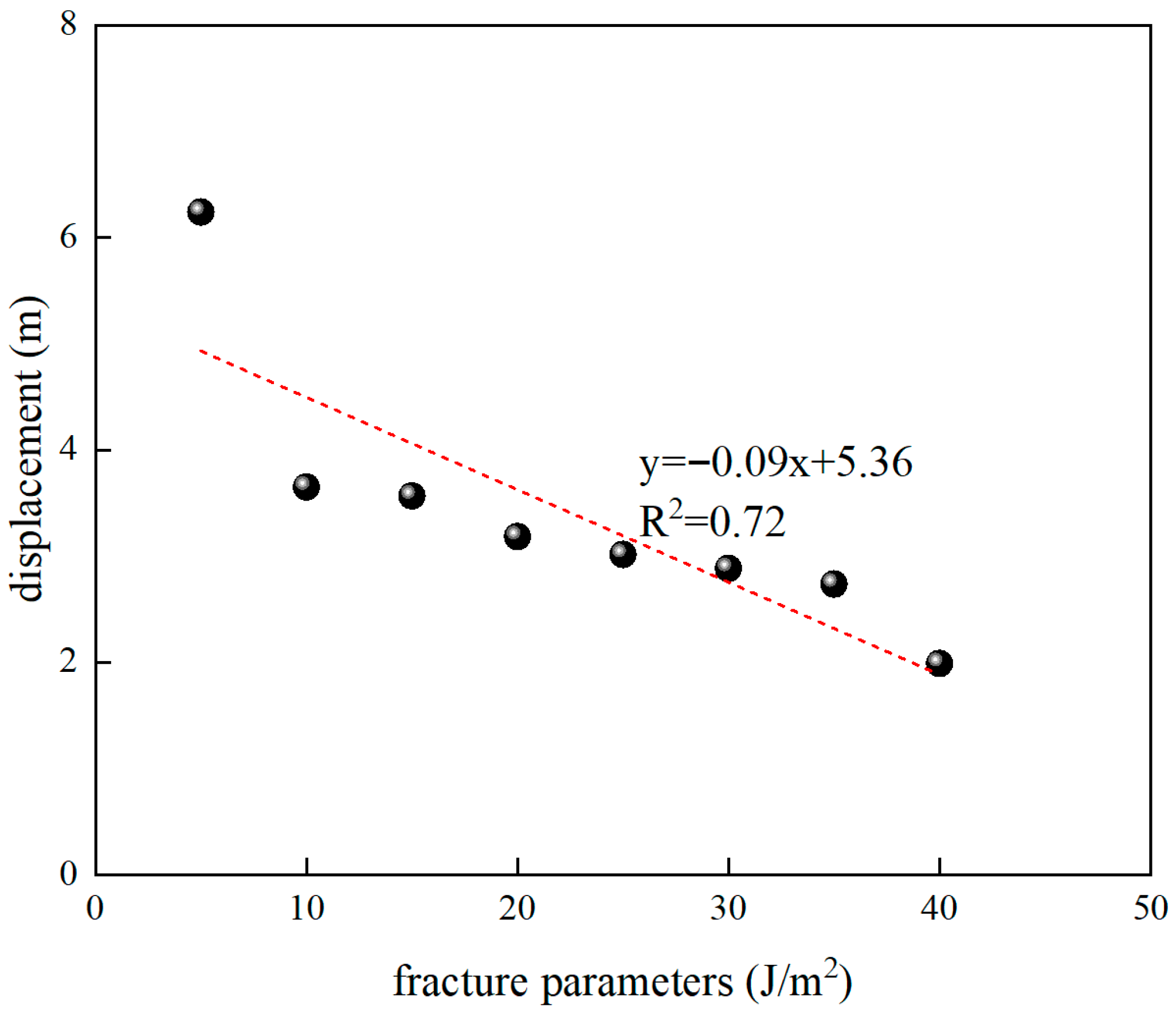
Figure 14 shows the relationship between displacement and fracture parameters, and linear regression fitting shows that the fitting equation is y = −0.09x + 5.36, and the fitting degree R² = 0.72. It shows that the displacement is negatively correlated with the fracture parameters, and the displacement decreases with the increase in the fracture parameters.

Figure 14. The relationship curve between displacement and fracture energy.

4.2. Effect of Friction Parameters

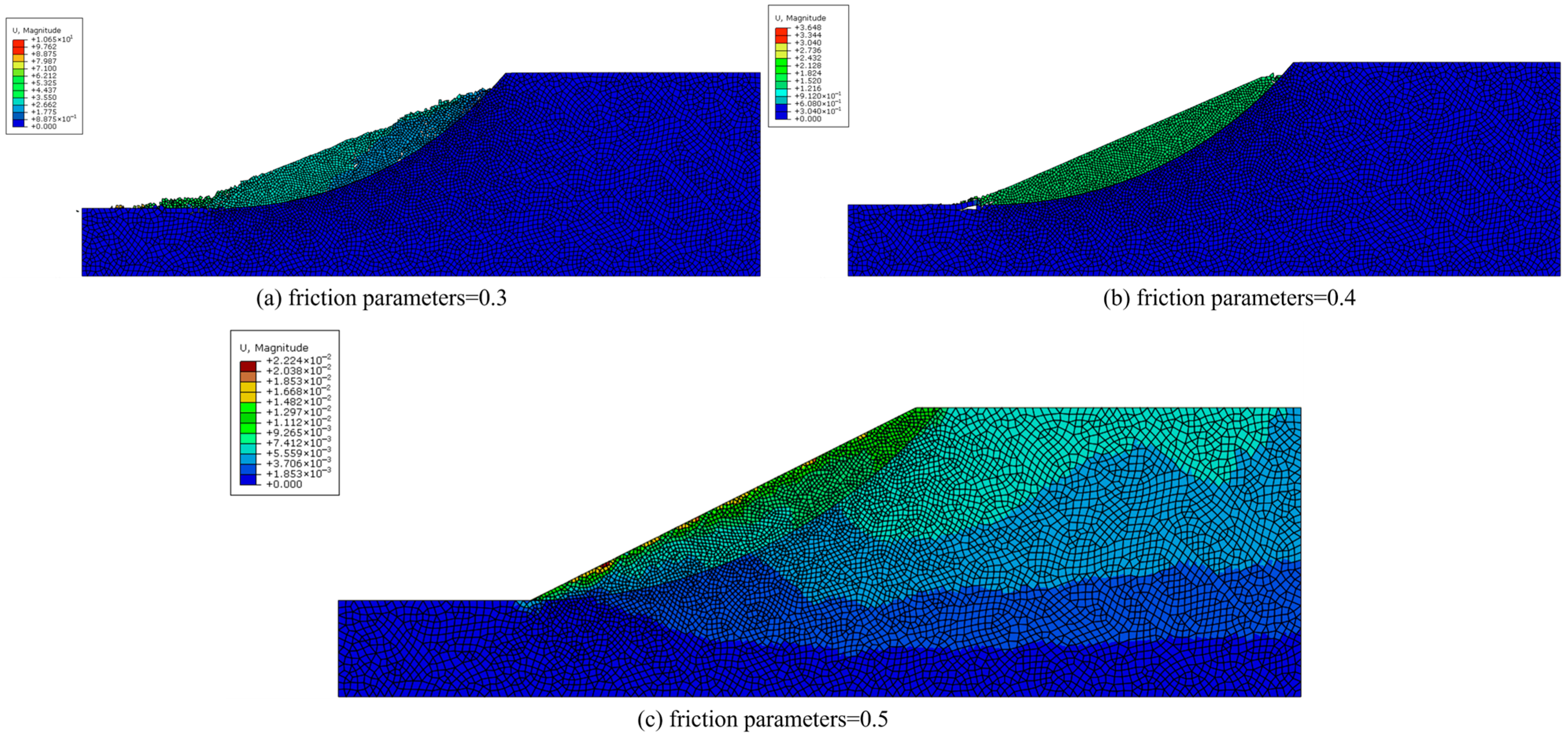
The landslide displacement cloud diagram under different friction parameters is calculated by numerical simulation. The fracture parameters are 0.3, 0.4, and 0.5, respectively, and the landslide displacement cloud map is shown in Figure 15. Figure 15a–c present displacement fields for interface friction coefficients μ = 0.3, 0.4, and 0.5 (see caption). The underlying mechanism lies in the shear traction–separation law of the mixed-mode cohesive zone model:

$$\mathsf{\tau }=\mathsf{\mu }{\mathsf{\sigma }}_{\mathrm{n}}\left(1-\mathrm{D}\right)$$

(15)

where $\mathsf{\mu }$ is the effective friction coefficient. Increasing μ directly raises the elastic shear strength envelope, delaying the onset of damage (D > 0) and shifting the softening branch to larger slip displacements. At μ = 0.5, the energy release rate along the interface remains below the fracture energy, preventing full damage development (D < 1) and arresting the slope in a metastable state. This mechanistic insight explains why enhancing basal roughness—through measures such as bench-terracing or rock-bolt shear keys—can convert an unstable landslide into controlled creep, thereby improving slope stability. Its influence mechanism can be intuitively reflected by the displacement response and mechanical equilibrium state in the process of landslide instability. From the quantitative results, with the gradual increase in friction parameters (taking friction coefficient as an example), the $U_{max}$ of the landslide body shows a monotonically decreasing trend. When the friction coefficient increases from 0.3 to 0.4, $U_{max}$ drops from 10.65 m down to 3.68 m. When the friction coefficient increases to the critical threshold of 0.5, the landslide body is completely in a mechanical equilibrium state, and there is no obvious sliding trend in the simulated loading period. This phenomenon confirms the positive correlation between the friction parameters and the bearing capacity of the landslide. The research results provide important theoretical support for landslide engineering treatment. The actual project can improve the friction parameters in a targeted manner and then realize the long-term improvement of slope stability by reducing the maximum displacement of the landslide and enhancing the bearing capacity.

Figure 15. Displacement cloud diagram under different friction parameters.

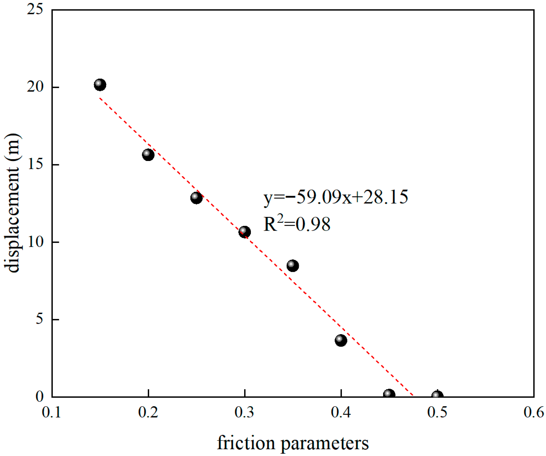
Figure 16 shows the relationship between displacement and friction parameters, and linear regression fitting shows that the fitting equation is y = −59.09x + 28.15, and the fitting degree R² = 0.98. It shows that the displacement is negatively correlated with the friction parameters, and the displacement decreases with the increase in the friction parameters.

Figure 16. The relationship curve between displacement and friction parameters.

4.3. Comparison with Traditional LEM and FEM

In this paper, the LEM–CZM method is reanalyzed in Abaqus 2023. Comparing traditional LEM and SRM-FEM, Table 6 summarizes the comparison results. The three models use the same material parameters, boundary conditions, and hardware platform. The accuracy of LEM–CZM is the same as that of Bishop LEM in reproducing the classical safety factor, and the difference between the post-sliding displacement and the high-resolution SRM-FEM is only 1.1%. Although earlier sequential couplings of LEM and CZM [33,34] either fixed the slip surface after LEM or required a complex modification in FEM simulation. This LEM–CZM coupling method proposed a simple and fast simulation for safety computation and landslide hazard evaluation.

Table 6. Comparison of LEM, SRM-FEM, and LEM–CZM framework on ACADS EX11.

Method	Bishop LEM	SRM-FEM	LEM–CZM (This Work)
Factor of safety(Fs)	0.983	0.981	0.983
The maximum post-sliding displacement(m)	-	3.61	3.65
Fracture path visualization	no	no	yes

5. Conclusions

The LEM–CZM framework proposed a simple method to evaluate both the safety factor and the failure process of the slope. Verified by the ACADS benchmark EX11, the model not only reproduces the safety factor of the traditional LEM but also naturally reproduces the failure of natural landslides. In addition, a real slope is employed to show the rationality of the method.

The numerical framework delivers three main parts. First, the safety factor evaluation using LEM is reliable to obtain the critical slip surface. Secondly, the FEM mesh is generated with the slide surface. Afterwards, the zero-thickness cohesive elements are generated automatically to simulate the failure process of the landslide. The effect of fracture and friction parameters is also discussed in this study.

Soon, the authors will upgrade the method under the premise of keeping the existing LEM–CZM process unchanged. A general limit equilibrium engine will be employed to replace the Bishop method in this work. In the next step, the pore pressure diffusion and viscoelastic traction–separation laws will be implemented to unlock rainfall-induced and earthquake-triggered landslide scenarios, respectively. Thanks to a modular architecture, the slope with complex geometry can be analyzed using this method. This study provides a simple but effective method for quantitative evaluation and prevention and control design of landslide disasters.

References

- Bieniawski, Z.T. Engineering Rock Mass Classifications: A Complete Manual for Engineers and Geologists in Mining, Civil, and Petroleum Engineering; John Wiley & Sons: Hoboken, NJ, USA, 1989. [Google Scholar]
- Romana, M. SMR Classification. In Proceedings of the Seventh International Congress on Rock Mechanics, Aachen, Germany, 16–20 September 1991; pp. 955–960. [Google Scholar]
- Guzzetti, F.; Carrara, A.; Cardinali, M.; Reichenbach, P. Landslide hazard evaluation: A review of current techniques and their application in a multi-scale study, Central Italy. Geomorphology 1999, 31, 181–216. [Google Scholar] [CrossRef]
- Tomás, R.; Delgado, J.; Serón, J.B. Modification of slope mass rating (SMR) by continuous functions. Int. J. Rock Mech. Min. Sci. 2007, 44, 1062–1069. [Google Scholar] [CrossRef]
- Sajjad, H.; Siddiqui, M.A.; Rahman, A.; Siddiqui, L.; Naqvi, H.R.; Shakeel, A. (Eds.) Landslide Risk Assessment and Mitigation in India: Proceedings of the National Conference, New Delhi, India, 1–2 November 2022; Springer Nature: Berlin/Heidelberg, Germany, 2024. [Google Scholar]
- Huang, M.; Tang, Z.; Zhou, W.; Yuan, J. Upper bound solutions for face stability of circular tunnels in non-homogeneous and anisotropic clays. Comput. Geotech. 2018, 98, 189–196. [Google Scholar] [CrossRef]
- Michalowski, R.L. Stability charts for uniform slopes. J. Geotech. Geoenviron. Eng. 2002, 128, 351–355. [Google Scholar] [CrossRef]
- Rahardjo, H.; Satyanaga, A.; Leong, E.C.; Santoso, V.A.; Ng, Y.S. Performance of an instrumented slope covered with shrubs and deep-rooted grass. Soils Found. 2014, 54, 417–425. [Google Scholar] [CrossRef]
- Zhou, W.; Yuan, W.; Ma, G.; Chang, X.L. Combined finite-discrete element method modeling of rockslides. Eng. Comput. 2016, 33, 1530–1559. [Google Scholar] [CrossRef]
- Wu, X.; Wang, G.; Li, G.; Han, W.; Sun, S.; Zhang, S.; Bi, W. Research on shear behavior and crack evolution of symmetrical discontinuous rock joints based on FEM-CZM. Symmetry 2020, 12, 1314. [Google Scholar] [CrossRef]
- Cundall, P.A.; Strack, O.D. A discrete numerical model for granular assemblies. Geotechnique 1979, 29, 47–65. [Google Scholar] [CrossRef]
- Munjiza, A.A. The Combined Finite-Discrete Element Method; John Wiley & Sons: Hoboken, NJ, USA, 2004. [Google Scholar]
- Bui, H.H.; Sako, K.; Fukagawa, R.; Wells, J. SPH-based numerical simulations for large deformation of geomaterial considering soil-structure interaction. In Proceedings of the The 12th International Conference of International Association for Computer Methods and Advances in Geomechanics (IACMAG), Goa, India, 1–6 October 2008; Volume 1, pp. 570–578. [Google Scholar]
- Dai, F.C.; Lee, C.F.; Ngai, Y.Y. Landslide Risk Assessment and Management: An Overview. Eng. Geol. 2002, 64, 65–87. [Google Scholar] [CrossRef]
- Lam, L.; Fredlund, D.G. A General Limit Equilibrium Model for Three-Dimensional Slope Stability Analysis. Can. Geotech. J. 1993, 30, 905–919. [Google Scholar] [CrossRef]
- Morgenstern, N.R.U.; Price, V.E. The Analysis of the Stability of General Slip Surfaces. Geotechnique 1965, 15, 79–93. [Google Scholar] [CrossRef]
- Abramson, L.Y.; Alloy, L.B.; Hankin, B.L.; Haeffel, G.J.; MacCoon, D.G.; Gibb, B.E. Cognitive Vulnerability-Stress Models of Depression in a Self-Regulatory and Psychobiological Context; The Guilford Press: New York, NY, USA, 2002. [Google Scholar]
- Chen, Z.Y.; Morgenstern, N.R. Extensions to the Generalized Method of Slices for Stability Analysis. Can. Geotech. J. 1983, 20, 104–119. [Google Scholar] [CrossRef]
- Agbelele, K.J.; Adeoti, G.O.; Agossou, D.Y.; Aïsse, G.G. Study of Slope Stability Using the Bishop Slice Method: An Approach Combining Analytical and Numerical Analyses. Open J. Appl. Sci. 2023, 13, 1446–1456. [Google Scholar] [CrossRef]
- Kumar, S.; Kumar, A.; Rao, B.; Choudhary, S.S.; Burman, A. Analysis of 2D and 3D Slope Stability Using the Bishop Simplified Method. In Proceedings of the IOP Conference Series: Earth and Environmental Science; IOP Publishing: Bristol, UK, 2024; Volume 1326, p. 012117. [Google Scholar]
- Hu, G.; Li, B.; Yan, X.; Ren, R.; Zeng, J. Research on the Stability of Loess Landslides under Seismic Action Based on Simplified Bishop Method. Front. Earth Sci. 2024, 12, 1490558. [Google Scholar] [CrossRef]
- Ramadhani, S.; Chauf, K.A.; Dwijaka, A.; Bierhofa, M.Z.; Gagaramusu, Y. Slope Stability Using Simplified Bishop Method in Kebun Kopi Area Donggala Regency, Central Sulawesi Province. In IOP Conference Series: Earth and Environmental Science; IOP Publishing: Bristol, UK, 2022; Volume 1075, p. 012027. [Google Scholar]
- Wei, H.B.; Zhang, Q.; Zhao, J.H. Simplified Bishop Method Homogeneous Soil Slope Stability Analysis Based on the C# Language. Appl. Mech. Mater. 2014, 580, 291–295. [Google Scholar] [CrossRef]
- Bishop, A.W. The Use of the Slip Circle in the Stability Analysis of Slopes. Geotechnique 1955, 5, 7–17. [Google Scholar] [CrossRef]
- Dugdale, D.S. Yielding of Steel Sheets Containing Slits. J. Mech. Phys. Solids 1960, 8, 100–104. [Google Scholar] [CrossRef]
- Barenblatt, G.I. The mathematical theory of equilibrium cracks in brittle fracture. Adv. Appl. Mech. 1962, 7, 55–129. [Google Scholar]
- Scheider, I. Numerical Simulation of Material Separation Using Cohesive Zone Models. In Handbook of Mechanics of Materials; Springer: Singapore, 2019; pp. 1715–1756. [Google Scholar]
- Akhavan-Safar, A.; Marques, E.A.; Carbas, R.J.; da Silva, L.F. Cohesive Zone Modelling for Fatigue Life Analysis of Adhesive Joints; Springer: Cham, Switzerland, 2022; pp. 19–42. [Google Scholar]
- Park, K.; Paulino, G.H. Cohesive zone models: A critical review of traction-separation relationships across fracture surfaces. Appl. Mech. Rev. 2011, 64, 060802. [Google Scholar] [CrossRef]
- Benmebarek, M.A.; Benmebarek, S.; Rad, M.M.; Ray, R. Pile optimization in slope stabilization by 2D and 3D numerical analyses. Int. J. Geotech. Eng. 2022, 16, 211–224. [Google Scholar] [CrossRef]
- Peng, L.Q. Discussion on the ACADS Standard Problems for Slope Stability Analysis. In Proceedings of the 3rd National Symposium on Geotechnical and Engineering, Hangzhou, China, 8–10 September 2009. (In Chinese). [Google Scholar]
- Meng, Q.; Qian, K.; Zhong, L.; Gu, J.; Li, Y.; Fan, K.; Yan, L. Numerical Analysis of Slope Stability under Reservoir Water Level Fluctuations Using a FEM-LEM-Combined Method. Geofluids 2020, 2020, 6683311. [Google Scholar] [CrossRef]
- Wang, B.; Liu, L.; Li, Y.; Jiang, Q. Reliability analysis of slopes considering spatial variability of soil properties based on efficiently identified representative slip surfaces. J. Rock Mech. Geotech. Eng. 2020, 12, 642–655. [Google Scholar] [CrossRef]
- Meng, Y.; Jing, H.; Yuan, L.; Zhang, L. Numerical investigation on the effect of bedding plane properties on mode I fracture characteristics of mudstone with FEM-CZM method. Bull. Eng. Geol. Environ. 2022, 81, 3. [Google Scholar] [CrossRef]
Disclaimer/Publisher’s Note: The statements, opinions and data contained in all publications are solely those of the individual author(s) and contributor(s) and not of MDPI and/or the editor(s). MDPI and/or the editor(s) disclaim responsibility for any injury to people or property resulting from any ideas, methods, instructions or products referred to in the content. |
© 2025 by the authors. Licensee MDPI, Basel, Switzerland. This article is an open access article distributed under the terms and conditions of the Creative Commons Attribution (CC BY) license (https://creativecommons.org/licenses/by/4.0/).