Abstract
Waste management is an essential societal issue, and the classical and manual waste auditing methods are hazardous and time-consuming. In this paper, we introduce a novel method for waste detection and classification to address the challenges of waste management. The method uses a collection of deep neural networks to allow for accurate waste detection, classification, and waste size quantification. The trained neural network model is integrated into a mobile-based application for trash geotagging based on images captured by users on their smartphones. The tagged images are then connected to the cleaners’ database, and the nearest cleaners are notified of the waste. The experimental results using publicly available datasets show the effectiveness of the proposed method in terms of detection and classification accuracy. The proposed method achieved an accuracy of at least 90%, which surpasses that reported by other state-of-the-art methods on the same datasets.
1. Introduction
Trash disposal in most cities, villages, towns, and other public places is primarily carried out manually by cleaners [1]. One of the issues with manual cleaning is that trash is usually scattered in different places on the street and is sometimes difficult to find. Because cleaners are not particularly aware of the location of the garbage, the trash is sometimes left uncleared for several days, causing environmental and health hazards. This problem is exacerbated by the fact that as the human population is increasing at an exponential scale, so is the trash accumulation in various parts of the world [2]. Another issue with trash disposal arises from the improper classification of garbage. Most garbage can be recycled if it is properly sorted, thus creating a safe environment for everyone. The problems of trash disposal can be mitigated using smart technology. For example, an efficient real-time pre- and post-waste management system can be implemented using mobile applications [3,4].
In this paper, we address the problems related to trash management using deep learning algorithms. Our method efficiently identifies waste piles, classifies the waste according to biodegradability and recyclability, and facilitates segmented disposal. We also address the problem of volumetric waste analysis. Volumetric estimation of litter piles can be used for a variety of purposes, such as identifying a city or regions per square area waste generation, depicting the trends of waste generation in specific regions such as the bayside or cityside, and understanding whether an object identified as waste is waste or a generic object. The entire functionality is embedded in a native mobile application allowing smart mobile device users to identify waste piles and notify cleaners based on their availability and daily goals, establishing a gamification component in the application. We trained our model for trash detection and classification using publicly available trash datasets containing images of six trash items (plastic, metal, glass, paper, cardboard, and food waste) [5] and a set of Convolutional Neural Network (CNN)-based object detectors [6] and classifiers. We performed trash volume estimation using Poisson surface 3D reconstruction [7] and point cloud generation [8].
The trained model was embedded into a flutter-based app. The main motive of this app was to enhance the sense of responsibility among citizens to live for a better environment and society. The app has three primary user interfaces. The first one is the citizen dashboard. This part of the app mainly serves to empower the pedestrians to capture any trash that has not yet been cleaned. The user takes three to four pictures of the trash and sends them to a flask server. The flask server processes every user’s interaction with the app. Once a picture is uploaded to the server, the CNN-based detector is triggered to identify the exact contents of the trash and classify them. Afterward, the app initiates another set of neural network models to recognize whether the trash is organic or inorganic and estimates its biodegradability. Finally, the volume of the trash is estimated from the picture by the app. The processed trash information is presented to the user via a dashboard on the users’ device. To avoid processing the same trash images uploaded by different users, the app uses a geotagging method [9] to mark images. Thus, any trash that has already been marked in a 10 m radius cannot be reported again. These are a few checks implemented to make the app efficient and scalable. The geotagged trash is then passed back to the server, and a genetic algorithm is used to select which cleaner is the most suitable to handle the identified trash. The algorithm considers the current location of the trash and the set of all the cleaners available in a radius of 3 km from the trash location. It then tries to optimize the distance and throughput of each cleaner using a star-based system. After matching the trash with a cleaner, the app finally directs a request to the cleaner. The cleaner either accepts it, or the algorithm is reinitialized without that cleaner. This application thus provides flexibility to the cleaners and a sense of competition to maximize the star ratings. The cleaner app user interface primarily contains a map and the dashboard. The dashboard visualizes the number of trash requests he/she has fulfilled while the map shows the location of all the trash piles allocated to the cleaner. To the best knowledge of the authors, this is the first work that presents an integrated smart waste management framework involving trash identification, classification, and volumetric analysis in a single a mobile app.
2. Related Work
Population growth and rapid urbanization have led to a remarkable increase in waste production, and researchers have sought to use advanced technology to solve this problem. Machine learning algorithms are efficient at illustrating complex nonlinear processes and have been gradually adopted to improve waste management and facilitate sustainable environmental development over the past few years. A review presented in [10] summarizes the application of machine learning algorithms in the whole process, from waste generation to collection, transportation, and final disposal.
Deep learning is a subset of machine learning that is based on artificial neural networks, and it has recently been used for image detection and segmentation [11,12,13,14,15]. Deep learning typically needs less ongoing human intervention, and it can analyze images, videos, and unstructured data in ways machine learning cannot. The success of such methods has inspired researchers in the areas of waste management to adapt the same approach for trash detection and classification. Carolis et al. [16] applied a CNN model to detect and recognize garbage in video streams. Tharani et al. [17] also adapted a similar detection process to allow tackling and identifying smaller objects in trash more efficiently. This makes the method applicable to trash management in water channels. Majchrowska et al. [18] proposed a two-step deep learning approach for trash management, whereby they introduced the idea of trash image localization and classification in a single framework. Chen et al. [19] adapted deep learning to build a model that detects medical waste from a video stream. This technique can help in the process of recycling waste, whereby medical waste can be detected and separated from the rest of the trash before treatment.
Trash classification is another important step in trash management. Ruiz et al. [20] conducted a comparative study of the performance of different CNN-based models for supervised waste classification using a well-known benchmark trash dataset. The study provides a basis for the selection of appropriate models for trash classification. Vo et al. [21] proposed a trash classification method using deep transfer learning. Instead of training the classification model from scratch, the method adapted a neural network pretrained with millions of images of regular objects to improve the classification accuracy. Mittal et al. [5] developed an efficient CNN-based trash classification model that can be implemented on a mobile device to facilitate online trash management. The study demonstrated the feasibility of developing a trash management system on a resource-constrained smartphone.
Another important step of waste management is quantifying the volume of the identified trash. Nilopherjan et al. [22] proposed the use of sift features and the Poisson surface reconstruction method for the volumetric estimation of trash. However, the accuracy of the sift feature-based method is limited for real-world waste management applications. Suresh et al. [23] developed a robust method for trash volume estimation using a deep neural network and ball pivot point surface reconstruction.
The studies highlighted above involve models and algorithms designed only for a specific step of the waste management process. However, to facilitate an automated waste management system, it is necessary to consolidate all the identification, classification, and volume estimation processes into one framework. In this paper, we present a novel approach that integrates all the waste management processes in a single framework. We optimize the models and embed them into an app that can be used on mobile devices. The following sections describe our novel framework’s data preparation, methodology, implementation, and results.
3. Methodology
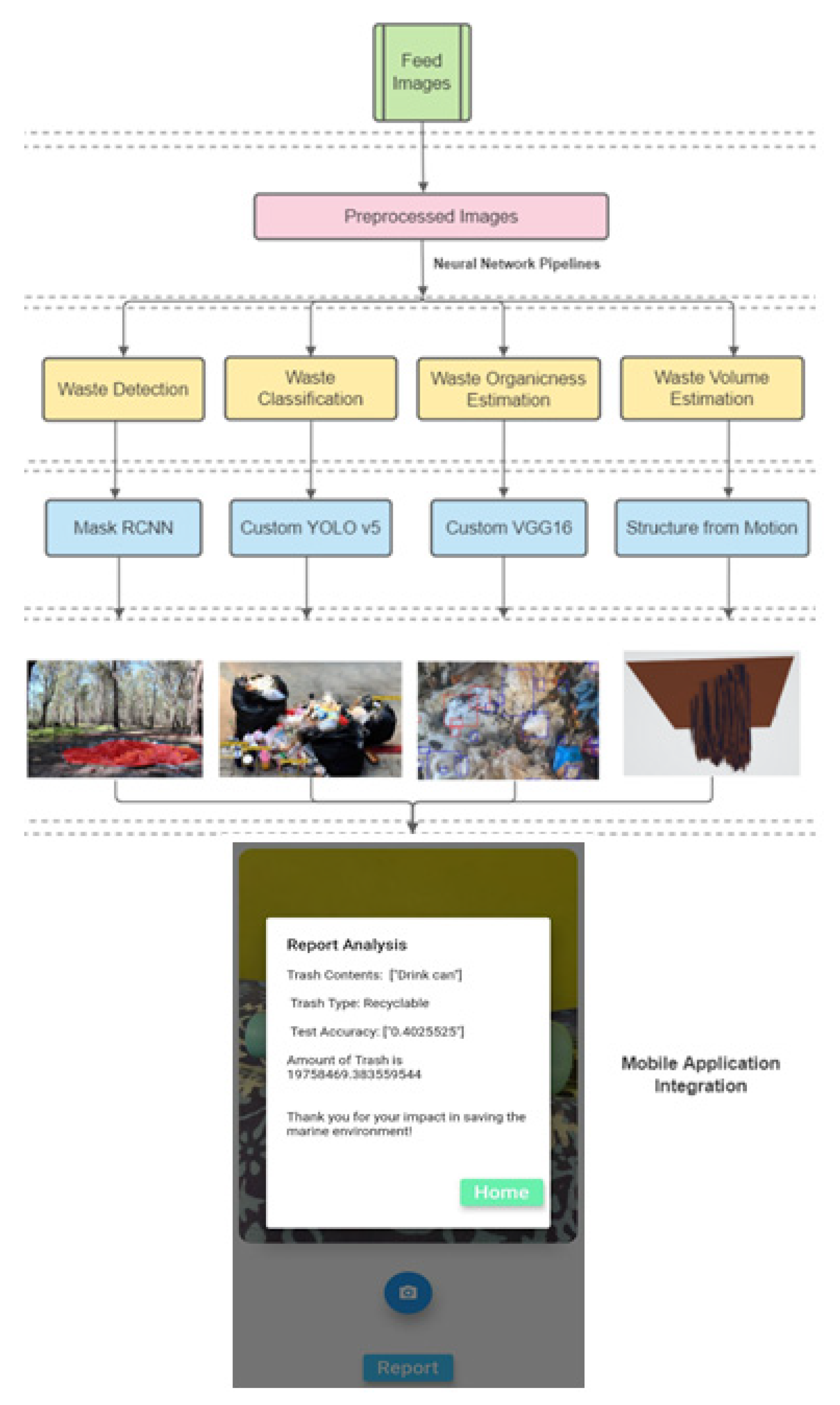
This section contains an analysis of the various ensembles of neural network pipelines involved in this research study. Figure 1 shows the schematic of the proposed framework for our waste management system. The input images are fed into the preprocessing network where normalization, flipping, subsetting, and cropping are performed. The preprocessed images are then passed onto the four neural network modules of waste detection, classification, volume calculation, and organic content estimation, using Mask Region-Based Convolutional Neural Network (RCNN) [15], You Only Look Once (YOLO) [6], Very Deep Convolutional Neural Network (VGG16) [24], and Structure from Motion (SFM) [25] models, respectively. All the modules function independently and are integrated into our fully functional mobile app.
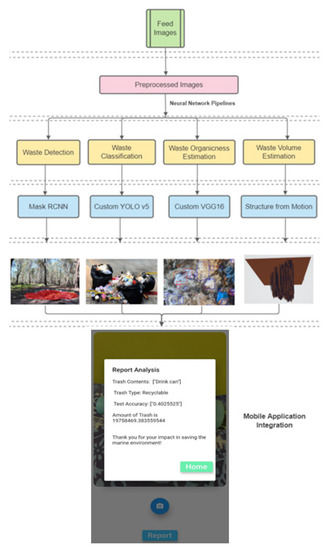
Figure 1.
Schematic of the proposed framework for the waste management system.
3.1. Data Preparation
To train the different neural network models for waste management, we combined two sets of recently released trash image datasets [5]. The datasets contain images of six different objects, namely plastic, metal, glass, paper, cardboard, and other organic trash. The conventional trash datasets do not consider the different organic waste that can be identified. Our model rectifies this issue and can classify trash accurately. Organic waste can be either an orange peel or hospital waste. We have included images of trash from various perspectives, as we cannot account for user behavior. The different angles and sizes of trash will enable a robust network and system for the neural pipeline to train and predict. There are 2527 labeled images in our dataset.
We ensure that none of the trash classes have any biases amongst themselves, thus allowing our neural network classification to achieve greater accuracy and address the issue of trash variance based on different user environments. The 2527 images are split into a 70:15:15 ratio for training, validation, and testing, respectively. The experimental setup was executed on an Ubuntu-based system with 16 GB RAM and 1 TB HDD storage with NVIDIA GeForce RTX 3090 as the primary GPU and tested on Python 3.7+ for the neural network models.
3.2. Waste Image Segmentation and Detection
The next important step was to perform waste detection and bounding box generation around the waste pile or litter object. Image segmentation was performed initially with Otsu image segmentation. Otsu thresholding was applied to the waste images for foreground and background separation to make the waste region more prominent for further analysis and implementation. Figure 2 is the resultant image after performing the Otsu method on an input image depicting a lineup of litter piles along bayside regions. Otsu’s methodology is a well-known technique for image segmentation which uses the threshold that minimizes the between-class variance. The threshold can be defined as the combined weighted total of the probability values of inter-class and intra-class calculated from the histogram bins, as shown in Figure 3.
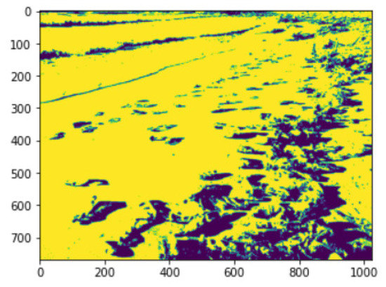
Figure 2.
Otsu’s segmentation output on waste in a coastal area.
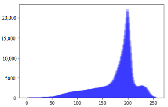
Figure 3.
Histogram of intensity for Otsu’s method.
The next step in image segmentation was edge thresholding, which was accomplished in our research using a multiscale LOG Detector, also known as the Marr–Hildreth Edge Detector. It makes use of a threshold value that keeps track of the multi-level intensity variation. Intensity variation results in a peak or a drop in the scaled graph. Gaussian and Laplacian filters are jointly convolved using a differential operator and scale fine-tuning. After convolution, the zero-crossing areas of the output image highlight the regions of intensity change. The sigma values were experimented with and tuned across Gaussian filters to obtain the highest optimal threshold value. The blurred image is convolved with the original image and then passed through a Laplacian filter, finally giving the output as shown in Figure 4.
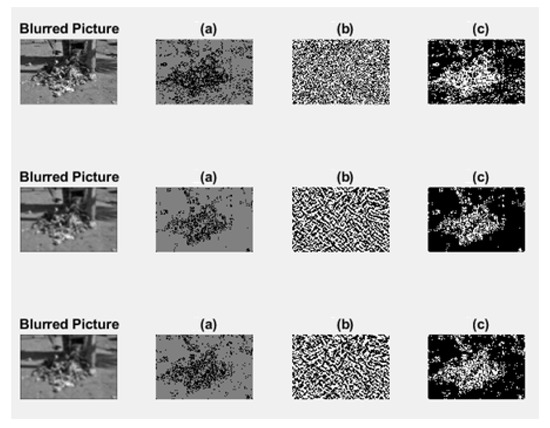
Figure 4.
LOG edge detector with 3 different level of sigma (3 rows). The blurred picture (column 1) obtained by applying the Gaussian filter on the original image, part (a) was obtained by applying Laplacian filter on the blurred image and display the positive values with the proper threshold and also in grayscale was next (b), and finally all the zero crossings are shown (c).
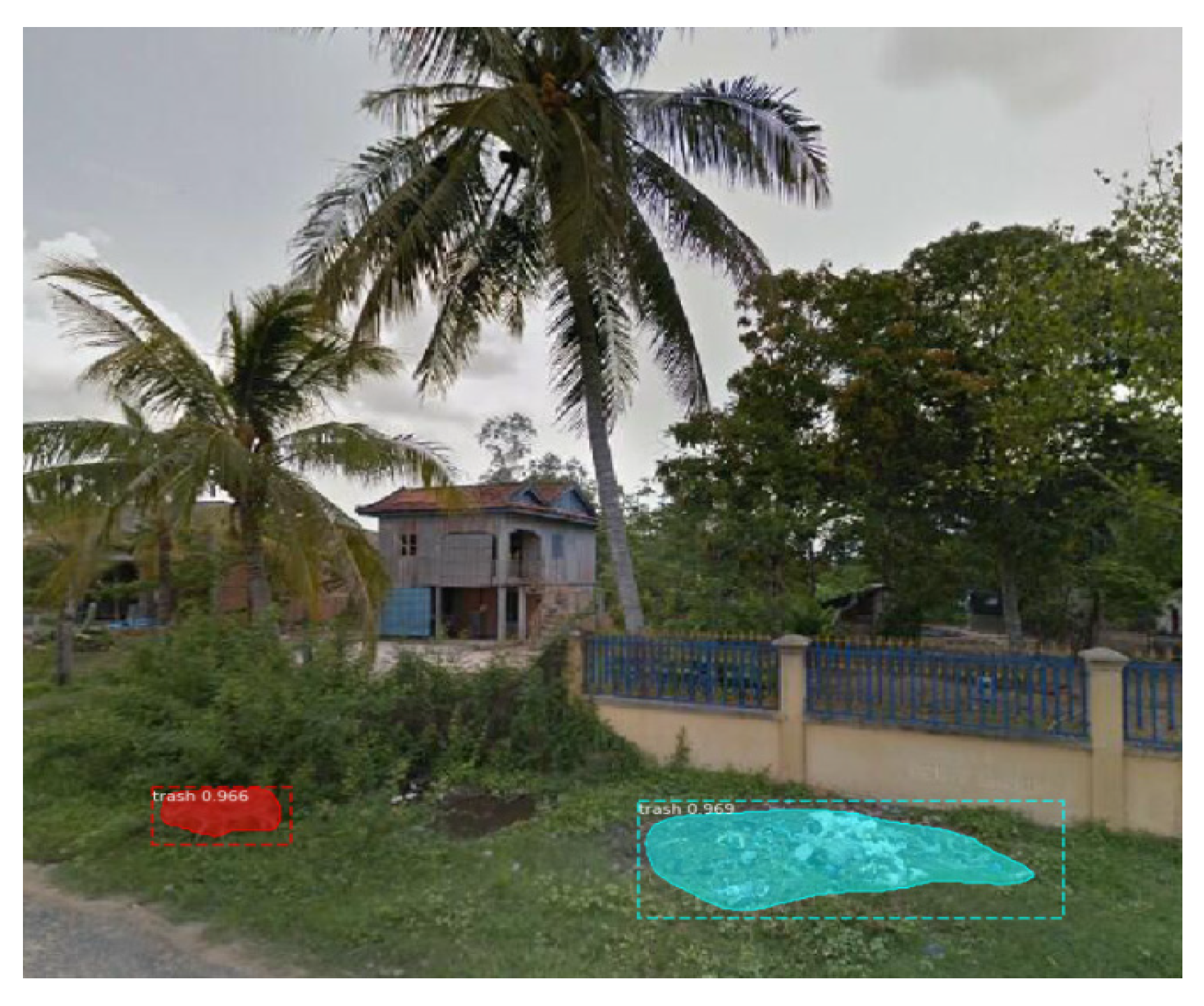
Finally, Mask RCNN is used for trash detection on images with the dimensions 1024 × 1024 × 3. Mask RCNN is used to automatically perform image segmentation and bounding box and contour identification, followed by object detection. This deep neural network architecture first generates a feature map for obtaining the region of interest in the image. It is then followed by mapping the proposed regions to object classes using ROIAlign. In our model, the learning rate of 0.001 and the learning momentum of 0.9 were used to train the data. A 28 × 28 mask was applied with a mask pool size of 14. The model was trained using 17 steps per epoch with a validation step count of 50 on 200 regions of interest for each image. The segmentation masks (visible as different colored sections) after applying Mask RCNN are displayed in Figure 5, Figure 6 and Figure 7, which accurately identify the waste pile location or individual trash in cases of no pileups. Figure 5 depicts a case where the detection is performed on a collective waste pile, in contrast to Figure 6, in which distributed waste piles are identified. To make the system more diversified, Figure 7 is a case where individual pieces of garbage are present. This makes our detection model more robust, incorporating various situations in which garbage can be identified in real time. The final accuracy of the Mack RCNN model was determined to be 92%, with an average loss of 0.452.
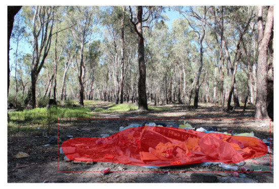
Figure 5.
Mask RCNN-based object detection on a waste pile.
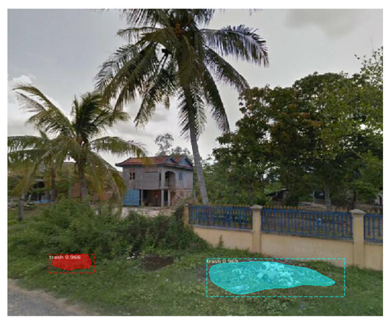
Figure 6.
Mask RCNN-based object detection on scattered litter.
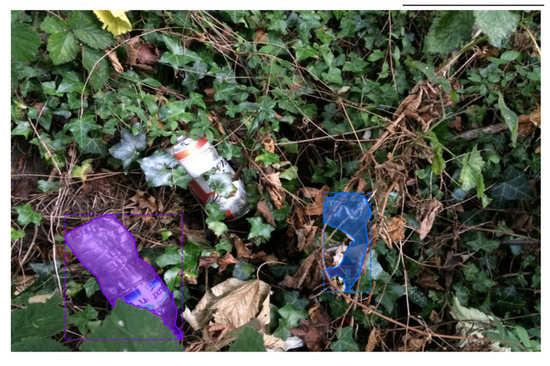
Figure 7.
Mask RCNN-based object detection on waste images from the TACO dataset.
3.3. Waste Classification and Real-Time Labeling
Waste classification is one of the most critical aspects of the proposed application. We primarily used the YoloV5 framework to carry out the whole prediction.
YOLO v5 is a novel, lightweight convolutional neural network (CNN) for real-time objects with improved accuracy. YOLO v5 makes use of a distinct neural network for single image processing. It is followed by separating images into segments and predicting bounding box coordinates and the probabilities for each segment. The expected probability is then used to weigh the detected bounding boxes. The method only has one forward propagation running through the neural network to make the predictions, followed by non-max suppression for the final prediction results.
The YOLO v5 architecture can be divided into three parts as follows:
- Backbone: The backbone is the key element for feature extraction given an input image. Robust and highly useful image characteristics can be extracted from an input image in this backbone layer using CSPNet (Cross Stage Partial Network), which is used as a backbone in YOLO v5.
- Neck: The neck is specifically used to create the feature pyramids, which are useful for object scaling. This is particularly useful for detecting objects of varied scales and sizes. PANet is used as the neck layer in YOLO v5 for obtaining the feature pyramids.
- Head: The model head is the final detection module. It makes use of anchor boxes for the construction of resultant output vectors with their classification scores, bounding boxes, and class probabilities.
The whole network is a combination of an ensemble system, with several learners comprising the backbone network, neck, and the head of the neural network system. The image first goes into a custom neural network and is primarily resized into 608 × 608 pixel resolution. It is essential that the resolution is of optimal quality and accuracy, which can be easily found in most handheld devices. The network itself makes the image compatible for further processing. The image is color plane separated and passed into the ensemble pipeline. One of the neural network parts has an architecture of six convolutional layers and max pooling blocks, obtaining valuable pieces of information from every layer. The max pooling layer plays a crucial role in reducing the pixel information at every successive layer, making it suitable for the convergence to be further used by the YOLO network in the next part of the network. In this part of the neural pipeline, the pixelated image’s first stage passes through the 53 Darknet layers, acting as the additional feature detector with the last part of the network. The previous features and the currently identified ones comprise the backbone of the network, enhancing the accuracy of correct detection. This is a typical example of deep transfer learning. Simultaneously, another parallel pipeline executes the same 608 × 608 pixel image using a different procedure.
The three losses, Loss1, Loss2, and Loss3, are the box, classification, and objectness losses, respectively. The box loss represents how perfectly the algorithm can locate the object center and how well the predicted bounding box covers an object. Classification loss measures the accuracy of correct class prediction by the algorithm. Objectness is essentially a probability measure of the existence of an object in a proposed region of interest. The higher the objectivity, the greater the likelihood of a window to contain the object.
where hi, wi, xi, yi are the height, width, and centroid coordinate, respectively, of the specific anchor box. The aggregate TotalLoss function is calculated by summing up Loss1, Loss2, and Loss3. ci is the resultant computed confidence score of object pi(c) which pertains to the classification loss. The parameters with hats correspond to the estimated values. c denotes the respective classes. εobjij is 1 only when there is an object in the grid cell and 0 in all other cases.
Total loss = Loss1 + Loss2 + Loss3
βcrd = 10 × βnobj
βnobj = 0.5
βcrd = 6
εobjij = depicts the j-th bounding box in the grid cell i
εnobjij = −εobjij
The second learner primarily uses the EfficientNet network. It is a more careful network than the previous neural pipeline. EfficientNet balances the network width and depth and optimizes the image resolution for better accuracy. It contains a mixture of convolutions and mobile inverted convolutions. This system in practice has excelled over other famous networks. After both pipelines—or, in ensemble terms, learners—have processed all the convolutions, it is passed into a decider, which considers each system’s flaws. If one of the pipelines misses any important feature, the decider changes the weight accordingly. After several iterations of this process, the decider converges into a standard weight value, detecting the correct features of the trash images in a scene image. Initially, InceptionV3 was also incorporated in this pipeline, but unfortunately, the pipeline acted as an inhibitor in the current neural network and decreased the accuracy. Thus, after the decision and a series of forwarding and backward propagation, a feature map of 7 × 7 × 256 was the result of the entire system. There was appreciable downsampling in the image structure. The final part of the network was passed into a wide range of further convolutions to result in 7 × 7 × 21 pixel resolution. This was carried out to convert a two-dimensional tensor into a three-dimensional tensor to establish clear bounding boxes.
The last part of the YOLO framework now comes into play—as compared to the previous part, which acted as the feature detector added with the EfficientNet additional rectified features—wherein the weights are passed into the object detector part of the YoloV5 framework. The successive 53 layers allow widespread object detection of small, medium, and large sizes. This is crucial, as the user might supply an image of a trash pile with a variable distance. The object detector is efficient enough to categorize a variety of trash types from a pile with an accuracy of 93.65%. Thus, there are several fully connected layers at the end of the network, and finally, the total number of possible classification classes in the data. The bounding boxes created by the network are exact in creating the blobs and generating the labels classified in real time, as per the final deciding output of the entire network, depicted in Figure 8. The model has been trained to identify recyclable waste items from a trash pile in this figure. The network outputs bounding boxes with the class identified and their confidence scores. The MobileNetv3 and Detectron2 models were also tested for the waste classification module to compare the models in search of selecting the best one. MobileNet V3 is ideally tuned for mobile devices, which is appropriate for the use case of this research. It internally uses AutoML and leverages two primary techniques, i.e., MnasNet and NetAdapt. It first searches for a coarse architecture using the former, applying reinforcement learning to choose an optimal configuration. The latter technique primarily fine-tuned the model, trimming the underutilized network activation channels by using small decrementing steps in every iteration. Detectron2 is an imposing network model. It comprises a backbone network that consists of Base-RCNN-FPN network features. It is tasked to extract the feature maps efficiently and comprehensively. The next part of the network is the region proposal subnetwork that detects object regions from multiscale features. The final part is the box head component, which warps and crops the feature maps accompanied by the previous component and obtains fine-tuned boxes locating the region and object of interest.
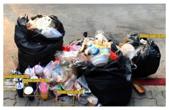
Figure 8.
Waste detection from pile using YOLO.
3.4. Organic Waste Estimation
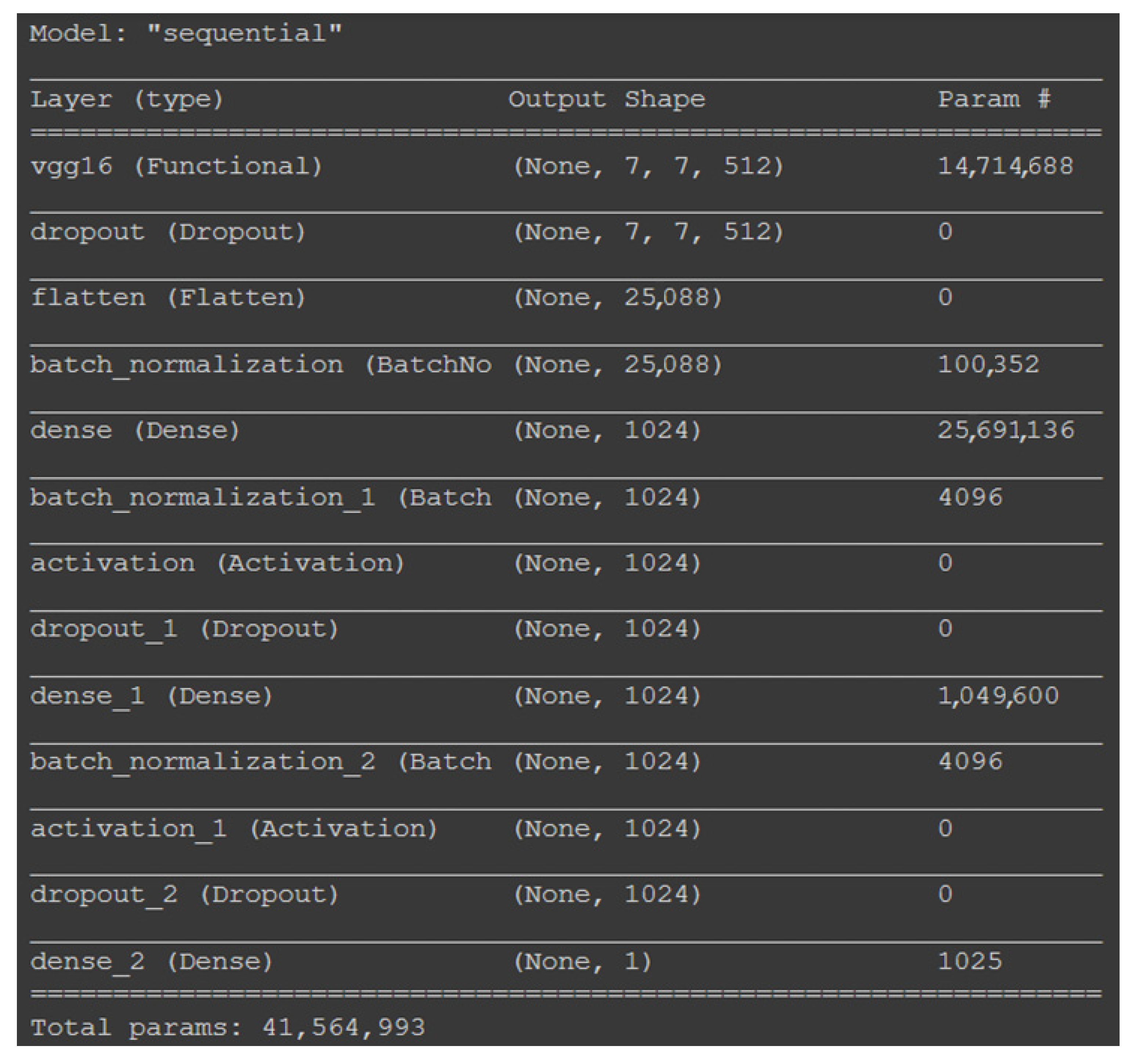
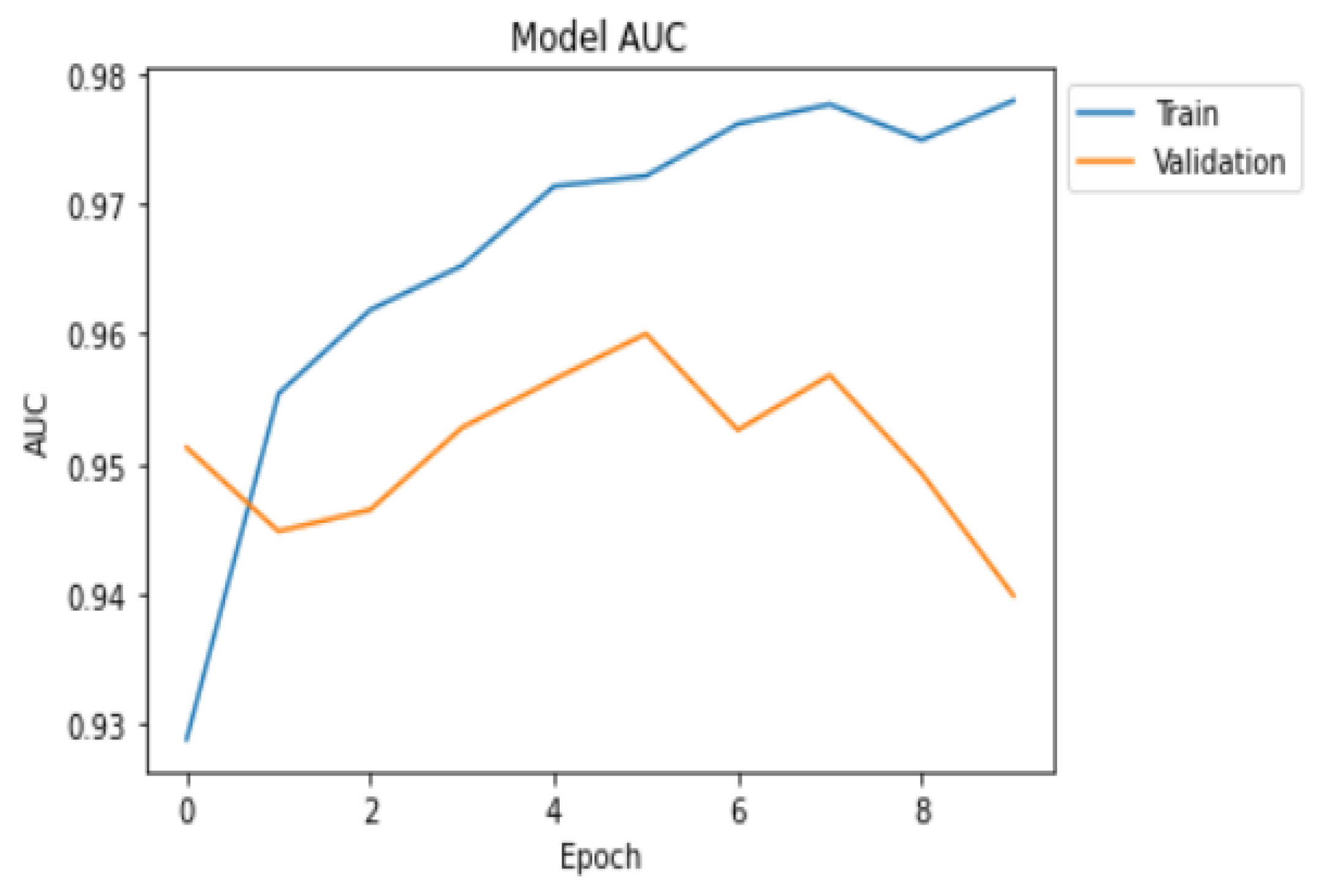
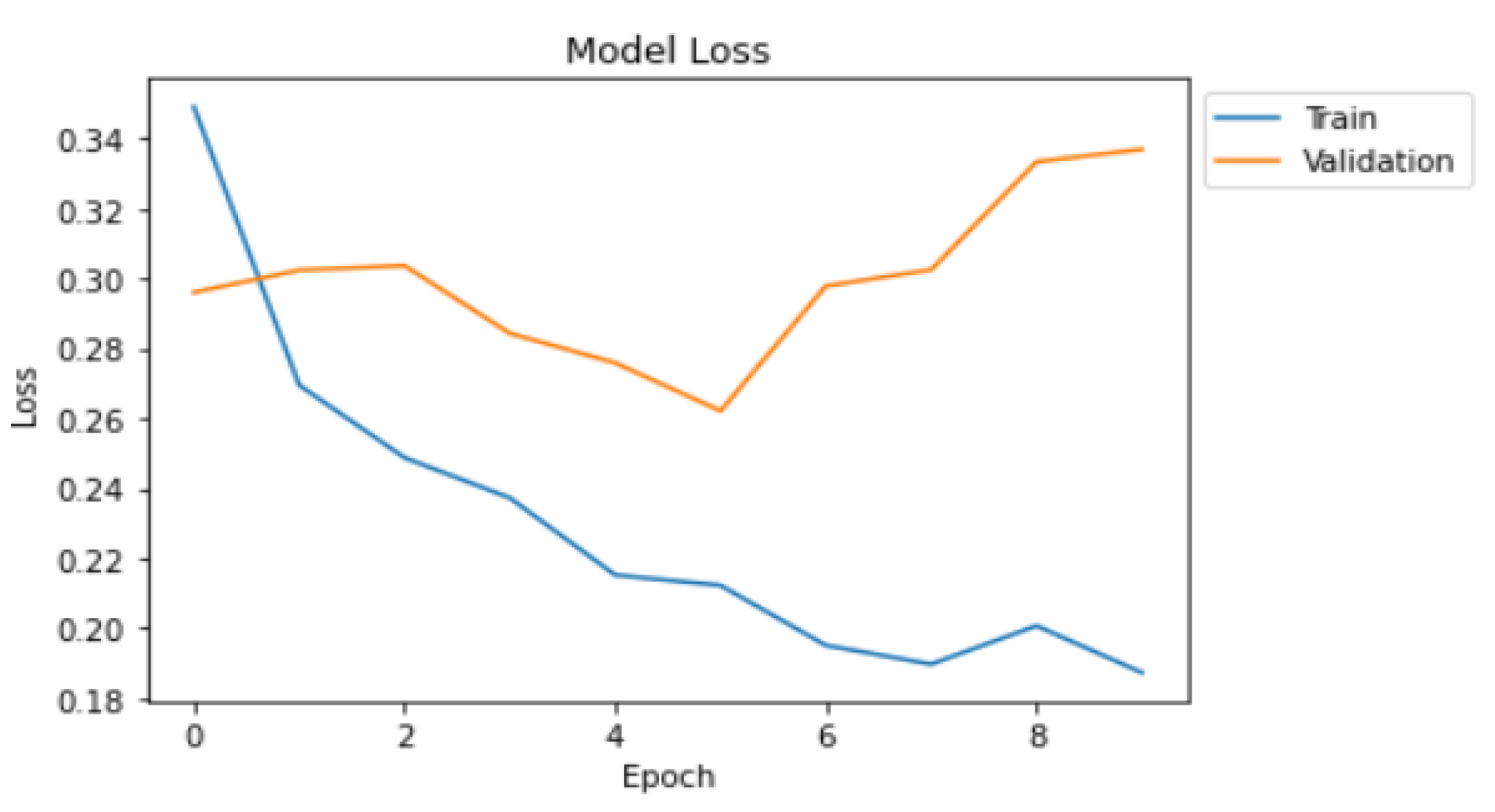
Waste management is an important problem worldwide. In addition, estimation, and classification of waste as organic and recyclable is another important factor that is difficult to annotate manually. The approach used in the paper applied a convolutional neural network model to a household waste dataset consisting of 22,500 training samples, split into 18,000 images for training and 4500 images for validation. VGG16 network architecture is used as a base for model training. The model architecture is shown below in Figure 9. The network feeds in an input shape of (7, 7, 512), where the last index is the number of input channels. Transfer learning has been implemented in this network by incorporating one flattened layer and three dense, normalization, dropout, and activation layers, consisting of a total of 41,564,993 trainable parameters. The model was then compiled with binary cross-entropy loss and OPT optimizer. The results were impressive, with loss and AUC metrics of 0.184 and 0.9779, respectively, and validation loss and AUC of 0.33 and 0.9399, respectively. The accuracy of validation data was 95.60%, and the accuracy of test data was 94.98%.
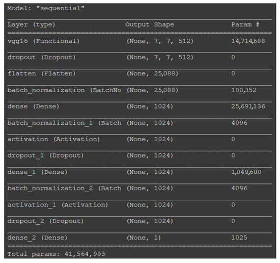
Figure 9.
Model architecture.
The images were successfully separated into recyclable and organic waste categories. In the application, the class would be prompted to the cleaner along with the waste geotagged location and volumetric content.
3.5. Volumetric Analysis of Waste Using STL and Point Cloud Models via SFM
The volumetric analysis of the waste pile was an essential integration into the research. The Structure from Motion (SFM) approach was used in modeling the 2D to the 3D reconstruction of the waste pile. The research considered the possibility of waste in a pile format or even as scattered litter. If a waste pile is detected, the user would be prompted to take a short video clip of the waste pile with a 360-degree view. Our model would then capture 100 frames from the video clip and use the captured frames in the SFM module. SFM is a crucial 2D to 3D reconstruction technique that uses a series of frames or images and aims to reconstruct a 3D view of the object. Point clouds are used in SFM for generating the 3D model. Another important reason for selecting the SFM model was its minor dependency on high-resolution camera equipment. Simple day-to-day smartphone cameras can be easily used to capture images fed into our SFM model. If the images have a certain overlapping degree, the SFM model yields accurate results, and this is ensured by the user-shot, 360-degree video of the waste pile. The first stage of SFM is matching the image features using SIFT or SURF methods and estimating the distance between them. It is followed by the important stage of understanding our structures by calculating the camera positions and orientations.
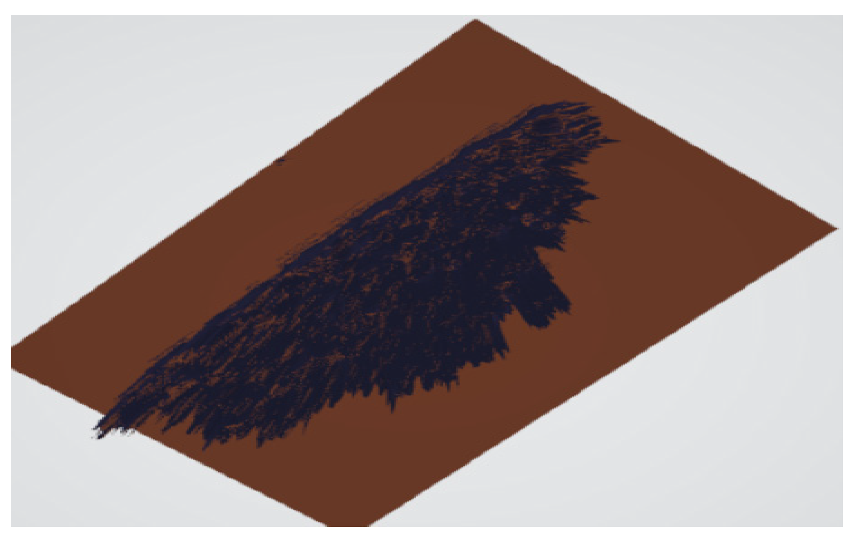
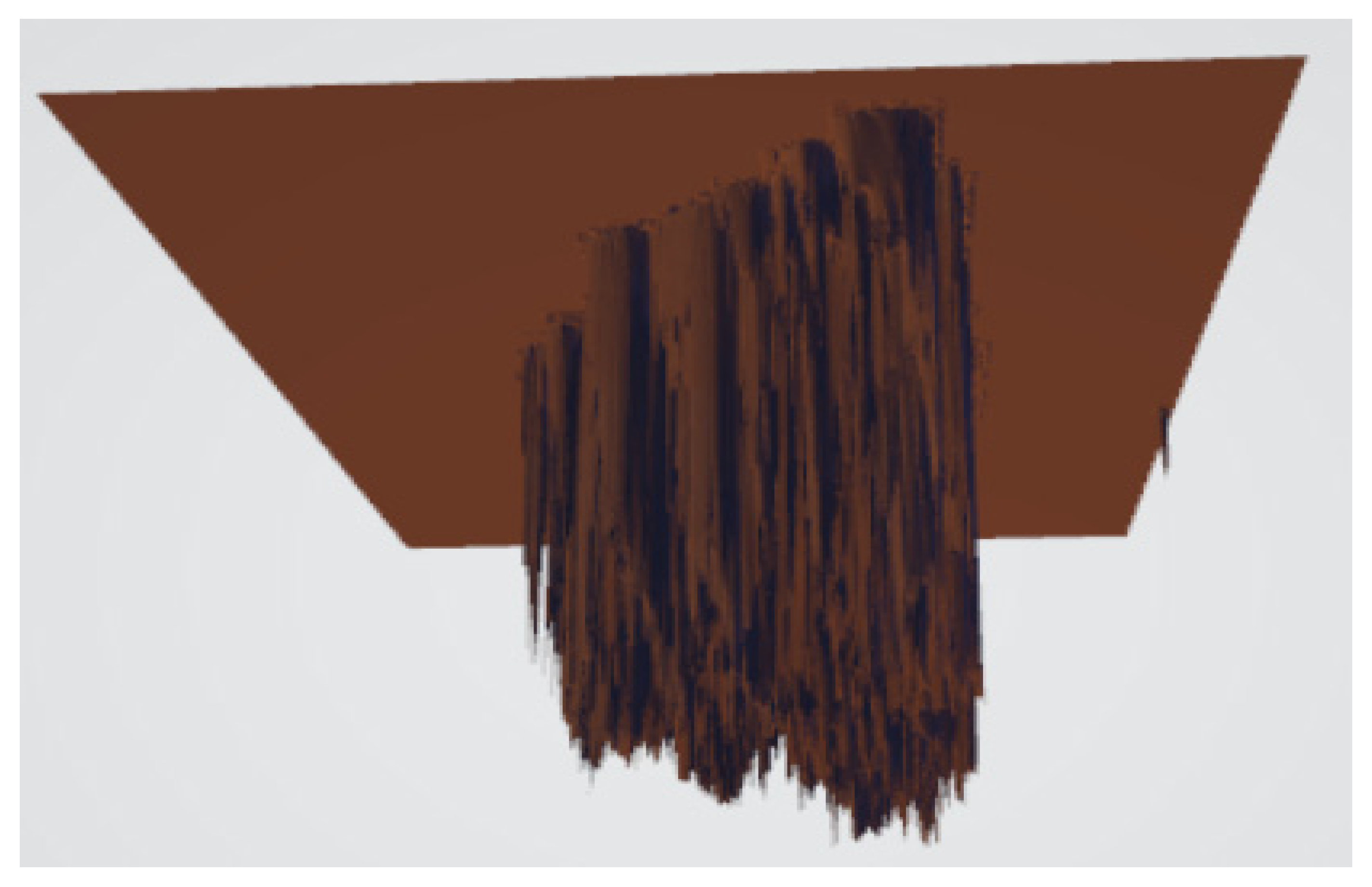
The image features and parameters are related to the scene structure, whereas the camera positions are referred to as motion; hence, the term “Structure from Motion” was coined. A point cloud is essentially a collection of data points in three-dimensional space. Figure 10 creates a point cloud representation of a trash pile. Since volume is an essential morphological characteristic of an object, having an idea of the volume estimation using point cloud structures is key. This 3D surface construction uses dense point cloud structure generation in Figure 11 and Figure 12. The point cloud generated from SFM methodology is uniquely used in our work for volume estimation. The edge points of the top-most and bottom-most pixels of the generated point cloud were measured to approximate the height of the waste pile. The height obtained was fed into our STL and Trimesh model. A conical mesh was created and stored in STL format, serving as our image mask. Using the Pillow Python library, one of the waste pile images was read, and after surface construction (Figure 11 and Figure 12) and plugging in the height value, the Python Trimesh library was used for volume estimation of the waste pile, as shown in Figure 13. The volumetric estimation pipeline had an accuracy of 85.3%.
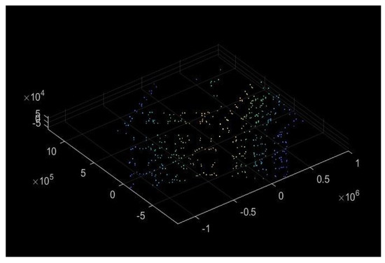
Figure 10.
Point cloud generation of a waste pile.

Figure 11.
Waste pile reconstructed.
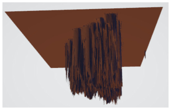
Figure 12.
Waste pile 3D constructed using STL.

Figure 13.
Volume estimation using Trimesh on the STL file.
3.6. WDCVA App Module Integration
Each application user can be distinguished into three categories: admin, worker, and citizen. The user must first log in or sign-up using phone number authentication, regardless of the user type. The phone authentication is powered by Firebase Authentication, which validates the phone number and returns an OTP to verify the user. Apart from the phone number, the user must submit personal information including name, age, and gender. All this information will be stored in Firestore as specific user documents. These documents are used to categorize the user into the above-mentioned types. Hence, when logging in, if the phone number is found in the database, the app displays information according to the user type.
For citizens, the landing page displays a dashboard where the user can track the progress of the reports submitted earlier. This would provide transparency and support the motive for submitting more reports. There is also a quick access floating button, allowing citizens to make a quick report. When the button is pressed, the application will display a screen where the user can capture a picture of the litter whose report needs to be submitted. The application allows the image to be taken from the phone storage or captured through the camera. After the image is decided, the app previews the chosen image. Once the citizen is satisfied with the image, the citizen can report the litter. When the button is pressed, the user’s geolocation is also tagged with the report, enabling workers to find the litter. The report details are submitted to a custom Flask API, which analyzes the submitted image at the backend. The same analysis is returned to the citizen as proof of submission.
The reports are stored separately on Firestore as documents and displayed in the user interface, as shown in Figure 14, comprising the identified trash contents, the type of garbage identified, and the confidence accuracy. It also depicts the volume calculated for the current localized garbage in the image. Apart from containing the location and picture of the litter, the report document also contains a status field, which can hold the values of pending, in progress, and cleaned. This allows tracking of the litter cleaning process.
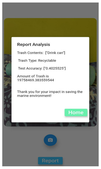
Figure 14.
Mobile app trash analysis report.
For workers, the dashboard displays a map with pins that signify the locations with litter reports that are still pending. The workers can choose the reports closest to them and start cleaning those locations. When the worker has started the process, it is the worker’s responsibility to mark the report as “in progress” when the work has started and then as “cleaned” upon completion.
4. Results and Discussion
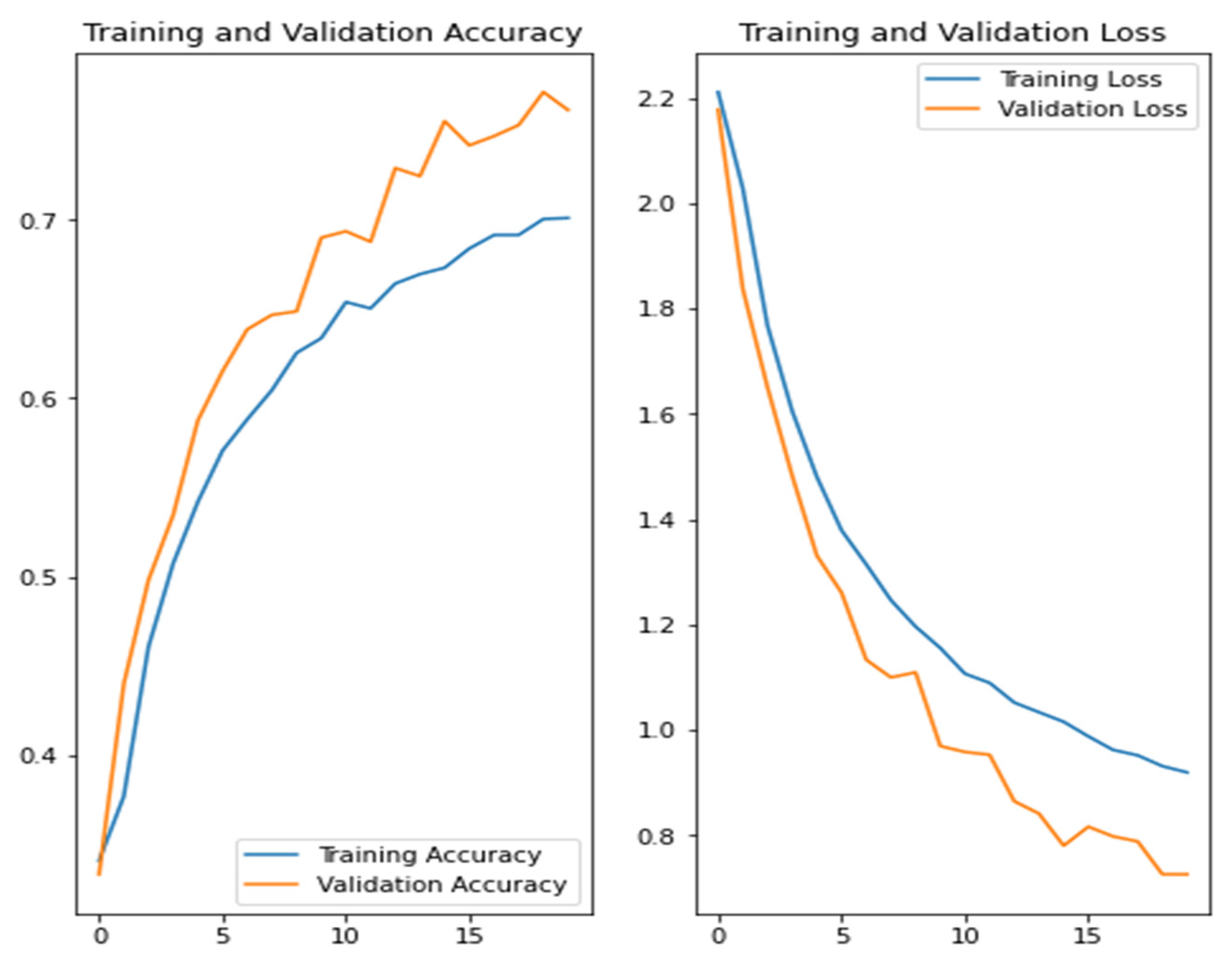
The object detection model was made more robust and accurate using image thresholding and segmentation techniques such as Otsu’s thresholding and LOG edge detectors. The Mask RCNN accurately identified the blob of a waste pile or even scattered data. The trash classification was successfully executed by the proposed ensemble pipeline and achieved an accuracy of about 93.65%. The waste classification on untrained images, along with various changes in orientation and agglomerated trash in piles, were all accounted for precisely. With the EfficientNet learners, the YOLO backbone framework resulted in a real-time trash classification pipeline. Figure 15 depicts the training and validation accuracy and losses for the YOLO v5 model. The model validation accuracy stands at 93.65%, and the model training accuracy is 88.92%. The training and validation losses amount to 0.585 and 0.492, respectively. Learning curves are useful for extracting meaningful information regarding a model’s overfitting, underfitting, and well-fitting. Hence, we compared the learning curves of the top two algorithms used in our research, namely YOLO v5 and MobileNet v3. As is evident from Figure 15, the losses start with high values, reduce over time with training steps, and reach close to stabilization. The accuracy score of validation and testing also increases with increasing training steps, which hints at a moderately well-fitted model. The higher validation accuracy and lesser validation losses might lead to overfitting concerns, but this can be controlled with the dropout layer values. The testing and validation accuracies of the MobileNet architecture are plotted in Figure 16. The losses in Figure 16 still have a chance to saturate, and hence the model shows some underfitting, and the accuracy scores are lower compared to Figure 15 of the YOLO v5 model.
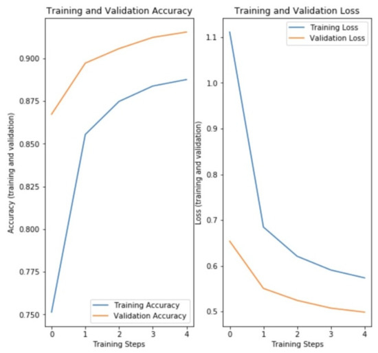
Figure 15.
Training and validation accuracy for YOLO v5 architecture.
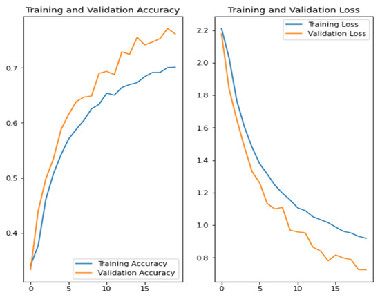
Figure 16.
Training and validation accuracy for MobileNet architecture.
The volumetric model using SFM generated accurate point cloud structures for the waste pile, which accurately gave the edge points of the pile and hence the probable height of the pile. The STL and Trimesh Python libraries yielded volume estimation using STL files generated by the detected waste pile. The organic and recyclable waste model gave an impressive accuracy of 95.6%, which is also a vital waste management metric aimed at helping protect the environment. Since the litter reports submitted by the citizens also contain the geolocation of the litter, with enough data collected, the litter can be easily traced to the source, thus allowing litter dumping at the source. The map for workers will improve the time to clean the litter locations because previously, the workers were generally unaware of where to search for litter.
Precision measures the accuracy of our predictions; particularly what percentage of our predictions are correct. The denominator is a descriptor of the predictions in the analysis.
TP = True positives (predicted as positive and are correct)
FP = False positives (predicted as positive but are incorrect)
Recall calculates how well we can find the positives. For instance, we can find 70% of the possible positive results in our top K predicted results. Here, the denominator evaluator of the ground truths is involved in the analysis.
TP = True positives (predicted as positive and are correct)
FN = False negatives (an object that was there but not predicted)
mAP is a popular evaluation metric in computer vision that can be used for object localization and classification. It stands for mean average precision. mAP is averaged over average precision (AP). AP is the summation of the difference between the kth and (k − 1)th recall, multiplied with the kth precision for n number of thresholds.
Table 1 depicts the abovementioned evaluation metrics for various models such as the custom YOLO v5 and MobileNet V3, tested for waste classification. Each model was run for 100 epochs on NVIDIA GeForce RTX 3090 as the primary GPU. We chose YOLO v5 as our primary model because of its higher accuracy and mAP values as well as lower latency and more lightweight structure than other models, as shown in Table 1. The model is smaller and far better at detecting smaller objects. Although the speed measured in frames per second (fps) is almost similar for YOLO v5 and MobileNet v3, the accuracy is the main underlying factor for final model consideration, and this has shown to be greater for our dataset using the YOLO v5 model.

Table 1.
Evaluation metrics of different models tested for waste classification.
Below, we present a comparison between our work and the existing works in this domain with the help of Table 2 and Table 3. The existing works target specific use cases such as singular waste segmentation, classification, or volume estimation. First, in Table 2, we added our use cases as separate modules and the model used and its overall accuracy. In Table 3, we present the use cases of the existing research work mentioned in the literature survey section, their methodology or model used, and their overall accuracy scores.

Table 2.
Performance evaluation of the proposed model.

Table 3.
Performance comparison of the proposed model with existing models.
Since we also used CNN models in the organic content estimation module, we have plotted the area under curve (AUC) plot and loss plots. The graphs and metrics for the waste organic estimation module are shown in Figure 17 and Figure 18. The training loss decreased over each epoch, but the validation loss increased after epoch 5, which shows overfitting; hence, we trained our model for four epochs to achieve the best accuracy.
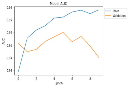
Figure 17.
Area under curve performance of the proposed model.
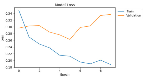
Figure 18.
Loss curve of the proposed model.
5. Conclusions and Future Work
Waste management is an important factor in environmental monitoring. Moreover, our proposed model comprising waste detection, classification, organic waste identification, and volumetric analysis of waste piles is a unique approach towards developing a smart waste management system. In this paper, a comprehensive review of existing research works with their use cases, models, and accuracy is highlighted. Furthermore, we performed a comparison of implemented models and our proposed model. The models used are supported with appropriate evaluation curves and metrics to understand their performance and to pave the way for future improvements. In contrast to the traditional methods of manual monitoring and management of waste, which require manual labor and suffer from lack of access to specific geographic locations and classification challenges, our research work using AI and deep learning can harness accurate and efficient waste management.
Our work invites several areas to be explored further, such as real-time waste detection based on a video feed. One of our key future works would be to explore volume estimation and waste identification based on real-time video input and to apply state-of-the-art algorithms such as RetinaTrack [27] or Tracktor++ [28] to achieve accurate predictions. Real-time 360 views from video images can also help generate a more real-life waste pile structure and, in turn, might lead to more robust volume estimations. It would also help address the issue of the liveliness of waste detection, i.e., not identifying a waste pile drawn on paper or shown on a digital screen as a waste pile. There also lies a future extension of bringing in the concept of carbon credits into our mobile app so that carbon footprints can be reduced by providing incentives to our app users, thus giving our app and research a more beneficial outcome in society.
We derived several crucial managerial insights from this research study. The primary derivations are the need for a mobile-based app for effective and smart waste management in contemporary society. With the help of cutting-edge AI and DL algorithms, the predictions and results can be made more accurate and relevant, which are important aspects of the work presented. The study also aims to reduce the carbon footprint by optimizing and precisely pinpointing identified trash locations. Another major motive of this paper is an attempt to identify the category of waste for proper processing and to reduce biodegradable-non biodegradable waste mix-up, which is a rising concern. We also aim to give an opportunity to provide a scope of analysis to estimate the ratio between identified and recycled volumes of waste.
Author Contributions
Conceptualization, S.G. and J.S.; methodology, I.D.; software, R.B.; validation, S.G., J.S., I.D., R.B. and S.K.; formal analysis, S.K. and I.A.L. All authors have read and agreed to the published version of the manuscript.
Funding
This research received no external funding.
Institutional Review Board Statement
Not applicable.
Informed Consent Statement
Not applicable.
Data Availability Statement
Not applicable.
Conflicts of Interest
The authors declare no conflict of interest.
References
- Beliën, J.; De Boeck, L.; Van Ackere, J. Municipal Solid Waste Collection and Management Problems: A Literature Review. Transp. Sci. 2014, 48, 78–102. [Google Scholar] [CrossRef]
- Hiremath, S.S. Population Growth and Solid Waste Disposal: A burning Problem in the Indian Cities. Indian Streams Res. J. 2016, 6, 141–147. [Google Scholar]
- Halkos, G.; Petrou, K.N. Efficient Waste Management Practices: A Review; MPRA, University Library of Munich: Munich, Germany, 2016; Available online: https://mpra.ub.uni-muenchen.de/71518/1/MPRA_paper_71518.pdf (accessed on 24 December 2021).
- Henrys, K. Mobile application model for solid waste collection management. SSRN Electron. J. 2021, 20, 1–20. [Google Scholar] [CrossRef]
- Mittal, G.; Yagnik, K.B.; Garg, M.; Krishnan, N.C. SpotGarbage: Smartphone app to detect garbage using deep learning. In Proceedings of the 2016 ACM International Joint Conference on Pervasive and Ubiquitous Computing (UbiComp ’16), Heidelberg, Germany, 12–16 September 2016; ACM: New York, NY, USA, 2016; pp. 940–945. [Google Scholar] [CrossRef]
- Redmon, J.; Divvala, S.; Girshick, R.; Farhadi, A. You only look once: Unified, real-time object detection. In Proceedings of the IEEE Conference on Computer Vision and Pattern Recognition, Las Vegas, NV, USA, 27–30 June 2016; pp. 779–788. [Google Scholar]
- Xu, Z.; Xu, C.; Hu, J.; Meng, Z. Robust resistance to noise and outliers: Screened Poisson Surface Reconstruction using adaptive kernel density estimation. Comput. Graph. 2021, 97, 19–27. [Google Scholar] [CrossRef]
- Rusu, R.; Cousins, S. 3D is here: Point Cloud Library (PCL). In Proceedings of the 2011 IEEE International Conference on Robotics and Automation, Shanghai, China, 9–13 May 2011. [Google Scholar]
- Vishnu, S.; Ramson, S.; Senith, S.; Anagnostopoulos, T.; Abu-Mahfouz, A.; Fan, X.; Srinivasan, S.; Kirubaraj, A. IoT-Enabled Solid Waste Management in Smart Cities. Smart Cities 2021, 4, 53. [Google Scholar] [CrossRef]
- Xia, W.; Jiang, Y.; Chen, X.; Zhao, R. Application of machine learning algorithms in municipal solid waste management: A mini review. Waste Manag. Res. 2021. [Google Scholar] [CrossRef] [PubMed]
- Kraft, M.; Piechocki, M.; Ptak, B.; Walas, K. Autonomous, Onboard Vision-Based Trash and Litter Detection in Low Altitude Aerial Images Collected by an Unmanned Aerial Vehicle. Remote Sens. 2021, 13, 965. [Google Scholar] [CrossRef]
- Fulton, M.; Hong, J.; Islam, M.; Sattar, J. Robotic Detection of Marine Litter Using Deep Visual Detection Models. In Proceedings of the 2019 International Conference on Robotics and Automation (ICRA), Montreal, QC, Canada, 20–24 May 2019. [Google Scholar]
- Chu, Y.; Huang, C.; Xie, X.; Tan, B.; Kamal, S.; Xiong, X. Multilayer Hybrid Deep-Learning Method for Waste Classification and Recycling. Comput. Intell. Neurosci. 2018, 2018, 1–9. [Google Scholar] [CrossRef] [PubMed] [Green Version]
- Wang, T.; Cai, Y.; Liang, L.; Ye, D. A Multi-Level Approach to Waste Object Segmentation. Sensors 2020, 20, 3816. [Google Scholar] [CrossRef] [PubMed]
- Hong, J.; Fulton, M.; Sattar, J. TrashCan: A Semantically Segmented Dataset towards Visual Detection of Marine Debris. 2020. Available online: https://arxiv.org/abs/2007.08097 (accessed on 24 December 2021).
- Carolis, B.; Ladogana, F.; Macchiarulo, N. YOLO TrashNet: Garbage Detection in Video Streams. In Proceedings of the 2020 IEEE Conference on Evolving and Adaptive Intelligent Systems (EAIS), Bari, Italy, 27–29 May 2020. [Google Scholar] [CrossRef]
- Mohbat, T.; Abdul, W.A.; Mohammad, M.; Murtaza, T. Attention Neural Network for Trash Detection on Water Channels. 2020. Available online: https://arxiv.org/abs/2007.04639 (accessed on 24 December 2021).
- Majchrowska, S.; Mikołajczyk, A.; Ferlin, M.; Klawikowska, Z.; Plantykow, M.; Kwasigroch, A.; Majek, K. Deep learning-based waste detection in natural and urban environments. Waste Manag. 2022, 138, 274–284. [Google Scholar] [CrossRef] [PubMed]
- Chen, J.; Mao, J.; Thiel, C.; Wang, Y. iWaste: Video-Based Medical Waste Detection and Classification. In Proceedings of the 2020 42nd Annual International Conference of The IEEE Engineering in Medicine & Biology Society (EMBC), Montreal, QC, Canada, 20–24 July 2020. [Google Scholar] [CrossRef]
- Ruiz, V.; Sánchez, Á.; Vélez, J.; Raducanu, B. Automatic Image-Based Waste Classification. From Bioinspired Systems and Biomedical Applications to Machine Learning; Springer International Publishing: Cham, Switzerland, 2019; pp. 422–431. [Google Scholar]
- Vo, A.; Hoang Son, L.; Vo, M.; Le, T. A Novel Framework for Trash Classification Using Deep Transfer Learning. IEEE Access 2019, 7, 178631–178639. [Google Scholar] [CrossRef]
- Nilopherjan, N.; Piriyadharisini, G.; Rajmohan, R.; Sandhya, S.G. Automatic Garbage Volume Estimation Using Sift Features Through Deep Neural Networks and Poisson Surface Reconstruction. Int. J. Pure Appl. Math. 2018, 119, 1101–1107. [Google Scholar]
- Suresh, S.; Sharma, T.; Sitaram, D. Towards quantifying the amount of uncollected garbage through image analysis. In Proceedings of the Tenth Indian Conference on Computer Vision, Graphics and Image Processing—ICVGIP’16, Guwahati Assam, India, 18–22 December 2016. [Google Scholar] [CrossRef]
- Simonyan, K.; Zisserman, A. Very deep convolutional networks for large-scale image recognition. In Proceedings of the ICLR, San Diego, CA, USA, 7–9 May 2015. [Google Scholar]
- Özyeşil, O.; Voroninski, V.; Basri, R.; Singer, A. A survey of structure from motion. Acta Numer. 2017, 26, 305–364. [Google Scholar] [CrossRef]
- Godard, C.; Mac Aodha, O.; Brostow, G.J. Unsupervised Monocular Depth Estimation with Left-Right Consistency|UCL Visual Computing. 2021. Available online: http://visual.cs.ucl.ac.uk/pubs/monoDepth/ (accessed on 16 May 2021).
- Lu, Z.; Rathod, V.; Votel, R.; Huang, J. RetinaTrack: Online Single Stage Joint Detection and Tracking. In Proceedings of the IEEE/CVF Conference on Computer Vision and Pattern Recognition (CVPR), Seattle, WA, USA, 13–19 June 2020. [Google Scholar]
- Bergmann, P.; Meinhardt, T.; Leal-Taixe, L. Tracking without bells and whistles. In Proceedings of the IEEE International Conference on Computer Vision (ICCV), Seoul, Korea, 27 October–2 November 2019. [Google Scholar]
Publisher’s Note: MDPI stays neutral with regard to jurisdictional claims in published maps and institutional affiliations. |
© 2022 by the authors. Licensee MDPI, Basel, Switzerland. This article is an open access article distributed under the terms and conditions of the Creative Commons Attribution (CC BY) license (https://creativecommons.org/licenses/by/4.0/).

