Modeling of Reverse Curves on a Railway Line Using the Analytical Design Method

Abstract

This study discusses the issue of designing reverse curves, i.e. a geometric system consisting of two circular arcs (usually with different radii), directed in opposite directions and directly connected to each other. The design is performed in an appropriate local Cartesian coordinate system. The origin of this system is located at the point of intersection of adjacent main directions of the route. Unlike other geometric situations, reverse curves have three main directions, which significantly complicate the design process. The initial values of the radii of the reverse arcs must correspond to the existing system of main directions. The introduction of transition curves causes these radii to decrease; their values are determined iteratively. A set of formulas for creating a geometric system of reverse curves is presented. These formulas were used in the calculation example. A graph of the horizontal curvature of the track axis and a method for determining the possible train speed, both without the use of cant on an arc and with the use of cant, are shown. The presented procedure is universal and can be applied to other geometric situations involving the design of reverse curves. It is also necessary to emphasize the practical usefulness of the discussed method not only in the design process, but also to pay attention to the cognitive value of the article.

1. Introduction

In the field of railways, numerous research works are currently being carried out, among which the following can be distinguished: high-speed railways (e.g., [1,2,3,4,5]), rolling stock and its maintenance (e.g., [6,7,8]), and in the field of railway superstructure, the issue of interactions in the rail vehicle–track system (e.g., [9,10,11,12,13]). However, when it comes to designing track geometric layouts, there is a growing belief that conducting research on this topic is currently of less importance. This is undoubtedly due to the fact that for many years, design documentation for railways has been developed using commercial computer software [14,15]. Of course, such work is carried out [16,17,18,19], most often limited to such issues as transition curves [20,21,22,23] or railway turnouts [24,25,26,27].

Newly constructed railway lines are generally adapted to accommodate increased train speeds; in fact, a significant part of them are high-speed lines. However, the railway industry has a very long history. In terms of length, traditional lines, mostly built in the 19th century and still in operation today, still dominate. Undoubtedly, these lines would need to be adapted to modern requirements. This is particularly true for railway lines running through challenging terrain (e.g., mountainous terrain), which feature small horizontal arc radii and controversial geometric configurations, such as compound curves and reverse curves. Trains on these lines typically operate at low speeds. Improving this situation requires appropriate modernization efforts. Meanwhile, it seems that these lines do not have sufficient interest in research activities.

This article addresses the design of reverse curves, a geometric arrangement consisting of two consecutive circular arcs (usually with different radii), oriented in opposite directions and directly connected. These curves have existed since the dawn of railway engineering, but they create certain operational problems due to the rapid changes in curvature that occur on them. Subsequent advances in computational technology have also addressed them to a lesser extent. The design of reverse curves differs from other geometric arrangements in terms of their level of complexity. From a scientific perspective, there is relatively little interest in this problem; rather, the practical aspects of the issue are exposed [28].

The goal was also to be able to recreate (i.e., model) the existing geometric layout with reverse arcs in order to potentially correct the horizontal ordinates in the area where the circular arcs connect. It was, therefore, necessary to develop an effective design method that could be used not only to determine the coordinates of the new reverse curve but also to model the existing system (with a view to its subsequent modification).

It should be noted here that an analytical method for designing reverse arcs had already been developed and presented in [29]. It involved a model solution, i.e., creating a geometric system from scratch in which reversely directed circular arcs of different radii are connected by an appropriate transition curve. The classic reverse arc, in which the transition curve does not occur, was a special case in this method. Modification of the existing geometric system was not considered. However, it seems that this is most often the real problem to be solved.

In this paper, the solution to the problem is achieved analytically. The standard procedure of the analytical design method requires operating in a local coordinate system. In its initial versions [30], it was characterized by a lack of knowledge of the origin of this system relative to the corresponding global coordinate system (in Poland—with respect to flat coordinates—this is the national spatial reference system PL-2000 [31]). Full integration of both systems requires the design procedure to be carried out in the local coordinate system until the very end. The location of the origin of this system relative to the corresponding main point of the route, and its resulting coordinates in the global coordinate system, were determined only in the final phase of the procedure. This could have been the fundamental methodological objection to the discussed design method. For this reason, certain interpretation problems could also arise.

As it turns out, these difficulties can be avoided if the origin of the local coordinate system is located at the point of intersection of two main directions of the route, the Cartesian coordinates of which are known in the global system. This version of the analytical design method was presented in [32]; it is universal in nature and covers the areas where adjacent main directions of the railway route connect (both when using the same transition curves and when varying the lengths of these curves). In this paper, a similar approach was applied to the design of reverse curves.

However, reverse curves present a fundamental difference compared to most cases of analytical design methods. In geometric systems, two adjacent main directions of the route are most often identified and further processed (including the creation of a local coordinate system). With reverse curves, a third main direction appears, significantly complicating matters by limiting the versatility of the developed method. However, when it comes to the local coordinate system, the adopted principle has been retained: it is determined using two adjacent principal directions.

To some extent, reference was made to the method of modeling compound curves on railway lines presented in [33]. However, the third main direction, which appears in the reverse arch, does not allow for a universal design method to be presented in symbolic notation, as is the case with compound curves. Therefore, in each stage of the entire procedure, appropriate theoretical formulas had to be directly applied to a specific calculation example. At the same time, the possibility of extending the scope of applications of the developed method through an analogy was indicated.

2. Layout of the Main Directions of the Route

When considering the horizontal plane of a railway line, the geometric arrangement of reverse curves includes three consecutive main directions (labeled Line 1, Line 2, and Line 3), with the last direction (Line 3) deviating from the preceding direction (Line 2) in the opposite direction. These directions intersect at points W₁ (Line 1 with Line 2) and W₂ (Line 2 with Line 3). Figure 1 shows an example of the geometric situation of these main directions in the PL-2000 system. This system has an easting coordinate axis, Y, and a northing coordinate axis, X.

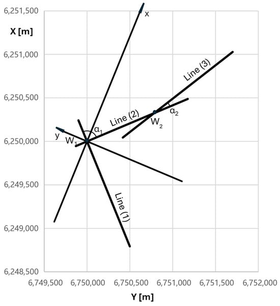
Figure 1. The layout of the main directions of the route in the PL-2000 system.

In the analytical method of designing track geometric systems [32], basic computational operations are performed in the local coordinate system x, y. This system is defined by two intersecting main directions, arranged symmetrically; their intersection point is the origin of the system in question. In the case of modeling reverse curves, it was decided to maintain this principle, determining the local coordinate system (LCS) based on the location of Line 1 and Line 2. This is illustrated in Figure 1 by showing the position of the LCS axes in the PL-2000 system.

The equation of Line 1 in the PL-2000 system is as follows:

$$X=X_{W1}+\tan {\mathit{\Phi }}_1\left(Y-Y_{W1}\right)$$

(1)

and the equation of Line 2 has the form:

$$X=X_{W1}+\tan {\mathit{\Phi }}_2\left(Y-Y_{W1}\right),$$

(2)

where Y_W1 and X_W1 are the coordinates of point W₁, and Φ₁ and Φ₂ are the inclination angles of Line 1 and Line 2, respectively.

When adopting the appropriate numerical values in the calculation example, we were guided by the desire to obtain the greatest possible clarity of the geometric system in the LCS. Therefore, in this case, the coordinates of the main point Y_W1 = 6,750,000 m, X_W1 = 6,250,000 m, and the slope of Line 1 equal to Φ₁ = −3π/8 rad were assumed. The assumed angle of return of the route α₁ = π/2 rad results in the slope of Line 2 equal to Φ₂ = Φ₁ + α₁ = π/8 rad. The above data give the required values of the shifts Y_W1 and X_W1 and the rotation angle β = Φ₂ + α₁/2 = 3π/8 rad, leading to the transformation of coordinates from the PL-2000 system to the local coordinate system. This is performed using the following formulas [34]:

$$x=\left(Y-Y_{W1}\right)\cos \beta -\left(X-X_{{\displaystyle \mathsf{\partial }}W1}\right)\sin \beta ,$$

(3)

$$y=\left(Y-Y_{W1}\right)\sin \beta +\left(X-X_{\mathsf{\partial }W1}\right)\cos \beta .$$

(4)

The angle of inclination of the x-axis in the PL-2000 system is Φ_x = β = 3π/8 rad, so its equation is as follows:

$$X=X_{W1}+\tan {\mathit{\Phi }}_x\left(Y-Y_{W1}\right).$$

(5)

The angle of inclination of the y-axis in this system is equal to Φ_y = β − π/2 = −π/8 rad; hence, the equation of this axis is

$$X=X_{W1}+\tan {\mathit{\Phi }}_y\left(Y-Y_{W1}\right).$$

(6)

Since the assumed angle of the route at point W₂ is equal to α₂ = π/12 rad, the slope of Line 3 is Φ₃ = Φ₂ + α₂ = π/6 rad. From the point of view of operations carried out in the LCS, it turned out to be advantageous to adopt the coordinates of the next principal point: Y_W2 = 6,750,783.938 m and X_W2 = 6,250,324.718 m. The given data result in the equation of Line 3:

$$X=X_{W2}+\tan {\mathit{\Phi }}_3\left(Y-Y_{W2}\right).$$

(7)

3. Local Coordinate System

It should be noted from the outset that the alignment of the main directions of the route in the PL-2000 coordinate system can vary greatly. However, after transformation to the local coordinate system, there are only two possible positions for the designed geometric system: under the x-axis, with negative ordinates and the convexity of the curvilinear elements directed upwards, and above the x-axis, with positive ordinates and the convexity of the curvilinear elements directed downwards [32]. Therefore, strictly speaking, both possible cases should be taken into account when determining the appropriate computational algorithms.

The main directions in Figure 1 indicate that in the LCS, the geometric system under consideration lies below vertex W₁ and its ordinates are negative. This is the case that will be the subject of this article. The resulting formulas can also be applied to the system positioned above the x-axis, after making minor adjustments to the plus and minus signs.

The transfer of the route’s main directions in Figure 1 to the local coordinate system is performed using Equations (3) and (4). This creates the situation shown in Figure 2.

Figure 2. The system of main directions of the route in the local coordinate system.

The origin of the local coordinate system, in which further detailed considerations will be conducted, is located at point W₁(0,0), where Line 1 and Line 2 intersect. This is characteristic of the LCS used in the analytical method of designing geometric systems of the track [32].

The equations of the intersecting lines result from the angle of the route α1 for the first circular arc (marked as Arc I) and are as follows:

$$\begin{array}{c}•\mathrm{for} \mathit{Line} 1:y=s_1\cdot x,s_1=\tan {\phi }_1=\tan {\displaystyle \frac{{\mathsf{\alpha }}_1}{2}},\\ •\mathrm{for} \mathit{Line} 2:y=s_2\cdot x,s_2=\tan {\phi }_2=-\tan {\displaystyle \frac{{\mathsf{\alpha }}_1}{2}},\end{array}$$

where φ₁ and φ₂ are the inclination angles of Line 1 and Line 2 in the LCS. In the given case, the assumed turning angle is α₁ = π/2 rad.

The second circular arc (marked as Arc II) is directed opposite to the preceding arc and connects Line 2 with Line 3. Both lines intersect at point W₂, the coordinates of which, x_W2 and y_W2, result from the coordinates Y_W2 and X_W2. The equation of Line 3 results from the return angle α₂ for the second circular arc:

$$•y=y_{W2}+s_3\left(x-x_{W2}\right),s_3=\tan {\phi }_3=\tan \left(-{\displaystyle \frac{{\mathsf{\alpha }}_1}{2}}+{\mathsf{\alpha }}_2\right).$$

where φ₃ is the angle of inclination of Line 3 in the LCS. In the case under consideration, the coordinates of point W₂ are x_W2 = 600 m, y_W2 = −600 m, and the angle of inclination of the line is equal to φ₃ = −π/6 rad.

As can be seen, the numerical parameters of the considered system of the main directions of the route in the LCS allow for convenient tracking of the design procedure, including, among others, defining individual geometric elements. After completing this procedure, the obtained solution is transferred to the PL-2000 system using transformation formulas [34]:

$$Y=Y_{\mathit{W}1}+x\cdot \cos \beta -y\cdot \sin \beta .$$

(8)

$$X=X_{\mathit{W}1}+x\cdot \sin \beta +y\cdot \cos \beta .$$

(9)

4. Reverse Arcs Radii

The values of the radii of the reverse arcs must correspond to the existing system of main directions. The key issue here is to choose the correct point of connection of both arcs. This point (marked C in Figure 3) is located on Line 2, and the condition $x_C\in \left(x_{W1},x_{W2}\right)$ holds. For the assumed x_C, we determine y_C using the formula

$$y_C=-\left(\tan {\displaystyle \frac{{\mathsf{\alpha }}_1}{2}}\right)x_C.$$

(10)

Then we calculate the distances $\overline{W_{1}C}$ and $\overline{C{W}_2}$.

$$\overline{W_{1}C}=\sqrt{{\left(x_C-x_{W1}\right)}^2+{\left(y_C-y_{W1}\right)}^2},$$

(11)

$$\overline{C{W}_2}=\sqrt{{\left(x_{W2}-x_C\right)}^2+{\left(y_{W2}-y_C\right)}^2}.$$

(12)

Of course, the condition must be met

$$\overline{W_{1}C}+\overline{C{W}_2}=\overline{W_1{W}_2}=\sqrt{{\left(x_{W2}-x_{W1}\right)}^2+{\left(y_{W2}-y_{W1}\right)}^2}.$$

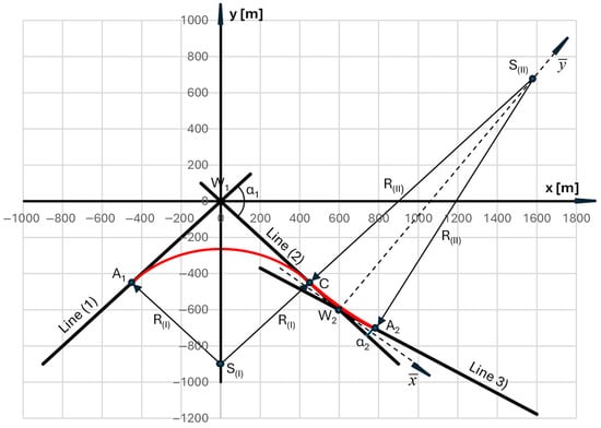
Figure 3. The primary geometric arrangement of reverse arcs in the local coordinate system.

We treat $\overline{W_{1}C}$ and $\overline{C{W}_2}$ as tangents of the corresponding reverse circular arcs. First, we determine the radius R_(I) of Arc I. Since its angle of return is ${\mathsf{\alpha }}_1=\left|{\phi }_2-{\phi }_1\right|$, for φ₁ = π/4 rad, φ₂ = −π/4 rad, we obtain α₁ = π/2 rad. From the formula for the value of the tangent

$$t_1=\overline{W_{1}C}=\left(\tan {\displaystyle \frac{\left|{\phi }_2-{\phi }_1\right|}{2}}\right)R_{(I)}$$

(13)

It follows that

$$R_{(I)}={\displaystyle \frac{t_1}{\tan \frac{\left|{\phi }_2-{\phi }_1\right|}{2}}}.$$

(14)

The return angle of Arc II, with radius R_(II), is ${\mathsf{\alpha }}_2=\left|{\phi }_3-{\phi }_2\right|$. Since in the case under consideration φ₂ = −π/4 rad, φ₃ = −π/6 rad, we obtain α₂ = π/12 rad. The formula for the value of the tangent is

$$t_2=\overline{C{W}_2}=\left(\tan {\displaystyle \frac{\left|{\phi }_3-{\phi }_2\right|}{2}}\right)R_{(II)},$$

(15)

hence

$$R_{(II)}={\displaystyle \frac{t_2}{\tan \frac{\left|{\phi }_3-{\phi }_2\right|}{2}}}.$$

(16)

Table 1 presents the values of the radii of the reverse arcs determined for different coordinates of point C in the considered calculation example.

Table 1. Example values of radii R_(I) and R_(II) for different coordinates of point C.

Abscissa xC [m]	Ordinate yC [m]	Tangent t1 [m]	Radius R(I) [m]	Tangent t2 [m]	Radius R(II) [m]
350	−350	494.075	494.975	353.553	2685.505
375	−375	530.330	530.330	318.198	2416.954
400	−400	565.685	565.685	282.843	2348.404
425	−425	601.041	601.041	247.487	1879.853
450 1	−450 1	636.396 1	636.396 1	212.132 1	1611.303 1
475	−475	671.751	671.751	176.777	1342.752
500	−500	707.107	707.107	141.421	1074.202

¹ Numerical value for the selected case.

As can be seen, for a given arrangement of the main directions of the route and the assumed location of the circular arc connection, there is a specific relationship between the values of these arc radii. Therefore, reverse arcs cannot be shaped arbitrarily; various conditions must be taken into account. Based on the data from Table 1, the case x_C = 450 m, y_C = −450 m was qualified for further analysis. The driving force behind this decision was the desire to achieve a relatively favorable arc radius R_(I) (i.e., one that allows for the highest possible speed), without excessively restricting the area occupied by Arc II. Of course, this decision is purely arbitrary, but Table 1 clearly shows that as R_(I) increases, the value of t₂ decreases. As a result, it was necessary to consider the initial values of the circular arc radii R_(I) = 636.396 m and R_(II) = 1611.303 m.

Entering the designated arcs into the system of main directions allows us to create the original geometric system of reverse arcs. This requires first determining the coordinates of the starting point A₁ for the arc with radius R_(I) and the ending point A₂ for the arc with radius R_(II) (Figure 3). The coordinates of the point where both arcs join (i.e., point C) are already known.

The following formulas apply:

$$x_{A1}=x_{W1}-{\displaystyle \frac{1}{\sqrt{1+s_1^2}}}{t}_1,$$

(17)

$$y_{A1}=y_{W1}-{\displaystyle \frac{s_1}{\sqrt{1+s_1^2}}}{t}_1,$$

(18)

$$x_{A2}=x_{W2}+{\displaystyle \frac{1}{\sqrt{1+s_3^2}}}{t}_2,$$

(19)

$$y_{A2}=y_{W2}+{\displaystyle \frac{s_3}{\sqrt{1+s_3^2}}}{t}_2.$$

(20)

In the case shown in Figure 3, the determined coordinates are as follows: x_A1 = −450 m, y_A1 = −450 m, x_A2 = 783.712 m and y_A2 = −706.066 m.

In the next step, the coordinates of the centers of both circular arcs are determined. For Arc I, lines perpendicular to the corresponding main directions are drawn from points A₁ and C. The center of the arc S_(I) lies at the intersection of these lines. After solving the appropriate system of equations, the formulas for its coordinates are obtained:

$$x_{S(I)}={\displaystyle \frac{s_1{s}_2}{s_2-s_1}}\left({\displaystyle \frac{1}{s_1}}{x}_{A1}-{\displaystyle \frac{1}{s_2}}{x}_C+y_{A1}-y_C\right),$$

(21)

$$y_{S(I)}=y_{A1}-{\displaystyle \frac{1}{s_1}}\left(x_{S(I)}-x_{A1}\right),$$

(22)

The equation of Arc I is as follows:

$$y=y_{S(I)}\pm \sqrt{R_{(I)}^2-{\left(x-x_{S(I)}\right)}^2}.$$

(23)

In the case under consideration, x_S(I) = 0, y_S(I) = −900 m, and the arc equation has the form

$$y=-900+\sqrt{{\left(636.396\right)}^2-x^2}, x\in ⟨-450;450⟩\mathrm{m}.$$

The procedure for Arc II is analogous. Lines perpendicular to the corresponding main directions are drawn from points C and A₂. After solving the appropriate system of equations, the formulas for the coordinates of the center of the arc S_(II) are obtained:

$$x_{S(II)}={\displaystyle \frac{s_2{s}_3}{s_3-s_2}}\left({\displaystyle \frac{1}{s_2}}{x}_C-{\displaystyle \frac{1}{s_3}}{x}_{A2}+y_C-y_{A2}\right),$$

(24)

$$y_{S(II)}=y_{A2}-{\displaystyle \frac{1}{s_3}}\left(x_{S(II)}-x_{A2}\right),$$

(25)

The equation of Arc II has the following form:

$$y=y_{S(II)}\pm \sqrt{R_{(II)}^2-{\left(x-x_{S(II)}\right)}^2}.$$

(26)

In the case under consideration x_S(II) = 1589.363 m, y_S(II) = 689.363 m, and the arc equation is as follows:

$$y=689.363-\sqrt{{\left(1611.303\right)}^2-{\left(x-1589.363\right)}^2}, x\in ⟨450;783.712⟩\mathrm{m}.$$

The inserted reverse arcs are marked in red in Figure 3. The $\overline{x},\overline{y}$ auxiliary coordinate system is also shown there, which will be used to analyze the application of transition curves for Arc II (in Section 7).

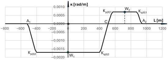
5. Curvature of the Primary Reverse Arc System

The arrangement of primary reverse curves shown in Figure 3 raises serious concerns. These arise from the occurrence of very unfavorable lateral accelerations when the rail vehicle is traveling at a given speed V. This is best seen in the curvature diagram of the geometric system, from which these accelerations directly result.

To determine the curvature graph along the length of the geometric system, a rail vehicle model was used in the form of its rigid base with a length of l_b = 20 m. The curvature value is obtained by tracking the position of the moving center of the rigid base. Of course, this is a very simplified model. In analyzing the mechanical system of a rail vehicle and track, it would be necessary to consider the vehicle’s dynamic characteristics (such as the suspension system and the geometry of the wheel–rail contact). However, in the situation under consideration, this was not necessary. The kinematic parameters used in the design of track geometry assume linear changes over time (and therefore also over length). This applies to both the acceleration rate and the lifting speed of the rolling stock wheel on the gradient due to cant. Figure 4 shows the curvature graph obtained for the system of reverse arcs from Figure 3.

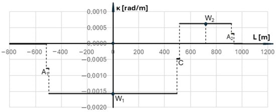
Figure 4. Curvature diagram over the length of the primary reverse arc system.

As can be seen in the graph, there are sudden, abrupt changes in curvature around points A₁, C, and A₂. This causes two impacts at each point, transverse to the track, which can be easily observed, for example, on tram lines. However, travel on these lines in areas of abrupt changes in curvature is usually very slow. On railway lines, much higher speeds apply, meaning travel times are shorter, and therefore, the impact-mitigating effect of the rigid base is limited. Therefore, from a theoretical perspective, travel on the discussed geometric configuration could be achieved at low speeds.

Because in the real track, due to its stiffness, the curvature at the joints of individual geometric elements is smoothed out, certain simplifying assumptions can be made to estimate the possible train speed. This involves the assumption (which is highly debatable, by the way) that the change in curvature at critical points occurs not abruptly, but linearly along the length of the rigid base.

The velocity on the geometric system of reverse curves results from the situation occurring at point C, i.e., at the point of contact of Arc I and Arc II. These are curves without cant (i.e., h₁ = 0 and h₂ = 0). The values of unbalanced acceleration, directed in opposite directions, are as follows:

$$a_{m1}={\displaystyle \frac{V^2}{{\left(3.6\right)}^2{R}_{(I)}}}, a_{m2}={\displaystyle \frac{V^2}{{\left(3.6\right)}^2{R}_{(II)}}},$$

where the velocity V is expressed in km/h, the radii R_(I) and R_(II) in meters, and the accelerations a_m1 and a_m2 in m/s².

According to Polish regulations [35], acceleration values should be less than a_per = 0.85 m/s², but this condition is insufficient. The acceleration increase condition should also be checked:

$$\psi ={\displaystyle \frac{\left(a_{m1}+a_{m2}\right)\cdot V}{3.6\cdot l_b}}\le {\psi }_{per}$$

for the assumed length of the rigid wagon base, where ψ is expressed in m/s³. The acceleration increase should be smaller than ψ_per = 0.5 m/s³ [36]. The relevant analysis is presented in Table 2.

Table 2. Determining the approximate train speed for the original reverse curves system.

Train Speed V [km/h]	Radius R(I) [m]	Acceleration am1 [m/s2]	Radius R(II) [m]	Acceleration am2 [m/s2]	Sum of Accelerations am1 + am2 [m/s2]	Acceleration Increase ψ [m/s3]
50	636.396	0.303115	1611.303	0.119718	0.422833	0.293634
55	636.396	0.366769	1611.303	0.144858	0.511627	0.390827
60	636.396	0.436486	1611.303	0.172393	0.608879	0.507399
65	636.396	0.512264	1611.303	0.202323	0.714587	0.645113
70	636.396	0.594105	1611.303	0.234646	0.828752	0.805731

In the case under consideration, this gives a speed of V_max = 60 km/h for which ψ = 0.507399 m/s³, i.e. it is lower than the permissible value. This speed is relatively low and, moreover, not entirely reliable. Therefore, modeling of reverse curves should be continued by introducing transition curves for both existing circular arcs. This is possible if there is an appropriate distance between vertices W₁ and W₂ (it cannot be too small).

The transition curves are entered separately for Arc I and Arc II. As a result of this operation, the radii of these arcs are reduced. The corresponding calculation procedure for Arc I is performed in the local coordinate system, while for Arc II in the $\overline{x},\overline{y}$ auxiliary coordinate system, with subsequent transfer of the obtained solution to the LCS.

The decision was made to use transition curves in the form of a clothoid, written as parametric equations x(l) and y(l). It was recognized that the analytical design method should not utilize simplified solutions, which undoubtedly include the third-degree parabola (also known as the cubic parabola). When determining the equation of this curve, it is assumed that the modeled curvature κ(l) refers to its projection onto the x-axis (i.e., that l = x), and creates an incorrect formula $y^{″}(x)=\kappa (x)$; after double integration, the equation of the curve is obtained in the form of an explicit function y(x). The third-degree parabola is still commonly used on railways, but with current computational capabilities, it no longer has any practical justification.

6. Applying Transition Curves for the First Circular Arc

For Arc I, with the primary (initial) radius R_(I), transition curves of different lengths L_(I)i, i = 1, 2, … can be used. Figure 5 shows a fragment of the local coordinate system containing the effects of using symmetric transition curves of length 50 m and 100 m. It should be noted here that no detailed analysis was planned regarding the selection of transition curve lengths. In the case of reverse curves, train speeds were determined not by the lengths of transition curves (which could be easily corrected), but by the value of the smaller radius of the circular arc. The initial geometric system is marked in red; the system with curves of length L_(I)1 = 50 m is marked in green; and the system with curves of length L_(I)2 = 100 m is marked in purple.

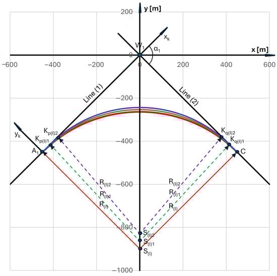
Figure 5. Effects of using symmetrical transition curves of 50 m and 100 m length for Arc I (in the local coordinate system).

The given task is to introduce transition curves p and q in the form of a clothoid with an assumed, differentiated length L_(I)i at both ends of Arc I (i.e., originating from points A₁ and C). Since the designed geometric system is symmetrical, it is sufficient to consider one (in this case, the left) half of it (i.e., with transition curve p) in detail. The straight segment on the left side of the system (i.e., Line 1) is the abscissa axis of the Cartesian coordinate system x_k, y_k, associated with the given transition curve. The origin of this system is at point A₁. We are interested in the coordinates of the curve’s endpoint (i.e., point K_p(I)i) in this system; they result from the corresponding parametric equations x_k(l) and y_k(l) for l = L_(I)i. Since—as it turns out—we must take into account the need to correct the radius of the circular arc, the transition curve equations must use different values of the arc radius R_(I)i. When using a transition curve in the form of a clothoid, the following parametric equations apply in the x_k, y_k system:

$$x_k(L_{(I)i})=L_{(I)i}-{\displaystyle \frac{L_{(I)i}^3}{40\cdot R_{(I)i}^2}}+{\displaystyle \frac{L_{(I)i}^5}{3456\cdot R_{(I)i}^4}},$$

(27)

$$y_k(L_{(I)i})=-{\displaystyle \frac{L_{(I)i}^2}{6\cdot R_{(I)i}}}+{\displaystyle \frac{L_{(I)i}^4}{336\cdot R_{(I)i}^3}}-{\displaystyle \frac{L_{(I)i}^6}{\mathrm{42,240}\cdot R_{(I)i}^5}}$$

(28)

while the angle of inclination ${\mathrm{\Theta }}_k(L_{(I)i})$ at the end of the curve is determined from the relationship

$${\mathrm{\Theta }}_k(L_{(I)i})=-{\displaystyle \frac{L_{(I)i}}{2\cdot R_{(I)i}}}.$$

(29)

The transformation of the transition curve to the x, y coordinate system is performed by rotating the reference system by an angle of α₁/2 and shifting the curve origin to point A₁. The corresponding formulas depend on the direction of rotation. This operation yields the desired values of the transition curve projections onto the horizontal and vertical axes, which are the coordinates of the curve’s endpoint. If the x_k, y_k system is rotated clockwise (as in Figure 5), the following relations are obtained:

$$x_{Kp(I)i}=x(L_{(I)i})=x_{A1}+x_k(L_{(I)i})\cdot \cos {\displaystyle \frac{{\mathsf{\alpha }}_1}{2}}-y_k(L_{(I)i})\cdot \sin {\displaystyle \frac{{\mathsf{\alpha }}_1}{2}},$$

(30)

$$y_{Kp(I)i}=y(L_{(I)i})=y_{A1}+x_k(L_{(I)i})\cdot \sin {\displaystyle \frac{{\mathsf{\alpha }}_1}{2}}+y_k(L_{(I)i})\cdot \cos {\displaystyle \frac{{\mathsf{\alpha }}_1}{2}}.$$

(31)

The angle of inclination Θ(L_(I)i) at the end of the curve is determined from the formula

$${\mathrm{\Theta }}_{Kp(I)i}=\mathrm{\Theta }(L_{(I)i})=-{\displaystyle \frac{L_{(I)i}}{2\cdot R_{(I)i}}}+{\displaystyle \frac{{\mathsf{\alpha }}_1}{2}}.$$

(32)

Since the introduction of this transition curve is performed while maintaining the position of its starting point (i.e., point A₁), it is necessary to correct the position of the circular arc so that it starts at the point with coordinates x_Kp(I)i and y_Kp(I)i, the angle of inclination of the tangent is Θ_Kp(I)i and the condition of symmetry of the entire system is met (i.e., Θ(0) = 0). This is illustrated in the situation shown in Figure 5.

In this situation, the condition Θ(0) = 0 requires a correction of the arc radius value. This is directly related to the assumed transition curve length. The final solution to the problem is achieved for a specific value of L_(I)i, which is considered the most favorable.

Determining the corrected radius R_(I)i requires determining the coordinates of the center S_(I)i of the corresponding circular arc. It lies on the line perpendicular to the tangent at the end of the transition curve, with the equation

$$y(x)=y_{Kp(I)i}-{\displaystyle \frac{1}{\tan {\mathrm{\Theta }}_{Kp(I)i}}}\left(x-x_{Kp(I)i}\right),$$

at a distance R_(I)i from the point K_p(I)i; it follows from this

$$\sqrt{{\left(x_{S(I)i}-x_{Kp(I)i}\right)}^2+{\left(y_{S(I)i}-y_{Kp(I)i}\right)}^2}=R_{(I)i}.$$

By solving the appropriate system of equations, we obtain the desired coordinates

$$x_{S(I)i}=x_{Kp(I)i}+{\displaystyle \frac{\tan {\mathrm{\Theta }}_{Kp(I)i}}{\sqrt{1+{\left(\tan {\mathrm{\Theta }}_{Kp(I)i}\right)}^2}}}{R}_{(I)i},$$

(33)

$$y_{S(I)i}=y_{Kp(I)i}-{\displaystyle \frac{1}{\sqrt{1+{\left(\tan {\mathrm{\Theta }}_{Kp(I)i}\right)}^2}}}{R}_{(I)i}.$$

(34)

The necessity of fulfilling the condition x_S(I)i = 0 means that

$$R_{(I)i}=-{\displaystyle \frac{\sqrt{1+{\left(\tan {\mathrm{\Theta }}_{Kp(I)i}\right)}^2}}{\tan {\mathrm{\Theta }}_{Kp(I)i}}}{x}_{Kp(I)i},$$

(35)

determining the coordinates of point S_(I)i with a changing value of this radius.

Direct determination of the corrected arc radius R_(I)i using Equation (35) is obviously impossible, because both x_Kp(I)i and Θ_Kp(I)i depend on the value of R_(I)i. What remains is the iterative way, i.e., substituting changing values of R_(I)i until the key condition x_S(I)i = 0 is met. There was no need to specify the number of iterations, computation time or convergence speed; the end of the calculations was determined by the practical accuracy of determining the radius value, which was 1 mm. The final part of the calculations for the selected case (with α₁ = π/2 rad, x_A1 = −450 m, y_A1 = −450 m and L_(I)1 = 50 m) is shown in Table 3.

Table 3. Determining the corrected radius of the first arc for L_(I)1 = 50 m.

Radius R(I)1 [m]	Abscissa xk(L(I)1) [m]	Ordinate yk(L(I)1) [m]	Angle Θk(L(I)1) [rad]	Abscissa xKp(I)1 [m]	Ordinate yKp(I)1 [m]	Angle ΘKp(I)1 [rad]	Abscissa xS(I)1 [m]	Ordinate yS(I)1 [m]
611.230	49.99164	−0.68160	0.0409	−414.169	−415.133	0.744497	0.002060594	−864.649
611.229	49.99164	−0.68161	0.0409	−414.169	−415.133	0.744497	0.001353681	−864.648
611.228	49.99164	−0.68161	0.0409	−414.169	−415.133	0.744497	0.000646768	−864.647
611.227 1	49.99164	−0.68161	0.0409	−414.169	−415.133	0.744497	−0.00006014	−864.647 1
611.226	49.99164	−0.68161	0.0409	−414.169	−415.133	0.744497	−0.00076706	−864.646
611.225	49.99164	−0.68161	0.0409	−414.169	−415.133	0.744497	−0.00147397	−864.645
611.224	49.99164	−0.68161	0.0409	−414.169	−415.133	0.744497	−0.00218088	−864.644
611.223	49.99164	−0.68161	0.0409	−414.169	−415.133	0.744497	−0.00288780	−864.644
611.222	49.99164	−0.68161	0.0409	−414.169	−415.133	0.744496	−0.00359471	−864.643

¹ Determined value of the radius of Arc I.

Taking into account the appropriate number of decimal places for the determined abscissa, x_S(I)1 indicated the corrected circular arc radius R_(I)1 = 611.227 m (marked in bold in Table 3). Thus, the circular arc of radius R_(I), which is part of the reverse arc, is replaced by a circular arc of radius R_(I)1 and two transition curves of length L_(I)1 = 50 m (Figure 5).

The general equation of a circular arc with radius R_(I)i has the form

$$y=y_{S(I)i}+\sqrt{R_{(i)i}^2-x^2}, x\in ⟨x_{Kp(I)i},x_{Kq(I)i}⟩.$$

(36)

Taking into account the existing symmetry, the entire arrangement of the first arc is described as follows:

• for $x\in ⟨x_{A1},x_{Kp(I)i}⟩$, that is $l\in ⟨0,L_{(I)i}⟩$

$$\begin{gathered} x(l)=x_{A1}+x_k(l)\cdot \cos {\displaystyle \frac{{\mathsf{\alpha }}_1}{2}}-y_k(l)\cdot \sin {\displaystyle \frac{{\mathsf{\alpha }}_1}{2}}, \\ y(l)=y_{A1}+x_k(l)\cdot \sin {\displaystyle \frac{{\mathsf{\alpha }}_1}{2}}+y_k(l)\cdot \cos {\displaystyle \frac{{\mathsf{\alpha }}_1}{2}}, \end{gathered}$$

where

$$\begin{gathered} x_k(l)=l-{\displaystyle \frac{l^5}{40\cdot R_{(I)i}^2\cdot L_{(I)i}^2}}+{\displaystyle \frac{l^9}{3456\cdot R_{(I)i}^4\cdot L_{(I)i}^4}}, \\ {y}_k(l)=-{\displaystyle \frac{l^3}{6\cdot R_{(I)i}\cdot l_{(I)i}}}+{\displaystyle \frac{l^7}{336\cdot R_{(I)i}^3\cdot L_{(I)i}^3}}-{\displaystyle \frac{l^{11}}{\mathrm{42,240}\cdot R_{(I)i}^5\cdot L_{(I)i}^5}}. \end{gathered}$$

• for $x\in ⟨x_{Kp(I)i},x_{Kq(I)i}⟩$, where x_Kq(I)i = −x_Kp(I)i

$$y=y_{S(I)i}+\sqrt{R_{(I)i}^2-x^2}.$$

• for $x\in ⟨x_{Kq(I)i},x_C⟩$, that is $l\in ⟨-L_{(I)i},0⟩$

$$\begin{gathered} x(l)=x_C+x_k(l)\cdot \cos {\displaystyle \frac{{\mathsf{\alpha }}_1}{2}}+y_k(l)\cdot \sin {\displaystyle \frac{{\mathsf{\alpha }}_1}{2}}, \\ y(l)=y_C-x_k(l)\cdot \sin {\displaystyle \frac{{\mathsf{\alpha }}_1}{2}}+y_k(l)\cdot \cos {\displaystyle \frac{{\mathsf{\alpha }}_1}{2}}. \end{gathered}$$

where

$$\begin{gathered} x_k(l)=l-{\displaystyle \frac{l^5}{40\cdot R_{(I)i}^2\cdot L_{(I)i}^2}}+{\displaystyle \frac{l^9}{3456\cdot R_{(I)i}^4\cdot L_{(I)i}^4}}, \\ {y}_k(l)={\displaystyle \frac{l^3}{6\cdot R_{(I)i}\cdot L_{(I)i}}}-{\displaystyle \frac{l^7}{336\cdot R_{(I)i}^3\cdot L_{(I)i}^3}}+{\displaystyle \frac{l^{11}}{\mathrm{42,240}\cdot R_{(I)i}^5\cdot L_{(I)i}^5}}. \end{gathered}$$

In the situation shown in Figure 5, L_(I)1 = 50 m was first assumed. Since α₁ = π/2 rad, x_A1 = −450 m and y_A1 = −450 m, the coordinates of the end of the first transition curve in the x_k, y_k system are as follows: x_k(L_(I)1) = 49.992 m, y_k(L_(I)1) = −0.665 m. The angle of inclination of the tangent is Θ(L_(I)1) = −0.03928 rad. The coordinates of the center of the corrected arc are: x_S(I)1 = 0, y_S(I)1 = −864.647 m. This corresponds to the following values in the local coordinate system: x_Kp(I)1 = −414.187 m, y_Kp(I)1 = −415.113 m, Θ_Kp(I)1 = 0.746114 rad, x(0) = 0, y(0) = −253.420 m, x_Kq(I)1 = 414.187 m, y_Kq(I)1 = −415.113 m, Θ_Kq(I)1 = −0.746114 rad, x_C = 450 m and y_C = −450 m. The entire geometric system is shown in Figure 5 (the circular arc is marked in green).

The next step was to assume the length L_(I)2 = 100 m (while maintaining α₁ = π/2 rad, x_A1 = −450 m, and y_A1 = −450 m). As before, the radius R_(I)2 should be determined numerically by specifying the coordinates of point S_(I)2 with varying values of this radius. The basic criterion for solving the problem is to meet the key condition x_S(I)2 = 0. The final part of the calculations for the discussed case is shown in Table 4.

Table 4. Determining the corrected radius of the first curve for L_(I)2 = 100 m.

Radius R(I)2 [m]	Abscissa xk(L(I)2) [m]	Ordinate yk(L(I)2) [m]	Angle Θk(L(I)2) [rad]	Abscissa xKp(I)2 [m]	Ordinate yKp(I)2 [m]	Angle ΘKp(I)2 [rad]	Abscissa xS(I)2 [m]	Ordinate yS(I)2 [m]
585.694	99.92715	−2.84415	−0.08537	−377.330	−381.352	0.700029	−0.00213926	−829.304
585.695	99.92715	−2.84414	−0.08537	−377.330	−381.352	0.700029	−0.00143299	−829.305
585.696	99.92715	−2.84414	−0.08537	−377.330	−381.352	0.700030	−0.00072671	−829.306
585.697 1	99.92715	−2.84413	−0.08537	−377.330	−381.352	0.700030	−0.00002043	−829.306
585.698	99.92715	−2.84413	−0.08537	−377.330	−381.352	0.700030	0.00068585	−829.307
585.699	99.92715	−2.84412	−0.08537	−377.330	−381.352	0.700030	0.00139212	−829.308
585.700	99.92715	−2.84412	−0.08537	−377.330	−381.352	0.700030	0.00209840	−829.309

¹ Determined value of the radius of Arc I.

Taking into account the appropriate number of decimal places for the determined abscissa x_S(I)2 indicates a corrected circular arc radius R_(I)2 = 585.697 m. Thus, the circular arc of radius R_(I), which is part of the reverse arc, is replaced by a circular arc of the given radius and two transition curves of 100 m length. This is shown in Figure 5, where the circular arc is marked in purple.

The coordinates of the end of the first transition curve in the x_k, y_k system are as follows: x_k(L_(I)2) = 99.927 m, y_k(L_(I)2) = −2.844 m. The angle of inclination of the tangent is Θ(L_(I)2) = −0.085368 rad. The coordinates of the center of the corrected arc are: x_S(I)2 = 0, y_S(I)2 = −829.306 m. This corresponds to the following values in the local coordinate system: x_Kp(I)2 = −377.330 m, y_Kp(I)2 = −381.352 m, Θ_Kp(I)2 = 0.70003 rad, x(0) = 0, y(0) = −243.609 m, x_Kq(I)2 = 377.330 m, y_Kq(I)2 = −381.352 m, Θ_Kq(I)2 = −0.70003 rad, x_C = 450 m and y_C = −450 m.

7. Applying Transition Curves for the Second Circular Arc

The transition curves at Arc II (with radius R_(II)) are inserted in the $\overline{x},\overline{y}$ auxiliary coordinate system (Figure 3). This system has its origin at point W₂, and the ordinate axis on the line passing through points W₂ and S_(II). The equation of the axes in the LCS is as follows:

$$y=y_{W2}+{\displaystyle \frac{y_{S(II)}-y_{W2}}{x_{S(II)}-x_{W2}}}\left(x-x_{W2}\right).$$

(37)

The $\overline{x}$ axis passes through point W₂ perpendicularly to the $\overline{y}$ axis; therefore, it is described by the equation

$$y=y_{W2}-{\displaystyle \frac{x_{S(II)}-x_{W2}}{y_{S(II)}-y_{W2}}}\left(x-x_{W2}\right)$$

(38)

The separated auxiliary coordinate system is shown in Figure 6. It contains the effects of applying symmetrical transition curves in the form of a clothoid for an arc with an initial radius R_(II). The primary geometric system (without transition curves) is marked in red, which, however—in the adopted drawing scale—has been obscured by the system with curves of length L_(II)1 = 50 m, marked in purple.

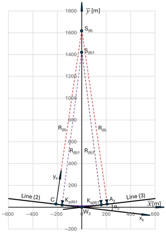
Figure 6. A circular arc with a larger radius (located between points C and A₂), corrected by introducing transition curves (marked in purple).

In the $\overline{x},\overline{y}$ system, the inclinations of the main directions intersecting at point W₂(0,0) result from the angle of inclination α₂. The angle of inclination of Line 2 is −α₂/2, and of Line 3: α₂/2. The abscissa of point S_(II) is equal to zero, and the ordinate results from the relationship:

$${\overline{y}}_{S(II)}=\sqrt{{\left(x_{S(II)}-x_{W2}\right)}^2+{\left(y_{S(II)}-y_{W2}\right)}^2}.$$

(39)

Point C has coordinates:

$${\overline{x}}_C=-R_{(II)}\cos {\displaystyle \frac{{\mathsf{\alpha }}_2}{2}}\tan {\displaystyle \frac{{\mathsf{\alpha }}_2}{2}},$$

(40)

$${\overline{y}}_C=R_{(II)}\sin {\displaystyle \frac{{\mathsf{\alpha }}_2}{2}}\tan {\displaystyle \frac{{\mathsf{\alpha }}_2}{2}},$$

(41)

and point A₂:

$${\overline{x}}_{A2}=R_{(II)}\cos {\displaystyle \frac{{\mathsf{\alpha }}_2}{2}}\tan {\displaystyle \frac{{\mathsf{\alpha }}_2}{2}},$$

(42)

$${\overline{y}}_{A2}=R_{(II)}\sin {\displaystyle \frac{{\mathsf{\alpha }}_2}{2}}\tan {\displaystyle \frac{{\mathsf{\alpha }}_2}{2}}.$$

(43)

The equation of Line 2 has the form

$$\overline{y}=-\left(\tan {\displaystyle \frac{{\mathsf{\alpha }}_2}{2}}\right)\cdot \overline{x},$$

(44)

and the equation of Line 3

$$\overline{y}=\left(\tan {\displaystyle \frac{{\mathsf{\alpha }}_2}{2}}\right)\cdot \overline{x}.$$

(45)

The radius of the arc starting from point C lies on the line with equation

$$\overline{y}={\overline{y}}_C+{\displaystyle \frac{{\overline{y}}_{S(II)}-{\overline{y}}_C}{{\overline{x}}_{S(II)}-{\overline{x}}_C}}\left(\overline{x}-{\overline{x}}_C\right),$$

(46)

and the radius originating from point A₂ is located on the straight line

$$\overline{y}={\overline{y}}_{A2}+{\displaystyle \frac{{\overline{y}}_{S(II)}-{\overline{y}}_{A2}}{{\overline{x}}_{S(II)}-{\overline{x}}_{A2}}}\left(\overline{x}-{\overline{x}}_{A2}\right).$$

(47)

The equation of Arc II is as follows:

$$\overline{y}={\overline{y}}_{S(II)}+\sqrt{R_{(II)}^2-{\left(\overline{x}-{\overline{x}}_{S(II)}\right)}^2}.$$

(48)

In the example considered, α₂ = π/12 rad. We therefore obtain

$$\begin{array}{cc}{\overline{x}}_{S(II)}=0,& {\overline{y}}_{S(II)} = 1625.206\mathrm{m},\\ {\overline{x}}_C=-210.317 \mathrm{m},& {\overline{y}}_C = 27.689\mathrm{m},\\ {\overline{x}}_{A2}=210.317 \mathrm{m},& {\overline{y}}_{A2} = 27.689\mathrm{m}.\end{array}$$

We introduce transition curves p and q in the form of a clothoid of length L_(II)i, i = 1, 2, … at both ends of Arc II (i.e., starting from points C and A₂). For symmetry reasons, we consider only the left half of the geometric system (with curve p). The segment of Line 2 is the abscissa axis of the Cartesian coordinate system x_k, y_k, associated with the given transition curve. The origin of this system is at point C. We are interested in the coordinates of the endpoint of the curve in this system (i.e., point K_p(II)i). As in Section 6, in the equations of the transition curve, we must operate with different values of R_(II)i of the arc radius. When using a transition curve in the form of a clothoid, Equation (27) applies to x_k(L_(II)i), and Equation (49) applies to y_k(L_(II)i)

$$y_k(L_{(II)i})={\displaystyle \frac{L_{(II)i}^2}{6\cdot R_{(II)i}}}-{\displaystyle \frac{L_{(II)i}^4}{336\cdot R_{(II)i}^3}}+{\displaystyle \frac{L_{(II)i}^6}{\mathrm{42,240}\cdot R_{(II)i}^5}},$$

(49)

while the angle of inclination Θ_k(L_(II)i) at the end of the curve is determined from the dependence

$${\mathrm{\Theta }}_k(L_{(II)i})={\displaystyle \frac{L_{(II)i}}{2\cdot R_{(II)i}}}.$$

(50)

The transformation of the transition curve into the $\overline{x},\overline{y}$ coordinate system is performed by rotating the reference system by an angle α₂/2 and shifting the curve origin to point C. The corresponding formulas depend on the direction of rotation. This operation results in the desired values of the projections of the transition curve onto the horizontal and vertical axes, which are the coordinates of the end K_p(II)i of the curve. If the x_k, y_k system is rotated to the left (as in Figure 6), the following values are obtained:

$${\overline{x}}_{Kp(II)i}=\overline{x}(L_{(II)i})={\overline{x}}_C+x_k(L_{(II)i})\cdot \cos {\displaystyle \frac{{\mathsf{\alpha }}_2}{2}}+y_k(L_{(II)i})\cdot \sin {\displaystyle \frac{{\mathsf{\alpha }}_2}{2}}.$$

(51)

$${\overline{y}}_{Kp(II)i}=\overline{y}(L_{(II)i})={\overline{y}}_C-x_k(L_{(II)i})\cdot \sin {\displaystyle \frac{{\mathsf{\alpha }}_2}{2}}+y_k(L_{(II)i})\cdot \cos {\displaystyle \frac{{\mathsf{\alpha }}_2}{2}}$$

(52)

The angle of inclination Θ(L_(II)i) at the end of the curve is determined from the relationship

$${\overline{\mathrm{\Theta }}}_{Kp(II)i}=\overline{\mathrm{\Theta }}(L_{(II)i})={\displaystyle \frac{L_{(II)i}}{2\cdot R_{(II)i}}}-{\displaystyle \frac{{\mathsf{\alpha }}_2}{2}}.$$

(53)

Since the introduction of this transition curve is performed while maintaining the position of its starting point (i.e., point C), it is necessary to correct the position of the circular arc so that it starts at the point with coordinates ${\overline{x}}_{Kp(II)i}$ and ${\overline{y}}_{Kp(II)i}$, the angle of inclination of the tangent is there ${\overline{\mathrm{\Theta }}}_{Kp(II)i}$ and the condition of symmetry of the entire system is met (i.e., $\overline{\mathrm{\Theta }}\left(0\right)=0$). This last condition requires the value of the arc radius to be corrected. This is directly related to the assumed length of the transition curve. Determining the corrected radius R_(II)i requires determining the coordinates of the center S_(II)i of the corresponding circular arc. It lies on the line perpendicular to the tangent at the end of the transition curve, with the equation

$$\overline{y}\left(\overline{x}\right)={\overline{y}}_{Ka(II)i}-{\displaystyle \frac{1}{\tan {\stackrel{-}{\mathrm{\Theta }}}_{Ka(II)i}}}\left(\overline{x}-{\overline{x}}_{Ka(II)i}\right).$$

The center of the corrected circular arc lies on this line, at a distance R_(II) from the point K_p(II)i. This gives the system of equations:

$${\overline{y}}_{S(II)i}={\overline{y}}_{Kp(II)i}-{\displaystyle \frac{1}{\tan {\stackrel{-}{\mathrm{\Theta }}}_{Kp(II)i}}}\left({\overline{x}}_{S(II)i}-{\overline{x}}_{Kp(II)i}\right),$$

$$\sqrt{{\left({\overline{x}}_{S(II)i}-{\overline{x}}_{Kp(II)i}\right)}^2+{\left({\overline{y}}_{S(II)i}-{\overline{y}}_{Kp(II)i}\right)}^2}=R_{(II)i}.$$

By solving this system of equations, we obtain the desired coordinates

$${\overline{x}}_{S(II)i}={\overline{x}}_{Kp(II)i}-{\displaystyle \frac{\tan {\stackrel{-}{\mathrm{\Theta }}}_{Kp(II)i}}{\sqrt{1+{\left(\tan {\stackrel{-}{\mathrm{\Theta }}}_{Kp(II)i}\right)}^2}}}{R}_{(II)i},$$

(54)

$${\overline{y}}_{S(II)i}={\overline{y}}_{Kp(II)i}+{\displaystyle \frac{1}{\sqrt{1+{\left(\tan {\stackrel{-}{\mathrm{\Theta }}}_{Kp(II)i}\right)}^2}}}{R}_{(II)i}.$$

(55)

The correct solution requires that the condition ${\overline{x}}_{S(II)i}=0$. This means that

$$R_{(II)i}=-{\displaystyle \frac{\sqrt{1+{\left(\tan {\stackrel{-}{\mathrm{\Theta }}}_{Kp(II)i}\right)}^2}}{\tan {\stackrel{-}{\mathrm{\Theta }}}_{Kp(II)i}}}{\overline{x}}_{Kp(II)i}.$$

(56)

In the above relation, the abscissa ${\overline{x}}_{Kp(II)i}$ is described by Equation (51), in which x_k(L_(II)i) and y_k(L_(II)i) depend on the radius R_(II)i; this also applies to the angle ${\stackrel{-}{\mathrm{\Theta }}}_{Kp(II)i}$.

In this situation, as in Section 6, the radius R_(II)i should be determined iteratively, changing the values of this radius when determining the coordinates of point S_(II)i. The solution to the problem is determined by fulfilling the condition ${\overline{x}}_{S(II)i}=0$. The final fragment of the calculations for the selected case (with α₂ = π/12 rad, x_C = −210.317 m, y_C = 27.689 m and L_(II)i = L_(II)1 = 50 m) is shown in Table 5.

Table 5. Determining the corrected radius of the second arc.

Radius R(II)1 [m]	Abscissa xk(L(II)1) [m]	Ordinate yk(L(II)1) [m]	Angle Θk(L(II)1) [rad]	$\mathbf{Abscissa} {\overline{\mathit{x}}}_{\mathit{K}\mathit{p}(\mathit{I}\mathit{I})\mathit{i}}$ [m]	Ordinate ${\overline{\mathit{y}}}_{\mathit{K}\mathit{p}(\mathit{I}\mathit{I})\mathit{i}}$ [m]	$\mathbf{Angle} {\overline{\mathit{\Theta }}}_{\mathit{K}\mathit{p}(\mathit{I}\mathit{I})\mathit{i}}$ [rad]	$\mathbf{Abscissa} {\overline{\mathit{x}}}_{\mathit{S}(\mathit{I}\mathit{I})1}$ [m]	$\mathbf{Ordinate} {\overline{\mathit{y}}}_{\mathit{S}(\mathit{I}\mathit{I})1}$ [m]
1,421,341	49.99845	0.293144	0.017589	−160,708	21,453	−0.11331	0.000449570	1,433,680
1,421,340	49.99845	0.293144	0.017589	−160,708	21,453	−0.11331	0.000314437	1,433,679
1,421,339	49.99845	0.293144	0.017589	−160,708	21,453	−0.11331	0.000183918	1,433,678
1,421,338 1	49.99845	0.293145	0.017589	−160,708	21,453	−0.11331	0.000053398	1,433,677
1,421,337	49.99845	0.293145	0.017589	−160,708	21,453	−0.11331	−0.00007712	1,433,676
1,421,336	49.99845	0.293145	0.017589	−160,708	21,453	−0.11331	−0.00020764	1,433,675
1,421,335	49.99845	0.293145	0.017589	−160,708	21,453	−0.11331	−0.00033816	1,433,674
1,421,334	49.99845	0.293145	0.017589	−160,708	21,453	−0.11331	−0.00046868	1,433,673
1,421,333	49.99845	0.293145	0.017589	−160,708	21,453	−0.11331	−0.00059920	1,433,672

¹ Determined value of the radius of Arc II.

Taking into account the appropriate number of decimal places for the determined abscissa, x_S(II)i indicated the corrected circular arc radius R_(II)i = R_(II)1 = 1421.338 m. Thus, the circular arc of radius R_(II), which is part of the reverse arc, is replaced by a circular arc of radius R_(II)1 and two transition curves of length L_(II)1 (Figure 6).

The equation of a circular arc with radius R_(II)i in the $\overline{x},\overline{y}$ system has the form

$$\overline{y}={\overline{y}}_{S(II)i}-\sqrt{R_{(II)i}^2-{\overline{x}}^2}, \overline{x}\in ⟨{\overline{x}}_C,{\overline{x}}_{A2}⟩.$$

(57)

The entire system is described as follows:

• for $\overline{x}\in ⟨{\overline{x}}_C,{\overline{x}}_{Kp(II)i}⟩$, that is $l\in ⟨0,L_{(II)i}⟩$

$$\begin{gathered} \overline{x}(l)={\overline{x}}_C+x_k(l)\cdot \cos {\displaystyle \frac{{\mathsf{\alpha }}_2}{2}}+y_k(l)\cdot \sin {\displaystyle \frac{{\mathsf{\alpha }}_2}{2}}, \\ \overline{y}(l)={\overline{y}}_C-x_k(l)\cdot \sin {\displaystyle \frac{{\mathsf{\alpha }}_2}{2}}+y_k(l)\cdot \cos {\displaystyle \frac{{\mathsf{\alpha }}_2}{2}}, \end{gathered}$$

where

$$\begin{gathered} x_k(l)=l-{\displaystyle \frac{l^5}{40\cdot R_{(II)i}^2\cdot L_{(II)i}^2}}+{\displaystyle \frac{l^9}{3456\cdot R_{(II)i}^4\cdot L_{(II)i}^4}}, \\ {y}_k(l)={\displaystyle \frac{l^3}{6\cdot R_{(II)i}\cdot L_{(II)i}}}-{\displaystyle \frac{l^7}{336\cdot R_{(II)i}^3\cdot L_{(II)i}^3}}+{\displaystyle \frac{l^{11}}{\mathrm{42,240}\cdot R_{(II)i}^5\cdot L_{(II)i}^5}} \end{gathered}$$

• for $\overline{x}\in ⟨{\overline{x}}_{Kp(II)i},{\overline{x}}_{Kq(II)i}⟩$, where ${\overline{x}}_{Kq(II)i}=-{\overline{x}}_{Kp(II)i}$

$$\overline{y}={\overline{y}}_{S(II)i}-\sqrt{R_{(II)i}^2-{\overline{x}}^2}$$

• for $\overline{x}\in ⟨{\overline{x}}_{Kq(II)i},{\overline{x}}_{A2}⟩$, that is $l\in ⟨-L_{(II)i},0⟩$

$$\begin{gathered} \overline{x}(l)={\overline{x}}_{A2}+x_k(l)\cdot \cos {\displaystyle \frac{{\mathsf{\alpha }}_2}{2}}-y_k(l)\cdot \sin {\displaystyle \frac{{\mathsf{\alpha }}_2}{2}}, \\ \overline{y}(l)={\overline{y}}_{A2}+x_k(l)\cdot \sin {\displaystyle \frac{{\mathsf{\alpha }}_2}{2}}+y_k(l)\cdot \cos {\displaystyle \frac{{\mathsf{\alpha }}_2}{2}}. \end{gathered}$$

where

$$\begin{gathered} x_k(l)=l-{\displaystyle \frac{l^5}{40\cdot R_{(II)i}^2\cdot L_{(II)i}^2}}+{\displaystyle \frac{l^9}{3456\cdot R_{(II)i}^4\cdot L_{(II)i}^4}}, \\ {y}_k(l)=-{\displaystyle \frac{l^3}{6\cdot R_{(II)i}\cdot L_{(II)i}}}+{\displaystyle \frac{l^7}{336\cdot R_{(II)i}^3\cdot L_{(II)i}^3}}-{\displaystyle \frac{l^{11}}{\mathrm{42,240}\cdot R_{(II)i}^5\cdot L_{(II)i}^5}}. \end{gathered}$$

In the situation shown in Figure 6, L_(II)i = L_(II)1 = 50 m was assumed. The coordinates of the end of the first transition curve in the x_k, y_k system are as follows: x_k(L_(II)1) = 49.998 m, y_k(L_(II)1) = 0.293 m, and the angle of inclination of the tangent is Θ_k(L_(II)1) = 0.017589 rad. For α₂ = π/12 rad, ${\overline{x}}_C$ = −210.317 m and ${\overline{y}}_C$ = 27.689 m, this corresponds to the following values in the $\overline{x},\overline{y}$ coordinate system: ${\overline{x}}_{Kp(II)1}$ = −160.708 m, ${\overline{y}}_{Kp(II)1}$ = 21.453 m, ${\overline{\mathrm{\Theta }}}_{Kp(II)1}$ = −0.11331 rad, $\overline{x}(0)$ = 0, $\overline{y}(0)$ = 12.339 m, ${\overline{x}}_{Kq(II)1}$ = 160.708 m, ${\overline{y}}_{Kq(II)1}$ = 21.453 m, ${\overline{\mathrm{\Theta }}}_{Kq(II)1}$ = 0.11331 rad, ${\overline{x}}_{A2}$ = 210.317 m and ${\overline{y}}_{A2}$ = 27.689 m.

At the end of the discussed procedure, we transfer the obtained solution from the $\overline{x},\overline{y}$ auxiliary coordinate system to the x, y system. To do this, we move the origin of the system to point W₂ in the LCS and rotate it counterclockwise by an angle $\gamma =\left|{\phi }_3\right|+{\mathsf{\alpha }}_2/2$. Since in the considered case φ₃ = −π/6 rad, and α₂ = π/12 rad, hence, the angle γ = 5π/24 rad. The following transformation formulas apply [34]:

$$x=x_{W2}+\overline{x}\cdot \cos \gamma -\overline{y}\cdot \sin \gamma ,$$

(58)

$$y=y_{W2}-\overline{x}\cdot \sin \gamma +\overline{y}\cdot \cos \gamma ,$$

(59)

where $\gamma =\left|{\phi }_3\right|+{\mathsf{\alpha }}_2/2$.

8. The Resulting Geometric Arrangement of Reverse Curves

The final solution to the problem was a geometric system consisting of a circular arc of radius R_(I)2 = 585.697 m with two hundred-meter transition curves in the form of a clothoid (determined in Section 6) and an inversely directed arc of radius R_(II)1 = 1421.338 m with two fifty-meter curves in the form of a clothoid (determined in Section 7). The entire system is shown in Figure 7.

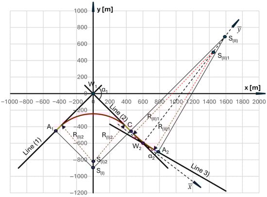
Figure 7. The determined geometric system of reverse arcs with transition curves in the local coordinate system.

After transferring the obtained solution to the PL-2000 system, using Equations (8) and (9), the situation shown in Figure 8 arises.

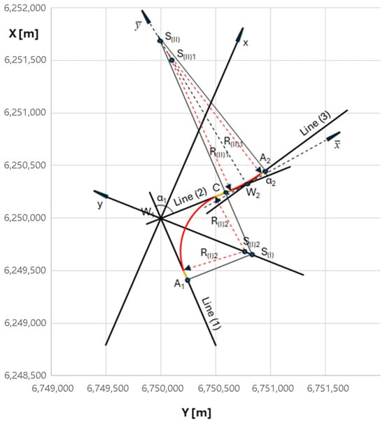
Figure 8. Designated geometric system of reverse arcs with transition curves in the PL-2000 coordinate system.

9. Evaluation of the Obtained Solution

To evaluate the geometric system shown in Figure 7 and Figure 8, it is necessary to first determine its horizontal curvature along its length and then analyze the achievable train speed. The curvature diagram was based on the model of a moving rigid base of a rail vehicle, as used in Section 5. Figure 9 shows the curvature diagram for the resulting reverse curve system.

Figure 9. Graph of horizontal curvature along the length of the determined geometric system of reverse arcs from Figure 7 and Figure 8.

The curvature diagram in Figure 9 indicates that both horizontal curves can be considered independently, and the train speed on the entire system will be determined by the curve with the greater curvature (i.e., the arc with radius R_(I)2. The first step is to check the possible speed without the use of cant. This is shown in Table 6, separately for both curves under consideration. The formulas for accelerations a_m1 and a_m2 from Section 5 (taking into account the corrected radii) and the formulas for the acceleration increase

$${\psi }_1={\displaystyle \frac{a_{m1}\cdot V}{3.6\cdot l_{(I)i}}}, {\psi }_2={\displaystyle \frac{a_{m2}\cdot V}{3.6\cdot l_{(II)i}}}.$$

Table 6. Determination of train speeds in the absence of cant for both corrected curves.

Arc with Radius R(I)2					Arc with Radius R(II)1
V [km/h]	R(I)2 [m]	L(I)2 [m]	am1 [m/s2]	ψ1 [m/s3]	V [km/h]	R(II)1 [m]	L(II)1 [m]	am2 [m/s2]	ψ2 [m/s3]
60	585.697	100	0.47427	0.10945	90	1421.338	50	0.43973	0.30443
65	585.697	100	0.55661	0.13915	95	1421.338	50	0.48994	0.35804
70	585.697	100	0.64553	0.17380	100	1421.338	50	0.54287	0.41759
75	585.697	100	0.74105	0.21376	105	1421.338	50	0.59852	0.48342
80	585.697	100	0.84314	0.25943	110	1421.338	50	0.65688	0.55582
85	585.697	100	0.95183	0.31118	115	1421.338	50	0.71795	0.63511
90	585.697	100	1.06711	0.36938	120	1421.338	50	0.78174	0.72160
95	585.697	100	1.18897	0.43443	125	1421.338	50	0.84824	0.81561
100	585.697	100	1.31741	0.50670	130	1421.338	50	0.91745	0.91745
105	585.697	100	1.45249	0.58657	135	1421.338	50	0.98939	1.02744
110	585.697	100	1.59407	0.67441	140	1421.338	50	1.06403	1.14588

Table 6 shows the values of key kinematic parameters and the resulting speed derived from them. For both circular arcs, the differential impact of acceleration and acceleration increase on the achieved speed is evident. On the arc with a smaller radius (i.e., Arc I), the acceleration parameter plays a decisive role, determining V_max = 80 km/h. The acceleration gain condition would result in V_max = 100 km/h, but the lower value is valid. On the curve with a larger radius (i.e., Arc II), the opposite occurs: the acceleration gain plays a decisive role, determining V_max = 105 km/h (the acceleration condition would result in V_max = 125 km/h). Of course, on the entire reverse curve system, in the absence of cant, the determined speed is V_max = 80 km/h.

In the next step, the effects of applying cant to an arc will be examined. Table 7 presents the appropriate procedure for a circular curve with a smaller radius. The following formula for unbalanced acceleration was used:

$$a_{m1}={\displaystyle \frac{V^2}{{\left(3.6\right)}^2{R}_{(I)i}}}-g{\displaystyle \frac{h_1}{s}},$$

where h₁—cant value in millimeters, g—acceleration of gravity (g = 9.81 m/s²), s—center distance of rails (on standard gauge lines, s = 1500 mm).

Table 7. Determining the train speed for the corrected first curve, along with the selection of the cant value.

h1 [mm]	V [km/h]	R(I)2 [m]	L(I)2 [m]	am1 [m/s2]	ψ1 [m/s3]	f1 [mm/s]
120	105	585,697	100	0.66765	0.26963	35.00000
120	110	585,697	100	0.80927	0.34238	36.66667
120	115	585,697	100	0.95748	0.42350	38.33333
120	120	585,697	100	1.11228	0.51336	40.00000
130	105	585,697	100	0.60225	0.24322	37.91667
130	110	585,697	100	0.74387	0.31471	39.72222
130	115	585,697	100	0.89208	0.39457	41.52778
130	120	585,697	100	1.04688	0.48317	43.33333
130	125	585,697	100	1.20826	0.58089	45.13889
140	110	585,697	100	0.67847	0.28705	42.77778
140	115	585,697	100	0.82668	0.36565	44.72222
140	120	585,697	100	0.98148	0.45299	46.66667
140	125	585,697	100	1.14286	0.54945	48.61111
140	130	585,697	100	1.31083	0.65541	50.55556
145	110	585,697	100	0.64577	0.27321	44.30556
145	115	585,697	100	0.79398	0.35118	46.31944
145	120	585,697	100	0.94878	0.43790	48.33333
145	125	585,697	100	1.11016	0.53373	50.34722

The key kinematic parameter values and the resulting speed are bolded.

The formula for the increase in acceleration ψ₁ is the same as that used in Table 6, but the lifting speed of the rolling stock wheel on the gradient due to cant must be determined using the formula

$$f_1={\displaystyle \frac{h_1\cdot V}{3.6\cdot L_{(I)i}}}.$$

The f₁ value should not be greater than 50 mm/s [35].

As it turns out, this speed is determined by the unbalanced acceleration occurring on the curve. The highest achievable speed on Arc I is 115 km/h, with an applied cant of 140 mm. For this speed, all required kinematic conditions are met.

A similar procedure performed for Arc II is illustrated in Table 8. The designation h₂ refers to the cant value on this curve. The following calculation formulas were used:

$$a_{m2}={\displaystyle \frac{V^2}{{\left(3.6\right)}^2{R}_{(II)i}}}-g{\displaystyle \frac{h_2}{s}}, {\psi }_2={\displaystyle \frac{a_{m2}\cdot V}{3.6\cdot L_{(II)i}}}, f_2={\displaystyle \frac{h_2\cdot V}{3.6\cdot L_{(II)i}}}.$$

Table 8. Determining the train speed for the corrected second curve, along with the selection of the cant value.

h2 [mm]	V [km/h]	R(II)1 [m]	L(II)1 [m]	am2 [m/s2]	ψ2 [m/s3]	f2 [mm/s]
20	105	1,421,338	50	0.46772	0.37777	11.66667
20	110	1,421,338	50	0.52608	0.44514	12.22222
20	115	1,421,338	50	0.58715	0.51940	12.77778
20	120	1,421,338	50	0.65094	0.60086	13.33333
20	125	1,421,338	50	0.71744	0.68984	13.88889
20	130	1,421,338	50	0.78665	0.78665	14.44444
20	135	1,421,338	50	0.85859	0.89161	15.00000
30	110	1,421,338	50	0.46068	0.38980	18.33333
30	115	1,421,338	50	0.52175	0.46155	19.13337
30	120	1,421,338	50	0.58554	0.54050	20.00000
30	125	1,421,338	50	0.65204	0.62696	20.83333
30	130	1,421,338	50	0.72125	0.72125	21.66667
30	135	1,421,338	50	0.79319	0.82369	22.50000
30	140	1,421,338	50	0.86783	0.93459	23.33333
40	115	1,421,338	50	0.45635	0.40369	25.55556
40	120	1,421,338	50	0.52014	0.48013	26.66667
40	125	1,421,338	50	0.58664	0.56408	27.77778
40	130	1,421,338	50	0.65585	0.65585	28.88889
40	135	1,421,338	50	0.72779	0.75578	30.00000
40	140	1,421,338	50	0.80243	0.86416	31.11111
40	145	1,421,338	50	0.87979	0.98130	32.22222
45	115	1,421,338	50	0.42365	0.37477	28.75000
45	120	1,421,338	50	0.48744	0.44994	30.00000
45	125	1,421,338	50	0.55394	0.53263	31.25000
45	130	1,421,338	50	0.62315	0.62315	32.50000
45	135	1,421,338	50	0.69509	0.72182	33.75000
45	140	1,421,338	50	0.76973	0.82894	35,00000
45	145	1,421,338	50	0.84709	0.94483	36.25000
45	150	1,421,338	50	0.92716	1.06980	37.50000
50	115	1,421,338	50	0.39095	0.34584	31.94444
50	120	1,421,338	50	0.45454	0.41976	33.33333
50	125	1,421,338	50	0.52124	0.50119	34.72222
50	130	1,421,338	50	0.59045	0.59045	36.11111
50	135	1,421,338	50	0.66239	0.68786	37.50000
50	140	1,421,338	50	0.73703	0.79372	38.88889
50	145	1,421,338	50	0.81439	0.90836	40.27778
50	150	1,421,338	50	0.89446	1.03207	41.66667

The key kinematic parameter values and the resulting speed are bolded.

In Table 8, unlike Table 7, the speed is determined by the acceleration increase on the transition curve. The highest speed achieved in this analysis on Arc II is 120 km/h, with a cant of 45 mm. Of course, this speed could be significantly increased by further increasing the cant on the curve. However, this would not make much sense, as the speed on the reverse curves will be determined by the speed on the arc with a smaller radius anyway. Therefore, in the case under consideration, trains could run at 115 km/h.

To summarize the analysis of the achievable train speeds presented in this article, the effects of subsequent actions can be identified for the geometric system under consideration. In the absence of transition curves and cant on the arc, the speed is very limited, and the value of V = 60 km/h given in Table 2 is highly questionable. The use of transition curves allows for increasing this value to V = 80 km/h. Finally, the introduction of cant on the circular arc (and therefore also a gradient due to cant) determines the speed of V = 115 km/h. Higher train speeds increase the capacity of the railway line and bring specific economic benefits.

The presented procedure is universal and can be applied to other geometric situations involving the design of reverse curves. For a given layout of the main directions of a railway line, it allows for the selection of the initial radii of both circular curves, which can then be adjusted by introducing transition curves of varying lengths. The basic criterion for evaluating the resulting solution is the train speed, which can be changed by making appropriate corrections to the geometric layout.

10. Conclusions

On railway lines, due to competitive conditions with other transport systems, the most important issues currently seem to be those related to increasing train speeds; this is reflected in the dominance of high-speed rail. Traditional, existing railway lines (mostly built in the 19th century) are often overlooked in research, as they would need to be modified to meet contemporary requirements. This is particularly true for railway lines running through difficult terrain (e.g., mountainous terrain), which feature small horizontal arc radii and controversial geometric configurations such as compound curves and reverse curves. Improving the quality of these lines, leading to increased speeds, requires appropriate modernization activities.

This article addresses the design of reverse curves: a geometric system composed of two circular arcs (usually with different radii) oriented in opposite directions and directly connected. The goal is also to be able to recreate (i.e., model) an existing geometric system with reverse curves, so that subsequent corrections to the horizontal ordinates in the area where the circular arcs connect can be made. An effective design method needs to be developed that can be used not only to determine the coordinates of a new reverse curve but also to model the existing system (with a view to its subsequent modification). In the case of an existing system, measurement data obtained in the PL-2000 system can be transferred to the local coordinate system and processed there in order to determine the basic geometric parameters.

The solution to the problem is obtained analytically. Individual elements of the geometric system are described using mathematical equations, and the design itself is performed in the appropriate local Cartesian coordinate system, based on the symmetrically arranged adjacent main directions of the route. However, in the case of reverse curves, there is a fundamental difference from most analytical design methods. In geometric systems, two adjacent main directions are most often identified and incorporated into further procedures (including the creation of a local coordinate system). In reverse curves, a third main direction appears, significantly complicating the matter, limiting the universality of the developed method. However, with regard to the local coordinate system, the adopted principle was retained: it is determined using two adjacent main directions. The origin of this system is located at its intersection, the coordinates of which are known in the global coordinate system.

The radii of the reverse arcs must correspond to the existing system of main directions. The key issue here is to select the correct connection point for both arcs. Therefore, reverse arcs cannot be arbitrarily shaped; various conditions must be taken into account. Entering the determined arcs into the system of main directions allows for the creation of the initial geometric system of the reverse arcs. Then, transition curves are introduced for both existing circular arcs. This is possible if there is an appropriate distance between the points of intersection of the main directions (which cannot be too small). As a result, the arc radii are reduced. Their values are determined iteratively. The corresponding calculation procedure for the first arc takes place in the local coordinate system, while the procedure for the second arc takes place in the auxiliary coordinate system, with the resulting solution subsequently transferred to the local coordinate system.

This article presents a set of formulas for creating a geometric system of reverse curves. These formulas were used in the calculation example. A graph of the horizontal curvature of the track axis and a method for determining train speed are shown. The train speed on the entire system is determined by the curve with the greatest curvature. In the first stage, the achievable speed without the use of cant on the curve was determined. Next, the effects of applying cant were discussed. The presented procedure is universal and can be applied to other geometric situations involving the design of reverse curves.

When modeling an existing geometric system and using survey data, the coordinates of the W₁ main point in the PL-2000 coordinate system are naturally subject to a certain error, which affects the local coordinate system and, consequently, the entire calculation process. However, the determination of the designed geometric system in the field will also be subject to error. Therefore, the error will not be generated solely by the calculation phase of the process. The final accuracy will depend on the precision of the measurement (geodetic) technique used.

The presented method enables full control over the reverse curve design process and allows for strategic decision-making regarding the optimal geometric system parameters. It allows for the use of both freely accepted input data and measurement data from the operating railway track. After the calculation procedure is completed in the local coordinate system, data is generated for the establishment of a new geometric system in the field.

References

- Beria, P.; Grimaldi, R.; Albalate, D.; Bel, G. Delusions of success: Costs and demand of high-speed rail in Italy and Spain. Transp. Policy 2018, 68, 63–79. [Google Scholar] [CrossRef]
- Yang, X.; Lin, S.; Zhang, J.; He, M. Does high-speed rail promote enterprises productivity? Evidence from China. J. Adv. Transp. 2019, 2019, 1279489. [Google Scholar] [CrossRef]
- De Rus, G. The economic rationale for high-speed rail. In International Encyclopedia of Transportation; Elsevier: Amsterdam, The Netherlands, 2021. [Google Scholar]
- Xiao, F.; Wang, J.; Du, D. High-speed rail heading for innovation: The impact of HSR on intercity technology transfer. Area Dev. Policy 2022, 7, 293–311. [Google Scholar] [CrossRef]
- Chen, H.; Zhu, T.; Zhao, L. High-speed railway opening, industrial symbiotic agglomeration and green sustainable development—Empirical evidence from China. Sustainability 2024, 16, 2070. [Google Scholar] [CrossRef]
- Bigi, F.; Bosi, T.; Pineda-Jaramillo, J.; Viti, F. Long-term fleet management for freight trains: Assessing the impact of wagon maintenance through simulation of shunting policies. J. Rail Transp. Plan. Manag. 2024, 29, 100430. [Google Scholar] [CrossRef]
- Wang, Q.; Jiang, X.; Zeng, J.; Mao, R.; Wei, L.; Wu, S. Innovative method for high-speed railway carbody vibration control caused by hunting instability using underframe suspended equipment. J. Vib. Control. 2024, 31, 3245–3257. [Google Scholar] [CrossRef]
- Zhang, M.; Hu, R.; Mo, J.; Xiang, Z.; Zhou, Z. A cross-domain state monitoring method for high-speed train brake pads based on data generation under small sample conditions. Measurement 2024, 226, 114074. [Google Scholar] [CrossRef]
- Qazi, A.; Yin, H.; Sebès, M.; Chollet, H.; Pozzolini, C. A semi-analytical numerical method for modelling the normal wheel-rail contact. Veh. Syst. Dyn. 2022, 60, 1322–1340. [Google Scholar]
- Fang, C.; Jaafar, S.A.; Zhou, W.; Yan, H.; Chen, J.; Meng, X. Wheel-rail contact and friction models: A review of recent advances. Proc. Inst. Mech. Eng. F J. Rail Rapid Transit 2023, 237, 1245–1259. [Google Scholar] [CrossRef]
- Wu, B.; Yang, Y.; Xiao, G. A transient three-dimensional wheel-rail adhesion model under wet condition considering starvation and surface roughness. Wear 2024, 540–541, 205263. [Google Scholar] [CrossRef]
- Kasimu, A.; Zhou, W.; Yan, H.; Wang, Y.; Shen, C. Evaluation of the vehicle-cargo and vehicle-trackside clearance of long and big railway freight vehicles. Alex. Eng. J. 2025, 119, 22–34. [Google Scholar]
- Wang, Z.; Wu, B.; Wu, S.; Wen, Z. Effects of wheel tread hollow wear on wheel-rail adhesion under wet condition. Tribol. Int. 2025, 211, 110927. [Google Scholar] [CrossRef]
- AutoCAD Civil 3D: Design, Engineering and Construction Software. Available online: http://www.autodesk.pl/products/civil-3d (accessed on 31 August 2025).
- Bentley Rail Track: Rail Infrastructure Design and Optimization. Available online: https://www.bentley.com/software/rail-design (accessed on 31 August 2025).
- Koc, W. Elements of Track Systems Design Theory; Gdansk University of Technology Publishing House: Gdansk, Poland, 2004. Available online: https://mostwiedzy.pl/pl/publication/elementy-teorii-projektowania-ukladow-torowych.92886-1 (accessed on 6 January 2026). (In Polish).
- Hodas, S. Design of railway track for speed and high-speed railways. Procedia Eng. 2014, 91, 256–261. [Google Scholar] [CrossRef]
- Aghastya, A.; Prihatanto, R.; Rachman, N.F.; Adi, W.T.; Astuti, S.W.; Wirawan, W.A. A new geometric planning approach for railroads based on satellite imagery. AIP Conf. Proc. 2023, 2671, 50005. [Google Scholar] [CrossRef]
- Guerrieri, M. Fundamentals of Railway Design, Chapter: The Alignment Design of Ordinary and High-Speed Railways; Springer: Berlin/Heidelberg, Germany, 2023; pp. 21–56. [Google Scholar]
- Tasci, L.; Kuloglu, N. Investigation of a new transition curve. Balt. J. Road Bridge Eng. 2011, 6, 23−29. [Google Scholar]
- Kobryn, A. Universal solutions of transition curves. J. Surv. Eng. 2016, 142, 4016010. [Google Scholar] [CrossRef]
- Koc, W. New transition curve adapted to railway operational requirements. J. Surv. Eng. 2019, 145, 4019009. [Google Scholar] [CrossRef]
- Zboinski, K.; Woznica, P. Optimum railway transition curves for different circular arc radii. Arch. Civ. Eng. 2022, 68, 111–125. [Google Scholar] [CrossRef]
- Palsson, B.A. Design of optimization of switch rails in railway turnouts. Veh. Syst. Dyn. 2013, 51, 1610–1639. [Google Scholar] [CrossRef]
- Ping, W. Design of High-Speed Railway Turnouts; Theory and Applications; Elsevier Science & Technology: Oxford, UK, 2015. [Google Scholar]
- Koc, W. Analytical method of connecting parallel tracks located in a circular arc using curved turnouts. J. Transp. Eng. Part A Syst. 2020, 146, 4019081. [Google Scholar] [CrossRef]
- Hamarat, M.; Papaelias, M.; Kaewunruen, S. Fatigue damage assessment of complex railway turnout crossings via Peridynamics-based digital twin. Sci. Rep. 2022, 12, 14377. [Google Scholar] [CrossRef]
- Tonias, E.C.; Tonias, C.N. Compound and reversed curves. In Geometric Procedures for Civil Engineers; Springer International Publishing AG: Cham, Germany, 2016; pp. 185–242. [Google Scholar]
- Koc, W. Design of reverse curves adapted to the satellite measurements. Adv. Civ. Eng. 2016, 2016, 6503962. [Google Scholar] [CrossRef]
- Koc, W. Analytical method of modelling the geometric system of communication route. Math. Probl. Eng. 2014, 2014, 679817. [Google Scholar] [CrossRef]
- Regulation of the Council of Ministers of 15 October 2012 on the National Spatial Reference System. J. Laws Repub. Pol. 2012. Available online: https://api.sejm.gov.pl/eli/acts/DU/2024/342/text.pdf (accessed on 6 January 2026). (In Polish)
- Koc, W. Determination of track axis coordinates in the analytical method of designing railway route geometry. Eur. J. Appl. Sci. 2024, 12, 339–362. [Google Scholar] [CrossRef]
- Koc, W. Modeling of compound curves on railway lines. Geomatics 2025, 5, 21. [Google Scholar] [CrossRef]
- Korn, G.A.; Korn, T.M. Mathematical Handbook for Scientists and Engineers, 1st ed.; McGraw–Hill Book Company: New York, NY, USA, 1968. [Google Scholar]
- Technical Standards—Detailed technical conditions for the modernization or construction of railway lines up to a speed of Vmax ≤ 250 km/h. In Volume I—Railroad—Appendix ST-T1-A6—Geometric Layouts of Tracks; PKP Polish Railway Lines S.A.: Warszawa, Poland, 2021; Available online: https://www.plk-sa.pl/klienci-i-kontrahenci/akty-prawne-i-przepisy/standardy-techniczne (accessed on 6 January 2026). (In Polish)
- Regulation of the Minister of Transport and Maritime Economy of 10 September 1998 on the Technical Conditions to Be Met by Railway Structures and Their Location. J. Laws Repub. Pol. 1998. Available online: https://serwisppoz.tarbonus.pl/wp-content/uploads/R980987p.pdf (accessed on 6 January 2026). (In Polish).
Disclaimer/Publisher’s Note: The statements, opinions and data contained in all publications are solely those of the individual author(s) and contributor(s) and not of MDPI and/or the editor(s). MDPI and/or the editor(s) disclaim responsibility for any injury to people or property resulting from any ideas, methods, instructions or products referred to in the content. |
© 2026 by the author. Licensee MDPI, Basel, Switzerland. This article is an open access article distributed under the terms and conditions of the Creative Commons Attribution (CC BY) license.