Quantum Kinetic Theory of the Spin Hall Effect for Disordered Graphene with Rashba Spin–Orbit Coupling

Abstract

The spin Hall effect for the model Hamiltonian of graphene with Rashba spin–orbit coupling is analyzed by means of a recently derived quantum kinetic theory of the linear response for multi-band electron systems. The latter expresses the interband part of the density matrix in terms of the intraband occupation numbers, which can be obtained as solutions of a Boltzmann transport equation. The analysis, which, in the case of the model here considered, can be carried out in a completely analytical way, thus provides an effective pedagogical illustration of the general theory. While our results agree with those previously obtained with alternative approaches for the same model, our comparatively simpler and more physically transparent derivation illustrates the advantages of our formalism when dealing with non trivial multi-band Hamiltonians.

1. Introduction

Recently, we have derived a linear response (LR) formula for weakly disordered multi-band electron systems [1], within the context of the Keldysh non-equilibrium quantum field theory. This result has extended to disordered systems the derivation of the quantum kinetic theory initially obtained for pure multi-band electron systems [2]. Graphene [3] and van der Waals heterostructures [4], where the spin–orbit coupling (SOC) may be proximized by transition-metal dichalcogenides (TMDs) [5,6], have been over the last decade an intensive field of research because it is an ideal platform for spintronics [7,8,9,10,11,12,13,14,15]. It has been pointed out that the proximized SOC can be effectively described by the usual graphene continuum Hamiltonian [16] with the addition of a Rashba term [17,18]. For brevity, we refer to this model as the Dirac–Rashba model, emphasizing the linear-in-momentum spectrum and the SOC due to reduced symmetry. Other SOC terms may also be added depending of the specific reduced symmetry induced by the nearby TMD [6,9].

The spin Hall effect and the current-induced spin polarization (CISP) have been theoretically studied by means of the Kubo formula within the Matsubara Green’s function approach [19,20,21,22,23,24,25], the Eilenberger quasi-classical Green’s function approach [26], the Boltzmann Equation [27], first-principle calculations [28,29], and density-functional theory [30]. The Dirac–Rashba model is, therefore, an ideal case for testing the efficiency of our LR formula, also considering the increasing importance of this model and its generalizations for van der Waals heterostructures [31,32,33].

The model enjoys particle–hole symmetry in the sense that the spectrum is invariant by the inversion of the Fermi energy ${\epsilon }_F$ with respect to the Dirac point. In the following, for the sake of definiteness, we will focus on the case of the Fermi level at positive energy. Furthermore, as it will be shown in the following, the model has two distinct physical regimes depending on the strength of the SOC constant with respect to the Fermi energy. In particular, regime I is characterized by the Fermi level intersecting only one band, whereas in regime II two bands cross the Fermi level. In both cases, the symmetry of the Rashba SOC requires the vanishing of the spin Hall current in the bulk for a uniform and stationary electric field [20]. This implies an exact compensation of the intrinsic spin Hall current originating from the non trivial Berry phase by disorder corrections, with some disorder scattering being necessary to insure a steady state in presence of an electric field. Such exact compensation has been found previously to occur in the 2D electron gas [34,35,36]. To capture this key effect in the diagrammatic approach one needs to include the so-called vertex corrections [20], whose algebraic complexity grows very fast with the number of bands involved. In [1], a direct connection between our LR formula and the Kubo formula in the Matsubara formalism has been proven, in the sense that each term of our formula has a counterpart in the diagrammatic language, with our LR formalisms capturing the vertex corrections in the ladder approximation. As we are able to show below, the two distinct physical regimes referred to above are both described by our LR formula once one has taken into account the proper solution of the Boltzmann equation. We will show here that the two regimes indicated above differ by the way the disorder scattering gives rise to the electron self-energy for a multi-band Hamiltonian. In regime II, when all possible bands cross the Fermi level, the (anti-hermitian part of the) electron self-energy is proportional to the identity in the Hilbert space upon which the multi-band Hamiltonian is acting. This is no longer the case in regime I. In the language of our LR formula, the two regimes are then characterized by the vanishing or not of the term directly connected to the electron self-energy. In our opinion, the rich physical behavior of the Dirac–Rashba model illustrates well how our LR formula can be used and then provides a benchmark for applying it to more challenging multi-band Hamiltonians.

Our aim is to keep a pedagogical tone in our discussion, which will have the following layout. In the Section 2, we summarize and briefly explain our quantum kinetic formulation of the LR. In Section 3, we introduce the model Hamiltonian and illustrate its spectrum and eigenstate structure. In Section 4, we start applying our formula, with a first step consisting in the resolution of the Boltzmann system of equations for the band occupation numbers. The latter are used as an input for the evaluation of the spin Hall conductivity, which is carried out in Section 5. Finally, in Section 6, we conclude and provide some outlook for further applications of our formalism.

2. The Linear Response Formula

Let us assume a multi-band $N\times N$ Hamiltonian matrix $\widehat{h}\left(\mathbf{p}\right)$ with $\mathbf{p}$ the kinetic electron pseudomomentum. Such an Hamiltonian matrix can be a “toy” model or an effective low-energy approximation of a realistic Hamiltonian. In the following sections we will specialize to the Dirac–Rashba model, but for the time being we do not need to specify it further. We also assume a weak static disorder in the form of a dilute random distribution of point scattering potentials treated at the level of the self-consistent second Born approximation. The disorder potential is taken to be delta-correlated, i.e., $⟨V\left(\mathbf{x}\right)V\left({\mathbf{x}}^{\prime }\right)⟩=n_i{v}_0^2\delta (\mathbf{x}-{\mathbf{x}}^{\prime })$, where $⟨\cdots ⟩$ indicates the average over the random distribution, $n_i$ is the impurity concentration, and $v_0$ the scattering amplitude. Then, the LR for the gauge invariant Wigner function [37] is obtained as [1]:

$${\hat{\rho }}^{\left(1\right)}=\sum _n{f}_n^{\left(1\right)}{\hat{P}}_n+\sum _{n\ne m}{\hat{\rho }}_{nm}^{\left(1\right)},$$

(1)

with ${\widehat{P}}_n$ the projector into the eigenspace associated with the eigenvalue ${\epsilon }_n$ of $\widehat{h}$ [38] i.e., associated with the $\mathrm{n}$th band of the system. The key property and usefulness of the gauge invariant Wigner function [37,39] is that it yields the expectation value of any single particle observable, $\hat{O}$, in the form of its local density, $⟨{\rho }_o⟩\left(x\right)$, as a trace of its Weyl symbol $\widehat{o}(\mathbf{x},\mathbf{p})$:

$$⟨{\rho }_o⟩\left(x\right)=\int {\displaystyle \frac{d^{d}p}{{(2\pi \hslash )}^d}}\mathrm{Tr}\left[\widehat{\rho }(x,\mathbf{p})\widehat{o}(\mathbf{x},\mathbf{p})\right].$$

(2)

The $f_n^{\left(1\right)}$ are the occupation number functions in momentum space for the different bands, while the off-diagonal components ${\widehat{\rho }}_{nm}^{\left(1\right)}={\widehat{P}}_n{\widehat{\rho }}^{\left(1\right)}{\widehat{P}}_m$ encode the interband quantum coherences. At the level of the LR to an external electric field, the occupation number functions are solution of the following system of coupled linear Boltzmann Equations (here below $n_{FD}\left({\epsilon }_n\right)$ is the equilibrium Fermi–Dirac distribution for the n-th energy band):

$${\partial }_t{f}_n+{\mathbf{v}}_n·{\partial }_{\mathit{x}}{f}_n+e\mathit{E}·{\partial }_{\mathit{p}}{n}_{FD}\left({\epsilon }_n\right)=I_n,$$

(3)

with the collision integral for the n-th equation given by

$$I_n=\sum _m{\int }_{\underset{˜}{\mathbf{p}}}\delta \left({\tilde{\epsilon }}_m-{\epsilon }_n\right)W_{nm}\left({\underset{˜}{f}}_m-f_n\right),$$

(4)

where, for later notational convenience,

$${\int }_{\underset{˜}{\mathbf{p}}}\equiv \int {\displaystyle \frac{d^d\underset{˜}{p}}{{(2\pi \hslash )}^d}}$$

and where the scattering kernel between bands n and m reads

$$W_{nm}={\displaystyle \frac{2\pi n_i{v}_0^2}{\hslash }}\mathrm{Tr}\left[{\widehat{P}}_n{\underset{˜}{\overset{^}{P}}}_m\right].$$

(5)

$f_n$ and ${\underset{˜}{f}}_m$ depend on momenta $\mathbf{p}$ and $\underset{˜}{\mathbf{p}}$, respectively. In the spatially uniform case, the solution of Equation (3) with its full collision integral is completely equivalent to the intraband part of the LR in the Kubo diagrammatic formalism with vertex corrections in the ladder approximation, as shown in [1,40]. Once the occupation numbers $f_n$ are known, the off-diagonal components of the density matrix are obtained as [1]

$$\begin{array}{cc}\hfill {\widehat{\rho }}_{nm}^{\left(1\right)}=& -\mathbf{i}\hslash \left[{\displaystyle \frac{n_{FD}\left({\epsilon }_n\right)-n_{FD}\left({\epsilon }_m\right)}{{\epsilon }_n-{\epsilon }_m}}\left(e\mathit{E}\right)+{\displaystyle \frac{1}{2}}{\partial }_{\mathit{x}}\left(f_n+f_m\right)\right]·\left({\partial }_{\mathit{p}}{\widehat{P}}_n\right){\widehat{P}}_m-{\displaystyle \frac{\mathbf{i}\hslash }{2({\epsilon }_n-{\epsilon }_m)}}{\displaystyle \frac{2\pi n_i{v}_0^2}{\hslash }}\times \cdots \hfill \\ \hfill \cdots \times & \sum _q{\int }_{\underset{˜}{\mathbf{p}}}\left[\delta \left({\tilde{\epsilon }}_q-{\epsilon }_n\right)\left({\underset{˜}{f}}_q-f_n\right)+\delta \left({\tilde{\epsilon }}_q-{\epsilon }_m\right)\left({\underset{˜}{f}}_q-f_m\right)\right]{\widehat{P}}_n{\underset{˜}{\overset{^}{P}}}_q{\widehat{P}}_m.\hfill \end{array}$$

(6)

The above formula shows that the off-diagonal components of the Wigner function appear as “slave variables”, in the sense that they are entirely determined from the occupation numbers $f_n$. Taken together, Equations (3) and (6) provide a $U\left(1\right)\times SU\left(N\right)$ gauge invariant quantum geometric decomposition of the LR between the occupation number functions and the off-diagonal components of the Wigner function. In this article, we will use Equation (6) to study the transverse spin Hall current response to a uniform and static electric field in the limit of an infinite system. The latter assumption simply means that we will not be concerned with boundary effects. This allows us to neglect the explicit consideration of the gradient term in the first square brackets of Equation (6). The first term in the square brackets of Equation (6) has the form of the LR for a pure system in the absence of disorder scattering. This term, which we will refer to as the intrinsic term, is responsible for instance for the quantum geometric contribution to the Hall conductivity, found to be a topological invariant [41]. The introduction of disorder, as long as the Fermi level lies in an energy gap, does not affect it or yields subleading corrections in a power expansion in the impurity concentration. The second term, which contains the impurity concentration is due to disorder. We will refer to this term as the disorder term. This term contains the occupation numbers $f_n$, which are the solution of the Boltzmann system (3) above. As we will see in detail later on, the $f_n$ scale with the inverse of impurity concentration, so that the disorder-induced term of Equation (6) is actually independent of the impurity concentration and remains finite in the limit of vanishing disorder. As shown in the diagrammatic approach [19,20,22], the spin Hall conductivity of the pure system, which is clearly independent of the impurity concentration, is exactly canceled by the vertex corrections induced by the disorder scattering. These vertex corrections manifest, in the present formalism, in the disorder term of the Formula (6). Further details about this quantum kinetic formulation of the LR, and its the derivation, can be found in [1] and we will not repeat them here. Nevertheless, we want to emphasize that our Equations (3) and (6) can be directly used for any multi-band electron system, starting from the sole knowledge of the free electron Hamiltonian $\widehat{h}\left(\mathbf{p}\right)$ assumed to provide a reasonable description of its electronic structure in the vicinity of the Fermi level. In the following Sections we will illustrate, with the consideration of the Dirac–Rashba model, how the above Equations (3) and (6) can be used in practice to evaluate a specific physical observable, namely the spin Hall current.

3. The Hamiltonian of the Dirac–Rashba Model

The Hamiltonian of graphene (at fixed valley), in the presence of Rashba spin–orbit coupling, reads

$$\widehat{h}\left(\mathbf{p}\right)=v\mathsf{\sigma }{s}_0·\mathbf{p}+\lambda ({\sigma }_1{s}_2-{\sigma }_2{s}_1),\lambda >0,$$

(7)

where $\mathsf{\sigma }$ and $\mathbf{s}$ are two sets of Pauli matrices describing graphene-lattice and spin degrees of freedom and ${\sigma }_i{s}_j$ is a Kronecker product. ${\sigma }_0$ and $s_0$ indicate the identity matrix for lattice and spin degrees of freedom. In the following, we set $v=1$ for simplicity. The above Hamiltonian has four eigenvalues, ${\epsilon }_n$, which are labeled as follows

$${\epsilon }_1=-\lambda -{\mu }_p,{\epsilon }_2=\lambda -{\mu }_p,{\epsilon }_3=-\lambda +{\mu }_p,{\epsilon }_4=\lambda +{\mu }_p,$$

(8)

where ${\mu }_p\equiv \sqrt{p^2+{\lambda }^2}$. The energy band ${\epsilon }_n$ are displayed in Figure 1.

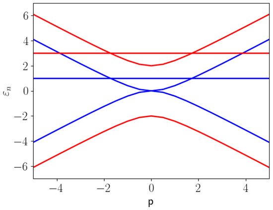
Figure 1. Energy bands of the Dirac–Rashba model. The blue and red horizontal straight lines mark the Fermi level for regimes I and II, respectively. In the plot, we set $\lambda =1$.

A Dirac point occurs at the origin in momentum space, where bands (in blue in Figure 1) ${\epsilon }_2$ and ${\epsilon }_3$ meet. Conversely, bands ${\epsilon }_1$ and ${\epsilon }_4$ only exist at energy ${\epsilon }_F<-2\lambda$ or ${\epsilon }_F>2\lambda$, respectively. The region of energies $(-2\lambda ,2\lambda )$ is sometimes called the pseudo-gap.

We now consider the form of the projectors which are necessary to evaluate the LR formula discussed in the previous Section. By indicating with $\varphi$ the angle between the momentum $\mathbf{p}$ and the x axis, the n-th eigenvector reads [19,20]

$$|n,\mathbf{p}⟩={\beta }_n{\left({(-1)}^{n+1}\mathbf{i}{e}^{-\mathbf{i}\varphi },{\alpha }_n,{(-1)}^{n+1}\mathbf{i}{\alpha }_n,e^{\mathbf{i}\varphi }\right)}^T,$$

(9)

where

$${\alpha }_n={\displaystyle \frac{{\epsilon }_n}{p}},{\beta }_n={\displaystyle \frac{p}{2\sqrt{{\mu }_p\left|{\epsilon }_n\right|}}}.$$

(10)

The projectors are obtained as ${\widehat{P}}_n=|n,\mathbf{p}⟩⟨n,\mathbf{p}|$ and read

$${\widehat{P}}_n={\beta }_n^2\left(\begin{array}{cccc}1,& {(-1)}^{n+1}\mathbf{i}{e}^{-\mathbf{i}\varphi }{\alpha }_n,& e^{-\mathbf{i}\varphi }{\alpha }_n,& {(-1)}^{n+1}\mathbf{i}{e}^{-2\mathbf{i}\varphi }\\ {(-1)}^n\mathbf{i}{e}^{\mathbf{i}\varphi }{\alpha }_n,& {\alpha }_n^2,& {(-1)}^n\mathbf{i}{\alpha }_n^2,& e^{-\mathbf{i}\varphi }{\alpha }_n\\ e^{\mathbf{i}\varphi }{\alpha }_n,& {(-1)}^{n+1}\mathbf{i}{\alpha }_n^2& {\alpha }_n^2,& {(-1)}^{n+1}\mathbf{i}{e}^{-\mathbf{i}\varphi }{\alpha }_n\\ {(-1)}^n\mathbf{i}{e}^{2\mathbf{i}\varphi },& e^{\mathbf{i}\varphi }{\alpha }_n,& {(-1)}^n\mathbf{i}{e}^{\mathbf{i}\varphi }{\alpha }_n,& 1\end{array}\right).$$

(11)

One can easily check that ${\sum }_n{\widehat{P}}_n=1$. Notice that our choice of phase for the eigenvector (9) is irrelevant because our formula is expressed in the terms of the projectors, which are invariant with respect to the choice of the phase. In the actual calculations, in the following, we will transform a trace over projectors into products of matrix elements of the observables taken between the eigenstates (9). The insensitivity to the phase choice remains however guaranteed, since the initial formula is expressed in terms of the projectors.

The projectors can be easily expanded in terms of the set of matrices ${\sigma }_i{s}_j$ [20]. We will not do this here because it is not necessary. However, in Appendix A, we do provide the expansion for the angle average of the projectors, which will be needed in the evaluation of the LR formula. We also point out that all relevant physical observables can be defined in terms of the set of matrices ${\sigma }_i{s}_j$. For instance, the electrical current flowing along the x axis is given by ${\sigma }_1{s}_0$ and the spin current flowing along the y axis and with spin polarization along the z axis is given by $(\hslash /2){\sigma }_2{s}_3$. In Appendix B, we provide the expression of the matrix elements of several observables.

For the sake of definiteness, we take the chemical potential ${\epsilon }_F>0$ (cf. Figure 1). Due to the symmetry of the energy spectrum (8), the case for ${\epsilon }_F<0$ can be easily obtained. We also notice that for ${\epsilon }_F>0$, there are two distinct regimes. We have regime I, when $0<{\epsilon }_F<2\lambda$ and only band ${\epsilon }_3$ crosses the Fermi level (marked by a blue horizontal line in Figure 1). Regime II occurs when ${\epsilon }_F>2\lambda$ and both bands ${\epsilon }_3$ and ${\epsilon }_4$ cross the Fermi level (marked by a red horizontal line in Figure 1).

4. The Solution of the Boltzmann Equation for the Occupation Numbers

In order to solve the Boltzmann equation for the distribution functions $f_n$, we will need the square of the absolute value of the overlap between eigenstates at different momenta ($\varphi$ and $\underset{˜}{\varphi }$, being the angles of $\mathbf{p}$ and $\underset{˜}{\mathbf{p}}$ with the x axis and $\Delta \varphi =\varphi -\underset{˜}{\varphi }$). By using the result (A15) in Appendix B, we have

$$|⟨n\mathbf{p}|m\underset{˜}{\mathbf{p}}⟩{|}^2=4{\left({\beta }_n{\underset{˜}{\beta }}_m\right)}^2\left[{({\alpha }_n{\underset{˜}{\alpha }}_m+cos(\varphi -\underset{˜}{\varphi }))}^2{\delta }_{m+n,2k}+{sin}^2(\varphi -\underset{˜}{\varphi }){\delta }_{m+n,2k+1}\right].$$

(12)

This immediately allows us to derive the scattering kernel matrix (5) as

$$W_{nm}(\varphi -\underset{˜}{\varphi })={\displaystyle \frac{2\pi n_i{v}_0^2}{\hslash }}{\displaystyle \frac{1}{4}}\left(\begin{array}{cc}{\displaystyle \frac{{((2\lambda +{\epsilon }_F)cos(\varphi -\underset{˜}{\varphi })+{\epsilon }_F)}^2}{{({\epsilon }_F+\lambda )}^2}}& {\displaystyle \frac{\left({\epsilon }_F^2-4{\lambda }^2\right){sin}^2(\varphi -\underset{˜}{\varphi })}{({\epsilon }_F^2-{\lambda }^2)}}\\ {\displaystyle \frac{\left({\epsilon }_F^2-4{\lambda }^2\right){sin}^2(\varphi -\underset{˜}{\varphi })}{{({ϵ}_F^2-\lambda )}^2}}& {\displaystyle \frac{{(({\epsilon }_F-2\lambda )cos(\varphi -\underset{˜}{\varphi })+{\epsilon }_F)}^2}{{({\epsilon }_F-\lambda )}^2}}\end{array}\right),$$

(13)

where the momenta $\mathbf{p}$ and $\underset{˜}{\mathbf{p}}$ are evaluated at the Fermi level for the two bands, i.e., $p_{F,3}=\sqrt{{\epsilon }_F({\epsilon }_F+2\lambda )}$ and $p_{F,4}=\sqrt{{\epsilon }_F({\epsilon }_F-2\lambda )}$ when ${\epsilon }_F>2\lambda$ in regime II. When ${\epsilon }_F<2\lambda$, in regime I, we have only one Fermi momentum $p_{F,3}=\sqrt{{\epsilon }_F({\epsilon }_F+2\lambda )}$. Notice how diagonal (off-diagonal) matrix elements of $W_{nm}$ correspond to even (odd) combinations of $n+m$. To this end, we have introduced the notation with the Kronecker symbol ${\delta }_{n+m,2k}$, meaning that the sum of n and m is an even integer with k an integer. Similarly ${\delta }_{n+m,2k+1}$ means that $n+m$ is an odd number. The presence of these Kronecker symbols in the matrix elements defines an important way in which the model behaves and we will rely heavily on this to simplify our calculations.

In the presence of a static and uniform electric field and in the regime of degeneracy of the Fermi gas, the system of Boltzmann Equations (3) reduces to

$$-\left(e\mathit{E}\right)·{\partial }_{\mathit{p}}{\epsilon }_n\delta ({\epsilon }_n-{\epsilon }_F)=\sum _m{\int }_{\underset{˜}{\mathbf{p}}}\delta \left({\underset{˜}{\epsilon }}_m-{\epsilon }_n\right)W_{nm}\left({\underset{˜}{f}}_m-f_n\right),$$

(14)

which can be solved by iteration. We observe that ${\partial }_{\mathbf{p}}{\epsilon }_n={\partial }_p{\epsilon }_n\widehat{\mathbf{p}}\equiv v_n\widehat{\mathbf{p}}$, with $\widehat{\mathbf{p}}=({\widehat{p}}_x,{\widehat{p}}_y)\equiv (cos\left(\varphi \right),sin\left(\varphi \right))$ the unit vector in the direction of the momentum $\mathbf{p}$. The solutions of the system (14), with the electric field taken along the x axis for the sake of definiteness, can be sought in the form

$$f_n=-e{E}_x{\widehat{p}}_x{\displaystyle \frac{\hslash }{2\pi n_i{v}_0^2}}\delta ({\epsilon }_n-{\epsilon }_F){\overline{f}}_n,$$

(15)

where ${\overline{f}}_n$ is a Fermi surface constant for the energy band ${\epsilon }_n$. The equation for the functions ${\overline{f}}_n$ reads

$$v_n=\sum _m{D}_m{\int }_0^{2\pi }{\displaystyle \frac{\mathrm{d}\underset{˜}{\varphi }}{2\pi }}{\overline{W}}_{nm}(\varphi -\underset{˜}{\varphi })(cos(\varphi -\underset{˜}{\varphi }){\overline{f}}_m-{\overline{f}}_n),$$

(16)

where we have introduced the density of states at the Fermi level of the n-th energy band

$$D_n={\int }_{\mathbf{p}}\delta ({\epsilon }_n-{\epsilon }_F),$$

(17)

and ${\overline{W}}_{nm}=(\hslash /2\pi n_i{v}_0^2)W_{nm}$. Explicitly, the expressions for the velocities and the densities of states at the Fermi level are, in both regimes I and II,

$$v_3={\displaystyle \frac{\sqrt{{\epsilon }_F({\epsilon }_F+2\lambda )}}{{\epsilon }_F+\lambda }},v_4={\displaystyle \frac{\sqrt{{\epsilon }_F({\epsilon }_F-2\lambda )}}{{\epsilon }_F-\lambda }},D_3={\displaystyle \frac{{\epsilon }_F+\lambda }{2\pi {\hslash }^2}},D_4={\displaystyle \frac{{\epsilon }_F-\lambda }{2\pi {\hslash }^2}}.$$

(18)

In order to solve Equation (16), we need the following averages

$${\int }_0^{2\pi }{\displaystyle \frac{\mathrm{d}\underset{˜}{\varphi }}{2\pi }}{\overline{W}}_{nm}(\varphi -\underset{˜}{\varphi })={\displaystyle \frac{1}{4}}\left[\begin{array}{cc}{\displaystyle \frac{{\epsilon }_F^2+{({\epsilon }_F+2\lambda )}^2/2}{{({\epsilon }_F+\lambda )}^2}}& {\displaystyle \frac{{\epsilon }_F^2-{\lambda }^2}{2({\epsilon }_F^2-{\lambda }^2)}}\\ {\displaystyle \frac{{\epsilon }_F^2-{\lambda }^2}{2({\epsilon }_F^2-{\lambda }^2)}}& {\displaystyle \frac{{\epsilon }_F^2+{({\epsilon }_F-2\lambda )}^2/2}{{({\epsilon }_F-\lambda )}^2}}\end{array}\right]$$

(19)

and

$${\int }_0^{2\pi }{\displaystyle \frac{\mathrm{d}\underset{˜}{\varphi }}{2\pi }}cos(\varphi -\underset{˜}{\varphi }){\overline{W}}_{nm}(\varphi -\underset{˜}{\varphi })={\displaystyle \frac{1}{4}}\left[\begin{array}{cc}{\displaystyle \frac{{\epsilon }_F({\epsilon }_F+2\lambda )}{{({\epsilon }_F+\lambda )}^2}}& 0\\ 0& {\displaystyle \frac{{\epsilon }_F({\epsilon }_F-2\lambda )}{{({\epsilon }_F-\lambda )}^2}}\end{array}\right].$$

(20)

The last equation shows that, in fact, the system (16) actually decouples in independent equations. For the solution of Equation (16), we must discuss separately the two regimes I and II. In regime I, we have only one equation with solution

$${\overline{f}}_3=-16\pi {\hslash }^2{\displaystyle \frac{p_{F,3}}{{\epsilon }_F^2+4{\lambda }^2}}.$$

(21)

In regime II, we have instead

$${\overline{f}}_3=-8\pi {\hslash }^2{\displaystyle \frac{p_{F,3}}{{\epsilon }_F^2}},{\overline{f}}_4=-8\pi {\hslash }^2{\displaystyle \frac{p_{F,4}}{{\epsilon }_F^2}}.$$

(22)

Notice how the expression for ${\overline{f}}_3$ is continuous at the value ${\epsilon }_F=2\lambda$ when moving from regime I to regime II. Once obtained the occupation numbers in the presence of the electric field, we can insert them into the expression (6) for the off-diagonal part of the density matrix. This will be done in the next Section.

5. The Interband Density Matrix and the Evaluation of the Spin Hall Conductivity

We evaluate the spin Hall conductivity ${\sigma }^{sH}$ by considering the first and third term in Equation (6). The Weyl symbol for the spin current flowing along the y axis (recall that the electric field has been taken along the x axis) and with spin polarization along the z axis reads

$${\widehat{J}}_y^z={\displaystyle \frac{\hslash }{2}}{\sigma }_2{s}_3.$$

(23)

Specifically, we write ($n\ne m$)

$${⟨J_y^z⟩}^{\left(int\right)}={\displaystyle \frac{\hslash }{2}}\sum _{n,m}{\int }_{\mathbf{p}}\mathrm{Tr}\left[{\widehat{\rho }}_{nm}^{\left(int\right)}{\sigma }_2{s}_3\right]\equiv {\sigma }^{sH,int}{E}_x$$

(24)

for the intrinsic part and

$${⟨J_y^z⟩}^{\left(dis\right)}={\displaystyle \frac{\hslash }{2}}\sum _{n,m}{\int }_{\mathbf{p}}\mathrm{Tr}\left[{\widehat{\rho }}_{nm}^{\left(dis\right)}{\sigma }_2{s}_3\right]\equiv {\sigma }^{sH,dis}{E}_x$$

(25)

for the disorder-induced part. Here, ${\sigma }^{sH,int}$ and ${\sigma }^{sH,dis}$ denote the intrinsic and disorder contributions, respectively.

5.1. The Geometry-Induced Intrinsic Term

In the presence of a uniform and static electric field, the intrinsic term reduces to the first term in the first square brackets of Equation (6). We have

$${\sigma }^{sH,int}=\mathbf{i}{\displaystyle \frac{e{\hslash }^2}{4}}\sum _{n\ne m}{\int }_{\mathbf{p}}{\displaystyle \frac{n_{FD}\left({\epsilon }_n\right)-n_{FD}\left({\epsilon }_m\right)}{{\epsilon }_n-{\epsilon }_m}}\mathrm{Tr}\left[{\sigma }_2{s}_3\left({\partial }_{p_x}{\widehat{P}}_n\right){\widehat{P}}_m\right].$$

(26)

By noting the projectors relation with $n\ne m$

$$\left({\partial }_{p_x}{\widehat{P}}_n\right){\widehat{P}}_m={\displaystyle \frac{1}{{\epsilon }_n-{\epsilon }_m}}{\widehat{P}}_n\left({\partial }_{p_x}\widehat{h}\left(\mathbf{p}\right)\right){\widehat{P}}_m$$

(27)

we get

$${\sigma }^{sH,int}=\mathbf{i}{\displaystyle \frac{e{\hslash }^2}{4}}\sum _{n\ne m}{\int }_{\mathbf{p}}{\displaystyle \frac{n_{FD}\left({\epsilon }_n\right)-n_{FD}\left({\epsilon }_m\right)}{{({\epsilon }_n-{\epsilon }_m)}^2}}\mathrm{Tr}\left[{\sigma }_2{s}_3{\widehat{P}}_n{\sigma }_1{s}_0{\widehat{P}}_m\right].$$

(28)

By using the expression of the matrix elements evaluated in Appendix B, we have

$${\sigma }^{sH,int}=\mathbf{i}{\displaystyle \frac{e{\hslash }^2}{4}}\sum _{n\ne m}{\int }_{\mathbf{p}}{\displaystyle \frac{n_{FD}\left({\epsilon }_n\right)-n_{FD}\left({\epsilon }_m\right)}{{({\epsilon }_n-{\epsilon }_m)}^2}}{I}_{mn}^{23}{I}_{nm}^{10}.$$

(29)

The only dependence on the direction of the momentum $\mathbf{p}$ comes from the matrix elements $I_{mn}^{23}$ (cf. Equation (A14)) and $I_{mn}^{10}$ (cf. Equation (A12)). We may then perform the angle integration at once

$${\int }_0^{2\pi }{\displaystyle \frac{\mathrm{d}\varphi }{2\pi }}{I}_{mn}^{23}{I}_{mn}^{10}=4\mathbf{i}{\left({\beta }_m{\beta }_n\right)}^2({\alpha }_m^2-{\alpha }_n^2).$$

(30)

After recalling the expression for ${\alpha }_n$ and ${\beta }_n$ (cf. Equation (10)), we obtain

$${\sigma }^{sH,int}={\displaystyle \frac{e{\hslash }^2}{16}}\sum _{n\ne m}{\int }_{\mathbf{p}}{\displaystyle \frac{n_{FD}\left({\epsilon }_n\right)-n_{FD}\left({\epsilon }_m\right)}{({\epsilon }_n-{\epsilon }_m)}}{\displaystyle \frac{{\epsilon }_m+{\epsilon }_n}{{\mu }_p^2}}.$$

(31)

From the above expression, it is clear that there can be no terms involving pairs of band related by particle-hole symmetry such as the pair with bands ${\epsilon }_1$ and ${\epsilon }_4$ or the pair with bands ${\epsilon }_2$ and ${\epsilon }_3$. Furthermore, regime I is defined by $n_{FD}\left({\epsilon }_1\right)=n_{FD}\left({\epsilon }_2\right)=1$, $n_{FD}\left({\epsilon }_4\right)=0$ and $n_{FD}\left({\epsilon }_3\right)=\theta ({\epsilon }_F-{\epsilon }_3)$. Instead in regime II, one has $n_{FD}\left({\epsilon }_1\right)=n_{FD}\left({\epsilon }_2\right)=1$, and $n_{FD}\left({\epsilon }_3\right)=\theta ({\epsilon }_F-{\epsilon }_3)$, $n_{FD}\left({\epsilon }_4\right)=\theta ({\epsilon }_F-{\epsilon }_4)$. In performing the momentum integration, it is useful to make the change of variable $\mu d\mu =pdp$ and, by considering the pairs $(n,m)=(1,3),(2,4),(3,4)$ and adding an extra factor of 2 to keep track of the terms with the indices n and m interchanged, we obtain in regime II

$${\sigma }^{sH,int}={\displaystyle \frac{e}{16\pi }}\left(\lambda {\int }_{{\epsilon }_F+\lambda }^{\infty }{\displaystyle \frac{d\mu }{{\mu }^2}}-\lambda {\int }_{{\epsilon }_F-\lambda }^{\infty }{\displaystyle \frac{d\mu }{{\mu }^2}}-{\displaystyle \frac{1}{\lambda }}{\int }_{{\epsilon }_F-\lambda }^{{\epsilon }_F+\lambda }d\mu \right),$$

(32)

where the three integrals in round brackets correspond to pairs of band $(1,3)$, $(2,4)$ and $(3,4)$, respectively. In regime I, we have instead, because $\mu >\lambda >0$ and ${\epsilon }_F-\lambda <0$,

$${\sigma }^{sH,int}={\displaystyle \frac{e}{16\pi }}\left(\lambda {\int }_{{\epsilon }_F+\lambda }^{\infty }{\displaystyle \frac{d\mu }{{\mu }^2}}-\lambda {\int }_{\lambda }^{\infty }{\displaystyle \frac{d\mu }{{\mu }^2}}-{\displaystyle \frac{1}{\lambda }}{\int }_{\lambda }^{{\epsilon }_F+\lambda }d\mu \right).$$

(33)

Hence

$$\begin{array}{ccc}\hfill {\sigma }^{sH,int}& =& -{\displaystyle \frac{e}{16\pi }}{\displaystyle \frac{{\epsilon }_F({\epsilon }_F+2\lambda )}{\lambda ({\epsilon }_F+\lambda )}},\mathrm{Regime}\mathrm{I}:{\epsilon }_F<2\lambda \hfill \end{array}$$

(34)

$$\begin{array}{ccc}\hfill {\sigma }^{sH,int}& =& -{\displaystyle \frac{e}{8\pi }}{\displaystyle \frac{{\epsilon }_F^2}{{\epsilon }_F^2-{\lambda }^2}}\mathrm{Regime}\mathrm{II}:{\epsilon }_F>2\lambda .\hfill \end{array}$$

(35)

Equations (34) and (35) reproduce the well-known result for the spin Hall conductivity in the absence of disorder [20,42].

5.2. The Disorder-Induced Term

We now focus our attention on the term induced by disorder. By using the ansatz (15), we obtain ($\varphi$ and $\underset{˜}{\varphi }$, being the angles of $\mathbf{p}$ and $\underset{˜}{\mathbf{p}}$ with the x axis)

$$\begin{array}{ccc}\hfill {\sigma }^{sH,dis}& =& \mathbf{i}{\displaystyle \frac{e{\hslash }^2}{4}}{\int }_{\mathbf{p}}{\int }_{\underset{˜}{\mathbf{p}}}\sum _{n,m,q}{\eta }_{nm}{\underset{˜}{\delta }}_{F,q}\left[{\delta }_{F,n}(\underset{˜}{c}{\overline{f}}_q-c{\overline{f}}_n)+{\delta }_{F,m}(\underset{˜}{c}{\overline{f}}_q-c{\overline{f}}_m)\right]\mathrm{Tr}\left[{\sigma }_2{s}_3{\widehat{P}}_n{\underset{˜}{\overset{^}{P}}}_q{\widehat{P}}_m\right],\hfill \end{array}$$

where ${\delta }_{F,n}\equiv \delta ({\epsilon }_n-{\epsilon }_F)$, ${\eta }_{nm}={({\epsilon }_n-{\epsilon }_m)}^{-1}$, $\underset{˜}{c}=cos\left(\underset{˜}{\varphi }\right)$, $c=cos\left(\varphi \right)$. It is convenient to split the above contribution in the form

$${\sigma }^{sH,dis}={\sigma }_A+{\sigma }_B,$$

(36)

where

$${\sigma }_A=\mathbf{i}{\displaystyle \frac{e{\hslash }^2}{4}}{\int }_{\mathbf{p}}{\int }_{\underset{˜}{\mathbf{p}}}\sum _{n,m,q}{\eta }_{nm}{\underset{˜}{\delta }}_{F,q}\underset{˜}{c}{\overline{f}}_q\left[{\delta }_{F,n}+{\delta }_{F,m}\right]\mathrm{Tr}\left[{\sigma }_2{s}_3{\widehat{P}}_n{\underset{˜}{\overset{^}{P}}}_q{\widehat{P}}_m\right]$$

(37)

and

$${\sigma }_B=-\mathbf{i}{\displaystyle \frac{e{\hslash }^2}{4}}{\int }_{\mathbf{p}}{\int }_{\underset{˜}{\mathbf{p}}}\sum _{n,m,q}{\eta }_{nm}{\underset{˜}{\delta }}_{F,q}c\left[{\delta }_{F,n}{\overline{f}}_n+{\delta }_{F,m}{\overline{f}}_m\right]\mathrm{Tr}\left[{\sigma }_2{s}_3{\widehat{P}}_n{\underset{˜}{\overset{^}{P}}}_q{\widehat{P}}_m\right].$$

(38)

The reason for this splitting is motivated by the fact the integration over the momentum $\underset{˜}{\mathbf{p}}$ contains a factor $\underset{˜}{c}$ in the case of ${\sigma }_A$, whereas such a factor does not appear for ${\sigma }_B$. Then the two terms involve different angle averages of the projector ${\underset{˜}{\overset{^}{P}}}_q$ under the trace symbol. By using the result of Appendix A, we have

$${\int }_{\underset{˜}{\mathbf{p}}}{\underset{˜}{\delta }}_{F,q}\underset{˜}{c}{\underset{˜}{\overset{^}{P}}}_q={\displaystyle \frac{p_{F,q}\mathrm{sign}\left({\epsilon }_F\right)}{16\pi {\hslash }^2}}({\sigma }_1{s}_0+{(-1)}^q{\sigma }_0{s}_2),$$

(39)

and

$${\int }_{\underset{˜}{\mathbf{p}}}{\underset{˜}{\delta }}_{F,q}{\underset{˜}{\overset{^}{P}}}_q={\displaystyle \frac{1}{8\pi {\hslash }^2}}\left[({\epsilon }_F+{(-1)}^{q+1}\lambda ){\sigma }_0{s}_0+{(-1)}^{q+1}\left(\lambda {\sigma }_3{s}_3-{\displaystyle \frac{{\epsilon }_F}{2}}({\sigma }_1{s}_2-{\sigma }_2{s}_1)\right)\right].$$

(40)

In the first equation above, $p_{F,q}$ is the Fermi momentum of the energy band ${\epsilon }_q$. Hence, in regime I, we may have only the term with $q=3$ in the sum, whereas in regime II, we have $q=3$ and $q=4$. In the second equation above, the terms with the factor ${(-1)}^{q+1}$ cancel in the sum over q in regime II. This implies that in regime II, the second equation yields a term proportional to the identity matrix. In the diagrammatic language [20], the integration of the projectors yields the anti-hermitian part of the retarded Green’s function self-energy. As stated in the Introduction, this corresponds to the fact that in regime II, the self-energy is proportional to the identity matrix. As a result of being proportional to the identity matrix, the product of the two projectors in Equation (38) ${\widehat{P}}_n$ and ${\widehat{P}}_m$ under the trace vanishes because of orthogonality with $n\ne m$. Hence, in regime II, ${\sigma }_B=0$ identically. We may then rewrite the two contributions ${\sigma }_A$ and ${\sigma }_B$ as

$${\sigma }_A=\mathbf{i}{\displaystyle \frac{e}{64\pi }}\sum _q\sum _{n\ne m}{\int }_{\mathbf{p}}{p}_{F,q}{\overline{f}}_q{\eta }_{nm}({\delta }_{F,n}+{\delta }_{F,m})I_{mn}^{23}(I_{nm}^{10}+{(-1)}^q{I}_{nm}^{02})$$

(41)

and

$${\sigma }_B=-\mathbf{i}{\displaystyle \frac{e}{32\pi }}\sum _q{(-1)}^{q+1}\sum _{n\ne m}{\int }_{\mathbf{p}}cos\left(\varphi \right){\eta }_{nm}({\delta }_{F,n}{\overline{f}}_n+{\delta }_{F,m}{\overline{f}}_m)I_{mn}^{23}\left(\lambda I_{nm}^{33}-{\displaystyle \frac{{\epsilon }_F}{2}}{I}_{nm}^{12-21}\right).$$

(42)

In the derivation of the last two equations, we have converted the traces in products of matrix elements and used the result of Appendix B, i.e.,

$$\mathrm{Tr}\left[{\sigma }_i{s}_j{\widehat{P}}_n{\sigma }_k{s}_l{\widehat{P}}_m\right]=I_{mn}^{ij}{I}_{nm}^{kl}.$$

(43)

In both Equations (41) and (42), we perform first the integration over the direction of the momentum $\mathbf{p}$ by defining

$$L_{mn}^q={\int }_0^{2\pi }{\displaystyle \frac{d\varphi }{2\pi }}{I}_{mn}^{23}(I_{nm}^{10}+{(-1)}^q{I}_{nm}^{02})$$

(44)

and

$$M_{mn}={\int }_0^{2\pi }{\displaystyle \frac{d\varphi }{2\pi }}cos\left(\varphi \right)I_{mn}^{23}\left(\lambda I_{nm}^{33}-{\displaystyle \frac{{\epsilon }_F}{2}}{I}_{nm}^{12-21}\right).$$

(45)

Equations (41) becomes then

$${\sigma }_A=\mathbf{i}{\displaystyle \frac{e}{32\pi }}\sum _q\sum _{n\ne m}{\int }_{\mathbf{p}}{p}_{F,q}{\overline{f}}_q{\delta }_{F,n}{\eta }_{nm}{L}_{mn}^q,$$

(46)

which has been obtained by exchanging the indices n and m and using the property ${\eta }_{mn}=-{\eta }_{nm}$ and $L_{nm}^q=-L_{mn}^q$. In the same way, Equation (42) becomes

$${\sigma }_B=-\mathbf{i}{\displaystyle \frac{e}{16\pi }}\sum _q{(-1)}^{q+1}\sum _{n\ne m}{\int }_{\mathbf{p}}{\eta }_{nm}{\delta }_{F,n}{\overline{f}}_n{M}_{mn}.$$

(47)

By using the expression of the matrix elements in Appendix B, we obtain

$$L_{mn}^q=4\mathbf{i}{\left({\beta }_m{\beta }_n\right)}^2\left[{\delta }_{n+m,2k}{\delta }_{m+q,2k}({\alpha }_m^2-{\alpha }_n^2)+{\delta }_{n+m,2k+1}({\alpha }_m+{\alpha }_n)({\delta }_{m+q,2k}{\alpha }_m-{\delta }_{m+q,2k+1}{\alpha }_n)\right]$$

(48)

and

$$M_{mn}=2\mathbf{i}{\left({\beta }_m{\beta }_n\right)}^2({\alpha }_m-{\alpha }_n)\left(\lambda (1-{\alpha }_m{\alpha }_n)-{(-1)}^n{\epsilon }_F{\alpha }_m{\alpha }_m\right){\delta }_{m+n,2k}.$$

(49)

After recalling the expression for ${\alpha }_n$ and ${\beta }_n$ in Equation (10), we have

$$L_{mn}^q=\mathbf{i}{\displaystyle \frac{1}{4{\mu }_p^2}}\left[{\delta }_{n+m,2k}{\delta }_{m+q,2k}({\epsilon }_m^2-{\epsilon }_n^2)+{\delta }_{n+m,2k+1}({\epsilon }_m+{\epsilon }_n)({\delta }_{m+q,2k}{\epsilon }_m-{\delta }_{m+q,2k+1}{\epsilon }_n)\right]$$

(50)

and

$$M_{mn}=\mathbf{i}{\displaystyle \frac{p}{8{\mu }_p^2}}({\epsilon }_m-{\epsilon }_n)\left(2\lambda +{(-1)}^n{\epsilon }_F\right){\delta }_{m+n,2k},$$

(51)

where in the last equation, we used the fact that ${\alpha }_m{\alpha }_n=1$ only if both n and m are even or odd as required from the factor ${\delta }_{m+n,2k}$. As we mentioned, the contribution due to ${\sigma }_B$ only exists in regime I, when only band ${\epsilon }_3$ crosses the Fermi level. In the expression for ${\sigma }_B$ in the sum over q and n, only the term with $q=n=3$ remains. Because of the constraint given by the factor ${\delta }_{m+n,2k}$ in the expression for $M_{mn}$, there remains only the term with $m=1$. Hence

$${\sigma }_B=-\mathbf{i}{\displaystyle \frac{e}{16\pi }}{\int }_{\mathbf{p}}{\eta }_{31}{\delta }_{F,3}{\overline{f}}_3{M}_{13}={\displaystyle \frac{e}{16\pi }}{\displaystyle \frac{p_{F,3}{\overline{f}}_3}{16\pi {\hslash }^2}}{\displaystyle \frac{{\epsilon }_F-2\lambda }{{\epsilon }_F+\lambda }},$$

(52)

which is valid only in regime I.

In order to evaluate ${\sigma }_A$ we must examine the expression of $L_{mn}^q$. In principle there may be six different pairs for the indices m and n, i.e., $(m,n)=(1,2),(1,3),(1,4),(2,3),(2,4),(3,4)$. Because the expression for $L_{mn}^q$ contains the factor ${\epsilon }_m+{\epsilon }_m$, we can exclude the pairs $(1,4)$ and $(2,3)$, as these are related by particle–hole symmetry and ${\epsilon }_m+{\epsilon }_m=0$. Then, we also observe that if both m and n are even (odd), then necessarily, q must be even (odd). This leaves only four possible combinations: $L_{13}^3$, $L_{24}^4$, $L_{34}^3$ and $L_{34}^4$, whose expressions read

$$\begin{array}{ccc}\hfill L_{13}^3& =& \mathbf{i}{\displaystyle \frac{\lambda }{{\mu }_p}}\hfill \end{array}$$

(53)

$$\begin{array}{ccc}\hfill L_{24}^4& =& -\mathbf{i}{\displaystyle \frac{\lambda }{{\mu }_p}}\hfill \end{array}$$

(54)

$$\begin{array}{ccc}\hfill L_{34}^3& =& \mathbf{i}{\displaystyle \frac{{\mu }_p-\lambda }{2{\mu }_p}}\hfill \end{array}$$

(55)

$$\begin{array}{ccc}\hfill L_{34}^4& =& -\mathbf{i}{\displaystyle \frac{{\mu }_p+\lambda }{2{\mu }_p}}.\hfill \end{array}$$

(56)

The expression for ${\sigma }_A$ is

$$\begin{array}{ccc}\hfill {\sigma }_A& =& \mathbf{i}{\displaystyle \frac{e}{32\pi }}{\int }_{\mathbf{p}}{p}_{F,3}{\overline{f}}_3\left[{\delta }_{F,3}({\eta }_{31}{L}_{13}^3+{\eta }_{34}{L}_{43}^3)+{\delta }_{F,4}{\eta }_{43}{L}_{34}^3\right]\hfill \end{array}$$

(57)

$$\begin{array}{ccc}& +& \mathbf{i}{\displaystyle \frac{e}{32\pi }}{\int }_{\mathbf{p}}{p}_{F,4}{\overline{f}}_4\left[{\delta }_{F,4}({\eta }_{42}{L}_{24}^4+{\eta }_{43}{L}_{34}^4)+{\delta }_{F,3}{\eta }_{34}{L}_{43}^4\right].\hfill \end{array}$$

(58)

Hence in regime I, we obtain

$${\sigma }_A=-{\displaystyle \frac{e}{16\pi }}{\displaystyle \frac{p_{F,3}{\overline{f}}_3}{16\pi {\hslash }^2}}\left[{\displaystyle \frac{2\lambda }{{\epsilon }_F+\lambda }}+{\displaystyle \frac{{\epsilon }_F}{\lambda }}\right],$$

(59)

while in regime II, we obtain

$${\sigma }_A=-{\displaystyle \frac{e}{16\pi }}\left[{\displaystyle \frac{p_{F,3}{\overline{f}}_3}{8\pi {\hslash }^2}}\left({\displaystyle \frac{\lambda }{{\epsilon }_F+\lambda }}+{\displaystyle \frac{{\epsilon }_F-\lambda }{\lambda }}\right)+{\displaystyle \frac{p_{F,4}{\overline{f}}_4}{8\pi {\hslash }^2}}\left(-{\displaystyle \frac{{\epsilon }_F+\lambda }{\lambda }}-{\displaystyle \frac{\lambda }{{\epsilon }_F-\lambda }}\right)\right].$$

(60)

Then in regime I, by summing ${\sigma }_A$ and ${\sigma }_B$, we have

$${\sigma }^{sH,dis}=-{\displaystyle \frac{e}{16\pi }}{\displaystyle \frac{p_{F,3}{\overline{f}}_3}{16\pi {\hslash }^2}}\left[{\displaystyle \frac{2\lambda }{{\epsilon }_F+\lambda }}+{\displaystyle \frac{{\epsilon }_F}{\lambda }}-{\displaystyle \frac{{\epsilon }_F-2\lambda }{{\epsilon }_F+\lambda }}\right]=-{\displaystyle \frac{e}{16\pi }}{\displaystyle \frac{p_{F,3}{\overline{f}}_3}{16\pi {\hslash }^2}}{\displaystyle \frac{{\epsilon }_F^2+4{\lambda }^2}{\lambda ({\epsilon }_F+\lambda )}}.$$

(61)

By recalling the expression (21) for ${\overline{f}}_3$ and that for $p_{F,3}$ one obtains the final expression for the disorder-induced contribution to the spin Hall conductivity in regime I (${\epsilon }_F<2\lambda$)

$${\sigma }^{sH,dis}={\displaystyle \frac{e}{16\pi }}{\displaystyle \frac{{\epsilon }_F({\epsilon }_F+2\lambda )}{\lambda ({\epsilon }_F+\lambda )}},$$

(62)

which is the opposite of the intrinsic contribution (34), thus yielding a zero spin Hall conductivity. It is interesting to remark that in the diagrammatic analysis of [20], the cancellation of the spin Hall conductivity in regime I is obtained after a careful consideration of the two types of contributions described by the Streda formula [43]. In the Streda formula decomposition, type-I and -II contributions refer to processes at and far away from the Fermi surface, respectively. In the present formulation, we provide a different decomposition. First, we single out the intrinsic term, which exists in the absence of disorder as well. Secondly, we describe the disorder-induced contributions both as Fermi surface terms, associated with in and out terms in kinetic equation language.

In regime II (${\epsilon }_F>2\lambda$), finally, by recalling the corresponding expressions for ${\overline{f}}_3$ and ${\overline{f}}_4$

$${\overline{f}}_3=-8\pi {\hslash }^2{\displaystyle \frac{\sqrt{{\epsilon }_F({\epsilon }_F+2\lambda )}}{{\epsilon }_F^2}},{\overline{f}}_4=-8\pi {\hslash }^2{\displaystyle \frac{\sqrt{{\epsilon }_F({\epsilon }_F-2\lambda )}}{{\epsilon }_F^2}},$$

(63)

because ${\sigma }_B=0$, we have

$${\sigma }^{sH\left(dis\right)}={\displaystyle \frac{e}{8\pi }}{\displaystyle \frac{{\epsilon }_F^2}{{\epsilon }_F^2-{\lambda }^2}},$$

(64)

which exactly cancels the intrinsic term (35). We then recover the results obtained in [20] by the diagrammatic approach. It may be worthwhile to recall that the exact cancellation of the intrinsic and disorder-induced contributions to the spin Hall conductivity is by no means accidental. In fact, in [20] it was shown that the diagrammatic result of the cancellation, while being perturbative with respect to the effect of disorder, is actually consistent with general expectations based on the Ward identities derived from the symmetry properties of the model.

6. Conclusions

In this paper, we have applied the LR formula previously derived for a multi-band Hamiltonian [1] to the case of the Dirac–Rashba model describing graphene with SOC. The model presents two distinct physical regimes depending on the position of the Fermi level. The model, though analytically tractable, presents a rich structure, which makes it an ideal testing ground for showing the usefulness of the LR formula, which, together with the solution of the Boltzmann equation for the band occupation numbers, yields the expected exact cancellation of the spin Hall conductivity for a static and uniform electric field. Although this result has been already established in the past [19,20], in our opinion, the present method is much simpler and physically transparent. Furthermore, the method presented here can be applied, perhaps with the support of numerical evaluations, to more challenging Hamiltonians [9,10,11,44,45,46,47]. These include, for instance, graphene with TMDC monolayer stacked with arbitrary twist angles [11], graphene with laterally-patterned proximity-induced SOC [9], and graphene/TMD multilayers with Rashba-engineered SOC by twist angles [10]. Furthermore, our model can be generalized to include both more complex disorder scattering and higher order terms beyond the Born approximation. To do this, one must adopt the appropriate self-energy, which appears at the initial stages of the derivation of our LR formalism from Keldysh theory [1].

References

- Valet, T.; Raimondi, R. Quantum Kinetic Theory of the Linear Response for Weakly Disordered Multiband Systems. arXiv 2024, arXiv:2410.08975. [Google Scholar]
- Valet, T.; Raimondi, R. Semiclassical kinetic theory for systems with non-trivial quantum geometry and the expectation value of physical quantities. EPL (Europhys. Lett.) 2023, 143, 26004. [Google Scholar] [CrossRef]
- Castro Neto, A.H.; Guinea, F.; Peres, N.M.R.; Novoselov, K.S.; Geim, A.K. The electronic properties of graphene. Rev. Mod. Phys. 2009, 81, 109–162. [Google Scholar] [CrossRef]
- Geim, A.; Grigorieva, I. Van der Waals heterostructures. Nature 2013, 499, 419–425. [Google Scholar] [CrossRef]
- Voiry, D.; Mohite, A.; Chhowalla, M. Phase engineering of transition metal dichalcogenides. Chem. Soc. Rev. 2015, 44, 2702–2712. [Google Scholar] [CrossRef] [PubMed]
- Kochan, D.; Irmer, S.; Fabian, J. Model spin–orbit coupling Hamiltonians for graphene systems. Phys. Rev. B 2017, 95, 165415. [Google Scholar] [CrossRef]
- Soumyanarayanan, A.; Reyren, N.; Fert, A.; Panagopoulos, C. Emergent phenomena induced by spin–orbit coupling at surfaces and interfaces. Nature 2016, 539, 509–517. [Google Scholar] [CrossRef] [PubMed]
- Han, W.; Kawakami, R.K.; Gmitra, M.; Fabian, J. Graphene spintronics. Nat. Nanotechnol. 2014, 9, 794–807. [Google Scholar] [CrossRef] [PubMed]
- Martelo, L.M.; Ferreira, A. Designer spin–orbit superlattices: Symmetry-protected Dirac cones and spin Berry curvature in two-dimensional van der Waals metamaterials. Commun. Phys. 2024, 7, 308. [Google Scholar] [CrossRef]
- Frank, T.; Faria Junior, P.E.; Zollner, K.; Fabian, J. Emergence of radial Rashba spin–orbit fields in twisted van der Waals heterostructures. Phys. Rev. B 2024, 109, L241403. [Google Scholar] [CrossRef]
- Li, Y.; Koshino, M. Twist-angle dependence of the proximity spin–orbit coupling in graphene on transition-metal dichalcogenides. Phys. Rev. B 2019, 99, 075438. [Google Scholar] [CrossRef]
- Avsar, A.; Ochoa, H.; Guinea, F.; Özyilmaz, B.; van Wees, B.J.; Vera-Marun, I.J. Colloquium: Spintronics in graphene and other two-dimensional materials. Rev. Mod. Phys. 2020, 92, 021003. [Google Scholar] [CrossRef]
- David, A.; Rakyta, P.; Kormányos, A.; Burkard, G. Induced spin–orbit coupling in twisted graphene–transition metal dichalcogenide heterobilayers: Twistronics meets spintronics. Phys. Rev. B 2019, 100, 085412. [Google Scholar] [CrossRef]
- Ahn, E. 2D materials for spintronic devices. npj 2D Mater. Appl. 2020, 4, 17. [Google Scholar] [CrossRef]
- Sierra, J.F.; Fabian, J.; Kawakami, R.K.; Roche, S.; Valenzuela, S.O. Van der Waals heterostructures for spintronics and opto-spintronics. Nat. Nanotechnol. 2021, 16, 856–868. [Google Scholar] [CrossRef]
- Peres, N.M.R. Colloquium: The transport properties of graphene: An introduction. Rev. Mod. Phys. 2010, 82, 2673–2700. [Google Scholar] [CrossRef]
- Rashba, E.I. Graphene with structure-induced spin–orbit coupling: Spin-polarized states, spin zero modes, and quantum Hall effect. Phys. Rev. B 2009, 79, 161409. [Google Scholar] [CrossRef]
- Gmitra, M.; Fabian, J. Graphene on transition-metal dichalcogenides: A platform for proximity spin–orbit physics and optospintronics. Phys. Rev. B 2015, 92, 155403. [Google Scholar] [CrossRef]
- Offidani, M.; Milletarì, M.; Raimondi, R.; Ferreira, A. Optimal Charge-to-Spin Conversion in Graphene on Transition-Metal Dichalcogenides. Phys. Rev. Lett. 2017, 119, 196801. [Google Scholar] [CrossRef]
- Milletarì, M.; Offidani, M.; Ferreira, A.; Raimondi, R. Covariant Conservation Laws and the Spin Hall Effect in Dirac-Rashba Systems. Phys. Rev. Lett. 2017, 119, 246801. [Google Scholar] [CrossRef] [PubMed]
- Offidani, M.; Raimondi, R.; Ferreira, A. Microscopic Linear Response Theory of Spin Relaxation and Relativistic Transport Phenomena in Graphene. Condens. Matter 2018, 3, 18. [Google Scholar] [CrossRef]
- Offidani, M.; Ferreira, A. Anomalous Hall Effect in 2D Dirac Materials. Phys. Rev. Lett. 2018, 121, 126802. [Google Scholar] [CrossRef]
- Baghran, R.; Tehranchi, M.M.; Phirouznia, A. Pseudo-Edelstein effect in disordered silicene. J. Phys. Condens. Matter 2021, 33, 175302. [Google Scholar] [CrossRef] [PubMed]
- Veneri, A.; Perkins, D.T.S.; Péterfalvi, C.G.; Ferreira, A. Twist angle controlled collinear Edelstein effect in van der Waals heterostructures. Phys. Rev. B 2022, 106, L081406. [Google Scholar] [CrossRef]
- Veneri, A.; Perkins, D.T.S.; Ferreira, A. Nonperturbative approach to interfacial spin–orbit torques induced by the Rashba effect. Phys. Rev. B 2022, 106, 235419. [Google Scholar] [CrossRef]
- Monaco, C.; Ferreira, A.; Raimondi, R. Spin Hall and inverse spin galvanic effects in graphene with strong interfacial spin–orbit coupling: A quasi-classical Green’s function approach. Phys. Rev. Res. 2021, 3, 033137. [Google Scholar] [CrossRef]
- Tao, L.L.; Tsymbal, E.Y. Spin-orbit dependence of anisotropic current-induced spin polarization. Phys. Rev. B 2021, 104, 085438. [Google Scholar] [CrossRef]
- Lee, S.; de Sousa, D.J.P.; Kwon, Y.K.; de Juan, F.; Chi, Z.; Casanova, F.; Low, T. Charge-to-spin conversion in twisted graphene/WSe2 heterostructures. Phys. Rev. B 2022, 106, 165420. [Google Scholar] [CrossRef]
- Chi, Z.; Lee, S.; Yang, H.; Dolan, E.; Safeer, C.K.; Ingla-Aynés, J.; Herling, F.; Ontoso, N.; Martín-García, B.; Gobbi, M.; et al. Control of Charge-Spin Interconversion in van der Waals Heterostructures with Chiral Charge Density Waves. Adv. Mater. 2024, 36, 2310768. [Google Scholar] [CrossRef]
- Rassekh, M.; Santos, H.; Latgé, A.; Chico, L.; Farjami Shayesteh, S.; Palacios, J.J. Charge-spin interconversion in graphene-based systems from density functional theory. Phys. Rev. B 2021, 104, 235429. [Google Scholar] [CrossRef]
- Cysne, T.P.; Costa, M.; Canonico, L.M.; Nardelli, M.B.; Muniz, R.B.; Rappoport, T.G. Disentangling Orbital and Valley Hall Effects in Bilayers of Transition Metal Dichalcogenides. Phys. Rev. Lett. 2021, 126, 056601. [Google Scholar] [CrossRef] [PubMed]
- Cysne, T.P.; Bhowal, S.; Vignale, G.; Rappoport, T.G. Orbital Hall effect in bilayer transition metal dichalcogenides: From the intra-atomic approximation to the Bloch states orbital magnetic moment approach. Phys. Rev. B 2022, 105, 195421. [Google Scholar] [CrossRef]
- Costa, M.; Focassio, B.; Canonico, L.M.; Cysne, T.P.; Schleder, G.R.; Muniz, R.B.; Fazzio, A.; Rappoport, T.G. Connecting Higher-Order Topology with the Orbital Hall Effect in Monolayers of Transition Metal Dichalcogenides. Phys. Rev. Lett. 2023, 130, 116204. [Google Scholar] [CrossRef]
- Raimondi, R.; Schwab, P. Spin-Hall effect in a disordered two-dimensional electron system. Phys. Rev. B 2005, 71, 033311. [Google Scholar] [CrossRef]
- Mishchenko, E.G.; Shytov, A.V.; Halperin, B.I. Spin Current and Polarization in Impure Two-Dimensional Electron Systems with Spin-Orbit Coupling. Phys. Rev. Lett. 2004, 93, 226602. [Google Scholar] [CrossRef] [PubMed]
- Inoue, J.I.; Bauer, G.E.W.; Molenkamp, L.W. Suppression of the persistent spin Hall current by defect scattering. Phys. Rev. B 2004, 70, 041303. [Google Scholar] [CrossRef]
- Serima, O.T.; Javanainen, J.; Varro, S. Gauge-independent Wigner functions: General formulation. Phys. Rev. A 1986, 33, 2913–2927. [Google Scholar] [CrossRef] [PubMed]
- Graf, A.; Piéchon, F. Berry curvature and quantum metric in N-band systems: An eigenprojector approach. Phys. Rev. B 2021, 104, 085114. [Google Scholar] [CrossRef]
- Hillery, M.; O’Connell, R.; Scully, M.; Wigner, E. Distribution functions in physics: Fundamentals. Phys. Rep. 1984, 106, 121–167. [Google Scholar] [CrossRef]
- Kim, J.; Kim, K.W.; Shin, D.; Lee, S.H.; Sinova, J.; Park, N.; Jin, H. Prediction of ferroelectricity-driven Berry curvature enabling charge- and spin-controllable photocurrent in tin telluride monolayers. Nat. Commun. 2019, 10, 3965. [Google Scholar] [CrossRef] [PubMed]
- Thouless, D.J.; Kohmoto, M.; Nightingale, M.P.; den Nijs, M. Quantized Hall Conductance in a Two-Dimensional Periodic Potential. Phys. Rev. Lett. 1982, 49, 405–408. [Google Scholar] [CrossRef]
- Dyrdał, A.; Dugaev, V.K.; Barnaś, J. Spin Hall effect in a system of Dirac fermions in the honeycomb lattice with intrinsic and Rashba spin–orbit interaction. Phys. Rev. B 2009, 80, 155444. [Google Scholar] [CrossRef]
- Streda, P. Theory of quantised Hall conductivity in two dimensions. J. Phys. C 1982, 15, L717. [Google Scholar] [CrossRef]
- Perkins, D.T.S.; Veneri, A.; Ferreira, A. Spin Hall effect: Symmetry breaking, twisting, and giant disorder renormalization. Phys. Rev. B 2024, 109, L241404. [Google Scholar] [CrossRef]
- Naimer, T.; Gmitra, M.; Fabian, J. Tuning proximity spin–orbit coupling in graphene/NbSe2 heterostructures via twist angle. Phys. Rev. B 2024, 109, 205109. [Google Scholar] [CrossRef]
- Medina Dueñas, J.; García, J.H.; Roche, S. Emerging Spin-Orbit Torques in Low-Dimensional Dirac Materials. Phys. Rev. Lett. 2024, 132, 266301. [Google Scholar] [CrossRef]
- Zhumagulov, Y.; Kochan, D.; Fabian, J. Emergent Correlated Phases in Rhombohedral Trilayer Graphene Induced by Proximity Spin-Orbit and Exchange Coupling. Phys. Rev. Lett. 2024, 132, 186401. [Google Scholar] [CrossRef]
Disclaimer/Publisher’s Note: The statements, opinions and data contained in all publications are solely those of the individual author(s) and contributor(s) and not of MDPI and/or the editor(s). MDPI and/or the editor(s) disclaim responsibility for any injury to people or property resulting from any ideas, methods, instructions or products referred to in the content. |
© 2025 by the authors. Licensee MDPI, Basel, Switzerland. This article is an open access article distributed under the terms and conditions of the Creative Commons Attribution (CC BY) license (https://creativecommons.org/licenses/by/4.0/).