Abstract
It is known that noble metals such as gold, silver and copper are not superconductors; this is also true for magnesium. This is due to the weakness of the electron–phonon interaction, which makes them excellent conductors but not superconductors. As has recently been shown for gold, silver and copper, and even for magnesium, it is possible that in very particular situations, superconductivity may occur. Quantum confinement in thin films has been consistently shown to induce a significant enhancement of the superconducting critical temperature in several superconductors. It is therefore an important fundamental question whether ultra-thin film confinement may induce observable superconductivity in non-superconducting metals such as magnesium. We study this problem using a generalization, in the Eliashberg framework, of a BCS theory of superconductivity in good metals under thin-film confinement. By numerically solving these new Eliashberg-type equations, we find the dependence of the superconducting critical temperature on the film thickness, L. This parameter-free theory predicts superconductivity in very thin magnesium films. We demonstrate that this is a fine-tuning problem where the thickness must assume a very precise value, close to half a nanometer.
1. Introduction
It has been seen that thin films of superconductors such as Pb and Al at extremely small thicknesses can produce critical temperatures considerably higher than in bulk [1] thanks to the phenomenon of quantum confinement [1,2]. We have already seen that, in this way, it is possible (theoretically) to make even noble metals in the form of very thin films become superconductors [3]. This happens because quantum confinement [4] produces an increase in the electron–phonon interaction, thanks to a larger density of states at the Fermi level. In this article, we want to demonstrate that the same theory we used previously predicts that magnesium, in the form of a very thin film, also becomes superconductor. We have already considered this topic in a paper on thin films of noble metals [3] (gold, silver, and copper). We have generalized Eliashberg’s theory in its simplest version, i.e., the one with an isotropic order parameter, high Fermi energy, and a single conduction band. To satisfy all these requirements, only three nonsuperconducting metals remain: magnesium, sodium, and potassium. But only for magnesium were all input parameters to be introduced into the Eliashberg equations known. For potassium and sodium, we have not found estimates of the Coulomb pseudopotential in the literature.
Magnesium will transition into the superconducting state at a temperature that is certainly not high but still measurable. The superconducting critical temperatures will still be low but not so low that they cannot be measured experimentally. All superconductive physical properties of old low-temperature phononic superconductors can be explained in the framework of standard one-infinite-band s-wave Eliashberg theory [5,6], essentially in the case of bulk superconductivity. All the properties of the material, in this theory, are summarized in the spectral function of electron–phonon interaction and in the Coulomb pseudopotential . Once these two quantities are known, it is possible to derive any observable of the material relating to the superconducting state. If one wants to consider the situation of extremely thin films, it is necessary to modify the standard Eliashberg theory.
When the system is no longer bulk but one dimension becomes almost negligible compared to the others (as happens, for example, in thin films), new phenomena related to quantum confinement come into play. In the context of BCS theory, Travaglino and Zaccone [2] have developed an analytical model that takes into account the thickness of the film. In this model, it is possible to reproduce the trend of the critical temperature as a function of the film thickness, as has recently been observed experimentally in lead and aluminum films. This theory is connected with the change in the Fermi surface that shows a topological transition in shape when a critical thickness is reached (here, is the concentration of free carriers). This is not exactly a topological Lifshitz transition [7], because this would involve a necking transition leading to two disconnected Fermi surfaces. Instead, in our case, there is no necking and no disconnected Fermi surfaces [2,8]. The transition is from the trivial homotopy group of the sphere (spherical or spherical-like Fermi surface) to a (still fully connected) Fermi surface that belongs to the homotopy group Z. This situation leads to a substantial modification of the electronic density of states, which, in the vicinity of the critical thickness, increases substantially and furthermore is no longer approximable by a constant around the Fermi level. This approximation is fundamental to write the Eliashberg equations in their simplest standard versions. Since we are studying very thin films, it is plausible to think that fluctuations may also play some role in the calculation of the critical temperature. Eliashberg theory is a mean field theory, and therefore, the contribution of fluctuations does not appear. Our model is , but we are close to the limit. Since, however, the Fermi energy in these systems is very high, it is possible that fluctuations are negligible and the mean-field theory provides a reasonable approximation. In future work, if we consider the effects of fluctuations we could use a new approach with holographic superconductivity to study quantum-critical fluctuations for Eliashberg’s theory [9] or to follow the Larkin–Varlamov theory of fluctuations [10]. For example, for Pb thin films, it was found [2] that Å, and this means that this effect, for metal with a high density of carriers, appears only in the case of very thin films. The theory of Travaglino and Zaccone, as we said, is written in a BCS formalism where some input parameters relating to the material do not have a clear and immediate physical interpretation, so it is better to generalize this theory in the framework of the Eliashberg theory, which is what we will show in the next section.
2. Model
In Eliashberg’s theory, the material’s physical features are taken into account via the electron–phonon spectral function and the Coulomb pseudopotential . These two quantities can be either determined experimentally or calculated from ab initio methods, especially for simple metals. In the simplest version of this theory (one isotropic-order parameter and infinite bandwidth), only two of the four terms of self-energy appear: the renormalization function and the gap function [5,6]. If Migdal’s theorem [11] is satisfied, the equations have the following mathematical expression:
n refers to integer numbers related to Matsubara energies ; is the Coulomb pseudopotential that depends, in a weak way, on a cut-off energy (, where is the maximum phonon energy); and is the Heaviside function. The electron–phonon spectral function is present inside in this way:
The strength of the electron–phonon coupling is given by the electron–phonon coupling parameter . In general, it is impossible to find exact analytical solutions of Eliashberg’s equations except for the case of extremely strong coupling () [6]. Hence, we solve them numerically with an iterative method until numerical convergence is reached. We have shown the theory in the formulation on the imaginary axis because the numerical solution is easier to find, but it also exists in the version on the real axis. In principle, the critical temperature can be calculated by solving an eigenvalue equation, but it is more simple by giving a very small test value to the superconducting gap (for example, times the value at zero temperature) and then by checking at which temperature the solution converges. In this way, it is possible to obtain a precision of that is much larger than any possible experimental verification. When we take into account the effects of quantum confinement on the free carriers, it is necessary to modify the Eliashberg theory, and the equations will be written in a more complex form, as well as increasing in number [12,13]. The effect of confinement that appears, essentially, in the normal density of states () around the Fermi level cannot be approximated by a constant value. We have already shown, in a previous article, that this new theory [1,3], devoid of free parameters, explains the increase of critical temperature [1] in the very thin films of and , as well as predicts superconductivity for , and ultra-thin films [3]. In this way, the noble metals become superconductors at precise values of film thickness L. If the is no longer a constant but a function of energy, the Eliashberg equations become slightly more complex, and they become four equations [14,15]. Another step in the generalization of the theory is to remove the infinite band approximation (which works very well for most metals in the bulk state) [12,13]. In the more general situation, we have four equations to solve [13], but in the particular case where the normal density of states is symmetrical with respect to the Fermi level (), it is possible to simplify the theory in a way in which there remain only two self-energy terms, and as before, and the new equations read as [14,15]
where and the bandwidth W is equal to half the Fermi energy, . The fact that the normal density of states is symmetric with respect to the Fermi level is a great advantage and allows us to find the numerical solution more quickly. When the effects of quantum confinement begin to manifest themselves, the NDOS can no longer be approximated by its value at the Fermi level, and two different regimes can appear [2]: and .
If we are in the case in which and, consequently, , the normal density of states has the following form
where , , , m is the electron mass, and is the Fermi energy of the bulk material. In this case, it is possible to demonstrate the following relations [2]:
with
In the regime , the has a new, linear dependence on the energy, in contrast with the standard square-root dependence that is retrieved for [2]. In order to better understand the new physics hidden in these equations, we remove the factor C, which will be put in the renormalization of the electron–phonon coupling constant.
We now recap all the changes that are present in the new Eliashberg theory:
(i) The normal density of states will no longer be a constant but a function of energy.
(ii) The electron–phonon interaction is a function of film thickness L, via because we move the prefactor of the , C, inside the definition of electron–phonon coupling as in the Coulomb pseudopotential. This choice allows one to justify the use of the Allen–Dynes equation [16] for . Of course, the shape of the electron–phonon spectral function remains the same, and we only rescale it ot change the value of electron–phonon coupling constant.
(iii) The value of the Fermi energy is also a function of the film thickness L: . Of course, in the symmetric case discussed above, it is ;
(iv) The Coulomb pseudopotential also depends on the film thickness via
where .
Instead, when and, consequently, , we have [2]
where
Now, the normal density of states is given by [2]:
The electron–phonon coupling and the Coulomb pseudopotential take, through , a dependence from the thickness:
In the standard Eliashberg equations, the reference energy is the Fermi energy, which represents the zero of energy.
In the code that numerically solves the Eliashberg equations, by recalling that the reference energy is the Fermi energy, taken as the zero of the energy, the normal density of states has been rescaled in the following way (of course, the normal density of states will be continuous for ): When and :
Instead, when and ,
3. Prediction of Critical Temperature
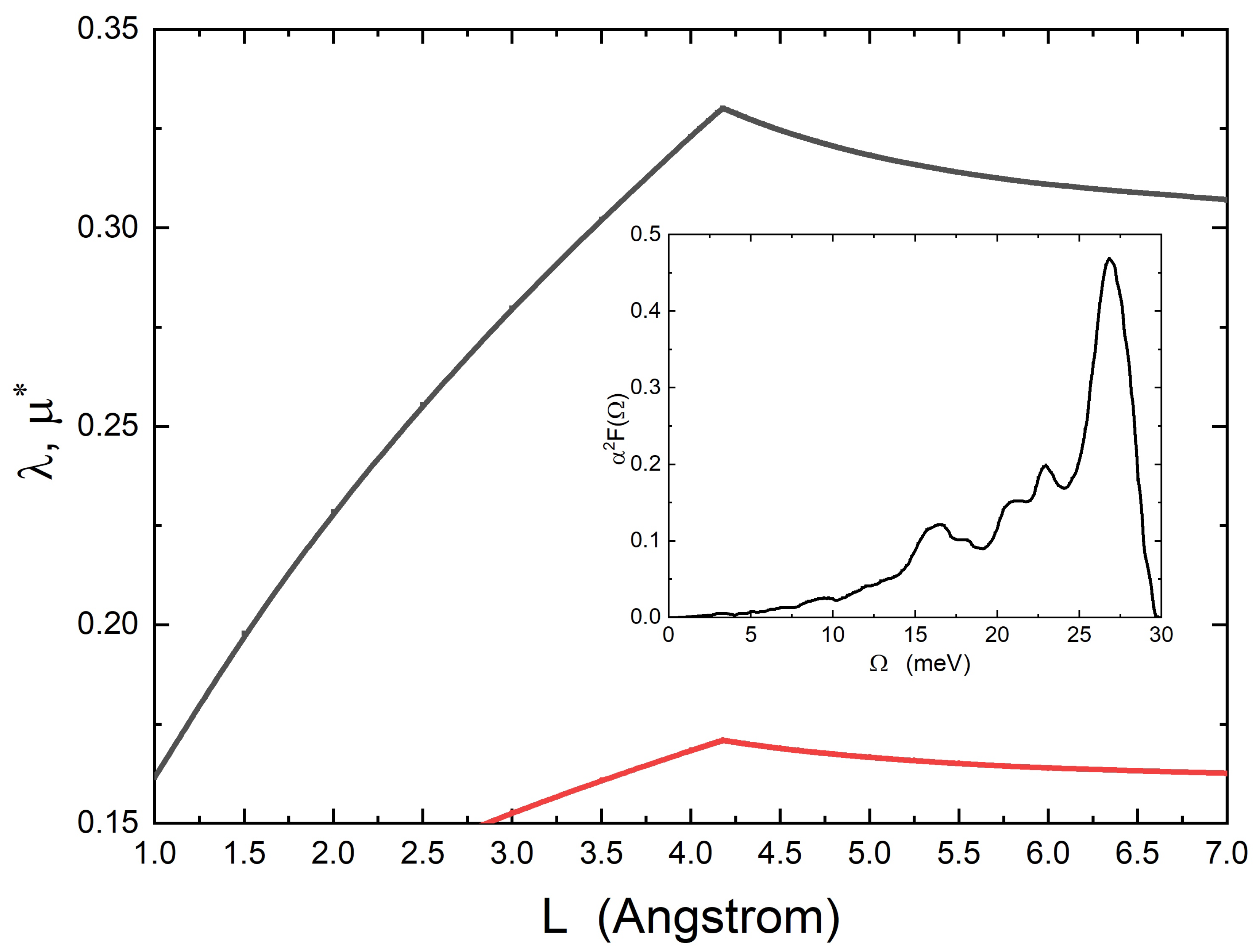
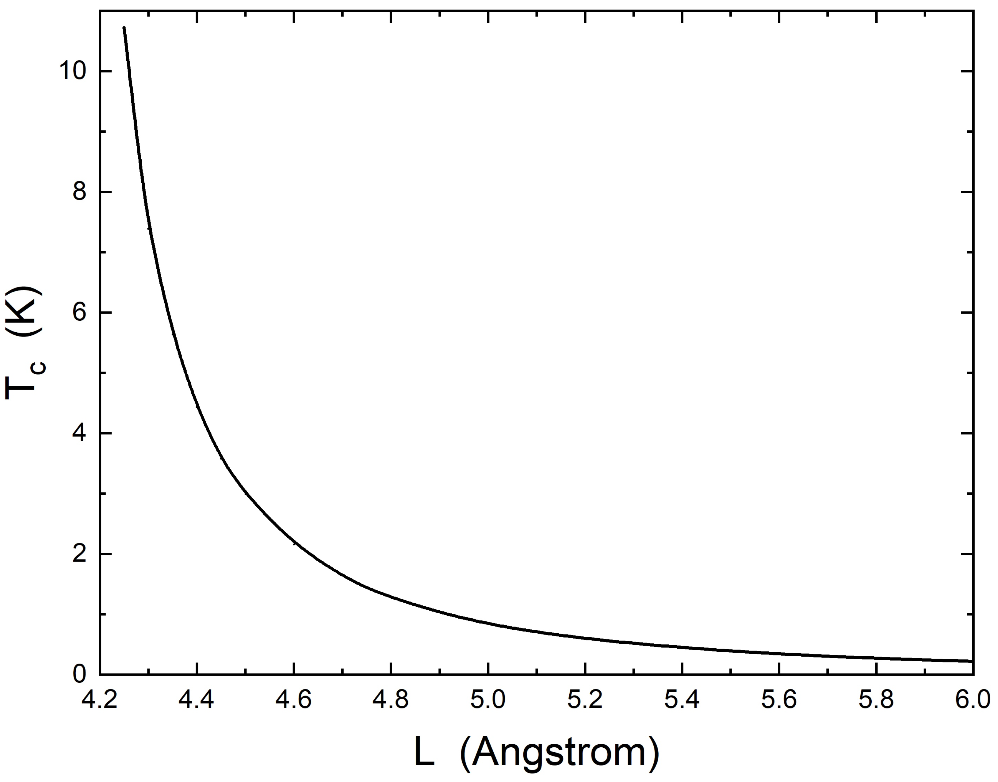
We have seen that, if the is symmetrical, the theory is simplified, and we have just two Eliashberg equations to solve. Instead, the theory becomes more complex if the is asymmetrical and there are three equations to be solved [13]. It is important to underline that the relevant fact is the nonconstant more than the symmetry of the same . Usually, the asymmetry is a problem of the second order and can become significant only in very particular situations [15]. This theory is completely general and can be easily extended to multiband metals [17,18,19,20]. As we have demonstrated in a previous article, although noble metals (, , ) have a very weak electron–phonon coupling (), they can be superconductors if they are in the shape of very thin films [3] with a thickness very close to the critical length , which is on the order of 5 Å (0.5 nm). This happens because the electron–phonon interaction is greatly enhanced and in a narrow range of thickness to produce superconductivity at experimentally accessible temperatures. The same thing happens for magnesium, as is revealed by our calculations in Figure 1, Figure 2, Figure 3 and Figure 4.
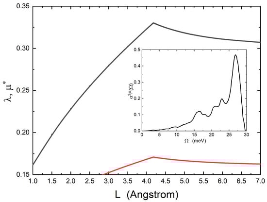
Figure 1.
Physical parameters used in the theory for magnesium films: (full black solid line) and (full red solid line). All parameters are plotted as a function of the film thickness L. In the inset, the Eliashberg electron–phonon spectral function of magnesium is shown, from ref. [21].
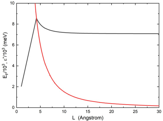
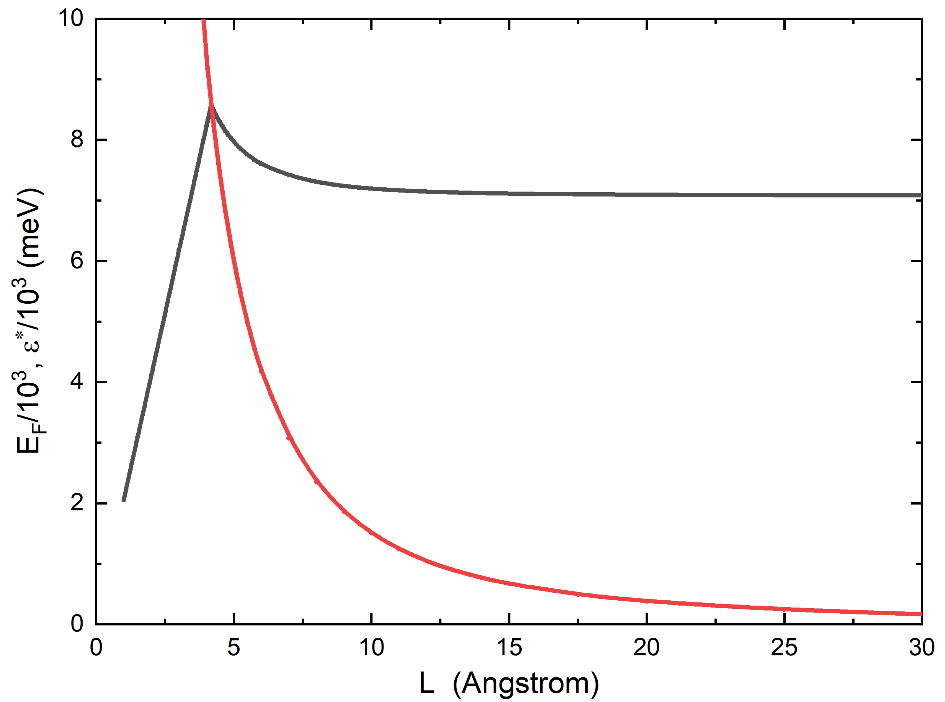
Figure 2.
Physical parameters used in the theory for magnesium films: ) (full red solid line) and (full black solid line). All parameters are plotted as a function of the film thickness L.
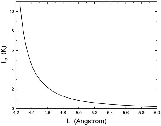
Figure 3.
Critical temperature versus film thickness L: the full solid line represents the numerical solutions of Eliashberg equations.
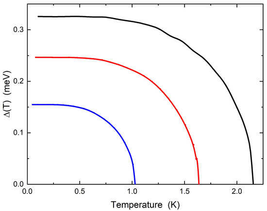
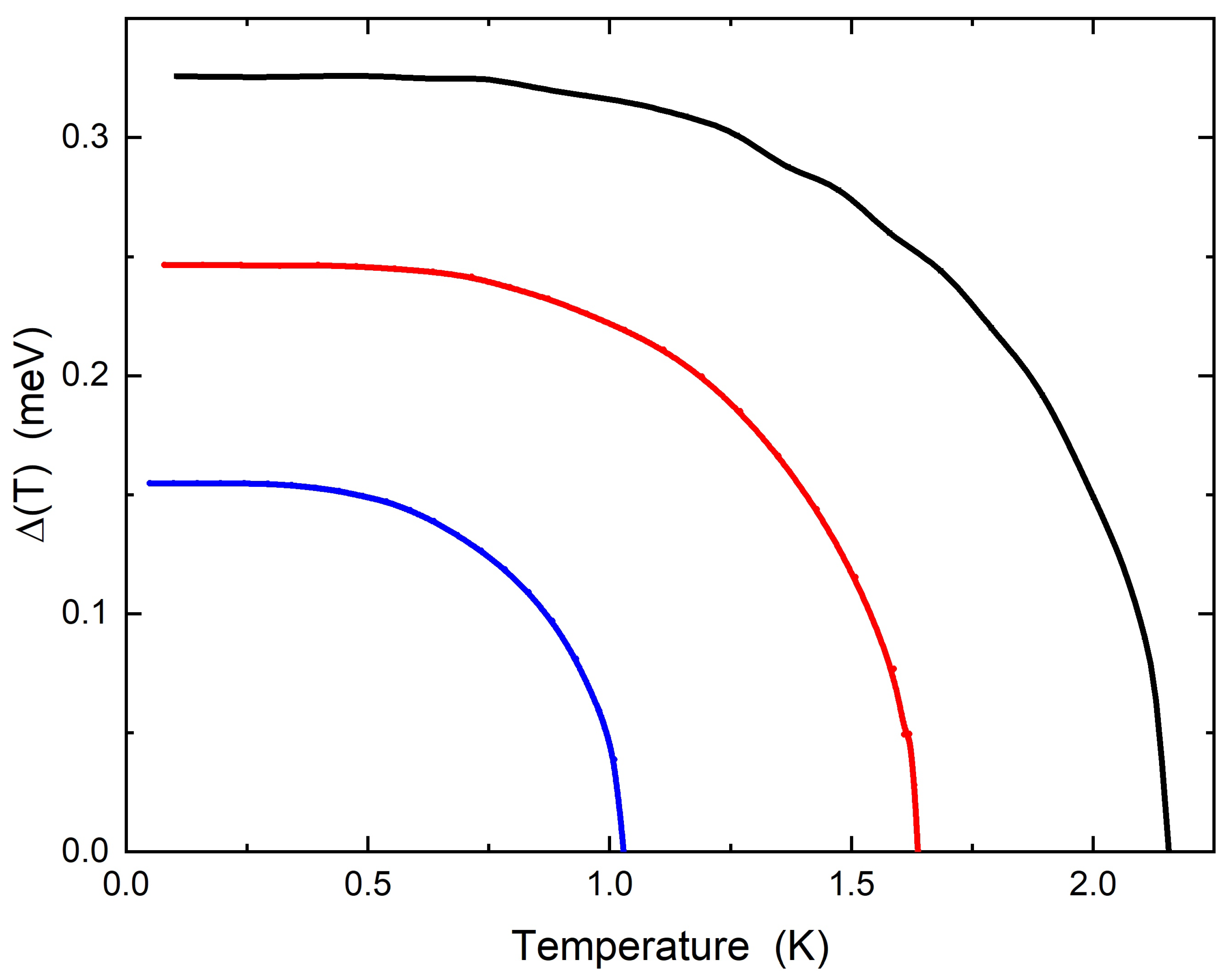
Figure 4.
Superconductive gap versus temperature for three different film thicknesses Å: the full solid lines in black, red and dark blue represent the numerical solutions of Eliashberg equations.
In Figure 1, two physical quantities of magnesium, the electron–phonon coupling constant and the Coulomb pseudopotential, used in the theoretical calculations, are plotted as functions of the film thickness L. The bulk electron–phonon spectral function of magnesium [21] with is shown in the inset of Figure 1. The cut-off energy is meV and is related to the bulk value of the Coulomb pseudopotential [22], while the maximum electronic energy is meV. The values of the bulk Fermi energy and carrier density are, respectively, meV and m−3 [23]. This produces a critical thickness Å. Figure 2 shows the other two physical quantities that are present in the theory: the thickness L. Figure 1 shows what we anticipated in the text of the paper, precisely that, around the critical thickness value, the coupling constant has a slight increase. Will this increase in the value of the electron–phonon coupling constant sufficiently to produce the superconducting state? To check this, we will solve the modified Eliashberg equations and calculate the critical temperature . The result is shown in Figure 3. We find that, for the film thickness Å, (very close to the critical value Å), the material becomes a superconductor with K. We notice that the thickness range that allows superconductivity to exist is quite narrow, which can be understood based on the underlying topological-type transition [2]. We can see that, as soon as we move away from the critical value of film thickness, the abruptly goes to very small values, which we are not able to calculate, as it is too time-consuming for the code to reach convergence. Finally, we should also point out that solid films that are as thin as nm are still effectively described by three-dimensional physics, as shown plenty of times in the literature on the basis of experiments, theory, and atomistic simulations, e.g., cfr. [2,24], albeit with substantial corrections due to confinements such as those implemented in our theory.
4. Conclusions
To include the crucial effect of quantum confinement, we have generalized the Eliashberg theory, where the thickness of the thin film appears, as well as the density of free carriers. In this way, we are able to compute the superconducting properties of magnesium thin films in a fully quantitative way and with no free parameters. Upon decreasing the film thickness, the Fermi surface shape changes, as well as the , and this fact leads to the increase in the number of electronic states at the Fermi level. This situation leads to an increase, significantly, in the electron–phonon coupling and hence a surprisingly low superconductivity but experimentally measurable temperatures. These theoretical predictions reveal the possibility that magnesium thin films with a thickness close to 0.4–0.5 nm become superconducting. These predictions are relevant from both a fundamental and an applied point of view.
Author Contributions
G.A.U. and A.Z. contributed equally to conceptualization, methodology, formal analysis, original draft preparation and writing. All authors have read and agreed to the published version of the manuscript.
Funding
A.Z. gratefully acknowledges funding from the European Union through Horizon Europe ERC Grant number: 101043968 Multimech, from US Army Research Office through contract nr. W911NF-22-2-0256, and from the Niedersächsische Akademie der Wissenschaften zu Göttingen in the frame of the Gauss Professorship program.
Data Availability Statement
No new data were created or analyzed in this study. Data sharing is not applicable to this article.
Acknowledgments
G.A.U. acknowledges partial support from the MEPhI.
Conflicts of Interest
The authors declare no conflict of interest.
References
- Ummarino, G.A.; Zaccone, A. Quantitative Eliashberg theory of the superconductivity of thin films. J. Phys. Condens. Matter 2025, 37, 065703. [Google Scholar] [CrossRef] [PubMed]
- Travaglino, R.; Zaccone, A. Extended analytical BCS theory of superconductivity in thin films. J. Appl. Phys. 2023, 133, 033901. [Google Scholar] [CrossRef]
- Ummarino, G.A.; Zaccone, A. Can the noble metals (Au, Ag, and Cu) be superconductors? Phys. Rev. Mater. 2024, 8, L101801. [Google Scholar] [CrossRef]
- Bianconi, A.; Missori, M. High Tc superconductivity by quantum confinement. J. Phys. I 1994, 4, 361. [Google Scholar]
- Ummarino, G.A. Emergent Phenomena in Correlated Matter; Pavarini, E., Koch, E., Schollwöck, U., Eds.; Forschungszentrum Jülich GmbH and Institute for Advanced Simulations: Jülich, Germany, 2013; pp. 13.1–13.36. [Google Scholar]
- Carbotte, J.P. Properties of boson-exchange superconductors. Rev. Mod. Phys. 1990, 62, 1027. [Google Scholar] [CrossRef]
- Varlamov, A.A.; Galperin, Y.M.; Sharapov, S.G.; Yerin, Y. Concise guide for electronic topological transitions. Low Temp. Phys. 2021, 47, 672. [Google Scholar] [CrossRef]
- Landrò, E.; Fomin, V.M.; Zaccone, A. Topological Bardeen–Cooper–Schrieffer theory of superconducting quantum rings. Eur. Phys. J. B 2025, 98, 7. [Google Scholar] [CrossRef]
- Inkof, G.A.; Schalm, K.; Schmalian, J. Quantum critical Eliashberg theory, the Sachdev-Ye-Kitaev superconductor and their holographic duals. NPJ Quantum Mater. 2022, 7, 56. [Google Scholar] [CrossRef]
- Larkin, A.; Varlamov, A.A. Theory of Fluctuations in Superconductors; OUP Oxford: Oxford, UK, 2005; Volume 127. [Google Scholar]
- Ummarino, G.A.; Gonnelli, R.S. Breakdown of Migdal’s theorem and intensity of electron-phonon coupling in high-Tc superconductors. Phys. Rev. B 1997, 56, R14279. [Google Scholar] [CrossRef]
- Ummarino, G.A.; Gonnelli, R.S.; Stepanov, V.A. Eliashberg equations with energy dependence of the normal density of states and quasiparticle tunneling in high-Tc superconductors. Nuovo Cimento D 1997, 19, 1215. [Google Scholar] [CrossRef]
- Ummarino, G.A.; Gonnelli, R.S. Possible explanation of electric-field-doped C60 phenomenology in the framework of Eliashberg theory. Phys. Rev. B 2002, 66, 104514. [Google Scholar] [CrossRef]
- Mitrovi´c, B.; Carbotte, J. Effects of energy dependence in the electronic density of states on some superconducting properties. Can. J. Phys. 1983, 61, 784. [Google Scholar] [CrossRef]
- Schachinger, E.; Carbotte, J.P. Thermodynamic properties of strong coupling superconductors with energy-dependent electronic density of states. J. Phys. F Met. Phys. 1983, 13, 2615. [Google Scholar] [CrossRef]
- Allen, P.B.; Dynes, R.C. Transition temperature of strong-coupled superconductors reanalyzed. Phys. Rev. B 1975, 12, 905. [Google Scholar] [CrossRef]
- Torsello, D.; Ummarino, G.A.; Gozzelino, L.; Tamegai, T.; Ghigo, G. Comprehensive Eliashberg analysis of microwave conductivity and penetration depth of K-, Co-, and P-substituted BaFe2As2. Phys. Rev. B 2019, 9, 134518. [Google Scholar] [CrossRef]
- Torsello, D.; Ummarino, G.A.; Bekaert, J.; Gozzelino, L.; Gerbaldo, R.; Tanatar, M.A.; Canfield, P.C.; Prozorov, R.; Ghigo, G. Tuning the Intrinsic Anisotropy with Disorder in the CaKFe4As4 Superconductor. Phys. Rev. Appl. 2020, 13, 064046. [Google Scholar] [CrossRef]
- Ghigo, G.; Ummarino, G.A.; Gozzelino, L.; Tamegai, T. Penetration depth of Ba1-xKxFe2As2 single crystals explained within a multiband Eliashberg s± approach. Phys. Rev. B 2017, 96, 014501. [Google Scholar] [CrossRef]
- Torsello, D.; Cho, K.; Joshi, K.R.; Ghimire, S.; Ummarino, G.A.; Nusran, N.M.; Tanatar, M.A.; Meier, W.R.; Xu, M.; Bud’ko, S.L.; et al. Analysis of the London penetration depth in Ni-doped CaKFe4As4. Phys. Rev. B 2019, 100, 094513. [Google Scholar] [CrossRef]
- Leonardo, A.; Sklyadneva, I.Y.; Silkin, V.M.; Echenique, P.M.; Chulkov, E.V. Ab initio calculation of the phonon-induced contribution to the electron-state linewidth on the Mg(0001) surface versus bulk Mg. Phys. Rev. B 2007, 76, 035404. [Google Scholar] [CrossRef]
- Burnell, D.M.; Wolf, E.L. Proximity-effect tunneling study of Mg. J. Low Temp. Phys. 1985, 58, 61. [Google Scholar] [CrossRef]
- Ashcroft, N.; Mermin, D. Solid State Physics; Cengage Learning, Inc.: Philadelphia, PA, USA, 2021. [Google Scholar]
- Yu, Y.; Yang, C.; Baggioli, M.; Phillips, A.E.; Zaccone, A.; Zhang, L.; Kajimoto, R.; Nakamura, M.; Yu, D.; Hong, L. The ω3 scaling of the vibrational density of states in quasi-2D nanoconfined solids. Nat. Commun. 2022, 13, 3649. [Google Scholar] [CrossRef] [PubMed]
Disclaimer/Publisher’s Note: The statements, opinions and data contained in all publications are solely those of the individual author(s) and contributor(s) and not of MDPI and/or the editor(s). MDPI and/or the editor(s) disclaim responsibility for any injury to people or property resulting from any ideas, methods, instructions or products referred to in the content. |
© 2025 by the authors. Licensee MDPI, Basel, Switzerland. This article is an open access article distributed under the terms and conditions of the Creative Commons Attribution (CC BY) license (https://creativecommons.org/licenses/by/4.0/).